
the Creative Commons Attribution 4.0 License.
the Creative Commons Attribution 4.0 License.
 | 07 Jul 2026
Characterising mesoscale magnetopause surface waves within magnetosphere–ionosphere–ground coupling

David Southwood
Song Zhang
Qiran Sun
Mike Heyns
Disturbances to the magnetopause location driven by upstream pressure variations or flow shear instabilities may be described as surface waves, which act as localised sources of field-aligned currents coupling the magnetosphere to the ionosphere. However, their impacts on the ionosphere and ground across representative ranges of wave and system properties are poorly understood. We, therefore, develop a simple numerical model for dispersionless mesoscale magnetopause surface waves within the coupled magnetosphere–ionosphere–ground system to gain insight into how their amplitudes and spatial scales throughout the system might vary with conditions. In general, the impacts of finite wave packets can be decomposed into periodic fluctuations (with matching wavelength to that directly above in the magnetosphere) along with slowly-varying trends that result from finite wave effects. Finite wave packets act in the far-field like a string of alternating field-aligned currents well described both in the ionosphere and on the ground as a two-dimensional current dipole. In the ionosphere, near-field periodic fluctuations exponentially decay over the reduced wavelength latitudinally away from the projected magnetopause boundary layer flux tubes, which may limit how well they can be resolved by radar. The relationship between the magnetic field above and below the ionosphere becomes more complicated for surface waves than infinite plane Alfvén waves due to the additional spatial structure, which introduces interference across the spectrum of wavenumbers present. This modifies how the ionosphere screens, rotates, and spatially smears magnetic field perturbations across all three components in different ways. For mesoscale wavelengths this importantly results in latitudinal scales of amplitude and polarisation variation smaller than typical ground magnetometer spacings, motivating the need for denser networks. A range of effective skin depths in the ground are applicable to surface waves, meaning ground induction can vary between a near-perfect insulator to a good conductor, affecting both observable ground magnetic fields and resulting geoelectric fields. The predicted peak amplitudes of surface waves' impacts suggest they may act as significant sources of ionospheric/thermospheric Joule heating and geoelectric fields in the ground, thereby contributing to space weather impacts. These are, however, highly localised latitudinally when considering typical mesoscale waves. Our results provide key insight into interpreting ground-based observations, of particular timeliness with the rollout of new digital ionospheric radars and the SMILE mission's planned conjugate ground–space campaigns.
- Article
(11814 KB) - Full-text XML
- BibTeX
- EndNote


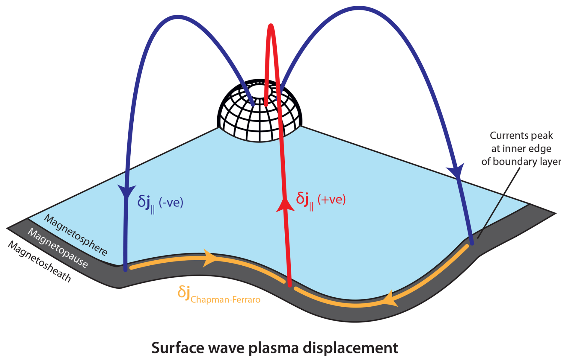
Field-aligned currents (FACs) are the main physical mechanism mediating magnetosphere–ionosphere (MI) coupling (e.g. Ganushkina et al., 2018), dynamically connecting/transferring energy to and from these geospace regions. Magnetospheric ultra-low frequency (ULF, ∼0.1–100 mHz) waves contribute to variability in this coupling and are often described using magnetohydrodynamics (MHD; Jacobs et al., 1964; Wright et al., 2024). In basic theory the only MHD body wave (free to propagate through the bulk plasma) to exhibit FACs is the shear Alfvén mode. However, discontinuities separating different plasmas allow surface waves (Archer et al., 2024b, and references therein), collective evanescent fast magnetosonic modes that support FACs within the plasmas' interface (Plaschke and Glassmeier, 2011). Magnetopause surface modes at the solar–terrestrial interaction's interface impose a wave pattern of plasma displacements on the boundary. When the wavelength and amplitude of these displacements is larger the boundary layer’s thickness, a single coupled surface mode across the entire boundary layer exists rather than distinct modes at the different interfaces (Kivelson and Pu, 1984). This surface wave compresses/rarefies the magnetic field on either side of the equatorial magnetopause in opposite senses and by different amounts, locally enhancing/diminishing the Chapman-Ferraro current. These perturbation currents within the closed field lines of the boundary layer are diverted, preserving current continuity, from largely perpendicular to magnetospheric field lines to along them, becoming FACs which then close in the ionosphere as longitudinally periodic currents. An illustration of this is shown in Fig. 1. Therefore, magnetopause surface waves directly influence the ionosphere and ground (Kivelson and Southwood, 1988; Archer et al., 2023), unlike other compressive waves which do so secondarily via coupling to Alfvén waves due to non-uniformities in the bulk plasma/magnetic field (Southwood and Kivelson, 1990, 1991).
Magnetopause surface waves play a global role in filtering, accumulating, and guiding turbulent solar wind driving (Kivelson and Chen, 1995; Archer et al., 2024b). They form on the boundary maintaining total pressure balance, excited either by upstream pressure variations (originating from the solar wind, foreshock, or magnetosheath; e.g. Sibeck et al., 1989; Shue et al., 2009) or grow from seed fluctuations due to velocity shear instabilities (Kelvin–Helmholtz instability, KHI; e.g. Fairfield et al., 2000). The surface wave dispersion relation dictates how the boundary responds to different driving regimes. While the general dispersion relation can only be solved numerically, if incompressibility is assumed it has analytic solution
for wave angular frequency ω, transverse wave vector kt, velocities u, mass densities ρ, and magnetic fields B, where subscript 0's indicate equilibria, “msp” is the magnetosphere, and “msh” the magnetosheath (Chandrasekhar, 1961; Pu and Kivelson, 1983). Given typical conditions at the magnetopause, a simpler approximate dispersion relation
holds when (Archer et al., 2024b). Equation (1) consists of a natural surface wave frequency for no flow shear due to standing field-aligned structure, ω0 (Chen and Hasegawa, 1974), along with an advective Doppler shift by the background magnetosheath flow. Along most of the magnetopause, frequencies are dictated by the magnetosheath velocity () and perpendicular wavelengths (), with negligible natural frequency () (Miura and Pritchett, 1982; Kozyreva et al., 2019). Typical equatorial wavelengths ∼2–14 RE (azimuthal wavenumbers m∼4–30 for exp (imϕ) dependence) and periods ∼1–7 min are observed (Lin et al., 2014). However, around the subsolar point the magnetosheath is slow (), hence the natural frequency dominates () leading to a resonant magnetopause surface eigenmode (MSE) response to (particularly impulsive) external driving (Archer et al., 2019). This constitutes the lowest-frequency eigenmode of the dayside magnetosphere, typically less than 2 mHz (Plaschke et al., 2009a; Archer and Plaschke, 2015; Hartinger et al., 2015b). While MSE from solar wind forcing are global in scale (Hartinger et al., 2015b; Archer et al., 2021), bow shock/magnetosheath transients of several RE in size (m∼20–60) also cause MSE (Archer et al., 2019). In the absence of continuous driving or instabilities, surface modes are strongly damped, likely resulting in only a few cycles at a time (Chen and Hasegawa, 1974; Kozyreva et al., 2019).
Magnetopause surface waves penetrate the magnetosphere over evanescent e-folding scale , the reduced/angular wavelength. Thus global and mesoscale waves significantly affect geospace and subsequently couple to other modes (Horvath and Lovell, 2021; Archer et al., 2021, 2022). This leads to mass, momentum, and energy transport into geospace, contributing to the viscous-like solar–terrestrial interaction in absence of global magnetic reconnection (Axford, 1964). Understanding magnetopause surface waves' energy pathways, particularly with regards to the ionosphere and ground, is therefore important, especially within the context of space weather. It is being appreciated more that ULF waves significantly contribute to ionospheric energy input (e.g. Hartinger et al., 2015a). This results in ionospheric/thermospheric dissipation via Joule heating (e.g. Shi et al., 2025a), and induced geoelectric fields (e.g. Hartinger et al., 2020; Shi et al., 2022, 2025b) that drive currents in power grids (e.g. Belakhovsky et al., 2019; Heyns et al., 2021).
Theoretically ULF waves' effects in the ionosphere and on the ground have focused on Alfvén waves. Seminal analytic results on the ionosphere's effects of rotating ground magnetic field fluctuations by 90° (Hughes, 1974; Hughes and Southwood, 1974) and screening small-scale (compared to the ionospheric altitude) waves (Hughes and Southwood, 1976) all rely on the assumption of plane Alfvén waves vertically incident on a homogeneous ionosphere. Given limitations with analytic theory, later works have simulated Alfvén wave transmission using the linearised wave equations in more representative setups, e.g. incorporating dipole magnetic geometries (Lysak, 2004), improved boundary conditions (Lysak and Song, 2006), asymmetric ionospheric conductances (Lysak et al., 2020), or including multiple altitude-varying ion and neutral species (Sydorenko and Rankin, 2012). Theoretical models of the MI-response to upstream pressure variations have not directly invoked surface modes on the magnetopause, instead considering fast–Alfvén coupling Earthward of the boundary (Sibeck, 1990; Southwood and Kivelson, 1990, 1991). The direct effects of magnetopause surface waves have only recently been appraised through high-resolution general-purpose global MHD simulations (Archer et al., 2023). This pertained to impulsively-excited large-scale azimuthally-stationary MSE across the dayside, which seeded tailward propagating surface waves in the flanks (Archer et al., 2021). Surface wave FACs at the MI-interface peaked at the equatorward edge of the magnetopause boundary layer (MPBL), as depicted in Fig. 1, rather than the open-closed boundary (OCB). Earthward of the MPBL, weaker FACs decaying with distance occurred via fast–Alfvén coupling which exhibited slow poleward phase motion due to damping. The result in the ionosphere was convection vortices circulating FAC structures. The ground magnetic field response was predominantly, but not entirely, controlled by Hall currents. This is because Fukushima's (1976) theorem of the perfect cancellation of field-aligned and Pedersen current effects below the ionosphere only holds for semi-infinite FACs along straight vertical field lines (for either a planar or spherical ground geometry) and uniform ionospheric Pedersen conductance. The ground magnetic field was rotated from the magnetosphere by close to 90° on average, but with significant angular spread interpreted as due to violation of Fukushima's (1976) theorem. While these basic features are expected for any process generating FACS, e.g. Alfvénic field line resonances (Greenwald and Walker, 1980), and have long been associated with magnetospheric dynamics in observations (e.g. Friis-Christensen et al., 1988; Glassmeier and Heppner, 1992; Glassmeier, 1992; Bristow et al., 1995), it is the FACs' structure and the scales of variations which might enable discrimination between different dynamical phenomena. The effect of induction in the ground and thus whether surface waves specifically lead to significant geoelectric fields remains an open question (Archer et al., 2023).
Evidence for magnetopause surface modes from ground-based instruments alone was inconclusive for a long time (Pilipenko et al., 2017, 2018; Kozyreva et al., 2019), largely due to a lack of robust theoretical expectations and the scarcity of ground–space conjunctions during clear surface wave events (Archer et al., 2019). The Archer et al. (2023) simulation results demonstrated qualitative agreement with previous candidate ground-based events (Archer et al., 2019; Kozyreva et al., 2019; He et al., 2020; Hwang et al., 2022). Key aspects could not be tested with the data presented though, motivating both reanalysis of these events and dedicated future observational studies. While global MHD models self-consistently reproduce magnetopause surface waves within a representative environment, quantitative predictions from any single run strictly apply to the specific driver, set of upstream conditions, and geospace plasma configuration used, caveated by the numerics' effects on results (e.g. Zhang et al., 2019; Archer et al., 2024b). More widely-applicable comparisons between theory and observations require a comprehensive characterisation of expected surface wave responses in the ionosphere and on the ground across broad representative ranges of both wave and system conditions. However, many of these are not easily tuneable in such simulations. Additionally, the resolution required to resolve the wave physics throughout geospace make these simulations computationally expensive, hence impractical for parameter searches, rendering results more generally qualitative. Dedicated linear ULF wave simulations with dipole or more generalised geometries also exist which are more configurable (Degeling et al., 2010; Wright and Elsden, 2020; Lysak et al., 2020). Magnetopause surface waves have yet to be simulated in a realistic manner within these codes (Elsden et al., 2025), since such waves serve as the imposed outer boundary condition requiring a priori knowledge of the solution. Given the basic physical insight analytic MHD applied to highly simplified environments have provided (e.g. Southwood, 1974; Chen and Hasegawa, 1974; Hughes and Southwood, 1974), we opt to develop a simple local model to advance understanding of how magnetopause surface waves' effects within magnetosphere–ionosphere–ground (MIG) coupling might scale spatially and in amplitude across key wave and system parameters. We introduce the model and its numerical implementation in Sect. 2, derive some analytic relations in Sect. 3, and then compare these with numerical results in Sect. 4.
2.1 Model
Using simple “toy” models initially in physics can provide physical insight and intuitive understanding to a problem, as well as enabling computational efficiency, serving as foundational tools for framing hypotheses, testing limiting cases, and bridging the gap to complex simulations. While not realistic by design, their complexity can be iterated through a step-by-step reduction of assumptions once the physical effects that are important are better understood from the simple model results. Thus “toy” models serve as an essential first step in addressing a new science question.
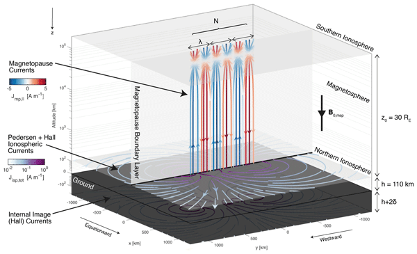
There are few geometries in which linear MHD surface waves can be derived analytically (Archer et al., 2024b); even those with orthogonal curvilinear coordinates (such as a dipole or cylinder) can only be solved when invoking several assumptions and still yield complicated expressions (Nenovski et al., 2007; Leonovich and Kozlov, 2019). Therefore, we opt to use one of the simplest geometries, the Cartesian box model that has long been leveraged for initial physical insights into ULF waves (e.g. Southwood, 1974) and is often still applied to surface wave problems (Plaschke and Glassmeier, 2011; Archer et al., 2023; Elsden et al., 2025). Employing the electric field and current paradigm, common of the ionosphere (Vasyliunas, 2001; Laundal et al., 2015), we solve a boundary value problem using current continuity through different conducting layers to determine the spatial structure of solutions through the coupled MIG-system given imposed magnetopause currents due to a mesoscale surface wave. In order to make our results more general and independent of any specific background, we only incorporate current systems due to the surface wave in this model, hence all responses presented are solely due to waves. The classical Region 0/1/2 FAC systems and their ionospheric counterparts serve as a time-constant (though spatially varying) background to the linear equations solved, which do not affect the wave response and can easily be separated out. Our setup is illustrated in Fig. 2a, along with the various physical quantities the model outputs applied to a single example (panels b–r).
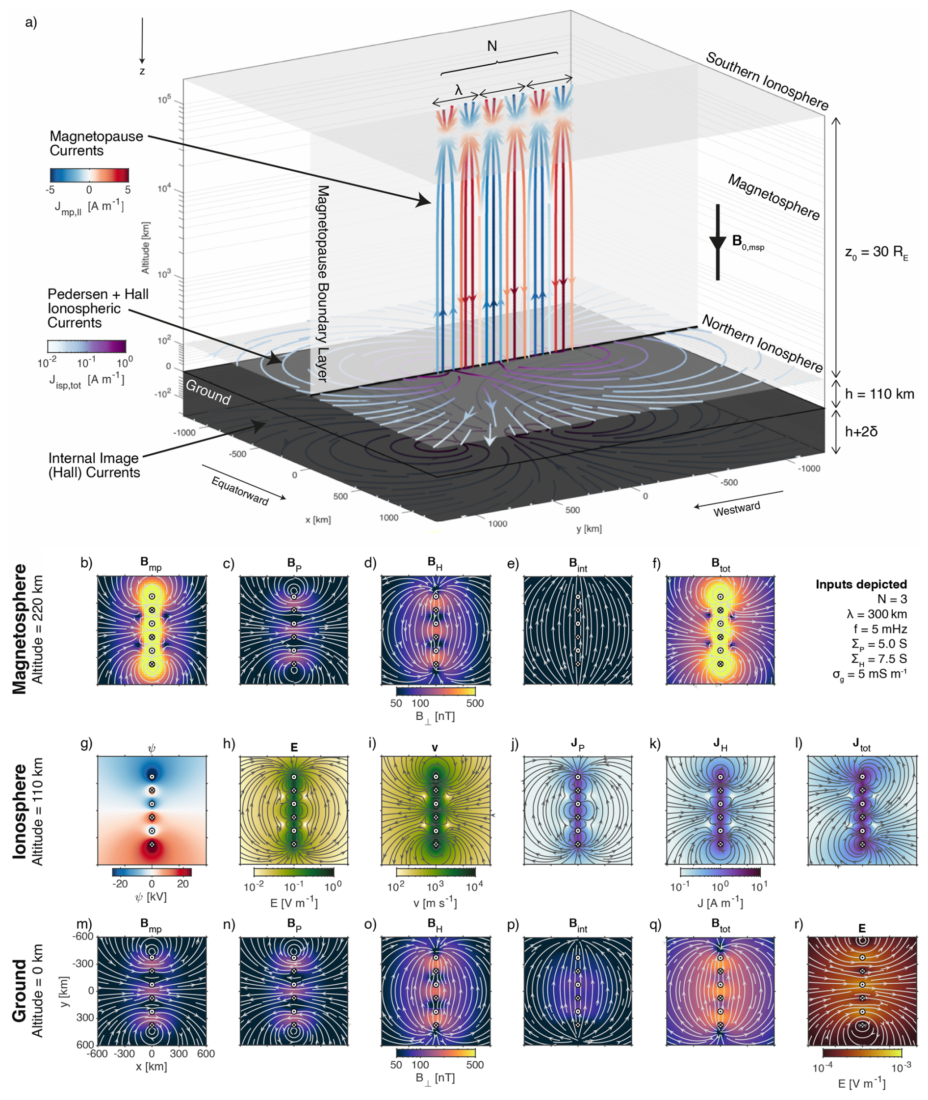
Figure 2(a) Diagram of the surface wave magnetosphere–ionosphere coupling model showing the current systems for a finite magnetopause surface wave packet: (field-aligned) magnetopause currents, ionospheric Pedersen and Hall currents, and internal currents via the complex image method. Example model outputs are shown in the low-altitude magnetosphere (b–f), ionosphere (g–l), and on the ground (m–r). Shown are the ionospheric potential (g), electric field (h), drift velocity (i), and Pedersen (j), Hall (k), and total (l) currents; along with the horizontal magnetic field (f, q) and contributions to this from magnetopause (b, m), Pedersen (c, n), Hall (d, o), and internal (e, p) currents; and finally the horizontal geoelectric field (r). Only the imaginary parts are depicted.
At equilibrium the model consists of two uniform half-spaces, the magnetosheath and magnetosphere, separated by the magnetopause around x=0. In the magnetosphere (x>0) the geomagnetic field is uniform with vertical field lines of length z0, appropriate for high-latitudes. The full field line is included for self-consistency within the model, but little affects results. This geometry is translationally invariant. Thin-shell ionospheres in the northern and southern hemispheres are located at and , respectively. The northern hemisphere ground corresponds to z=0, where points equatorward, is westward, and is down (such coordinates are common for ULF waves, Southwood, 1974; geophysical induction, Thomson and Weaver, 1975; and ground magnetometers, Landal and Gjerloev, 2014). Therefore, in the ionosphere x<0 corresponds to open field lines in the polar cap. This is appropriate since there is little evidence that the magnetosphere is ever entirely closed under even prolonged northward interplanetary magnetic field, with in practice some regions of open flux still remaining (Raeder, 1999; Vennerstrom et al., 2005; Bhattarai and Lopez, 2013). Since scales of uniform box models cannot be globally representative and our focus is on ground-observable effects due to principally ionospheric current systems, it is at the MI-interface where the box model must be most representative of physical scales and conditions. Thus horizontal scales up to 1250 km from the origin are considered, corresponding to the distance to the horizon from ionospheric altitude. This necessarily makes our model local to the field lines which map to the mesoscale magnetopause surface wave, hence we make no comment on the global state of the magnetosphere.
Plaschke and Glassmeier (2011) derived the electrical currents for an infinite wave train of incompressible MHD magnetopause surface waves within a box model by finding solutions on closed field lines and requiring continuity of pressure and normal velocity across the (assumed infinitesimally-thin) boundary. The surface waves in this model exhibit standing structure along closed field lines between conjugate points in the ionosphere, established via ionospheric wave reflection (Kivelson and Southwood, 1988). Their expressions for the amplitudes of the surface currents must also hold for the total current within a finite-width boundary via the integral form of Ampère's law. Archer et al. (2023) demonstrated surface wave currents peak on the closed field lines at the inner/equatorward edge of the magnetopause boundary layer (MPBL), yielding longitudinally periodic FACs at the MI-interface (see Fig. 1). The equatorial magnetopause current sheet is typically ∼500 km thick (Berchem and Russell, 1982), which projected along Tsyganenko (1995) model field lines corresponds to ionospheric width d∼40 km (8 % the magnetospheric value). This is much smaller than projected surface mode wavelengths ∼250–3000 km. Therefore, for simplicity, we can represent magnetopause currents as having infinitesimal-thickness at x=0, strictly corresponding to the closed field lines at the inner/equatorward edge of the projected MPBL flux tubes. This approach does not affect ionospheric currents outside the MPBL due to Gauss's law.
Here ξ0 is the amplitude of boundary displacements in the equatorial magnetosphere and we have neglected the influence of the magnetosheath magnetic field on the currents since (Plaschke and Glassmeier, 2011). The resulting current amplitude into/out of the ionosphere is surprisingly independent of azimuthal wavelength for all realistic ionospheric scales ().
Since surface modes are highly-damped, we model finite trains of constant-amplitude purely-sinusoidal waves. This is achieved by multiplying the (complex phasor) currents in Eq. (3) by a rectangular function of total width Nλ centred on y=0, where N is the number of cycles, giving zero net FAC at the MI-interface. This simple rectangular modulation is unlike the typical picture of a wave packet, which usually has a smooth envelope. The finite wave packet constitutes a localised mesoscale source of FACs, as depicted in Fig. 2a. The rectangular function introduces a sinc spectrum of wavenumbers about ky, which in general might lead to dispersion. However, the approximate surface wave dispersion relation (Eq. 1) has two dispersionless limits. The first corresponds to propagating waves where the frequency is controlled by the magnetosheath flow , typically valid in the flanks (ω0 negligible; Chandrasekhar, 1961; Miura and Pritchett, 1982; Kozyreva et al., 2019), with phase and group velocities . The second are azimuthally stationary waves at fixed frequency ω≃ω0, typical of the subsolar magnetopause (u0,msh negligible; Chen and Hasegawa, 1974; Archer et al., 2021, 2023), which has zero group velocity. Stationary waves are formed from a superposition of waves with opposite azimuthal wavenumbers, equivalent to taking the imaginary part spatially while keeping the complex time variation. This makes our model static, since magnetopause currents form time-invariant structures that either propagate downtail or are stationary. Our focus is determining the spatial structure of the waves transmitted through the system. Note, the rectangular function introduces discontinuities at the wave packet edges in FACs' real parts, hence the imaginary parts (displayed throughout Fig. 2) are more representative of potential measurements.
Electrostatic MI-coupling is applied to the northern hemisphere ionosphere (e.g. Wolf, 1975), solving the ionospheric (isp) potential ψ through current continuity ()
where Σ denotes the height-integrated conductivity tensor (or conductance) consisting of Pedersen (P) and Hall (H) conductances, both assumed uniform. Current continuity is appropriate in the absence of ionospheric induction when (Yoshikawa, 2002; Lotko, 2004; Lysak and Song, 2006), found to be across the ranges explored. Given the ionospheric potential (example shown in Fig. 2g), the ionospheric electric field E, plasma drift velocity v, and currents are obtained
with examples displayed in Fig. 2h–l. By symmetry, signatures in the southern hemisphere should be mirror reflections of those in the northern hemisphere.
Often in modelling work the ground is treated as either a perfect insulator (e.g. Tanaka et al., 2020), where no telluric/internal currents are induced in the ground (particularly in global MHD simulations), or a perfect conductor (e.g. Hughes, 1974; Hughes and Southwood, 1974), where there is no geoelectric field and telluric currents lead to no vertical ground magnetic field while doubling the horizontal components from MI-currents. Clearly neither regime is realistic. The Complex Image Method (CIM) provides a simplification to the general induction problem (Weaver, 1971) for oscillatory MI-currents by placing image currents at a depth for complex skin depth δ (Wait and Spies, 1969; Thomson and Weaver, 1975; Boteler and Pirjola, 1998). While this approximation is technically valid for skin depths much smaller/larger than either the characteristic horizontal scale (Thomson and Weaver, 1975) or distance to the source (Wait and Spies, 1969), Pirjola and Viljanen (1998) report in practice CIM works very well across all typical parameter ranges in geomagnetic induction (much wider than considered here). They also detail how to apply CIM to arbitrary horizontal and vertical current systems. Given constant ionospheric conductance this is equivalent to image currents equal and opposite to the ionospheric Hall currents here, as shown in Fig. 2a. For simplicity we consider uniform ground conductivity σg, resulting in skin depth
Given our model does not rely on all parameters in the surface wave dispersion relation (Eqs. 1–2) we are free to set the frequency independently.
Magnetic fields can be evaluated at any location using the Biot–Savart law, the general solution to Ampère's law when retarded time can be ignored (Griffiths and Heald, 1991),
and are computed for the magnetopause, Pedersen, Hall, and internal current systems separately along with their totals, as shown in Fig. 2 on the ground (panels m–q) and above the ionosphere (panels b–f). Finally, the horizontal geoelectric field Eg is found via the Coulomb gauge magnetic vector potential A
Pirjola's (1998) procedure in our model is equivalent to applying these only to the ionospheric and image Hall currents. Unlike for the ground magnetic field, contributions from each current system have no physical meaning thus only the total is calculated, as shown in Fig. 2r. Since the skin depth is complex, calculations differ for propagating and stationary waves (the currents' imaginary part must first be taken for stationary waves).
The limitations of this deliberately simple model and how results from it may be modified through more sophisticated modelling in the future is discussed in Sect. 5.2.
2.2 Numerical implementation
Given the large number of parameters that can be varied within this model, we choose to investigate effects of the ionospheric wavelength, Pedersen and Hall conductances, ground conductivity, and the number of wave oscillations on the surface wave response throughout the system. Ionospheric conductances control the amount of current carried through the ionosphere, making them crucial to MIG-coupling. Representative values between 1.5–12 S are used (Ridley et al., 2004). Wavelengths also strongly affect Alfvén wave transmission to the ground (e.g. Hughes and Southwood, 1976). Only horizontal scales up to 1250 km from the origin are physical within our model, corresponding to when the line-of-sight vector between a ground point and an ionospheric current source, as applicable in e.g. the Biot–Savart law, is tangent to the Earth's surface (similar reasoning applied to the curvature of field lines suggest scales comparable to the radius of curvature or L-shell, both of which are significantly larger than this at the high-latitudes applicable to the magnetopause). To mitigate edge effects magnetopause/ionosphere grids extend to ±2500 km. Given this domain size, we only consider ionospheric wavelengths between 200–1600 km, corresponding to m∼8–70 or ∼1–9 RE at the equatorial magnetopause ( factor from the ionosphere), covering the majority of the observed range. Since finite wave effects are also of interest given damping, we also vary the number of oscillations from one up to the maximum possible within our domain for each wavelength. Finally, a wide range of ground conductivities applicable from city (0.1 mS m−1) to salt water (5 S m−1) environments are considered, given the variety of ground magnetometer locations.
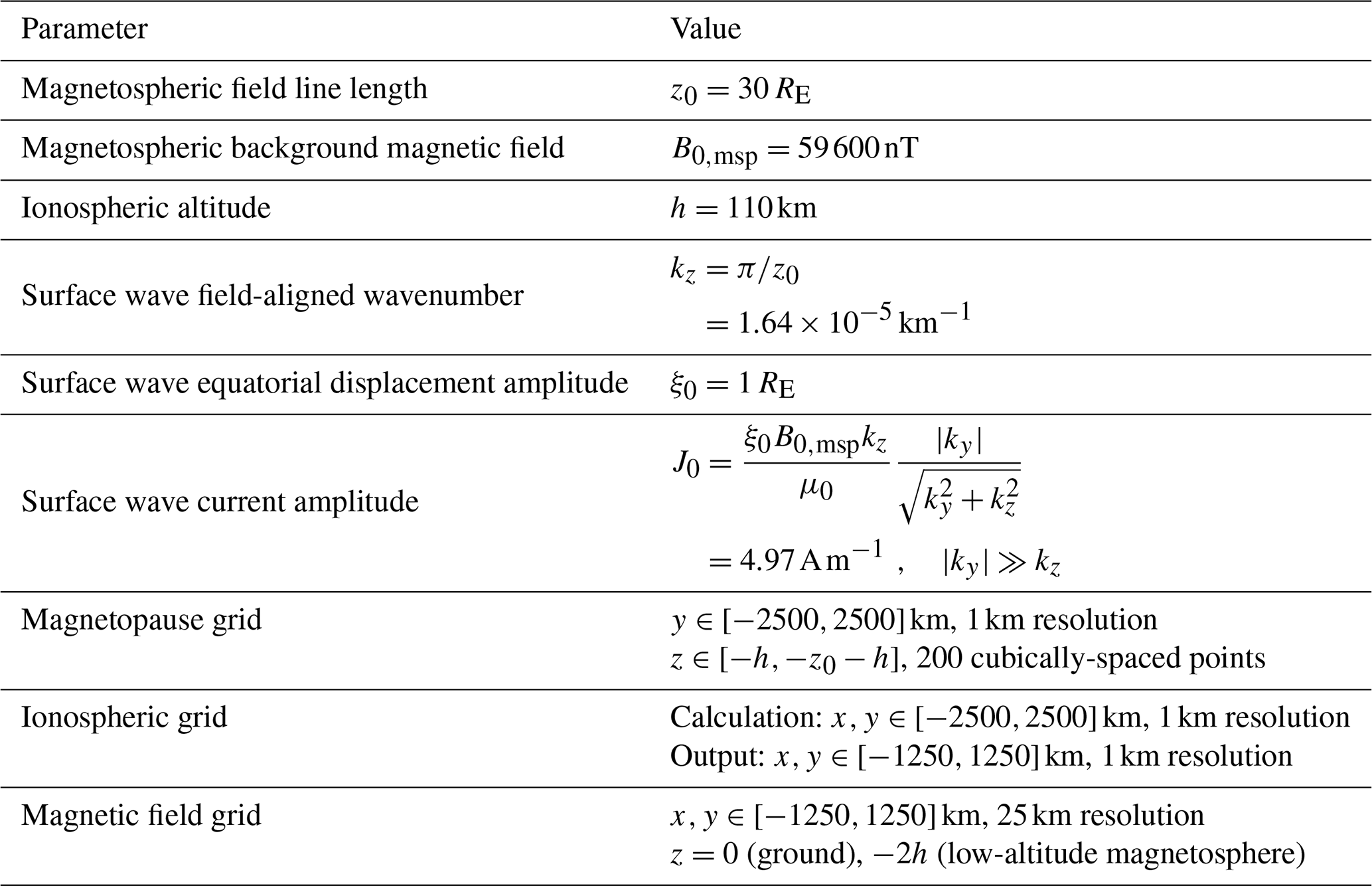
All other parameters are fixed as detailed in Table 1. The field line length is representative of the dayside magnetopause (e.g. Archer et al., 2022). The magnetospheric magnetic field is that of Earth's dipole at ionospheric altitude, with 70° magnetic latitude chosen for reference (e.g. Smith and Sojka, 2019). Given the E–j paradigm, it is crucial currents (the only physical quantity coupling different regions here) at the MI-interface are correct, dictating the choice of field strength. Note, these currents are unchanged when typical equatorial magnetospheric field and scales are instead used with dipole flux tube scaling subsequently applied (Goodman, 1995), since this rescales the current by the magnetic field ratio with J0 proportional to the local field and independent of ky. This further justifies the use of the magnetic field at the MI-interface here. We consider a fundamental magnetopause surface wave with 1 RE equatorial displacement, of similar magnitude to observed waves (e.g. Archer et al., 2019), which does not require rescaling to the ionosphere since its influence on the currents is accounted for by the magnetic field ratio discussed earlier. Changes to any of these fixed parameters simply rescale the wave's current amplitude J0 proportionally, hence it is easy to adjust results presented for different scenarios. The ionospheric altitude is set at the typically used E region value of 110 km.
Table 1Fixed parameters of the surface wave model and values used.
The ionospheric potential is solved using the Green's function (G) for the 2D Laplacian L
where denotes the perpendicular radius in cylindrical coordinates, such that
Integration is performed numerically using the trapezium rule, since this converges faster than Simpson's rule for periodic functions (Rahman and Schmeisser, 1990; Weideman, 2002). The ionospheric electric field is calculated with a second-order centred difference. Given the discontinuity at x=0, potentials at the midpoints between the discontinuity and adjacent gridpoints are calculated for improved gradients. The Biot–Savart law is also evaluated using the trapezium rule. These calculations are the most sensitive to grid resolution, hence we performed grid convergence tests on the ground magnetic field. We repeated calculations for 200 km wavelength (the shortest considered) in the range and fit a power law to the differences from the highest resolution (Δx=0.5 km). The average fractional error in the magnitude varied as and the angular error as , from which we chose 1 km resolution. While the same resolution was used for the magnetopause currents in y, the large scales along the magnetospheric magnetic field render a uniform grid inefficient. Given the integrand falls off at its fastest, we employ a cubically-spaced grid. Similar tests on the number of points along the field Nz showed errors converged quickly, with fractional error in magnitude of and angular error , leading us to settle on Nz=200.
Before presenting numerical results we first attempt to derive analytic relations to the surface wave effects in the ionosphere and ground, which is performed for two limiting cases. The first is the near-field, which should be well approximated by the simpler case of an infinite wave. This is particularly relevant for long wave trains, e.g. resulting from KHI (e.g. Fairfield et al., 2000) or solar wind periodic density structures (e.g. Viall et al., 2009). The second case is the far-field, pertinent to localised sources of FACs which result from a limited number of cycles, e.g. due to damping (Chen and Hasegawa, 1974; Kozyreva et al., 2019).
3.1 Ionosphere
3.1.1 Near-field approximation
For an infinite wave, Eq. (5) for the ionospheric potential becomes
By separation of variables we have
This is the Green's function problem for the “screened Poisson” or “modified Helmholtz” operator which leads to solutions (Abramowitz and Stegun, 2000; McLean, 2000; Schulz, 2001)
from which it is straightforward to derive the ionospheric electric field, drift velocity, and Pedersen and Hall currents
3.1.2 Far-field approximation
A finite FAC distribution centred on the origin with zero net current into/out of the ionosphere is a localised source of ionospheric dynamics. We can employ a multipole expansion of the electrostatic potential far from the extent of the current sources () to understand the large-scale impact of this localised source
where the current dipole moment p (analogous to the electric dipole moment in electrostatics) is
The concept of a current dipole is more readily used in biophysics (e.g. Cohen and Hosaka, 1976; Sarvas, 1987) and geophysics (Poikonen et al., 1997; GeoSci.xyz Project, 2015), describing a localised current source within a conducting medium. Indeed, our finite wave packet can be thought of as a string of current dipole sources (see Fig. 2a), hence the scaling with N. This leads to ionospheric potential in polar coordinates
from which the ionospheric electric field, drift velocity, and currents are derived (Eqs. 6–9)
Note these solutions are static in the frame of the wave packet travelling at for propagating waves, hence are not oscillatory.
3.2 Ground magnetic field
The Biot–Savart law (Eq. 11) applied to ionospheric currents for an infinite wave involves complicated integrals over sources in both x′ and y′ (Eqs. 14–15). While it is possible to evaluate the y′ integral, recovering that the ground magnetic field is periodic in y with wavenumber ky as expected, this leaves integrals of the form
where K is the modified Bessel functions of the second kind and different orders/exponents (α,β) apply to each component. We are not aware of any closed form for these integrals, hence cannot provide analytic solutions for the ground magnetic field in the near-field limit.
In contrast, the far-field approximation can be derived by considering an ideal current dipole – a pair of opposite semi-infinite FAC sources separated by distance d along the y axis. If we assume Fukushima's (1976) theorem is approximately valid, given that in our model field lines are vertical and ionospheric conductances are uniform, then one needs only consider the contributions from Hall currents. Using Eq. (13), Pirjola and Viljanen (1998) gave solutions to the magnetic vector potential due to Pedersen currents from a single FAC I at the origin
Since in our model , the vector potential due to Hall currents is
with ground (z=0) magnetic field
Considering sources at and series expanding about d=0 yields
Summing over both sources, converting back to cylindrical coordinates, and remembering the current dipole moment py=Id here, we then have
The limit R≫h is valid for typical magnetopause wavelengths when considering the far-field.
The Biot–Savart law applied to internal (image) currents takes the same form as for MI-currents, thus it is not possible to solve analytically in the near-field limit. In the far-field limit, disturbances due to a propagating wave packet are not periodic, instead varying slowly compared to ULF timescales leading to negligible telluric currents. On the other hand, stationary waves' disturbances will be periodic and one could use a similar approach to that above to derive approximate expressions. Given the more limited scope and that fields in this limit are likely small, we shall not consider them further.
3.3 Geoelectric field
As with the ground magnetic field, near-field solutions to the geoelectric field have no closed form we are aware of. Far-field solutions are again only appropriate for stationary waves, which for similar reasons we shall not assess here.
3.4 Outlook
It is clear that, even for the simplest model setup under several approximations, analytic solutions of surface wave transmission throughout the MIG-system are highly limited. The near-field for even an infinite wave has no closed form on the ground. While far-field solutions for finite FAC sources can be derived throughout the system, finite wave effects in the near-field (where they are most important) cannot be expressed in terms of elementary functions. This motivates numerical results within our model, guided by analytic theory, to elucidate scaling relations for surface wave transmission across the input parameters of interest.
We now present numerical results from our model, comparing these to theory from Sect. 3 where possible.
4.1 Ionosphere
The ionospheric impacts show distinct behaviours in the near- and far-field limits, as seen in Fig. 2g–l (imaginary parts are shown). Near the wave packet centre the potential (panel g) is similarly periodic in y (East–West) to the FACs, peaking at their maxima/minima (white circles), and decaying with distance perpendicular to the MPBL-projection, consistent with Sect. 3.1.1. These result in periodic ionospheric electric fields, velocities, and currents that all exibit maximum magnitudes along the MPBL. Pedersen currents (panel j) emanating from FAC sources close at their adjacent opposite polarity sinks, but are not simply confined to the East–West direction spreading out laterally also. An identical pattern occurs in the electric field (panel h) since the conductance is uniform. Hall currents form vortices around FAC maxima/minima (panel k), which are clockwise for downwards FACs and anticlockwise for upwards. Ionospheric flow vortices (panel i) with identical patterns but the opposite rotation sense are a result of the uniform conductances and magnetic field. All these features are qualitatively consistent with MHD simulations (Archer et al., 2023). Far-field ionospheric signatures are instead strongly influenced by the potentials near the ends of the wave train, which exhibit larger maxima/minima than in the centre. These result in electric fields and Pedersen currents that resemble a dipole field, as predicted in Sect. 3.1.2, and two large-scale vortices in both the flow and Hall currents. While this was not clear in the simulation of Archer et al. (2023), likely due to the larger wavelengths making spherical effects important, flow patterns at mid-latitudes certainly exhibited scales larger than the distance between adjacent opposite-polarity FACs.
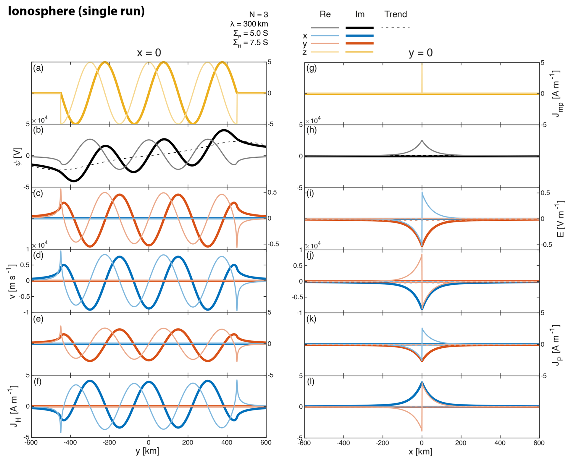
Figure 3Example ionospheric cuts along x=0 (a–f) and y=0 (g–l) of the field-aligned current (a, g), potential (b, h), electric field (c, i), drift velocity (d, j) and Pedersen (e, k) and Hall (f, l) currents. Both imaginary (thick, darker) and real (thin, lighter) parts of the solutions are shown. Background trends are shown as dashed lines where the Spearman rank correlation >0.5.
Figure 3 shows cuts along and perpendicular to the MPBL for the same model run, depicting both real (thinner/lighter) and imaginary (thicker/darker) parts. It is clear the surface wave's sinusoidal FACs at the MI-interface (panel a) result in similarly sinusoidal ionospheric properties within the extent of the wave train (panels b–f). However, fluctuations are not about zero as slight offsets and/or trends occur throughout the surface wave, most clearly seen in the potential (panel b) where the real part has a positive offset and the imaginary part exhibits a slope. Mathematically these arise from the Green's function integration resulting in a modulated complex phasor superposed with the logarithm of a polynomial. We apply a spline-based filtering method detailed in appendix A to extract the offsets/trends, shown by the dashed lines. Periodic fluctuations are then defined as the difference between the two, which we denote with tilde marks. These offsets/trends occur within the surface wave due to its finite extent. For an infinite wave an equally infinite number of FAC oscillations about zero exist to the left and right of any point along the MPBL, which leads to overall cancellation in the Green's function integration. In contrast, for a finite wave imbalances occur due to the applied rectangular function leading to unequal net currents to the left and right of points along the MPBL. While the discontinuity in the FACs' real part from the rectangular function leads to spikes in the real parts of all ionospheric quantities except the potential, only the imaginary parts are treated as physical. Along the MPBL, all signatures slowly reduce in magnitude with distance outside the wave packet. In contrast, perpendicular to the MPBL (panels h–l), ionospheric quantities appear to quickly exponentially decay with distance (as expected from near-field theory) with perturbations becoming negligible well within a single wavelength's distance. This means even relatively large-scale surface waves have highly localised impacts latitudinally. The model suggests ionospheric velocities up to several km s−1 and Joule heating rates up to hundreds of mW m−2 might result from large-amplitude magnetopause surface wave activity, those these peak values will be spatially concentrated. Ionospheric flows of tens of km s−1 have been reported in global simulations due to large-scale magnetopause motion (Slinker et al., 1999).
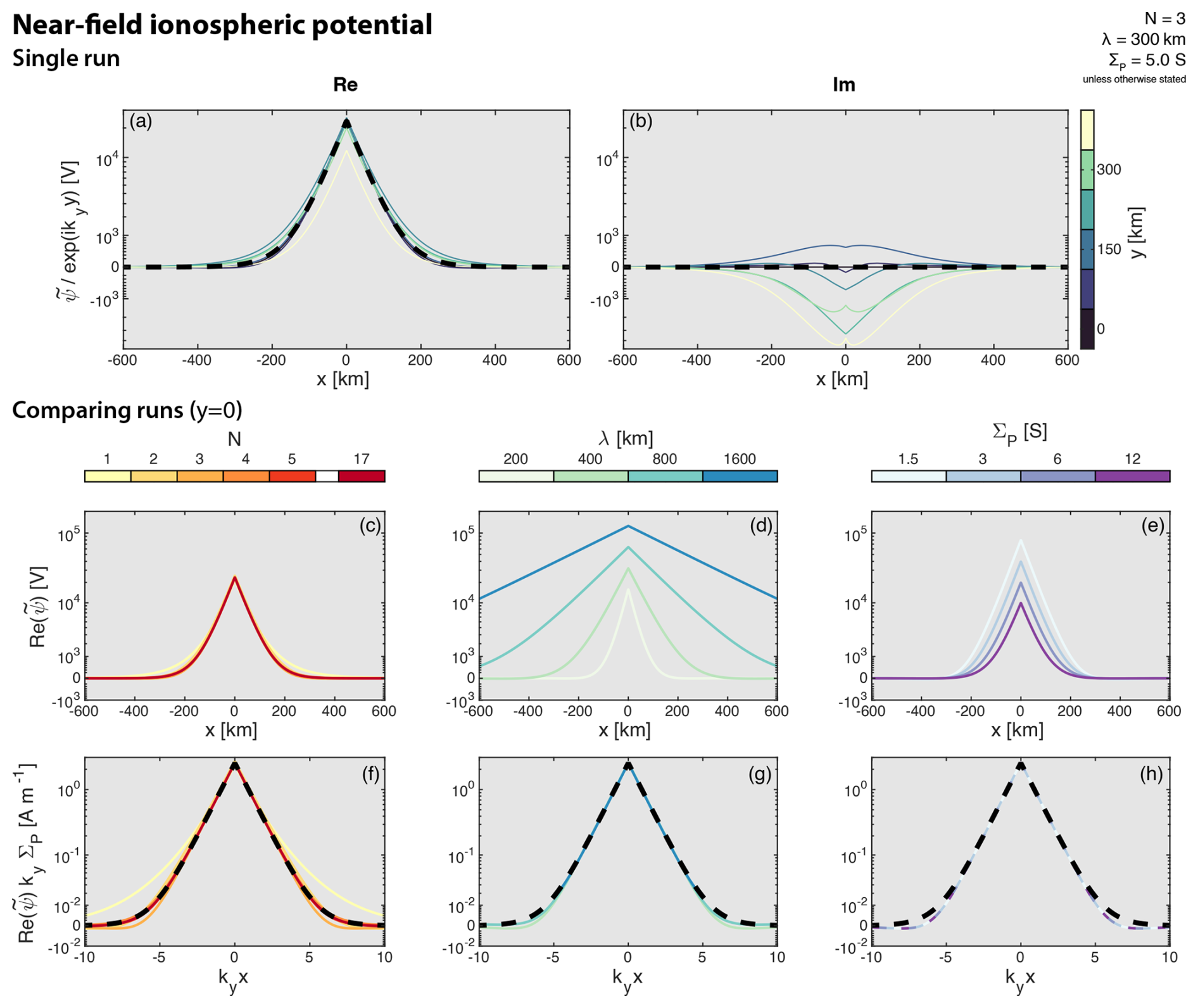
Figure 4Comparison of the ionospheric potential with near-field theory. (a, b) Example comparison across a single run. The fluctuating part of the potential is divided by a complex phasor, with real (a) and imaginary (b) parts shown as a function of x for various y-values (colours). (c–h) Comparison across runs varying model input parameters. The real part of the fluctuating potential along y=0 is shown (c–e) along with a normalised version of this (f–h) according to theory, such that curves should collapse on to one another and the theoretical solution (black dashed lines).
We now quantitatively compare ionospheric surface wave signatures to theory. Figure 4 examines the potential in the near-field limit. For a single set of model inputs, we extract the fluctuations in the potential and divide these by the expected complex phasor variation, with panels (a) and (b) depicting the real and imaginary parts, respectively, of the result as a function of x at different points along the y axis. This shows excellent agreement with the theoretical exponentially-decaying solution, given by the black dashed lines. Note, the e-folding scales for mesoscale waves (∼30–250 km) will not be well-resolved by typical ionospheric grid resolutions in global simulations (; Rastätter et al., 2014). For the dominant real part, the amplitude at the MPBL only significantly differs from theory when within a quarter-wavelength of the wave packet edge, where the infinite wave assumption breaks down. There is also a slight increase in discrepancies with distance from the MPBL. Close to the MPBL the potential will be dominated by the local FAC oscillations, whereas further away the influence from other adjacent oscillations will proportionally increase leading to differences between finite and infinite waves. Differences in the imaginary part tend to peak at/near the MPBL and grow with distance from the wave packet centre. We now also investigate how the potential changes when varying the model inputs. Panels (c)–(e) show the real part of the fluctuating potential along y=0, whereas panels (f)–(h) normalise this based on theory such that curves should collapse on to one another and the theoretical solution (black dashed). First we vary the number oscillations (panels c and f) from one up to the maximum possible within our model domain for this wavelength (later denoted Nmax), keeping all other inputs fixed. The number of oscillations does not significantly affect the amplitude or shape of the potential, with differences between all solutions and the theoretical curve only apparent when N is two or less. Increasing the wavelength (panels d and g) results in the fluctuating potential having increased amplitude and larger lateral extent, though these remain very localised with Half Width at Half Maximum (HWHM) values ranging between only ∼20–175 km for the wavelength range considered. The normalisation, which rescales both distances and amplitudes by ky, leads to excellent agreement between the different runs and the theoretical solution, with only slight differences as kyx becomes large. Finally, the Pedersen conductance (panels e and h) affects only the amplitude of the fluctuating potential with normalisation giving agreement between runs to within machine accuracy, as the constant conductance is simply a factor. Overall, the ionospheric signatures of a finite magnetopause surface wave are well approximated by the infinite wave solutions for small .
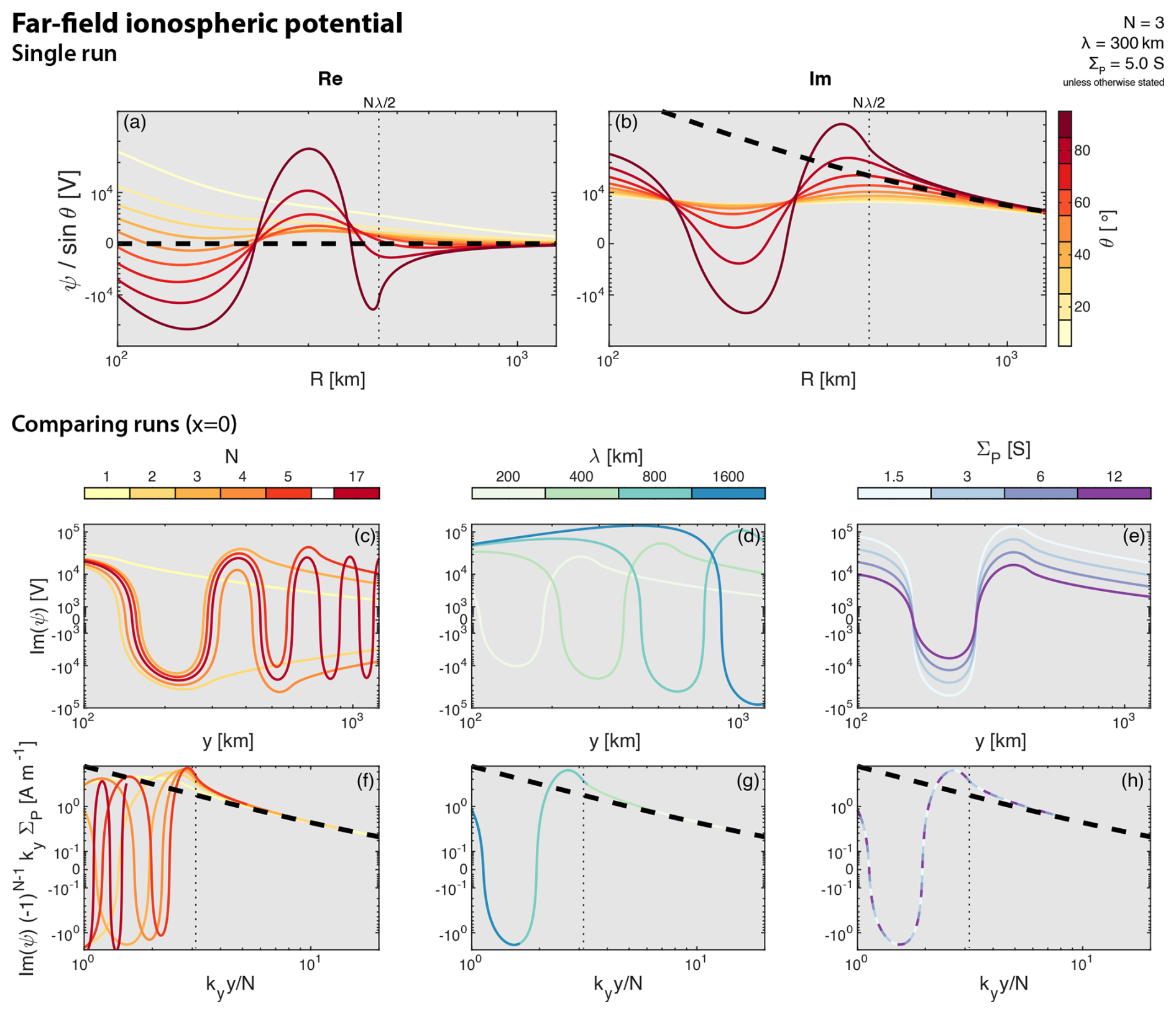
Figure 5Comparison of the ionospheric potential with near-field theory in a similar format to Fig. 4. (a, b) Example comparison across a single run. The real (a) and imaginary (b) parts of the potential are divided by sin θ and shown as a function of perpendicular radial distance for various azimuths. (c–h) Comparison across runs varying model input parameters. The imaginary part of the potential along x=0 is shown (c–e) along with its theory-normalisation version (f–h). Theoretical solutions (blacked dashed lines) are also shown. Vertical dotted lines indicate the radial extent of the current distribution.
For the far-field, we initially compare the ionospheric potential to theory for a single set of model inputs. Figure 5a–b show the real and imaginary parts, respectively, of the potential divided by sin θ as a function of perpendicular radial distance for a range of polar angles. While the red curves are along the periodic surface wave FACs, resulting in undulating potentials within the finite wave packet's extent (denoted by the vertical dotted line), the yellow curves are perpendicular to the MPBL hence do not exhibit this feature. For distances greater than the wave packet size, applicable to the far-field, the potential's real part tends towards zero and the imaginary part asymptotes to the theoretical dependence given by the black dashed line. The numerical solutions appear to converge faster as the polar angle approaches 90°, i.e. along the MPBL. As before, we then vary model inputs individually, comparing the potential's imaginary part along the MPBL. The sign of the far-field potential (panel c) changes with N, with odd N yielding positive values and even N giving negative ones. The normalisation used here rescales distances according to N, such that the wave train sizes become identical, given by the vertical dotted line in panels (f)–(h). This results in the different model solutions tending towards one another and far-field theory outside of the wave packet. It is clear that, similar to the near-field case, increasing the wavelength (panel d) leads to both larger scales and amplitudes. Accounting for these in the normalisation (panel g) leads to excellent agreement between the different potentials, which again asymptote towards theory. Finally, the Pedersen conductance (panels e and h) again serves as a simple dividing factor. We thus conclude that far-field theory agrees well with our numerical solutions for large .
4.2 Ground
Model outputs for the ground, as shown in Fig. 2m–r, are the contributions to the ground magnetic field from magnetospheric, ionospheric, and internal currents, as well as the geoelectric field.
4.2.1 Magnetic field (MI-currents)
We first consider the ground magnetic field only due to magnetospheric and ionospheric currents. The horizontal field patterns associated with the magnetopause and Pedersen currents appear similar but opposite to one another, meaning the ground field is dominated by Hall currents. Such cancellation is only perfect when field lines are vertical, ionospheric conductances are uniform, and FACs are of semi-infinite extent (Fukushima, 1976), whereas only the first two criteria strictly hold here. As with the ionosphere there are distinct near- and far-field patterns. The far-field, which resembles two vortices for the magnetopause and Pedersen current systems and a dipole for the Hall currents, dominate the ground magnetic field compared to near-field perturbations, which are difficult to discern in the streamlines but cause clear modulation of the horizontal field strength. This is likely the ionosphere screening the smaller scales (Hughes and Southwood, 1976). Further evidence of this can be seen comparing the magnetic field computed at the same distance above the ionosphere (panels b–f), which exhibit overall larger field strengths principally due to magnetopause currents (ionospheric currents yield equal but opposite contributions to those on the ground). Finally, ground field orientation appears close to a systematic 90° rotation from that above the ionosphere due to magnetospheric currents. While expected for an infinite plane Alfvén wave when the background field is vertical and conductances are uniform (Hughes, 1974; Hughes and Southwood, 1974), Archer et al. (2023) showed this does not exactly hold for a surface wave. Indeed, closer inspection of the rotation angle yields a bimodal distribution with distinct closely located peaks at 85° and 95° and overall standard deviation 14° for this example. At distinct wave phases along the MPBL-projection the sense of the rotation even becomes reversed, i.e. −90°, returning to normal within half a wavelength perpendicular to the MPBL. This further demonstrates the rule-of-thumb becomes altered for even simple changes to wave structure, such as with a finite surface wave.
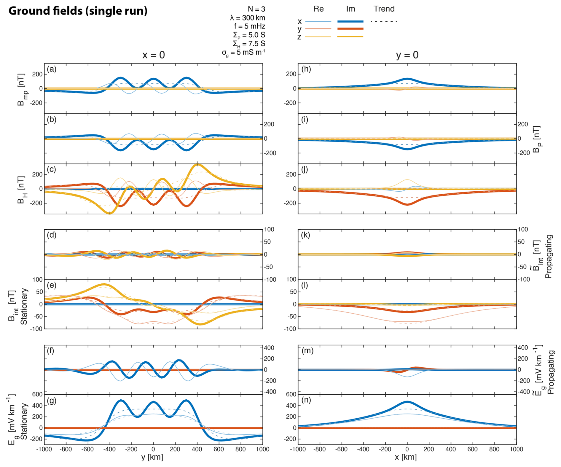
Figure 6Example ground cuts along y=0 (a–e) and x=0 (h–l) in a similar format to Fig. 3. Contributions to the ground magnetic field from magnetopause (a, h), Pedersen (b, i), Hall (c, j) and internal (d–e, k–l) currents, and the geoelectric field (f–g, m–n) are shown. Where required these are shown separately for propagating and stationary surface waves.
Figure 6 shows cuts along (panels a–c) and perpendicular to (h–j) the projected MPBL. Similar to with the ionosphere, the ground magnetic field shows sinusoidal behaviour along y about background trends/offsets (estimated by the dashed lines). These trends/offsets appear more significant than in the ionosphere, e.g. the fluctuation amplitude only constitutes half the total field perturbation near the MPBL. Perpendicular to the MPBL the magnetic field is smoothly varying, unlike the sharp exponential decay in the ionosphere, and the characteristic decay scale appears larger too. All these effects are likely a result of Biot–Savart spatial integration smearing wave effects out further and/or ionospheric screening of smaller-scale features. However, despite the smearing/screening, perturbation amplitudes are still significant at several hundreds of nT, in agreement with observed candidate events (e.g. Kozyreva et al., 2019). The figure also demonstrates that the fields due to magnetopause (a and h) and Pedersen (b and i) currents cancel to within 1 nT accuracy. Fukushima's (1976) theorem is thus an excellent approximation in our model. While not strictly valid, since the surface wave's magnetopause currents are not semi-infinite FACs, the scale of variation along the field in the magnetosphere are much longer than those across the field (ky≫kz), likely making it a reasonable approximation. In contrast, Archer et al. (2023) found greater discrepancies in a box model when using several RE perpendicular wavelengths, representative of magnetospheric scales. Given, however, that the ground field rotation by the ionosphere still significantly differed from 90° means this cannot result from the violation of Fukushima's (1976) theorem, but may instead be due to the non-planar wave structure (Hughes, 1974; Hughes and Southwood, 1974). In global MHD simulations of large-scale magnetopause surface waves, while the ground magnetic field is principally due to Hall currents, only a complex superposition of all current systems fully describes the total variance (Archer et al., 2023).
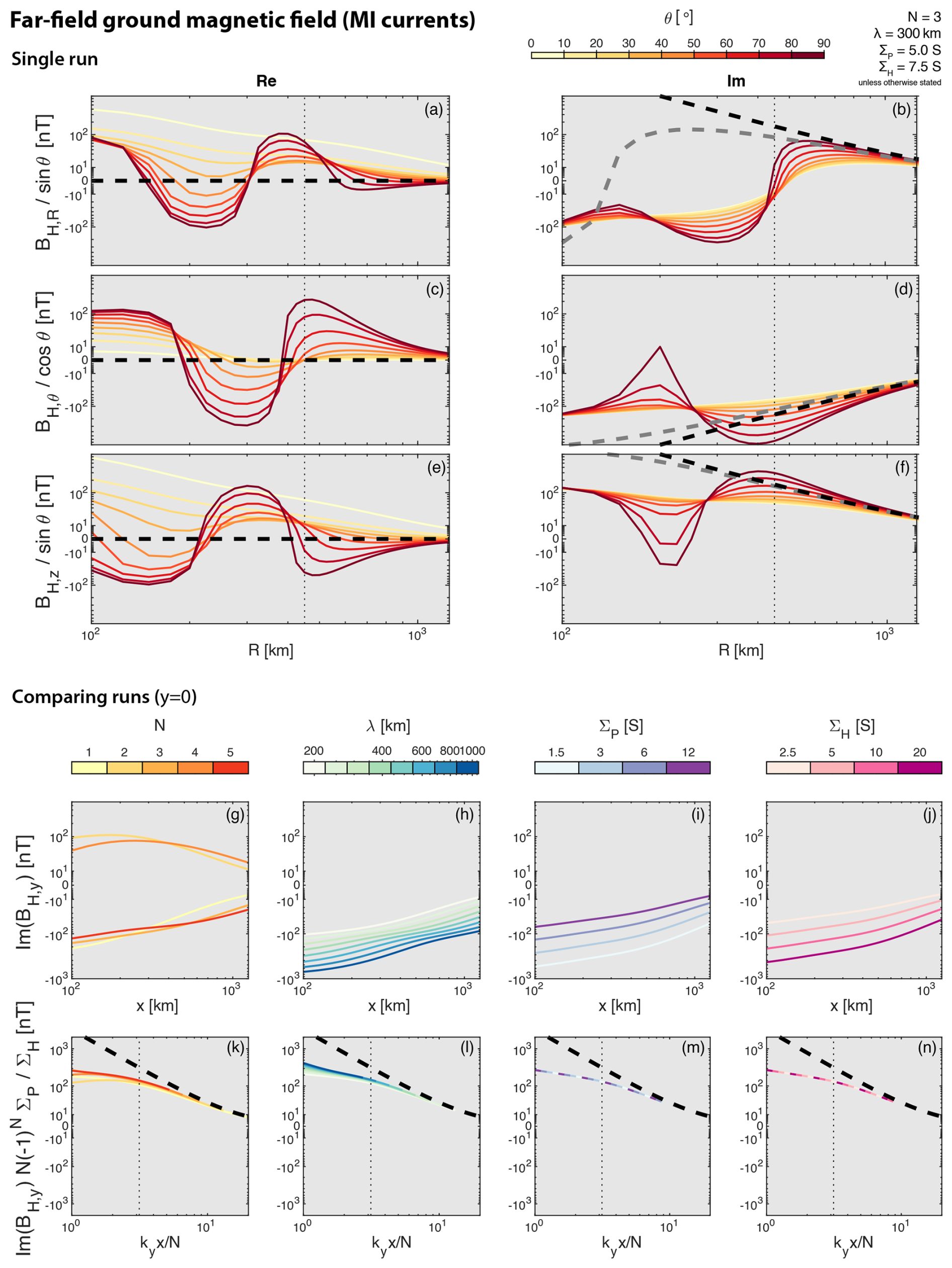
Figure 7Comparison of the ground magnetic field with far-field theory in a similar format to Fig. 5. (a–f) Example comparison across a single run in cylindrical coordinates. Shown as a function of perpendicular radial distance are the real (a, c, e) and imaginary (b, d, f) parts of the radial (a, b), azimuthal (c, d), and vertical (e, f) components divided by trigonometric functions based on theory for various azimuths (colours). (g, h) Comparison across runs varying model input parameters. The imaginary parts of the field are shown along y=0. Inputs varied (indicated by colour) are the number of oscillations (g, k), wavelength (h, l), and Pedersen (i, m) and Hall conductances (j, n). Theoretical solutions are shown (dashed lines) in their full form (grey) and the R≫h asymptotic limit (black).
We compare the numerical results with far-field theory (Sect. 3.2) in Fig. 7. Firstly we compare results in cylindrical coordinates from a single model run across a range of polar angles. Plotted as a function of perpendicular radius are the three components of the ground magnetic field due to Hall currents, with panels (a), (c), (e) depicting the real part and (b), (d), (f) the imaginary. For distances greater than the wave's extent, the field tends towards zero in the real and a dependence in the imaginary. This is in good agreement with theory for R≫h (black dashed), necessarily the case here as there is little difference when this assumption is relaxed (grey dashed). As was found in the ionosphere, the ground magnetic field converges on the theoretical curves most quickly along the y axis. We then study how model inputs affect the far-field ground magnetic perturbations, again varying each input individually across panels (h)–(j) and normalising results based on theory in panels (k)–(n). Throughout the imaginary part of the y component along the x axis is shown. Like with the ionospheric potential, the direction of the magnetic field alternates between odd and even N (panel g). We again normalise the distance by N, such that wave packets' extents are identical and depicted by the vertical dotted line in panel (k)–(n). Theory dictates that, unlike with the ionosphere, this should leave a residual dependence on the ground magnetic field. Panel (k) accounts for this and shows the curves for all runs do tend towards theory (black dashed). Ground magnetic perturbations increase in amplitude with wavelength (panel h) and are well-accounted for by normalising distances (panel l), again giving good agreement with theory. Finally reducing the Pedersen (panel i) and/or increasing the Hall (panel j) conductances lead to increased ground fields, with these being simply reciprocal and multiplicative factors (panels m–n) as expected. Thus our numerical results are shown to be in excellent agreement with far-field theory.
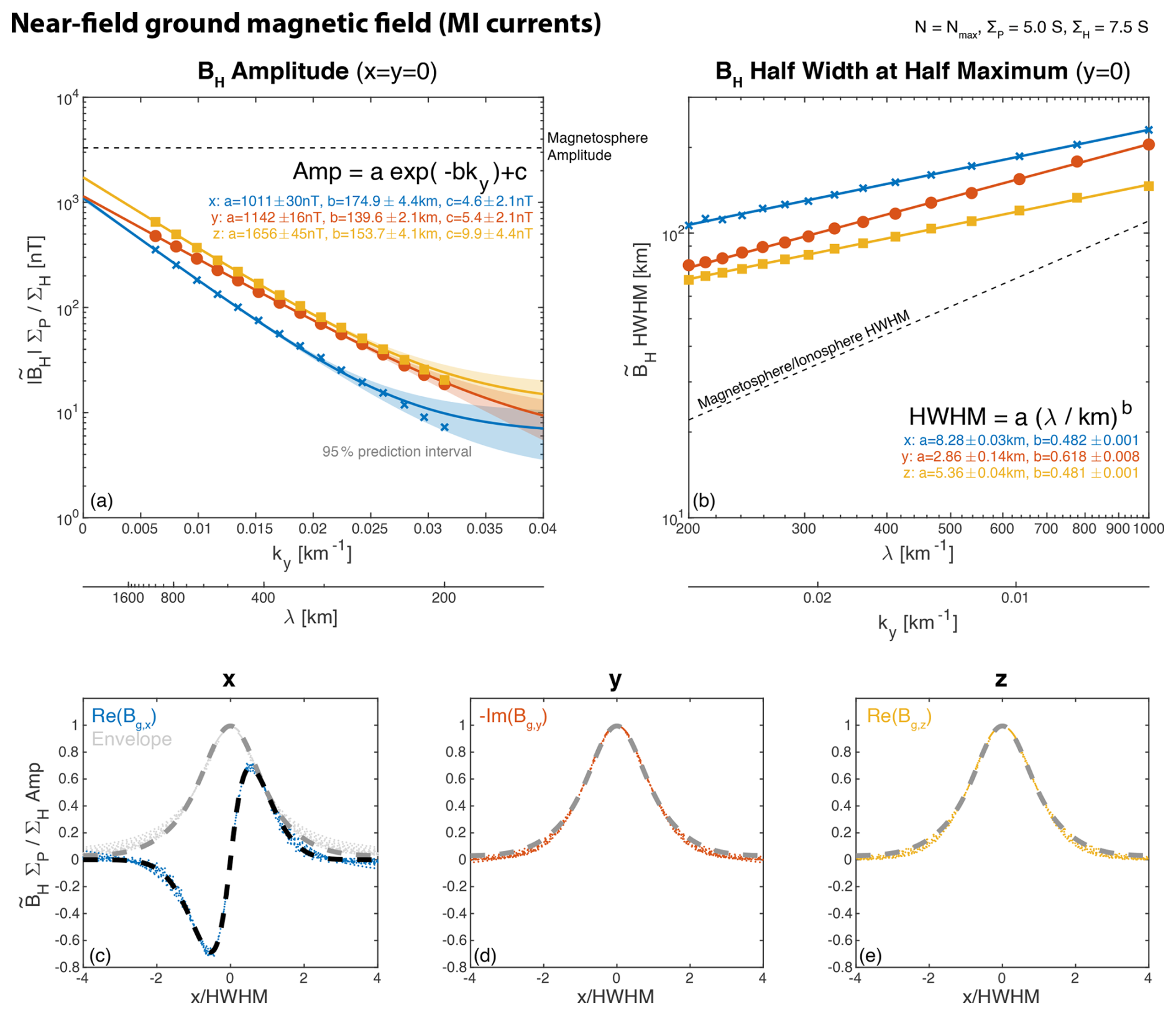
Figure 8Characterising the external ground magnetic field for pseudoinfinite waves. (a) Amplitude at x=0 of the x (blue crosses), y (red circles), and z (yellow squares) components as a function of wavenumber. (b) Half width at half maximum along the x axis for the three components as a function of wavelength. In both panels solid lines indicate fits to the data with shaded areas showing their 95 % prediction intervals. Bottom panels show the data along the x axis for all wavenumbers/wavelengths and normalised by both amplitude and half width at half maximum for the x (c), y (d), and z (e) components as coloured dots. For the x component the analytic envelope from a Hilbert transform is also shown (grey). Illustrative bell-shaped functional fits to the data are depicted by dashed lines.
We now move to the near-field, where no analytic form could be determined, modelling pseudoinfinite waves by setting the number of cycles to the maximum possible in the domain Nmax for each run. Throughout Fig. 8 the effect of the wavelength on the (Hall) ground magnetic field fluctuations is investigated. Panel (a) shows through markers the amplitudes of all three components at the origin multiplied by the conductance ratio. For the x component, which follows an odd function passing through zero at x=0 (Fig. 6j), we use the analytic signal envelope via a Hilbert transform in x to extract a suitable amplitude (see Fig. 8c). Across all wavelengths considered, amplitudes are lower than those in the magnetosphere (given by Plaschke and Glassmeier, 2011, and depicted as the horizontal dashed line), even when considering typical conductances (Ridley et al., 2004). All three components appear to follow an exponential decay law with ky, akin to the relation of Hughes and Southwood (1976) for infinite plane Alfvén waves where the e-folding scale is the ionospheric altitude. We, therefore, fit a decaying exponential to the data for each component using nonlinear least squares with robust iterative bisquare weighting (Huber, 1981). To account for systematic errors in the numerical modelling, a constant term is included in the fit. The results are shown as the solid lines along with their 95 % prediction intervals (shaded areas) and fit coefficients are listed in the figure. These reveal ground field amplitudes of up to a few thousand nT may be possible in the limit of large-scale waves. Note, while ky=0 results in no FACs hence no ionospheric or ground signatures, the FAC amplitude quickly becomes within 5 % of J0 for ky≈3kz, only slightly altering the upper limit of ground amplitudes. Signals are strongest in the vertical component for all wavelengths (∼20–40 % larger than ). This component is generally associated with FACs if ground inductive effects can be neglected – Eq. (16) demonstrates the magnetic field due to Hall currents resulting from an isolated FAC are significantly stronger in the vertical, exhibiting a prominant peak directly below the FAC. Therefore, given a surface wave constitutes a string of alternating FACs, it is not surprising that the vertical field component is strongest. Interestingly, the e-folding scale with ky is larger than the ionospheric altitude and varies for each component, ranging between ∼140–180 km. The Hughes and Southwood (1976) relation was derived requiring electric and magnetic fields in the atmosphere, ionosphere, and magnetosphere follow the same plane wave ansatz, clearly not the case for a surface wave. In theory one can decompose any problem into its consituent wavenumbers and still apply their result. Based on this, a larger decay scale would be expected, given that surface waves necessarily exhibit a spectrum of total wavenumbers . However, our numerical work highlights that the interference pattern between the different wavenumbers, even for this relatively simple example, can yield unexpected results. Heuristically, the magnitude of these decay scales can be rationalised through the Fourier transform of the ionospheric solutions
Calculating an average kx for this distribution as the Fourier-weighted root-mean-square gives corresponding to ∼176 km total e-folding scale from the magnitude of the full wave vector, broadly consistent with the numerical results. The surface wave has three distinct directions (along the magnetospheric field, and both along and perpendicular to the MPBL), whereas an infinite plane wave has only two (along either the field and the perpendicular wave vector component) and a single FAC only has one (the field direction). This means different behaviours might be expected for a surface wave in all three components. Indeed, this has already been seen in the ionosphere with sign changes across the MPBL in only one component of the two-dimensional currents. Therefore, it is perhaps not surprising that the three ground field components behave differently. An unexpected consequence though is the polarisation of waves as observed on the ground must become altered by the ionosphere from the circular polarisation in the magnetosphere (Plaschke and Glassmeier, 2011). Ground observed ULF waves are often assumed to provide remote sensing of the same waves originating in the magnetosphere, with the only ionospheric considerations being a 90° rotation and screening of smaller-scale waves (e.g. Ozeke et al., 2009). We have shown the introduction of even simple structure beyond a plane wave can dramatically change the one-to-one association from above to below the ionosphere.
For the same runs we also determine the Half Width at Half Maximum (HWHM) along the x-direction of the ground field perturbations, with results shown in Fig. 8b (for the x component this is again applied to the analytic signal envelope). While in both the magnetosphere and ionosphere a linear relation between HWHM and wavelength exists, as depicted by the dotted line, we find that not only are the scales larger on the ground but they appear to follow power laws. Given the form of the latitudinal Biot–Savart integral, this scaling is likely due to the Bessel function multiplication theorem (Abramowitz and Stegun, 2000)
a form of power law scale invariance preserving the fundamental spectral behaviour. Such behaviour is perhaps not surprising given dispersionless waves are scale invariant and power laws often result in self-similar natural models. We again apply fits, revealing the power law exponents are all less than unity and significantly differ between the three components. The latitudinal HWHM, the largest of the three components, while still greater than those in the magnetosphere and ionosphere range only ∼100–200 km even for reasonably large-scale waves up to ∼1000 km wavelengths (equivalent to m∼14 at 70° magnetic latitude). The vertical component has the smallest scales of ∼70–150 km. The different exponents for the two horizontal components means they approach one another for large wavelengths. Different latitudinal scales of amplitude variation across components of the ground magnetic field were also found in a global MHD simulation of large-scale surface waves (Archer et al., 2023), again with the vertical being smallest. Note, these resulting latitudinal scales comparable to the ionospheric altitude are not in violation of Hughes and Southwood (1976), since the longitudinal wavelengths considered are greater than h and only the total wavenumber applies in ionospheric screening. Our results are a consequence of the interference between the different attenuated wavenumbers in x. Interestingly, these latitudinal HWHM are smaller than the typical ∼200–300 km closest separations of ground magnetometer chains (Archer et al., 2024a) and typical global MHD ground-based output grids (Brenner et al., 2025), meaning such networks/simulations might not well resolve mesoscale surface waves. The different power laws for each component result in further polarisation changes on the ground compared to space.
For all the runs depicted in Fig. 8 we normalise the magnetic field profiles according to their amplitude and HWHM, shown as the dots in panels (c)–(e), which collapses them onto one another. More suprisingly, this normalisation renders all three components following the same profile (though in the case of the x component this applies to the analytic signal envelope).
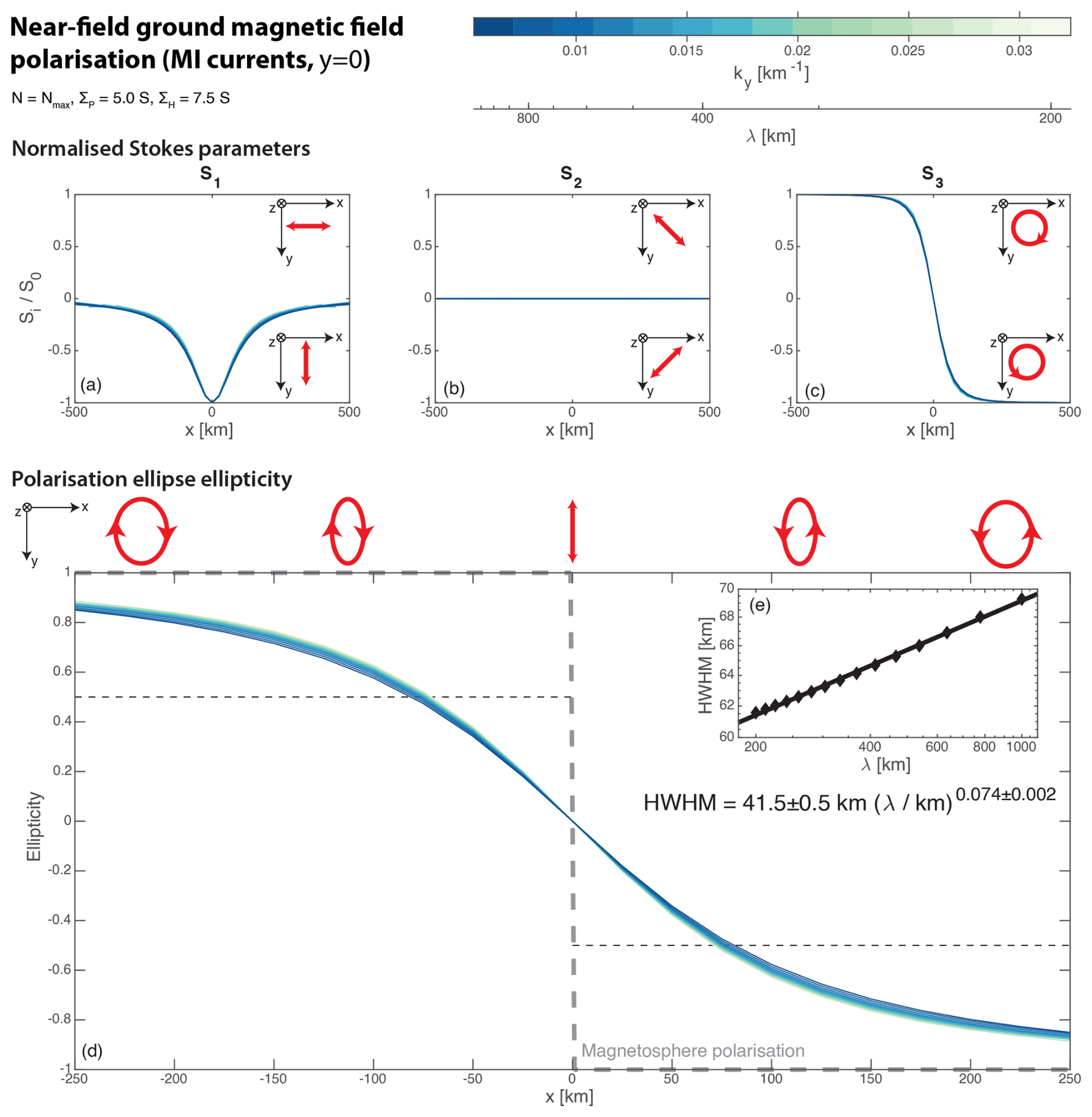
Figure 9Characterising the external ground magnetic field horizontal polarisation for pseudoinfinite waves. (a–c) The three polarisation Stokes parameters normalised by the local intensity plotted along y=0 for different wavenumbers (colours). Inset diagrams indicate corresponding polarisations for each sign. (d) Ellipticity of the wave polarisation along y=0. (e) Half width at half maximum of the ellipticity as a function of wavelength. The solid line shows a power law fit to the data with the shaded area depicting the 95 % prediction interval.
We quantify the, thus far inferred, variation in the horizontal ground polarisation through the four Stokes (1852) parameters
S0 is the intensity, S1 corresponds to linearly polarized waves aligned with either coordinate axis, S2 relates to linearly polarized waves oriented at 45° to the coordinate axes, and finally S3 is associated with circularly polarised waves (Collett, 2005), as depicted by the red arrows in Fig. 9a–c. The degree of polarisation, , was reassuringly unity to machine precision. Figure 9a–c plots the Stokes parameters normalised by intensity along y=0 for a range of wavenumbers, where we omit values where S0<1 nT2 due to potential numerical errors. Panel (c) shows S2 is negligible, indeed calculating the polarisation ellipse's orientation angle yields zero everywhere, i.e. it is aligned with the x axis. has a minimum of −1 at x=0, demonstrating that near the MPBL the surface wave ground signatures are east–west linearly polarised, and slowly tends towards zero away from the MPBL with only slight wavelength variations. While is zero at the MPBL, it grows in magnitude towards ±1 with distance, again with minor differences across wavelengths. This indicates a reversal in polarisation occurs across the MPBL, as expected for a surface wave. We quantify this reversal through the ellipticity, the ratio of the minor to major axes (or equivalently the tangent of the ellipticity angle) of the polarisation ellipse calculated as , shown in panel (d). This takes values from −1 (right-hand circular polarisation), through zero (linear), up to +1 left-hand circular), where handedness is with respect to the vertical, i.e. looking down on the ground. While this indeed shows a reversal in handedness across the MPBL and linear polarisation at x=0, this transition is gradual unlike in the magnetosphere where the infinitesimal current sheet leads to the discontinuous change indicated by the grey dashed line (Plaschke and Glassmeier, 2011). We quantify the scale over which this transition occurs, which appears to have a small dependence on wavelength, using the HWHM corresponding here to when the ellipticity crosses ±0.5 as indicated by the dotted horizontal lines. The inset panel (e) shows the HWHM to be ∼60–70 km, much smaller than typical ground magnetometer spacing and even comparable to those of localised magnetotelluric survey arrays (Archer et al., 2024a). As with the amplitudes, the ellipticity's HWHM follows a power law, though the exponent is rather small explaining why the dependence with wavelength is weak. The exponent is comparable to the difference in exponents of the two horizontal components' amplitude HWHM. It is worth noting that while the ellipticity has only a weak wavelength dependence, the scale over which the ellipticity changes is comparable to that of the amplitude for smaller-scale waves meaning the polarisation on the ground never appreciably reaches that in the magnetosphere. Therefore, as previously inferred, the ionosphere significantly modifies the polarisation of surface waves on the ground from that in the magnetosphere. This was qualitatively mentioned in the global MHD simulation of Archer et al. (2023), though the magnetometer output-resolution was insufficient to resolve the scale over which transitions in polarisation occurred across the ground. This result is not expected for infinite plane waves (Hughes and Southwood, 1976), hence is another example of how breaking this assumption leads to more complicated wave behaviour on the ground.
We tested all these results for pseudoinfinite waves against finite wave packets also (e.g. Fig. 6). After the fluctuations were extracted by the spline-based filtering, we found the ground fields agreed very well with the pseudoinfinite wave results, particularly when close to the centre of the wave packet. This is likely a result of the fluctuating part of the ionospheric currents for finite waves also being well approximated by the infinite wave case, as was shown earlier. Consequently, we have completed a comprehensive characterisation of magnetopause surface waves' ground magnetic field in our model when considering only MI-currents.
4.2.2 Magnetic field (telluric currents)
We use CIM to calculate the contribution to the ground magnetic field from induced telluric currents, which only depends on the skin depth (Eq. 10). While skin depth varies with two model inputs, surface wave frequency and ground conductivity, we only need consider ground-induced effects over a representative range of skin depths. Figure 10 indicates how skin depth varies with both conductivity and frequency, where typical ranges for different ground types and wave phenomena are also given. This shows that magnetopause surface eigenmodes' (MSE) low frequencies (Archer and Plaschke, 2015) result in skin depths much larger than the ionospheric altitude, making telluric current contributions likely small for most ground types as previously commented by Archer et al. (2023). In contrast, telluric currents may be more important for Kelvin–Helmholtz waves, due to higher frequencies, as skin depths become comparable to h. Finally, the well-known phenomenon that the presence of salt water greatly affects ground magnetic field observations is apparent in this figure given skin depths of only a few kilometers across all frequencies.
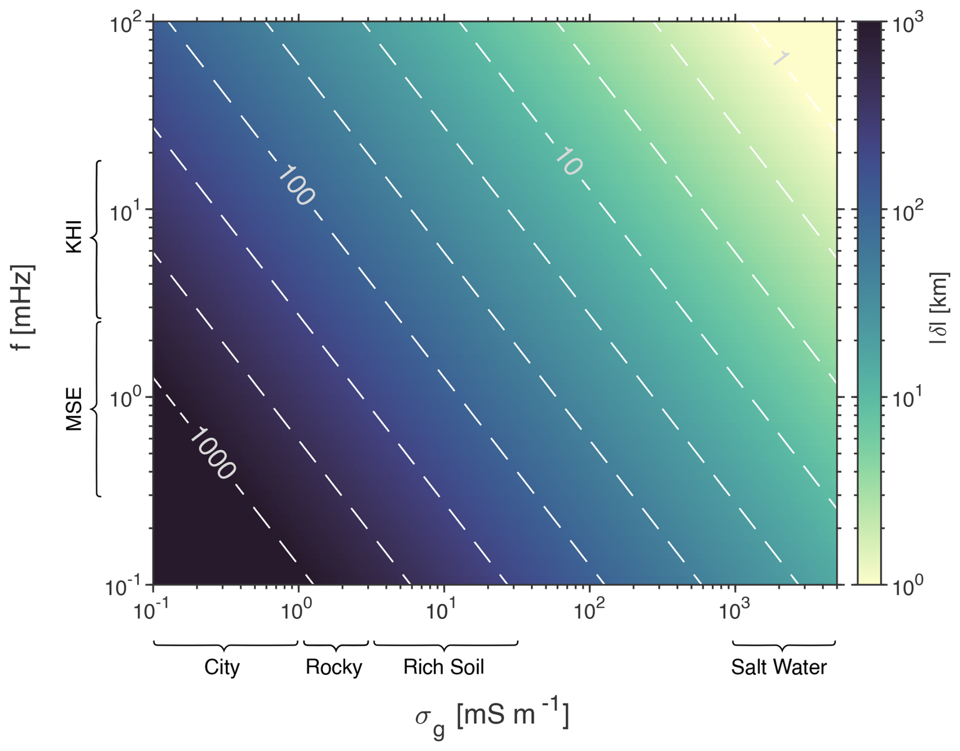
Figure 10Variation of skin depth magnitude with ground conductivity and surface wave frequency depicted as both colours and logarithmically-spaced contours. Ranges of typical conductivities and frequencies for different ground types and magnetopause surface wave phenomena, respectively, are also indicated.
CIM assumes oscillatory currents, which introduces differences between propagating and stationary surface wave packets. With stationary waves all perturbations oscillate in time. However, only the periodic fluctuations are oscillatory for propagating waves, since background trends lead to much slower temporal variations as the wave packet propagates with speed . Our implementation of CIM does not take this into account, simply integrating over all currents within the model. However, given our model is linear with dispersionless waves, we can spatially filter following CIM to correct the internal ground magnetic fields for propagating waves. The results for a finite wave packet are shown in panels (d)–(e) and (k)–(l) of Fig. 6. Amplitudes of fluctuations are identical between propagating and stationary waves, with a 90° phase difference present. However, since the trends also contribute for stationary waves they have significantly larger internal field contributions, which to our knowledge has not been suggested before. While these finite wave effects appear much larger than the fluctuations in the near-field, we leave modelling them to future work focusing only on pseudoinfinite propagating waves.
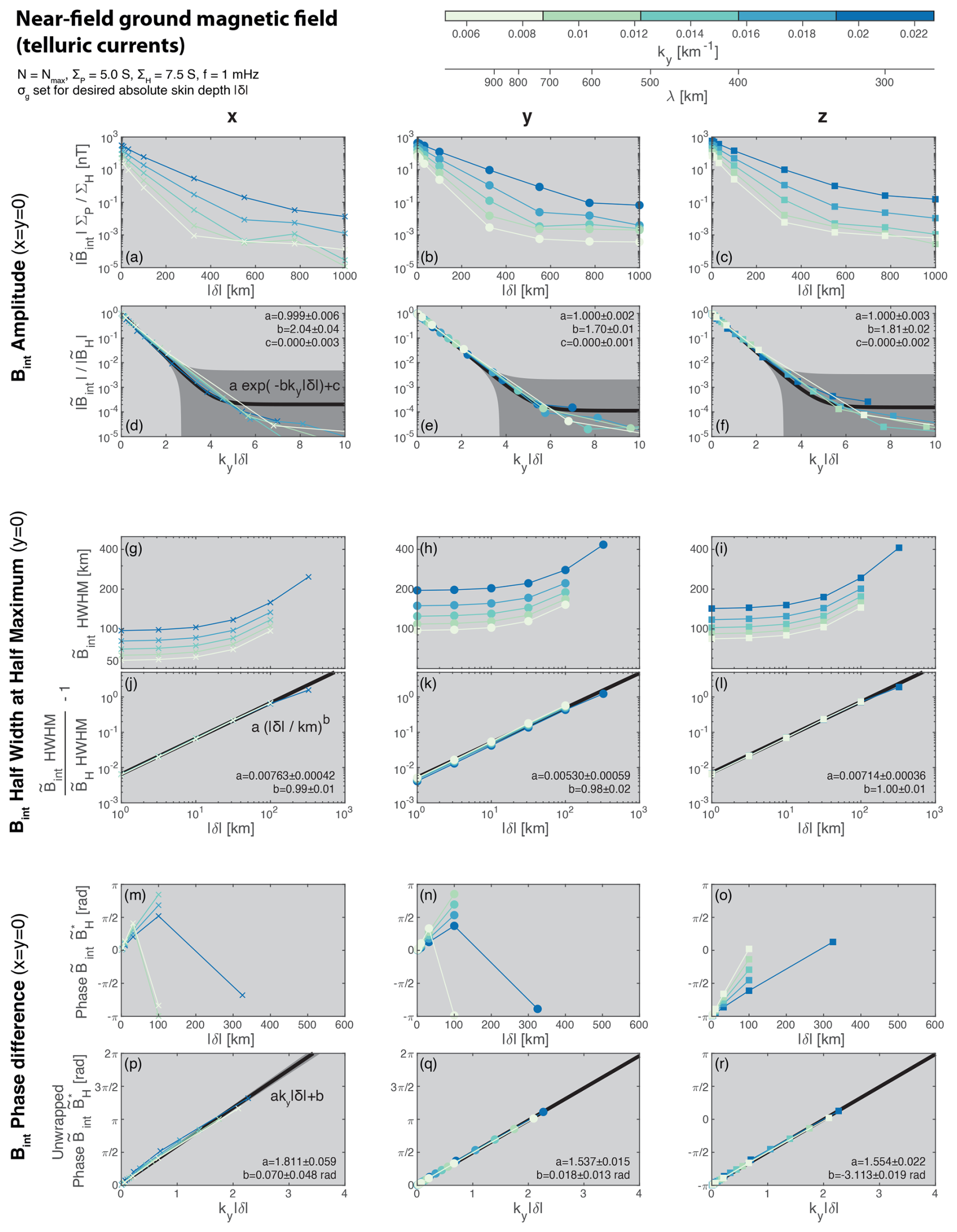
Figure 11Characterising the induced ground magnetic field for pseudoinfinite propagating waves as a function of skin depth for different wavelengths (colours). A similar format of pairs of rows to that in Fig. 5 is used. The top rows (a–c, g–i, m–o) show the model output, whereas bottom rows (d–f, j–l, p–r) normalise results based on the external ground magnetic field such that curves collapse on to one another. Empirical fits (black) and their 95 % prediction intervals are also shown for these normalised results. Columns depict results for each magnetic field component separately. (a–f) Amplitudes at x=0. (g–l) Half width at half maximum along the x axis. (m–r) Phase difference from the external ground field at x=0.
Figure 11a–c show internal magnetic field amplitudes of the three components on the ground as a function of skin depth for five different wavelengths. As before, the x component corresponds to an analytic envelope. All three components appear to follow exponential decays with different decay constants for each wavelength. However, as the field becomes small results level off, suggesting numerical errors begin to dominate. We wish to normalise these curves on to one another in order to characterise the response. An obvious choice of normalisation for the distance is the wavenumber, as used previously. For the amplitude though, we recognise in the limit of infinite ground conductivity (zero skin depth) all components of the internal field must be equal in magnitude to that from Hall currents. This is because in a perfect conductor the induced currents act to cancel out the vertical magnetic field at the surface, in turn doubling the horizontal field. Therefore, we divide the internal field amplitudes by those due to Hall currents, with the results shown in panels (d)–(f). This succeeds at normalising the numerical results onto one another and we fit an exponential decay law to all normalised data. While the amplitudes and offsets from the three fits are consistent with unity and zero, respectively, we again find decay coefficients differs for each component.
We next investigate the HWHM along x for each component. Given numerical errors for large skin depths, we only consider when the ratio of internal to Hall amplitudes was greater than (cf. Fig. 11d–f). The results in Fig. 11g–i show in the limit of zero skin depth the HWHM plateau to a minimum value (different for each wavelength), while as the skin depth increases so too do the HWHM. This makes sense as in CIM image Hall currents get placed further away from the ground as the skin depth increases, thereby widening the scale of their ground signatures. The minimum HWHM should, for similar reasons as the amplitude, be equal to that due to Hall currents, therefore, in panels (j)–(l) we plot the ratio of the two scales minus one. Given the HWHM for the Hall currents followed a power law, we show a log–log plot of this normalised HWHM against skin depth. This again causes the different wavelength curves to collapse onto one another and fitting reveals the power law exponent for each component is consistent with unity, i.e. linear relationships.
Finally, we show the phase difference between the internal field and that from Hall currents in Fig. 11m–o, again only when the ratio of the internal to Hall amplitudes was sufficiently large. For small skin depths phase differences are close to zero for the horizontal components and −π for the vertical, as expected in the perfectly conducting limit. As skin depth initially increases, so too do the phase differences, though at different rates for the various wavelengths with this being greater for larger wavelengths. Normalising the skin depth using the wavenumber and unwrapping the phase, we find in panels (p)–(r) that the phase differences collapse onto one another and appear to follow linear relations.
Similarly to the ground field due to MI-currents, and likely for the same reason, the fluctuating part of the internal field from finite wave packets (Fig. 6) agree well with the infinite wave case. Thus concludes our characterisation of the ground magnetic field contributions due to telluric currents.
4.2.3 Geoelectric field
CIM is again used to calculate the geoelectric field, with example cuts shown in Fig. 6f–g and m–n for both propagating and stationary wave cases. The geoelectric field is generally greatest in the latitudinal x-direction peaking at the MPBL-projection, with the longitudinal component reversing sign across the MPBL and being significantly weaker in amplitude. Like with the ground magnetic field, the geoelectric field has the same amplitudes of periodic fluctuations between both propagating and stationary cases with a 90° phase shift between them (note y=0 is an Eg,y node for stationary waves). Furthermore, stationary waves have significantly larger overall amplitudes due to finite wave effects' contributions, i.e. the trends away from periodic behaviour. Here we focus only on the periodic geoelectric field fluctutations for pseudoinfinite propagating waves.
The geoelectric field depends on both wave frequency and ground conductivity independently, i.e. the dependence cannot be reduced to a single joint parameter. However, like with the induced magnetic field, the vector potential from which the geoelectric field is derived is a function of only skin depth (Eq. 13), meaning for fixed skin depth the quantity is invariant (Eq. 12), simplifying the analysis.
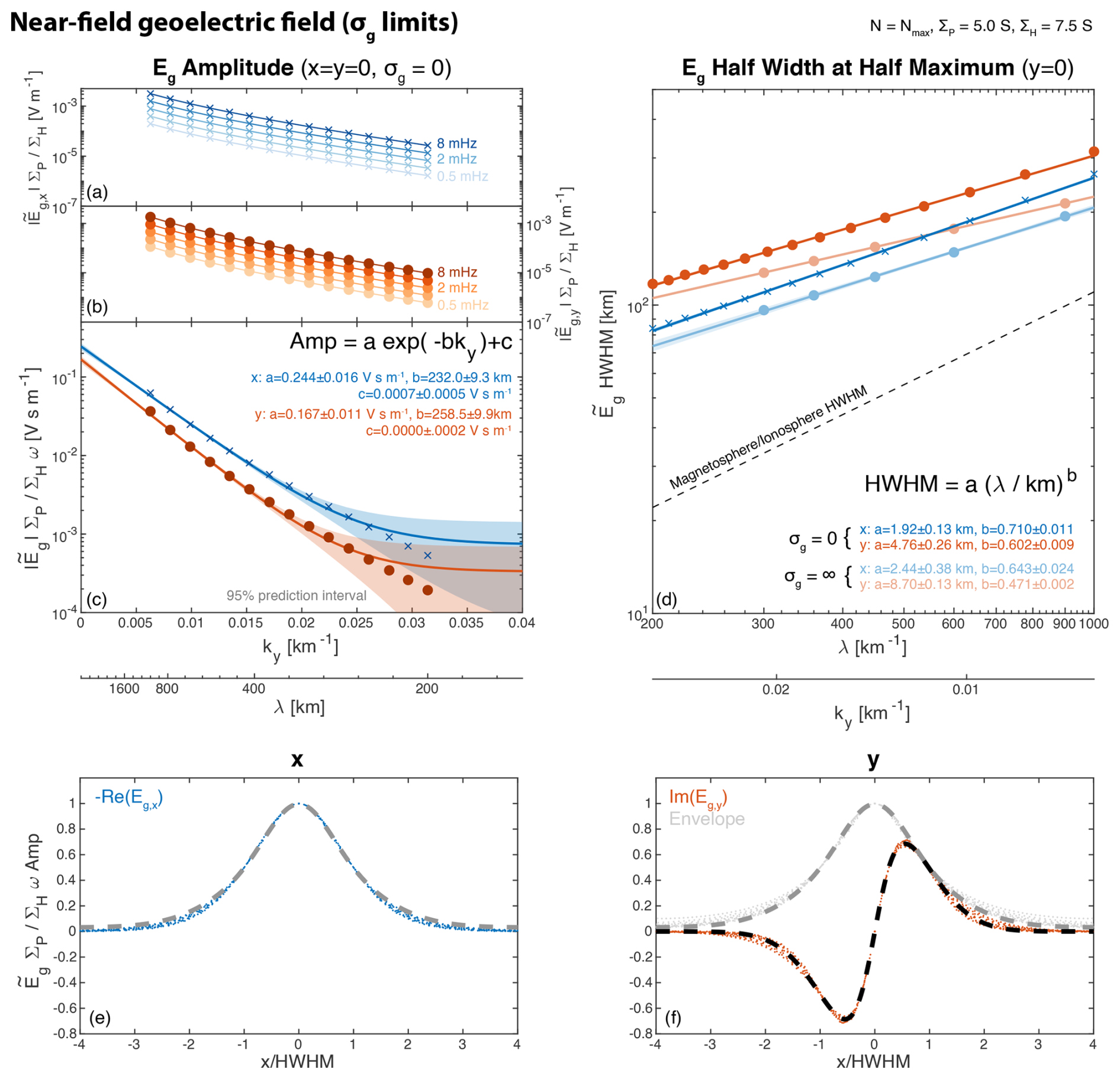
Figure 12Characterising the geoelectric field for pseudoinfinite propagating waves in the limit of zero ground conductivity. Format is similar to Fig. 8. Amplitudes of the x (a) and y (b) electric field components for different surface wave frequencies are depicted by colours, with the frequency-normalised amplitudes shown below (c). Asymptotic limits of the half width at half maximum for infinite ground conductivity is also shown in panel (d) as the lighter colours.
We first consider the zero ground conductivity (infinite skin depth) limit, which will result in the largest geoelectric fields. Figure 12a–b shows how amplitudes of the two geoelectric field components at the MPBL vary with wavenumber for a range of representative frequencies. For the y component an analytic signal envelope has been taken. The amplitude increases with frequency in this limit, demonstrating significant geoelectric fields of up to several mV m−1 may be possible, particularly for large-scale waves and higher frequencies. Both components show approximately exponential decay with wavenumber, which is parameterised in panel (c) where the wave frequency and ionospheric conductance ratio dependences have been removed. The e-folding scale is different for the two components and is significantly greater than both the ionospheric altitude and the e-folding scales of the ground magnetic field. The HWHM again appears to follow a power law with wavelength, with the scales of the geoelectric field again being greater than that in the magnetosphere/ionosphere as well as that of the ground magnetic field, being in the range ∼80–300 km. This highlights that the local is insufficient in prescribing the geoelectric field for mesoscale phenomena. The longitudinal geoelectric field, Eg,y, while weaker in amplitude is the more widespread geoelectric field component. In panels (e)–(f) all profiles are normalised by their respective amplitudes and HWHM. Curiously, the geoelectric field follows the same normalised profile as the ground magnetic field. This is not obvious mathematically as while the geoelectric field is derived from the same current distribution, the weighting by distance of these currents is different.
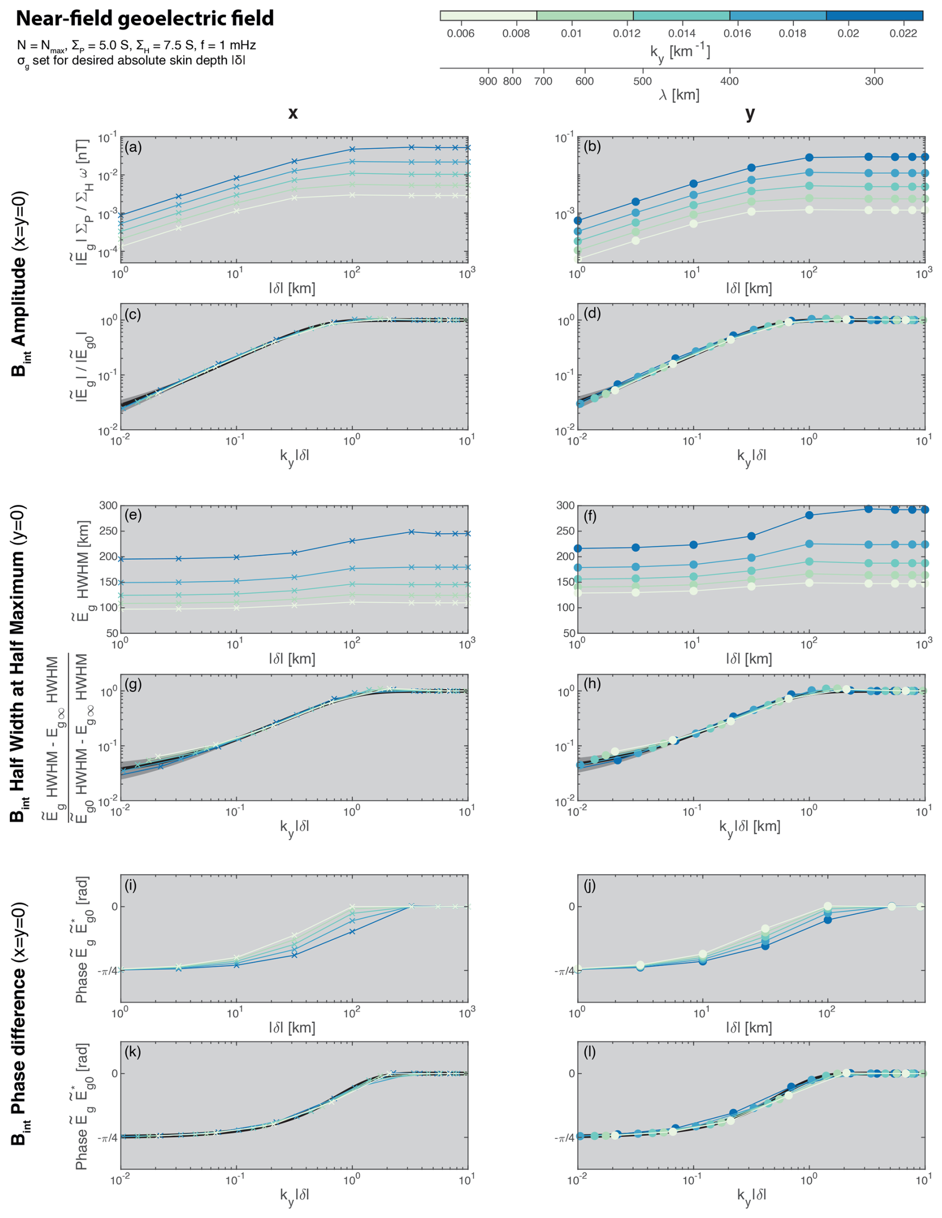
Figure 13Characterising the geoelectric field for pseudoinfinite propagating waves as a function of skin depth for different wavelengths (colours) in a similar format to Fig. 11. Subscripts of zero and infinity refer to the ground conductivity limits. Illustrative fits (black) use a sigmoid-shaped function.
Having characterised the geoelectric field for the limiting case of zero ground conductivity, and knowing that infinite ground conductivity will yield no geoelectric field, we wish to understand the transitional behaviour between these limits. As intimated earlier, we do this by normalising the geoelectric field by the frequency and conductance ratio such that the result is only dependent on skin depth. We first investigate amplitudes, which are shown in Fig. 13a–b for the two components as a function of skin depth. This shows for small skin depths the geoelectric field is small, but as skin depth increases it quickly rises in magnitude. Once the skin depth becomes of order of the ionospheric altitude the geoelectric field plateaus towards the wavelength-dependent zero ground conductivity limits. We find in panels (c)–(d) that normalising the geoelectric field to its aysymptotic limit and the skin depth by the wavenumber causes all the curves to collapse onto a single sigmoid-shaped function.
Next we investigate the HWHM perpendicular to the MPBL. Panels (e)–(f) show this transitions between a slightly smaller scale for zero skin depth (infinite ground conductivity) to a larger one for infinite skin depth (zero ground conductivity), both of which vary with wavelength. While we have already parameterised the latter, the former cannot be ascertained directly as zero skin depth corresponds to no geoelectric field. Therefore, we numerically determine the aymptotic HWHM by assuming a geometric series, found to hold well for the smallest three skin depths shown. The results are displayed in Fig. 12b as the lighter colours. While the HWHM for infinite ground conductivity also follow power laws in wavelength, these have different coefficients and exponents to the zero ground conductivity case. In Fig. 13g–h we subtract this HWHM offset and divide by the difference in HWHM between the ground conductivity limits to yield normalised HWHM between zero and one. When also normalising the skin depth by the wavenumber the curves collapse onto another sigmoid-shaped form.
Finally, we compare the phase differences between the geoelectric field for finite skin depth and that in the limit of zero ground conductivity (infinite skin depth), as shown in Fig. 13i–j. While as expected these all tend towards zero for large skin depth, there is also a wavelength-independent limit for small skin depths of . However, how quickly the phase converges on these limits is wavelength-dependent. Normalising the skin depth through the wavenumber again causes the data to collapse onto a single curve for each component.
Again, finite waves' fluctuations (Fig. 6) show good agreement with the infinite wave case. We, therefore, have fully parameterised the geoelectric field due to magnetopause surface waves.
5.1 Summary
We have performed a comprehensive characterisation of expected effects of mesoscale magnetopause surface waves (ionospheric wavelengths ranging 200–1600 km) within the ionosphere and on the ground using a highly simplified local numerical model, detailing how the response's amplitudes and spatial scales vary with key wave and system properties. We have focused on the near- and far-field limits of finite constant-amplitude sinusoidal wave packets of limited extent, motivated by the existence of both quasi-continuous (e.g. Fairfield et al., 2000; Viall et al., 2009) and impulsive (e.g. Shue et al., 2009; Kozyreva et al., 2019) surface wave drivers. These have resulted in numerous novel insights into the problem of surface wave coupling across the MIG system. We summarise the major findings of this study:
- 1.
Finite surface wave packets' ionospheric and ground signatures can be described as the sum of periodic fluctuations and slowly-varying background trends.
- a.
Within the wave packet, fluctuations are modulated sinusoids along the wave vector direction with the same wavelength as the original surface wave, which are not present far outside the wave packet longitudinally.
- b.
Trends are a result of the finite nature of the wave packet, as imbalances in source terms on either side along the wave vector direction result in imperfect cancellation.
- c.
These trends for finite wave packets introduce differences in effects for propagating and stationary surface waves. With propagating waves, trends cause slower-than-ULF time variations meaning only the fluctuations contribute to the geoelectric field and ground-induced contribution to the surface magnetic field. In contrast, for stationary waves the trends also oscillate at the surface wave frequency, leading to larger overall amplitudes in both quantities.
- a.
- 2.
Close to the wave packet (the near-field) ionospheric fluctuations agree well with theory for an infinite surface wave when is small, showing exponentially decaying signatures with latitudinal distance from the projected Magnetopause Boundary Layer (MPBL) flux tubes. Outside the wave packet where is large (the far-field), surface waves acts as a localised string of field-aligned current sources causing large-scale ionospheric electrodynamics. Their influence on the ionosphere and ground magnetic field can be described as a two-dimensional current dipole, where the dipole moment is larger for greater surface wave amplitudes, wavelengths, and number of oscillations.
- 3.
The relationship between the magnetic field above and below the ionosphere becomes more complicated for surface waves than infinite plane Alfvén waves (Hughes, 1974; Hughes and Southwood, 1974, 1976) due to interference patterns between the spectrum of wavenumbers introduced by the additional spatial wave structure.
- a.
The ionosphere similarly screens small-scale surface waves from the ground, however the e-folding scale (which varies with each component of the field) of this effect with azimuthal wavenumber is larger than the ionospheric altitude, likely due to a spectrum of total wavenumbers present.
- b.
While the rotation of the ground magnetic field is on average close to (but not exactly) 90°, significant spread in rotation angles occurs spatially. Instances of the opposite rotation sense also occur periodically along the MPBL-projection.
- c.
The ionosphere significantly modifies the polarisation of the surface wave, only gradually transitioning between handedness across the MPBL-projection, unlike the discontinuous change in the magnetosphere. For smaller wavelengths this means ground-observed polarisations may never match that in space.
- a.
- 4.
Surface wave effects are highly localised latitudinally. While in the ionosphere their latitudinal scales vary linearly with wavelength as in the magnetosphere, the Half Width at Half Maxima (HWHM) for the ground fields appear to instead follow power laws with exponents that differ by component.
- a.
Ionospheric HWHM range ∼20–175 km meaning even relatively large-scale surface waves should have very concentrated impacts latitudinally.
- b.
Ground magnetic field HWHM, though larger than in the ionosphere and magnetosphere, are comparable to or smaller than typical spacings of ground magnetometer chains for even large wavelength surface waves at ∼100–200 km.
- c.
Ground magnetic polarisation changes occur over distances comparable to the spacings of even localised magnetotelluric survey arrays at ∼60–70 km.
- d.
Geoelectric field scales are larger than those of the ground magnetic field at ∼80–300 km, highlighting that local is insufficient in prescribing the geoelectric field for mesoscale phenomena.
- a.
- 5.
Inductive effects in the ground and their contribution to the ground magnetic and geoelectric fields depend on the magnitude of the wavenumber multiplied by the skin depth, i.e. . Across the ranges of wavenumbers and skin depths applicable to magnetopause surface waves, the ground can act either like:
- a.
A perfect insulator (), where the vertical component of the ground magnetic field acts a strong detector of surface wave's FACs and geoelectric fields are maximised.
- b.
A perfect conductor (), where telluric currents cancel the vertical component of the magnetic field, double the horizontal ground field components, and no geoelectric field is induced.
- c.
A finite conductor, where properties smoothly transition between the above limiting cases with normalised skin depth .
- a.
- 6.
The predicted amplitudes of magnetopause surface wave effects suggest they may act as a significant, but highly latitudinally localised, source of Joule heating in the ionosphere (up to hundreds of mW m−2) and the geoelectric fields (up to several mV m−1) that drive geomagnetically-induced currents, particularly for large-scale waves, thereby contributing to space weather impacts.
5.2 Limitations
These results have been determined from a deliberately simple local numerical model, enabling such comprehensive characterisation of how surface wave effects may vary with key wave and system parameters. However, as we outlined from the outset, the simplicity of this model is designed to enable initial physical insight and intuitive understanding to the coupling of surface waves across the MIG-system. It is, therefore, important to consider the validity of the model assumptions along with outlining further refinements that could test incorporating more realistic effects in the future to iterate these results.
We have used a box model magnetosphere with vertical field lines. While we justified this does not affect current amplitudes at the MI-interface, meaning that ionospheric current systems are reliable, the assumption may affect the ground fields that integrate the magnetospheric currents. Our results for the ground fields pertain solely to ionospheric Hall currents and should only be treated as such. This is because Fukushima's (1976) theorem was shown to be a good approximation due to the model setup. In reality though this approximation is only considered reasonable for high-latitudes (Untiedt and Baumjohann, 1993; Laundal et al., 2015) and, in general, one would also expect a contribution due to the non-cancellation of magnetospheric and Pedersen currents, with several factors to consider. Firstly, the field-aligned phase variation in our model is linear with distance. However, inhomogeneity in magnetic field and plasma condition along field lines may modify parallel wave structure. Archer and Plaschke (2015) demonstrated surface wave phase speeds are significantly larger close to Earth, primarily due to the dipole field, such that very slow phase variation are expected along the field. Even in our simple model the ground fields were insensitive to field-aligned phase variations, given and currents closest to Earth dominate the Biot–Savart law (only 5 % of the ground field contribution arises from magnetopause currents above ∼0.7–4 RE, dependent on wavelength). Thus one might similarly expect little sensitivity to slow field-aligned phase variations, though this could be checked. Secondly, current density variations along field lines are also expected due to the changing area of flux tubes along the field, not accounted for in a uniform field. Given the product of the current density and flux tube area, jdA, remains invariant along flux tubes though, this aspect of the Biot–Savart integrand is little affected to a first approximation. However, the magnetic geometry does alter the integrand via the position vectors. Fukushima (1976) outlines a correction term for realistic geometries using an additional current system along these magnetic field lines and cancelling out the vertical ones. Examining this correction for surface waves and its dependence on latitude and wavelength should be investigated.
In our model we only consider wavelengths up to of order the distance to the horizon from ionospheric altitude, for which the Cartesian model used is appropriate. For larger wavelengths a spherical model would likely be required, which again would introduce latitudinal-dependence to results.
We justified using magnetopause currents with infinitesimal width in terms of the ionospheric currents outside the thin boundary layer projection. A simple modification to account for finite thickness is to linearly interpolate ionospheric currents in the range , corresponding to a uniform magnetopause current layer of typical thickness d∼40 km at the ionosphere. Given the highly localised ionospheric response, maxima in the ionosphere become significantly capped for small-scale waves (by ∼50 % for 200 km wavelength), whereas large-scale waves are little affected. In terms of the ground field fluctuations, we find accounting for the boundary thickness overall rescales the entire perturbation strengths by a factor of order , i.e. less than a 20 % reduction for small-scale waves, and does not seemingly affect the HWHM or latitudinal-form. Background trends also remain unaffected. While in reality the current layer is likely not uniform, instead exhibiting a peak near the inner/equatorward edge (Archer et al., 2023), a uniform current layer provides the maximum possible difference in results from our assumed infinitesimal layer when considering boundary layer structure.
The magnetopause surface waves currents were derived from Ideal MHD (Plaschke and Glassmeier, 2011). Therefore, we include no parallel electric fields between the magnetosphere and ionosphere. The result was FAC amplitudes independent of wavelength. Johnson et al. (2021), in contrast, employed a linear Knight (1973) relation in their MI-coupling, finding a nonlinear Kelvin–Helmholtz vortex size which maximises FACs. Following the framework of Yoshikawa et al. (2011), it can be shown in our model for dusk-sector linear waves with small current amplitudes (compared to the background Region-1 currents) the FAC amplitude is slightly modified becoming , where κ is the Knight parameter. The resistive-coupling auroral scale length is typically ∼50 km (Lyons, 1980), implying auroral acceleration should not significantly modify linear surface wave results for the wavelengths presented. If the resistive-coupling length scale becomes comparable to or larger than the wavelength, so long as the linear regime still holds our results are only slightly modified given the predicted current amplitude modulation is weaker than the exponential and power law dependencies on wavenumber already found. However, if waves become nonlinear and/or develop into rolled-up vortices, then the parallel electric field likely would become important to the wave coupling, requiring a different approach.
While a uniform magnetic field and plasmas were employed in each half-space, perpendicular non-uniformities in the magnetic field or plasma necessarily couple compressional waves to Alfvén modes throughout the magnetosphere (Radoski, 1971). Archer et al. (2023) showed in high-resolution global MHD simulations this leads to additional FACs on closed field lines throughout the magnetosphere that contribute to the ionospheric and ground responses, which our model does not capture. Nonetheless, the simulation showed FAC amplitudes exhibited distinct peaks within the projection of the magnetopause boundary layer, with those from the non-resonant coupling being around an order of magnitude weaker. Therefore, one might expect the overall response to be dominated by the magnetopause currents that our model does capture. Future work could investigate introducing these additional currents and their effects.
Only uniform ionospheric conductances were used. It is known that solar illumination and auroral precipitating particles contribute to the spatial distribution of conductances (Ridley et al., 2004), which will affect current patterns. Sunlight effects result in small variations over scales comparable to the planet's surface, i.e. much larger than a surface mode wavelength, hence will likely have little effect on predictions. The auroral oval typically has a latitudinal width of 10–17° (Walach et al., 2017), i.e. of similar size to or greater than the model domain and thus larger than the scales of surface waves considered. Proportional changes in conductance are also typically smaller on the dayside than the nightside (Ridley et al., 2004). This suggests mesoscale dayside currents due to surface waves might be little affected by the additional auroral conductance. Laundal et al. (2015) also argue that at the dayside polar cap boundaries ionospheric conductance gradients are approximately perpendicular to equipotential contours, meaning only Hall currents should contribute to the ground magnetic field as per Fukushima (1976). Further work could modify the model to include conductance gradients and investigate their effects on surface waves over different scales.
We have also only considered uniform ground conductivities, which results in a simple relationship for the skin depth in terms of both wave frequency and conductivity. However, CIM can also be used for vertically-varying ground conductivities, i.e. a multi-layered Earth (Thomson and Weaver, 1975). In this case, the effective skin depth used in CIM for placing image currents becomes altered from the uniform case with a more complicated frequency dependence. Since we showed our results for surface waves are a function only of the skin depth, they can readily be applied to these cases also. However, where three-dimensional conductivities are thought to be important (e.g. Bedrosian and Love, 2015) a full inductive treatment would likely be required (Weaver, 1971).
Finally, our model contains no self-consistent dissipation, nor additional non-Ideal physics such as ionospheric viscosity (Yerg, 1952), turbulence (Guio and Pécseli, 2021), or kinetic plasma effects (e.g. Hasegawa, 1976; Lee et al., 1994). This means amplitudes presented are likely overestimates. In contrast, global MHD simulations usually suffer from strong numerical diffusion artificially damping waves and smearing their effects over larger scales (Claudepierre et al., 2009; Hartinger et al., 2015b), leading to underestimates. Given the large amplitudes and short scales predicted from this simple model, it is clear future simulations using numerical schemes and grid geometries that limit diffusion at the magnetopause/cusps (e.g. Sorathia et al., 2017; Zhang et al., 2019) run at even higher spatial resolution throughout the magnetosphere, ionosphere and on the ground are required to better test results derived from such a simple model against a much more representative environment.
5.3 Implications
The results presented in this work provide insight into the ionospheric and ground-based impacts magnetopause surface waves may have, particularly how their amplitudes and spatial scales may vary. Archer et al. (2024a) recently laid out future observational directions for unveiling magnetopause dynamics and their geospace impacts, with the wealth of current ground-based instrumentation being highlighted in particular. Correctly interpreting ground-based measurements as being due to magnetopause surface waves though requires comprehensive theoretical underpinning. Reanalysis of previously examined events in light of this work is thus needed, as well as dedicated future campaigns taking advantage of recent and upcoming capabilities.
Doppler radars, such as the SuperDARN network (e.g. Nishitani et al., 2019), provide measurements of the line-of-sight component to the ionospheric velocity. Historically ULF wave studies have been limited to measurements from a single radar (e.g. Fenrich et al., 1995) due to ∼1–2 min full scan time. However, SuperDARN's range gates have typical spatial resolution ∼45 km (Chisham et al., 2007), similar to surface waves' latitudinal scales for smaller wavelengths (∼200–400 km at the MI-interface, ∼1–2 RE at the equatorial magnetopause, m∼30–70). It is thus questionable whether SuperDARN might resolve these features. The discretionarily-available “myopic” mode can provide ∼15 km resolution but with smaller field-of-view (Lester et al., 2004) and may be required for dedicated surface wave studies. On the other hand, availability of only the line-of-sight velocity component is limiting since the look direction might not always be best aligned with wave phenomena or provide sufficient discrimination against different wave modes. Ongoing upgrades to the SuperDARN network to digital systems are now enabling full scans over only 3.5 s, which removes the restriction of only single radar (McWilliams et al., 2023). While typical spatial resolution is unchanged, the higher ∼15 km resolution is also still available. Therefore, it may soon be possible, thanks to overlapping fields-of-view from different digital radar and applying high-order local/regional fitting (Fenrich et al., 2019), to reconstruct the ionospheric convection vortices and current dipole patterns of magnetopause surface waves, though this would likely need to be as part of a dedicated campaign. The ability, or not, of radar to resolve surface waves' ionospheric effects has implications not only on remote sensing magnetospheric processes, but on overall estimates of Joule heating in the ionosphere/thermosphere and hence global space weather. Hurd and Larsen (2016) previously estimated small-scale fluctuating ionospheric electric fields, poorly resolved by radar measurements, might contribute more than twice the contributions to Joule heating of the large-scale steady fields. Our model suggests magnetopause surface waves could be a significant source of highly latitudinally-localised oscillatory Joule heating. This strengthens the need for high spatio-temporal resolution ionospheric coverage to better understand how mesoscale phenomena contribute to global MI-coupling and space weather (Heelis and Maute, 2020; Pakhotin and Mann, 2024).
Our ground magnetic field results suggest mesoscale structures, like magnetopause surface waves, can have significant amplitudes but may be poorly resolved by the typical spacing of ground magnetometer networks. This may be why conclusive ground-based evidence for surface modes has proven challenging (Pilipenko et al., 2017, 2018; Kozyreva et al., 2019). These results come from a simple homogeneous model, without the complication of spatially-varying ground conductivities that are often invoked when closely-spaced (<100 km) magnetometers measurements differ (e.g. Juusola et al., 2020; Shi et al., 2025b). Our work, therefore, motivates the need for denser networks of ground measurements in order to identify the polarisation and wave power variations predicted. Another possibility might be placing magnetotelluric survey networks, smaller dense arrays taking simultaneous geoelectric and geomagnetic field measurements (Hartinger et al., 2020; Shi et al., 2022), close to the expected position of the OCB as part of dedicated campaigns. Our work has also highlighted the value of studying the vertical component of the ground magnetic field. Firstly, this component acts as a clear signifier of field-aligned currents, when ground inductive effects can be neglected. However, given for surface waves the expected horizontal and vertical field components are of comparable magnitude, this suggests that the ratio of the vertical to horizontal components' amplitudes could be used as a measure of the relative contribution of ground induction in ground-based magnetic field observations.
The ESA/CAS Solar Wind Magnetosphere Ionosphere Link Explorer (SMILE) mission aims to image the dayside magnetopause in soft X-rays, intending to uncover the fundamental modes of the dayside solar wind–magnetosphere interaction through near-continual remote sensing (Wang et al., 2025). While signal-to-noise is expected to be difficult under typical driving, it is hoped large-scale magnetopause motion such as directly-driven surface waves might be resolvable (Connor et al., 2025), though this may require advanced processing techniques (Archer et al., 2024a). As part of the SMILE mission, coordinated efforts to complement space-based measurements with ground-based instruments are being undertaken (Carter et al., 2024), including software tools for planning dedicated ground-based campaigns (Walach et al., 2024). These might address open science questions such as the scale sizes and structuring of ULF oscillations in the ionospheric cusp region and how these map out and relate to wave phenomena in space, such as magnetopause surface waves. Near-continual remote-sensing of magnetopause surface waves in soft X-rays with simultaneous conjugate measurements of the ionosphere and ground would likely provide the best test of these theoretical results, eliminating the need for rare in situ conjunction events.
Finally, the framework and scope of the numerical model presented here might be extended. Plasmapause surface wave (Chen and Hasegawa, 1974; He et al., 2020) impacts require only scaling some of the fixed model parameters, therefore, many of the results already presented might be readily applied. Adjusting the form of the currents in the magnetosphere to other mesoscale, time-varying phenomena, e.g. field line resonances (Southwood, 1974; Wright and Elsden, 2020) or flux transfer events (Lee and Fu, 1985), would enable them to be studied in a comparative way to better understand the different sources of ionospheric and ground perturbations in general, as well as their relative importance within the context of space weather.
Here we describe a spline-based filtering method for splitting data, a(y), from our model into periodic fluctations, , plus a background trend, 〈a(y)〉. It was inspired by Empirical Mode Decomposition (EMD; Huang et al., 1971), which algorithmically decomposes non-stationary, non-linear data into well-behaved oscillatory components plus a non-oscillatory residual/trend. Our filtering method, depicted in Fig. A1, is performed along the y-direction only, where the periodicity of fluctuations is known a priori to be λ (a marked difference from EMD where such information is not known). For a given starting position, points of the same phase, i.e. separated by λ, are Akima (1970) spline interpolated across (red line in Fig. A1a). The same is performed for points in antiphase, i.e. distance from the originals (blue). The midpoint of this pairs of interpolants are an estimate of the background trend (green). For increased robustness, this procedure is repeated across different starting points (we use 16 equally-spaced points between ), with the background trend defined to be the average over all resulting midpoints (Fig. A1b). It follows that the fluctuations are then the difference between the original data and the trend (Fig. A1c).
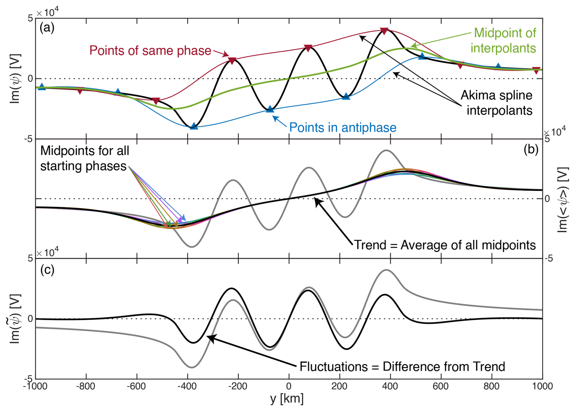
The original contributions presented in the study are publicly available. The software for generating the data can be found at https://doi.org/10.14469/hpc/15489 (Archer, 2025).
MA: Conceptualization, Data curation, Formal analysis, Funding acquisition, Investigation, Methodology, Software, Supervision, Validation, Visualization, Writing – original draft. DS: Formal analysis, Writing – review and editing. SZ: Methodology, Validation. QS: Methodology, Validation. MH: Methodology, Writing – review and editing.
The contact author has declared that none of the authors has any competing interests.
Publisher's note: Copernicus Publications remains neutral with regard to jurisdictional claims made in the text, published maps, institutional affiliations, or any other geographical representation in this paper. The authors bear the ultimate responsibility for providing appropriate place names. Views expressed in the text are those of the authors and do not necessarily reflect the views of the publisher.
MA would like to thank the members of International Space Science Institute (ISSI) Bern International Team project #546 “Magnetohydrodynamic Surface Waves at Earth's Magnetosphere (and Beyond)” for fruitful discussions surrounding this research. The work benefited from use of the Imperial College Research Computing Service (https://doi.org/10.14469/hpc/2232, Imperial College, 2025).
MA was supported by UKRI (STFC/EPSRC) Stephen Hawking Fellowship EP/T01735X/1, UKRI Future Leaders Fellowship MR/X034704/1, and International Space Science Institute (ISSI) Bern International Team project #546 “Magnetohydrodynamic Surface Waves at Earth's Magnetosphere (and Beyond)”. MH was supported by NERC grant NE/V003070/1 and Schmidt Science Fellows, in partnership with the Rhodes Trust. DS acknowledges funding from UK Science and Technology Facilities Council Grant ST/W001071/1.
This paper was edited by Nick Sergis and reviewed by Robert Lysak and one anonymous referee.
Abramowitz, M. and Stegun, I. A.: Handbook of mathematical functions: with formulas, graphs, and mathematical tables, Dover Publications Inc., Mineola, New York, USA, ISBN 0486612724, 2000. a, b
Akima, H.: A new method of interpolation and smooth curve fitting based on local procedures, J. ACM, 17, 589–602, https://doi.org/10.1145/321607.321609, 1970. a
Archer, M., Shi, X., Walach, M.-T., Hartinger, M. D., Gillies, D. M., Di Matteo, S., Staples, F., and Nykyri, K.: Crucial future observations and directions for unveiling magnetopause dynamics and their geospace impacts, Front. Astron. Space Sci., 11, 1430099, https://doi.org/10.3389/fspas.2024.1430099, 2024a. a, b, c, d
Archer, M. O.: Magnetopause surface wave magnetosphere–ionosphere–ground coupling code, Imperial [code], https://doi.org/10.14469/hpc/15489, 2025. a
Archer, M. O. and Plaschke, F.: What frequencies of standing surface waves can the subsolar magnetopause support?, J. Geophys Res., 120, 3632–3646, https://doi.org/10.1002/2014JA020545, 2015. a, b, c
Archer, M. O., Hietala, H., Hartinger, M. D., Plaschke, F., and Angelopoulos, V.: Direct observations of a surface eigenmode of the dayside magnetopause, Nat. Commun., 10, 615, https://doi.org/10.1038/s41467-018-08134-5, 2019. a, b, c, d, e
Archer, M. O., Hartinger, M. D., Plaschke, F., Southwood, D. J., and Rastaetter, L.: Magnetopause ripples going against the flow form azimuthally stationary surface waves, Nat. Commun., 12, 5697, https://doi.org/10.1038/s41467-021-25923-7, 2021. a, b, c, d
Archer, M. O., Southwood, D. J., Hartinger, M. D., Rastaetter, L., and Wright, A. N.: How a realistic magnetosphere alters the polarizations of surface, fast magnetosonic, and Alfvén waves, J. Geophys. Res.-Space, 127, e2021JA030032, https://doi.org/10.1029/2021JA030032, 2022. a, b
Archer, M. O., Hartinger, M. D., Rastátter, L., Southwood, D. J., Heyns, M., Eggington, J. W. B., Wright, A. N., Plaschke, F., and Shi, X.: Auroral, ionospheric and ground magnetic signatures of magnetopause surface modes, J. Geophys. Res.-Space, 128, e2022JA031081, https://doi.org/10.1029/2022JA031081, 2023. a, b, c, d, e, f, g, h, i, j, k, l, m, n, o, p, q
Archer, M. O., Pilipenko, V. A., Li, B., Sorathia, K., Nakariakov, V. M., Elsden, T., and Nykyri, K.: Magnetopause MHD surface wave theory: progress and challenges, Front. Astron. Space Sci., 11, 1407172, https://doi.org/10.3389/fspas.2024.1407172, in press, 2024b. a, b, c, d, e
Axford, W. I.: Viscous interaction between the solar wind and the earth's magnetosphere, Planet. Space Sci., 12, 45–53, https://doi.org/10.1016/0032-0633(64)90067-4, 1964. a
Bedrosian, P. A. and Love, J. J.: Mapping geoelectric fields during magnetic storms: Synthetic analysis of empirical United States impedances, Geophys. Res. Lett., 42, 10160–10170, https://doi.org/10.1002/2015GL066636, 2015. a
Belakhovsky, V., Pilipenko, V., Engebretson, M., Sakharov, Y., and Selivanov, V.: Impulsive disturbances of the geomagnetic field as a cause of induced currents of electric power lines, J. Space Weather Spac., 9, A18, https://doi.org/10.1051/swsc/2019015, 2019. a
Berchem, J. and Russell, C. T.: The thickness of the magnetopause current layer: ISEE 1 and 2 observations, J. Geophys. Res., 87, 2108–2114, https://doi.org/10.1029/JA087iA04p02108, 1982. a
Bhattarai, S. K. and Lopez, R. E.: Reduction of viscous potential for northward interplanetary magnetic field as seen in the LFM simulation, J. Geophys. Res.-Space, 118, 3314–3322, https://doi.org/10.1002/jgra.50368, 2013. a
Boteler, D. H. and Pirjola, R. J.: The complex-image method for calculating the magnetic and electric fields produced at the surface of the Earth by the auroral electrojet, Geophys. J. Int., 132, 31–40, https://doi.org/10.1046/j.1365-246x.1998.00388.x, 1998. a
Brenner, A., Pulkkinen, T. I., and Liemohn, M. W.: Solar Wind-Magnetosphere Coupling Under Interim Steady Conditions, J. Geophys. Res.-Space, 130, e2025JA033771, https://doi.org/10.1029/2025JA033771, 2025. a
Bristow, W. A., Sibeck, D. G., Jacquey, C., Greenwald, R. A., Sofko, G. J., Mukai, T., Yamamoto, T., Kokubun, S., Hughes, T. J., Hughes, W. J., and Engebretson, M. J.: Observations of convection vortices in the afternoon sector using the SuperDARN HF radars, J. Geophys. Res.-Space, 100, 19743–19756, https://doi.org/10.1029/95JA01301, 1995. a
Carter, J. A., Dunlop, M., Forsyth, C., Oksavik, K., Donovon, E., Kavanagh, A., Milan, S. E., Sergienko, T., Fear, R. C., Sibeck, D. G., Connors, M., Yeoman, T., Tan, X., Taylor, M. G. G. T., McWilliams, K., Gjerloev, J., Barnes, R., Billet, D. D., Chisham, G., Dimmock, A., Freeman, M. P., Han, D.-S., Hartinger, M. D., Hsieh, S.-Y. W., Hu, Z.-J., James, M. K., Juusola, L., Kauristie, K., Kronberg, E. A., Lester, M., Manuel, J., Matzka, J., McCrea, I., Miyoshi, Y., Rae, J., Ren, L., Sigernes, F., Spanswick, E., Sterne, K., Steuwer, A., Sun, T., Walach, M.-T., Walsh, B., Wang, C., Weygand, J., Wild, J., Yan, J., Zhang, J., and Zhang, Q.-H.: Ground-based and additional science support for SMILE, Earth and Planetary Physics, 8, 275–298, https://doi.org/10.26464/epp2023055, 2024. a
Chandrasekhar, S.: Hydrodynamic and Hydromagnetic stability, Oxford University Press, Oxford, UK, ISBN 978-0226100975, 1961. a, b
Chen, L. and Hasegawa, A.: A theory of long-period magnetic pulsations: 2. Impulse excitation of surface eigenmode, J. Geophys. Res., 79, 1033–1037, https://doi.org/10.1029/JA079i007p01033, 1974. a, b, c, d, e, f
Chisham, G., Lester, M., Milan, S. E., Freeman, M. P., Bristow, W. A., Grocott, A., McWilliams, K. A., Ruohoniemi, J. M., Yeoman, T. K., Dyson, P. L., Greenwald, R. A., Kikuchi, T., Pinnock, M., Rash, J. P. S., Sato, N., Sofko, G. J., Villain, J.-P., and Walker, A. D. M.: A decade of the Super Dual Auroral Radar Network (SuperDARN): scientific achievements, new techniques and future directions, Surv. Geophys., 28, 33–109, https://doi.org/10.1007/s10712-007-9017-8, 2007. a
Claudepierre, S., Wiltberger, M., Elkington, S., Lotko, W., and Hudson, M.: Magnetospheric cavity modes driven by solar wind dynamic pressure fluctuations, Geophys. Res. Lett., 36, L13101, https://doi.org/10.1029/2009GL039045, 2009. a
Cohen, D. and Hosaka, H.: Part II magnetic field produced by a current dipole, J. Electrocardiol., 9, 409–417, https://doi.org/10.1016/S0022-0736(76)80041-6, 1976. a
Collett, E.: Field Guide to Polarization, SPIE press, Bellingham, WA, USA, ISBN 0-8194-5868-6, 2005. a
Connor, H. K., Sun, T., Samsanov, A., Liang, J., Read, A., Li, D., Cucho-Padin, G., Jung, J., Bickner, B., Escoubet, C. P., Forsyth, C., Sembay, S., Sibeck, D., Spanswick, E., Sydorenko, D., and Wang, C.: SMILE Modeling Working Group: Modeling and Analysis of X-ray and Ultraviolet Images of Solar Wind – Earth Interactions, Space Sci. Rev., 221, 46, https://doi.org/10.1007/s11214-025-01172-8, 2025. a
Degeling, A. W., Rankin, R., Kabin, K., Rae, I. J., and Fenrich, F. R.: Modeling ULF waves in a compressed dipole magnetic field, J. Geophys. Res., 115, A10212, https://doi.org/10.1029/2010JA015410, 2010. a
Elsden, T., Southwood, D. J., Allanson, O., Archer, M. O., Hartinger, M. D., and Wright, A. N.: Theory and Modeling of Large Scale Plasmapause Surface Waves, J. Geophys. Res.-Space, 130, e2025JA033830, https://doi.org/10.1029/2025JA033830, 2025. a, b
Fairfield, D. H., Otto, A., Mukai, T., Kokubun, S., Lepping, R. P., Steinberg, J. T., Lazarus, A. J., and Yamamoto, T.: Geotail observations of the Kelvin–Helmholtz instability at the equatorial magnetotail boundary for parallel northward fields, J. Geophys. Res., 105, 21159–21174, https://doi.org/10.1029/1999JA000316, 2000. a, b, c
Fenrich, F. R., Samson, J. C., Sofko, G., and Greenwald, R. A.: ULF high- and low-m field line resonances observed with the Super Dual Auroral Radar Network, J. Geophys. Res.-Space, 100, 21535–21547, https://doi.org/10.1029/95JA02024, 1995. a
Fenrich, F. R., Gillies, D. M., Donovan, E., and Knudsen, D.: Flow Velocity and Field-Aligned Current Associated With Field Line Resonance: SuperDARN Measurements, J. Geophys. Res.-Space, 124, 4889–4904, https://doi.org/10.1029/2019JA026529, 2019. a
Friis-Christensen, E., McHenry, M. A., Clauer, C. R., and Vennerstrøm, S.: Ionospheric traveling convection vortices observed near the polar cleft: A triggered response to sudden changes in the solar wind, Geophys. Res. Lett., 15, 253–256, https://doi.org/10.1029/GL015i003p00253, 1988. a
Fukushima, N.: Generalized theorem for no ground magnetic effect of vertical currents connected with Pedersen currents in the uniform-conductivity ionosphere, Rep. Ionos. Space Res. Jap., 30, 35–40, 1976. a, b, c
Ganushkina, N. Y., Liemohn, M. W., and Dubyagin, S.: Current Systems in the Earth's Magnetosphere, Rev. Geophys., 56, 309–332, https://doi.org/10.1002/2017RG000590, 2018. a
GeoSci.xyz Project: EM GeoSci: A online textbook for electromagnetic geophysics, https://doi.org/10.5281/zenodo.2548027, https://em.geosci.xyz (last access: 19 August 2024), 2015. a
Glassmeier, K.-H.: Traveling magnetospheric convection twin-vortices: observations and theory, Ann. Geophys., 10, 1992. a
Glassmeier, K.-H. and Heppner, C.: Traveling magnetospheric convection twin vortices: Another case study, global characteristics, and a model, J. Geophys. Res.-Space, 97, 3977–3992, https://doi.org/10.1029/91JA02464, 1992. a
Goodman, M. L.: A three-dimensional, iterative mapping procedure for the implementation of an ionosphere-magnetosphere anisotropic Ohm's law boundary condition in global magnetohydrodynamic simulations, Ann. Geophys., 13, 843–853, https://doi.org/10.1007/s00585-995-0843-z, 1995. a
Greenwald, R. A. and Walker, A. D. M.: Energetics of long period resonant hydromagnetic waves, Geophys. Res. Lett., 7, 745–748, https://doi.org/10.1029/GL007i010p00745, 1980. a
Griffiths, D. J. and Heald, M. A.: Time-dependent generalizations of the Biot–Savart and Coulomb laws, Am. J. Phys., 59, 111–117, https://doi.org/10.1119/1.16589, 1991. a
Guio, P. and Pécseli, H. L.: The Impact of Turbulence on the Ionosphere and Magnetosphere, Front. Astron. Space Sci., 7, 573746, https://doi.org/10.3389/fspas.2020.573746, 2021. a
Hartinger, M. D., Moldwin, M. B., Zou, S., Bonnell, J. W., and Angelopoulos, V.: ULF wave electromagnetic energy flux into the ionosphere: Joule heating implications, J. Geophys. Res.-Space, 120, 494–510, https://doi.org/10.1002/2014JA020129, 2015a. a
Hartinger, M. D., Plaschke, F., Archer, M. O., Welling, D. T., Moldwin, M. B., and Ridley, A.: The global structure and time evolution of dayside magnetopause surface eigenmodes, Geophys. Res. Lett., 42, 2594–2602, https://doi.org/10.1002/2015GL063623, 2015b. a, b, c
Hartinger, M. D., Shi, X., Lucas, G. M., Murphy, B. S., Kelbert, A., Baker, J. B. H., Rigler, E. J., and Bedrosian, P. A.: Simultaneous Observations of Geoelectric and Geomagnetic Fields Produced by Magnetospheric ULF Waves, Geophys. Res. Lett., 47, e2020GL089441, https://doi.org/10.1029/2020GL089441, 2020. a, b
Hasegawa, A.: Particle acceleration by MHD surface wave and formation of aurora, J. Geophys. Res., 81, 5083–5090, https://doi.org/10.1029/JA081i028p05083, 1976. a
He, F., Guo, R.-L., Dunn, W. R., Yao, Z.-H., Zhang, H.-S., Hao, Y.-X., Shi, Q.-Q., Rong, Z.-J., Liu, J., Tian, A.-M., Zhang, X.-X., Wei, Y., Zhang, Y.-L., Zong, Q.-G., Pu, Z.-Y., and Wan, W.-X.: Plasmapause surface wave oscillates the magnetosphere and diffuse aurora, Nat. Commun., 11, 1668, https://doi.org/10.1038/s41467-020-15506-3, 2020. a, b
Heelis, R. A. and Maute, A.: Challenges to understanding the Earth's ionosphere and thermosphere, J. Geophys. Res.-Space, 125, e2019JA027497, https://doi.org/10.1029/2019JA027497, 2020. a
Heyns, M. J., Lotz, S. I., and Gaunt, C. T.: Geomagnetic Pulsations Driving Geomagnetically Induced Currents, Space Weather, 19, e2020SW002557, https://doi.org/10.1029/2020SW002557, 2021. a
Horvath, I. and Lovell, B. C.: Subauroral Flow Channel Structures and Auroral Undulations Triggered by Kelvin–Helmholtz Waves, J. Geophys. Res.-Space, 126, e2021JA029144, https://doi.org/10.1029/2021JA029144, 2021. a
Huang, N. E., Zheng, S., Long, S. R., Wu, M. C., Shih, H. H., Zheng, Q., Yen, N.-C., Tung, C. C., and Liu, H. H.: The Empirical Mode Decomposition and the Hilbert Spectrum for Nonlinear and Non-Stationary Time Series Analysis, P. R. Soc. A, 454, 903–995, https://doi.org/10.1098/rspa.1998.0193, 1971. a
Huber, P. J.: Robust Statistics, Wiley Series in Probability, John Wiley & Sons, ISBN 978-0471650720, 1981. a
Hughes, W. J.: The effect of the atmosphere and ionosphere on long period magnetospheric micropulsations, Planet Space Sci., 22, 1157–1172, https://doi.org/10.1016/0032-0633(74)90001-4, 1974. a, b, c, d, e
Hughes, W. J. and Southwood, D. J.: Effect of atmosphere and ionosphere on magnetospheric micropulsation signals, Nature, 248, 493–495, https://doi.org/10.1038/248493b0, 1974. a, b, c, d, e, f
Hughes, W. J. and Southwood, D. J.: The screening of micropulsation signals by the atmosphere and ionosphere, J. Geophys. Res., 81, 3234–3240, https://doi.org/10.1029/JA081i019p03234, 1976. a, b, c, d, e, f, g, h
Hurd, L. D. and Larsen, M. F.: Small-scale fluctuations in barium drifts at high latitudes and associated Joule heating effects, J. Geophys. Res.-Space, 121, 779–789, https://doi.org/10.1002/2015JA021868, 2016. a
Hwang, K.-J., Weygand, J. M., Sibeck, D. G., Burch, J. L., Goldstein, M. L., Escoubet, C. P., Choi, E., Dokgo, K., Giles, B. L., Pollock, C. J., Gershman, D. J., Russell, C. T., Strangeway, R. J., and Torbert, R. B.: Kelvin–Helmholtz Vortices as an Interplay of Magnetosphere-Ionosphere Coupling, Front. Astron. Space Sci., 9, 895514, https://doi.org/10.3389/fspas.2022.895514, 2022. a
Imperial College: Imperial College Research Computing Service, https://doi.org/10.14469/hpc/2232, last access: 1 October 2025. a
Jacobs, J., Kato, Y., Matsushita, S., and Troitskaya, V.: Classification of geomagnetic micropulsations, J. Geophys. Res., 69, 180–181, https://doi.org/10.1029/JZ069i001p00180, 1964. a
Johnson, J. R., Wing, S., Delamere, P., Petrinec, S., and Kavosi, S.: Field-Aligned Currents in Auroral Vortices, J. Geophys. Res.-Space, 126, e2020JA028583, https://doi.org/10.1029/2020JA028583, 2021. a
Juusola, L., Vanhamäki, H., Viljanen, A., and Smirnov, M.: Induced currents due to 3D ground conductivity play a major role in the interpretation of geomagnetic variations, Ann. Geophys., 38, 983–998, https://doi.org/10.5194/angeo-38-983-2020, 2020. a
Kivelson, M. G. and Chen, S.-H.: Physics of the Magnetopause, chap. The Magnetopause: Surface Waves and Instabilities and their Possible Dynamical Consequences, 257–268, Geoph. Monog. Series, American Geophysical Union, Washington DC, USA, https://doi.org/10.1029/GM090p0257, 1995. a
Kivelson, M. G. and Pu, Z.-Y.: The Kelvin–Helmholtz instability on the magnetopause, Planet. Space Sci., 32, 1335–1341, https://doi.org/10.1016/0032-0633(84)90077-1, 1984. a
Kivelson, M. G. and Southwood, D. J.: Hydromagnetic waves and the ionosphere, Geophys. Res. Lett., 15, 1271–1274, https://doi.org/10.1029/GL015i011p01271, 1988. a, b
Knight, S.: Parallel electric fields, Planet. Space Sci., 21, 741–750, https://doi.org/10.1016/0032-0633(73)90093-7, 1973. a
Kozyreva, O., Pilipenko, V., Lorentzen, D., Baddeley, L., and Hartinger, M.: Transient oscillations near the dayside open-closed boundary: Evidence of magnetopause surface mode?, J. Geophys. Res.-Space, 124, 9058–9074, https://doi.org/10.1029/2018JA025684, 2019. a, b, c, d, e, f, g, h, i
Landal, K. M. and Gjerloev, J. W.: What is the appropriate coordinate system for magnetometer data when analyzing ionospheric currents?, J. Geophys. Res.-Space, 119, 8637–8647, https://doi.org/10.1002/2014JA020484, 2014. a
Laundal, K. M., Haaland, S. E., Lehtinen, N., Gjerloev, J. W., Østgaard, N., Tenfjord, P., Reistad, J. P., Snekvik, K., Milan, S. E., Ohtani, S., and Anderson, B. J.: Birkeland current effects on high-latitude ground magnetic field perturbations, Geophys. Res. Lett., 42, 7248–7254, https://doi.org/10.1002/2015GL065776, 2015. a, b, c
Lee, L. C. and Fu, Z. F.: A theory of magnetic flux transfer at the Earth's magnetopause, Geophys. Res. Lett., 12, 105–108, https://doi.org/10.1029/GL012i002p00105, 1985. a
Lee, L. C., Johnson, J. R., and Ma, Z. W.: Kinetic Alfvén waves as a source of plasma transport at the dayside magnetopause, J. Geophys. Res.-Space, 99, 17405–17411, https://doi.org/10.1029/94JA01095, 1994. a
Leonovich, A. S. and Kozlov, D. A.: Kelvin–Helmholtz Instability in a Dipole Magnetosphere: The Magnetopause as a Tangential Discontinuity, J. Geophys. Res.-Space, 124, 7936–7953, https://doi.org/10.1029/2019JA026842, 2019. a
Lester, M., Chapman, P. J., Cowley, S. W. H., Crooks, S. J., Davies, J. A., Hamadyk, P., McWilliams, K. A., Milan, S. E., Parsons, M. J., Payne, D. B., Thomas, E. C., Thornhill, J. D., Wade, N. M., Yeoman, T. K., and Barnes, R. J.: Stereo CUTLASS – A new capability for the SuperDARN HF radars, Ann. Geophys., 22, 459–473, https://doi.org/10.5194/angeo-22-459-2004, 2004. a
Lin, D., Wang, C., Li, W., Tang, B., Guo, X., and Peng, Z.: Properties of Kelvin–Helmholtz waves at the magnetopause under northward interplanetary magnetic field: Statistical study, J. Geophys. Res.-Space, 119, 7485–7494, https://doi.org/10.1002/2014JA020379, 2014. a
Lotko, W.: Inductive magnetosphere-ionosphere coupling, J. Atmos. Sol.-Terr. Phy., 66, 1443–1456, https://doi.org/10.1016/j.jastp.2004.03.027, 2004. a
Lyons, L. R.: Generation of large-scale regions of auroral currents, electric potentials, and precipitation by the divergence of the convection electric field, J. Geophys. Res.-Space, 85, 17–24, https://doi.org/10.1029/JA085iA01p00017, 1980. a
Lysak, R. L.: Magnetosphere-ionosphere coupling by Alfvén waves at midlatitudes, J. Geophys. Res.-Space, 109, A07201, https://doi.org/10.1029/2004JA010454, 2004. a
Lysak, R. L. and Song, Y.: Magnetosphere–ionosphere coupling by Alfvén waves: Beyond current continuity, Adv. Space Res., 38, 1713–1719, https://doi.org/10.1016/j.asr.2005.08.038, 2006. a, b
Lysak, R. L., Song, Y., Waters, C. L., Sciffer, M. D., and Obana, Y.: Numerical Investigations of Interhemispheric Asymmetry due to Ionospheric Conductance, J. Geophys. Res.-Space, 125, e2020JA027866, https://doi.org/10.1029/2020JA027866, 2020. a, b
McLean, W.: Strongly Elliptic Systems and Boundary Integral Equations, Cambridge University Press, Cambridge, UK, ISBN 978-0521663328, 2000. a
McWilliams, K. A., Detwiller, M., Kotyk, K., Krieger, K., Rohel, R., Billet, D. D., Huyghebart, D., and Ponomarenko, P.: Borealis: An Advanced Digital Hardware and Software Design for SuperDARN Radar Systems, Radio Sci., 58, e2022RS007591, https://doi.org/10.1029/2022RS007591, 2023. a
Miura, A. and Pritchett, P. L.: Nonlocal stability analysis of the MHD Kelvin–Helmholtz instability in a compressible plasma, J. Geophys. Res.-Space, 87, 7431–7444, https://doi.org/10.1029/JA087iA09p07431, 1982. a, b
Nenovski, P., Villante, U., Francia, P., Vellante, M., and Bochev, A.: Do we need a surface wave approach to the magnetospheric resonances?, Planet. Space Sci., 55, 680–693, https://doi.org/10.1016/j.pss.2006.04.038, 2007. a
Nishitani, N., Ruohoniemi, J. M., Lester, M., Baker, J. B. H., Koustov, A. V., Shepherd, S. G., Chisham, G., Hori, T., Thomas, E. G., Makarevich, R. A., Marchaudon, A., Ponomarenko, P., Wild, J. A., Milan, S. E., Bristow, W. A., Devlin, J., Miller, E., Greenwald, R. A., Ogawa, T., and Kikuchi, T.: Review of the accomplishments of mid-latitude Super Dual Auroral Radar Network (SuperDARN) HF radars, Progress in Earth and Planetary Science, 6, 27, https://doi.org/10.1186/s40645-019-0270-5, 2019. a
Ozeke, L. G., Mann, I. R., and Rae, I. J.: Mapping guided Alfvén wave magnetic field amplitudes observed on the ground to equatorial electric field amplitudes in space, J. Geophys. Res.-Space, 114, A01214, https://doi.org/10.1029/2008JA013041, 2009. a
Pakhotin, I. P. and Mann, I. R.: Alfvén Waves Across Heliophysics: Progress, Challenges, and Opportunities, chap. Role of Alfvén Waves in Dynamic Magnetosphere–Ionosphere Coupling: New Perspectives From Satellite and Ground Observations, 177–213, Geophysical Monograph Series, John Wiley & Sons, Inc., Hoboken, NJ, USA, https://doi.org/10.1002/9781394195985.ch9, 2024. a
Pilipenko, V. A., Kozyreva, O. V., Baddeley, L., Lorentzen, D. A., and Belakhovsky, V. B.: Suppression of the dayside magnetopause surface modes, Solar-Terrestrial Physics, 3, 17–25, https://doi.org/10.12737/stp-34201702, 2017. a, b
Pilipenko, V. A., Kozyreva, O. V., A.Lorentzen, D., and Baddeley, L. J.: The correspondence between dayside long-period geomagnetic pulsations and the open-closed field line boundary, J. Atmos. Terr. Phys., 170, 64–74, https://doi.org/10.1016/j.jastp.2018.02.012, 2018. a, b
Pirjola, R. and Viljanen, A.: Complex image method for calculating electric and magnetic fields produced by an auroral electrojet of finite length, Ann. Geophys., 16, 1434–1444, https://doi.org/10.1007/s00585-998-1434-6, 1998. a, b
Plaschke, F. and Glassmeier, K.-H.: Properties of standing Kruskal-Schwarzschild-modes at the magnetopause, Ann. Geophys., 29, 1793–1807, https://doi.org/10.5194/angeo-29-1793-2011, 2011. a, b, c, d, e, f, g, h
Plaschke, F., Glassmeier, K.-H., Auster, H. U., Constantinescu, O. D., Magnes, W., Angelopoulos, V., Sibeck, D. G., and McFadden, J. P.: Standing Alfvén waves at the magnetopause, Geophys. Res. Lett., 36, L02104, https://doi.org/10.1029/2008GL036411, 2009a. a
Poikonen, A., Suppala, I., and Sulkanen, K.: Studies on Underwater Electric Potential (UEP), in: Proc. Marine Electromagnetics (Marelec97), June 1997, London, UK, 1997. a
Pu, Z.-Y. and Kivelson, M. G.: Kelvin–Helmholtz Instability at the magnetopause: Solution for compressible plasmas, J. Geophys. Res., 88, 841–852, https://doi.org/10.1029/JA088iA02p00841, 1983. a
Radoski, H. R.: A note on the problem of hydromagnetic resonances in the magnetosphere, Planet. Space Sci., 19, 1012–1013, https://doi.org/10.1016/0032-0633(71)90152-8, 1971. a
Raeder, J.: Modeling the magnetosphere for northward interplanetary magnetic field: Effects of electrical resistivity, J. Geophys. Res.-Space, 104, 17357–17367, https://doi.org/10.1029/1999JA900159, 1999. a
Rahman, Q. I. and Schmeisser, G.: Characterization of the speed of convergence of the trapezoidal rule, Numer. Math., 57, 123–138, https://doi.org/10.1007/BF01386402, 1990. a
Rastätter, L., Tóth, G., Kuznetsova, M. M., and Pulkkinen, A. A.: CalcDeltaB: An efficient postprocessing tool to calculate ground-level magnetic perturbations from global magnetosphere simulations, Space Weather, 12, 553–565, https://doi.org/10.1002/2014SW001083, 2014. a
Ridley, A. J., Gombosi, T. I., and DeZeeuw, D. L.: Ionospheric control of the magnetosphere: conductance, Ann. Geophys., 22, 567–584, https://doi.org/10.5194/angeo-22-567-2004, 2004. a, b, c, d
Sarvas, J.: Basic mathematical and electromagnetic concepts of the biomagnetic inverse problem, Phys. Med. Biol., 32, 11–22, https://doi.org/10.1088/0031-9155/32/1/004, 1987. a
Schulz, H.: Physik mit Bleistift: das analytische Handwerkszeug des Naturwissenschaftlers, Harri Deutsch, Frankfurt am Main, Germany, ISBN 3808557885, 2001. a
Shi, X., Hartinger, M. D., Baker, J. B. H., Murphy, B. S., Bedrosian, P. A., Kelbert, A., and Rigler, E. J.: Characteristics and Sources of Intense Geoelectric Fields in the United States: Comparative Analysis of Multiple Geomagnetic Storms, Space Weather, 20, https://doi.org/10.1029/2021sw002967, 2022. a, b
Shi, X., Chakraborty, S., Baker, J. H., Hartinger, M. D., Wang, W., Ruohoniemi, J. M., Lin, D., Lotko, W., Sterne, K., and McWilliams, K. A.: Statistical Characterization of Joule Heating Associated With Ionospheric ULF Perturbations Using SuperDARN Data, J. Geophys. Res.-Space, 130, e2024JA033452, https://doi.org/10.1029/2024JA033452, 2025a. a
Shi, X., Hartiner, M. D., Zou, Y., Rigler, E. J., Weygand, J. M., Kelbert, A., Lucas, G. M., Baker, J. B. H., and Angelopoulos, V.: Multi-Scale Intense Geoelectric and Geomagnetic Field Perturbations Observed After an Interplanetary Magnetic Field Turning, Space Weather, 23, e2024SW004046, https://doi.org/10.1029/2024SW004046, 2025b. a, b
Shue, J.-H., Chao, J.-K., Song, P., McFadden, J. P., Suvorova, A., Angelopoulos, V., Glassmeier, K. H., and Plaschke, F.: Anomalous magnetosheath flows and distorted subsolar magnetopause for radial interplanetary magnetic fields, Geophys. Res. Lett., 36, L18112, https://doi.org/10.1029/2009GL039842, 2009. a, b
Sibeck, D. G.: A model for the transient magnetospheric response to sudden solar wind dynamic pressure variations, J. Geophys. Res., 95, 3755–3771, https://doi.org/10.1029/JA095iA04p03755, 1990. a
Sibeck, D. G., Baumjohann, W., Elphic, R. C., Fairfield, D. H., Fennell, J. F., Gail, W. B., Lanzerotti, L. J., Lopez, R. E., Luehr, H., Lui, A. T. Y., Maclennan, C. G., McEntire, R. W., Potemra, T. A., Rosenberg, T. J., and Takahashi, K.: The magnetospheric response to 8-minute-period strong-amplitude upstream pressure variations, J. Geophys. Res., 94, 2505–2519, https://doi.org/10.1029/JA094iA03p02505, 1989. a
Slinker, S. P., Fedder, J. A., Hughes, W. J., and Lyon, J. G.: Response of the ionosphere to a density pulse in the solar wind: Simulation of traveling convection vortices, Geophys. Res. Lett., 26, 3549–3552, https://doi.org/10.1029/1999GL010688, 1999. a
Smith, D. A. and Sojka, J. J.: Model-Based Properties of the Dayside Open/Closed Boundary: Is There a UT-Dependent Variation?, Space Weather, 17, 1639–1649, https://doi.org/10.1029/2019SW002299, 2019. a
Sorathia, K. A., Merkin, V. G., Ukhorskiy, A. Y., Mauk, B. H., and Sibeck, D. G.: Energetic particle loss through the magnetopause: A combined global MHD and test-particle study, J. Geophys. Res.-Space, 122, 9329–9343, https://doi.org/10.1002/2017JA024268, 2017. a
Southwood, D. J.: Some features of field line resonances in the magnetosphere, Planet. Space Sci., 22, 483–491, https://doi.org/10.1016/0032-0633(74)90078-6, 1974. a, b, c, d
Southwood, D. J. and Kivelson, M. G.: The magnetohydrodynamic response of the magnetospheric cavity to changes in solar wind pressure, J. Geophys. Res.-Space, 95, 2301–2309, https://doi.org/10.1029/JA095iA03p02301, 1990. a, b
Southwood, D. J. and Kivelson, M. G.: An approximate description of field-aligned currents in a planetary magnetic field, J. Geophys. Res.-Space, 96, 67–75, https://doi.org/10.1029/90JA01806, 1991. a, b
Stokes, G. G.: On the composition and resolution of streams of polarized light from different sources, Transactions of the Cambridge Philosophical Society, 9, 399–416, 1852. a
Sydorenko, D. and Rankin, R.: Simulation of ionospheric disturbances created by Alfvén waves, J. Geophys. Res.-Space, 118, A09229, https://doi.org/10.1029/2012JA017693, 2012. a
Tanaka, T., Ebihara, Y., Watanabe, M., Den, M., Fujita, S., Kikuchi, T., Hashimoto, K. K., and Kataoka, R.: Reproduction of Ground Magnetic Variations During the SC and the Substorm From the Global Simulation and Biot-Savart's Law, J. Geophys. Res.-Space, 125, e2019JA027172, https://doi.org/10.1029/2019JA027172, 2020. a
Thomson, D. J. and Weaver, J. T.: The complex image approximaton for induction in a multilayered Earth, J. Geophys. Res., 80, 123–129, https://doi.org/10.1029/JA080i001p00123, 1975. a, b, c, d
Tsyganenko, N. A.: Modeling the Earth's Magnetospheric Magnetic Field Confined Within a Realistic Magnetopause, J. Geophys. Res., 100, 5599–5612, https://doi.org/10.1029/94JA03193, 1995. a
Untiedt, J. and Baumjohann, W.: Studies of polar current systems using the IMS Scandinavian magnetometer array, Space Sci. Rev., 63, 245–390, https://doi.org/10.1007/BF00750770, 1993. a
Vasyliunas, V. M.: Electric field and plasma flow: What drives what?, Geophys. Res. Lett., 28, 2177–2180, https://doi.org/10.1029/2001gl013014, 2001. a
Vennerstrom, S., Moretto, T., Rastätter, L., and Raeder, J.: Field-aligned currents during northward interplanetary magnetic field: Morphology and causes, J. Geophys. Res.-Space, 110, A06205, https://doi.org/10.1029/2004JA010802, 2005. a
Viall, N. M., Kepko, L., and Spence, H. E.: Relative occurrence rates and connection of discrete frequency oscillations in the solar wind density and dayside magnetosphere, J. Geophys. Res.-Space, 114, A01201, https://doi.org/10.1029/2008JA013334, 2009. a, b
Wait, J. R. and Spies, K. P.: On the image representation of the quasi-static fields of a line current source above the ground, Can. J. Phys., 47, 2731–2733, https://doi.org/10.1139/p69-334, 1969. a, b
Walach, M.-T., Milan, S. E., Murphy, K. R., Carter, J. A., Hubert, B. A., and Grocott, A.: Comparative study of large-scale auroral signatures of substorms, steady magnetospheric convection events, and sawtooth events, J. Geophys. Res.-Space, 122, 6357–6373, https://doi.org/10.1002/2017JA023991, 2017. a
Walach, M. T., Soobiah, Y., Carter, J. A., Whiter, D. K., Kavanagh, A. J., Hartinger, M. D., Oksavik, K., Salzano, M. L., and Archer, M. O.: SMILE winter campaign, RASTI, 3, 722–723, https://doi.org/10.1093/rasti/rzae048, 2024. a
Wang, C., Branduardi-Raymont, G., Escoubet, C. P., and Forsyth, C.: Solar Wind Magnetosphere Ionosphere Link Explorer (SMILE): Science and Mission Overview, Space Sci. Rev., 221, 9, https://doi.org/10.1007/s11214-024-01126-6, 2025. a
Weaver, J. T.: The General Theory of Electromagnetic Induction in a Conducting Half-Space, Geophys. J. Int., 22, 83–100, https://doi.org/10.1111/j.1365-246X.1971.tb03584.x, 1971. a, b
Weideman, J. A. C.: Numerical Integration of Periodic Functions: A Few Examples, Am. Math. Mon., 109, 21–36, https://doi.org/10.2307/2695765, 2002. a
Wolf, R. A.: Ionosphere-magnetosphere coupling, Space Sci. Rev., 17, 537–562, https://doi.org/10.1007/BF00718584, 1975. a
Wright, A. N. and Elsden, T.: Simulations of MHD wave propagation and coupling in a 3-D magnetosphere, J. Geophys. Res.-Space, 125, e2019JA027589, https://doi.org/10.1029/2019JA027589, 2020. a, b
Wright, A. N., Hartinger, M. D., Takahashi, K., and Elsden, T.: Alfvén Waves in the Earth's Magnetosphere, in: Alfvén Waves Across Heliophysics: Progress, Challenges, and Opportunities, edited by Keiling, A., Wiley, vol. 285, 215–247, https://doi.org/10.1002/9781394195985.ch10, 2024. a
Yerg, D. G.: A tentative evaluation of kinematic viscosity for ionospheric regions, J. Geophys. Res., 5, 217–220, https://doi.org/10.1029/JZ057i002p00217, 1952. a
Yoshikawa, A.: Excitation of a Hall-current generator by field-aligned current closure, via an ionospheric, divergent Hall-current, during the transient phase of magnetosphere–ionosphere coupling, J. Geophys. Res.-Space, 107, 1445, https://doi.org/10.1029/2001JA009170, 2002. a
Yoshikawa, A., Amm, O., Vanhamäki, H., and Fujii, R.: A self-consistent synthesis description of magnetosphere-ionosphere coupling and scale-dependent auroral process using shear Alfvén wave, J. Geophys. Res.-Space, 116, A08218, https://doi.org/10.1029/2011JA016460, 2011. a
Zhang, B., Sorathia, K. A., Lyon, J. G., Merkin, V. G., Garretson, J. S., and Wiltberger, M.: GAMERA: A Three-dimensional Finite-volume MHD Solver for Non-orthogonal Curvilinear Geometries, ApJ, 244, 20, https://doi.org/10.3847/1538-4365/ab3a4c, 2019. a, b