Machine learning detection of dust impact signals observed by the Solar Orbiter

This article presents the results of automatic detection of dust impact signals observed by the Solar Orbiter – Radio and Plasma Waves instrument.

A sharp and characteristic electric field signal is observed by the Radio and Plasma Waves instrument when a dust particle impacts the spacecraft at high velocity. In this way, ∼ 5–20 dust impacts are daily detected as the Solar Orbiter travels through the interplanetary medium. The dust distribution in the inner solar system is largely uncharted and statistical studies of the detected dust impacts will enhance our understanding of the role of dust in the solar system.

It is however challenging to automatically detect and separate dust signals from the plural of other signal shapes for two main reasons. Firstly, since the spacecraft charging causes variable shapes of the impact signals, and secondly because electromagnetic waves (such as solitary waves) may induce resembling electric field signals.

In this article, we propose a novel machine learning-based framework for detection of dust impacts. We consider two different supervised machine learning approaches: the support vector machine classifier and the convolutional neural network classifier. Furthermore, we compare the performance of the machine learning classifiers to the currently used on-board classification algorithm and analyze 2 years of Radio and Plasma Waves instrument data.

Overall, we conclude that detection of dust impact signals is a suitable task for supervised machine learning techniques. The convolutional neural network achieves the highest performance with 96 % ± 1 % overall classification accuracy and 94 % ± 2 % dust detection precision, a significant improvement to the currently used on-board classifier with 85 % overall classification accuracy and 75 % dust detection precision. In addition, both the support vector machine and the convolutional neural network classifiers detect more dust particles (on average) than the on-board classification algorithm, with 16 % ± 1 % and 18 % ± 8 % detection enhancement, respectively.

The proposed convolutional neural network classifier (or similar tools) should therefore be considered for post-processing of the electric field signals observed by the Solar Orbiter.

1 Introduction

1.1 The dust population in the inner solar system

The interplanetary dust population in the inner solar system (≤ 1 AU) is formed by collisional fragmentation of asteroids, comets and meteoroids. The meteoroids and the larger dust particles are in bound orbits around the Sun and their lifetime is limited by collisions, while the smaller particles that form through collisional fragmentation are repelled from the Sun by the radiation pressure force (Mann et al., 2004). The sources and sinks of the interplanetary dust particles are well studied at the orbit of Earth (Grün et al., 1985), while there have been few observations inside 1 AU until recent years.

Model calculations show that the number density of dust within 1 AU is diminished by collisional destruction (Ishimoto, 2000). However, there are a number of uncertainties that enter the model calculations since the dust collision rates depend both on the dust number density distribution and on the relative velocities between the dust particles. These parameters are generally unknown inside the orbit of the Earth and the estimated sizes of the fragmented dust particles are currently based on empirical relations, inferred from laboratory measurements of accelerated dust particles (Mann and Czechowski, 2005). Furthermore, there is an additional dust population with an interstellar origin that streams through the solar system. The interstellar dust distribution is largely unknown and thus complicates the analysis of the interplanetary dust population. Remote observations of the zodiacal light and the Fraunhofer corona (F-corona) provide some information of the dust population within 1 AU, but mainly of the larger (> µm) dust particles (Mann et al., 2004). For all these reasons, in situ measurements are needed in order to better understand the role of dust in the inner solar system.

1.2 Exploration of the inner solar system

At present, the inner solar system is explored by the Parker Solar Probe (Szalay et al., 2020), launched 12 August 2018, and the Solar Orbiter (Müller et al., 2020), launched 10 February 2020. Systematic studies of the dust flux near 1 AU are conducted with the Solar Terrestrial Relations Observatory (STEREO) (Zaslavsky et al., 2012) and Wind (Malaspina et al., 2014). The first analyses show that a large fraction of the observed dust particles are repelled from the Sun, i.e., the dust particles are in unbound orbits (Zaslavsky et al., 2021; Szalay et al., 2020; Malaspina et al., 2020). Mann and Czechowski (2021) used model calculations to explain the impact rates observed by the Parker Solar Probe. The dust production was modeled by collisional fragmentation near the Sun and the dust trajectories were calculated with included radiation pressure and Lorentz force terms. Mann and Czechowski (2021) showed that the observed impact rates largely agree with the model calculations for dust > 100 nm and proposed that the differences may be explained by the influence of smaller particles and of other dust components, such as dust in bound orbits and interstellar dust.

In this work, we analyze data acquired by the Solar Orbiter. The spacecraft orbits the Sun in an elliptic orbit with a period of approximately 6 months. At perihelion, the Solar Orbiter reaches a minimum solar distance of 0.28 AU, just within the perihelion of the Mercury orbit. The expected mission duration is 7 years, with a possible 3-year extension. The Solar Orbiter will thus provide long-term, in situ observations of the environment in the inner solar system with multiple instruments. One of these instruments is the Radio and Plasma Waves instrument, allowing observations of the cosmic dust flux with typical diameters ranging from ∼ 100 to ∼ 500 nm (Zaslavsky et al., 2021).

1.3 Radio and plasma waves instruments for dust detection

Radio and plasma waves instruments (i.e., antennas) have been used for studying dust in the solar system since the Voyager mission (Gurnett et al., 1983; Aubier et al., 1983). A dust impact is observed by the spacecraft antennas as a sharp and characteristic electric field signal, produced by the impact ionization process.

The impact ionization process occurs when dust particles hit a target in space with impact speeds on the order of ∼ km s⁻¹ or larger, impact speeds which are typical for space missions in the interplanetary medium. The kinetic energy of the impact is transferred into deformation, shattering, melting and vaporization of the dust projectile – and target material, producing a cloud of free electrons and ions on the surface of the spacecraft. Laboratory measurements (Collette et al., 2014) and model calculations (Hornung et al., 2000) indicate that the free-charge yield depends on multiple parameters, where the most important are the dust impact velocity, the dust mass, and the material of both the dust projectile and the target (the spacecraft surface) (Mann et al., 2019). The forming cloud of charged particles is partly expanding into the ambient solar wind and is partly recollected by the spacecraft. This induces the characteristic electric field signal, hereafter referred to as the dust impact signal/waveform.

Radio and plasma waves instruments allow for the entire spacecraft body to serve as a dust detector, providing a large collection area in comparison to dedicated dust detection instruments. Thus, radio and plasma waves instruments can provide dust distribution estimates based on thousands of dust impacts each year, statistical products that are difficult to acquire by dedicated dust instruments. Still, radio and plasma waves instruments have lower sensitivities than dedicated dust detectors (Zaslavsky, 2015) and the shape of the dust impact waveform is highly dependent on the potential difference between the spacecraft and the ambient plasma (Vaverka et al., 2017). This complicates the analysis of the dust distribution in the solar system since statistical studies rely on automatic dust detection with high accuracy, which is difficult to attain with the software currently in use.

1.4 Machine learning classification of time series data

In this article, we present a machine learning-based framework as a novel method for detecting dust impact signals in radio and plasma waves instrument data. Machine learning methods, in particular neural networks in the recent decade, have been extensively used for challenging time series classification problems, such as: speech recognition (Trosten et al., 2019), heart rate monitoring (Wickstrøm et al., 2022) and human activity classification (Villar et al., 2016).

A neural network has previously been used for selecting the signals of interest observed by the WAVES instrument on board the Wind spacecraft (Bougeret et al., 1995). An unsupervised method (self-organizing maps) was used for identifying and categorizing plasma waves in the magnetic field data observed by the MMS₁ spacecraft (Vech and Malaspina, 2021). Still, no machine learning tools have been developed for classifying dust impacts in radio and plasma waves instrument data, although the characteristic signal produced by the impact ionization process is distinctive and could therefore be suitable for machine learning detection.

1.5 Motivation and article structure

The main motivation for this work was to develop a dedicated dust detection tool that can be used to automatically process the large amount of data acquired by the Radio and Plasma Waves instrument on board the Solar Orbiter. The aim was to develop a classifier with a high overall classification accuracy on a balanced data set that can make statistical studies more reliable and easier to conduct. For this project, we defined high accuracy to be (≳ 95 %) after some initial testing. We considered (≳ 95 %) accuracy to be satisfactory for meaningful statistical studies and a significant improvement to the currently used classification system. In order to achieve this objective, we used supervised machine learning techniques to develop the dust classifiers, trained and tested on a set of 3000 manually labeled observations.

The remaining of this article is structured as follows. Section 2 explains the Solar Orbiter – Radio and Plasma Waves observations and the on-board algorithm that is currently used for dust impact detection. Section 3 describes the procedure that was used for developing the machine learning classifiers, from the downloaded data to the training and testing of the classifiers. Section 4 investigates the performance of the classifiers and includes the resulting dust impact rates, calculated by analyzing 2 years of automatically classified Solar Orbiter data. Finally, Sect. 5 presents the overall conclusions of this project.

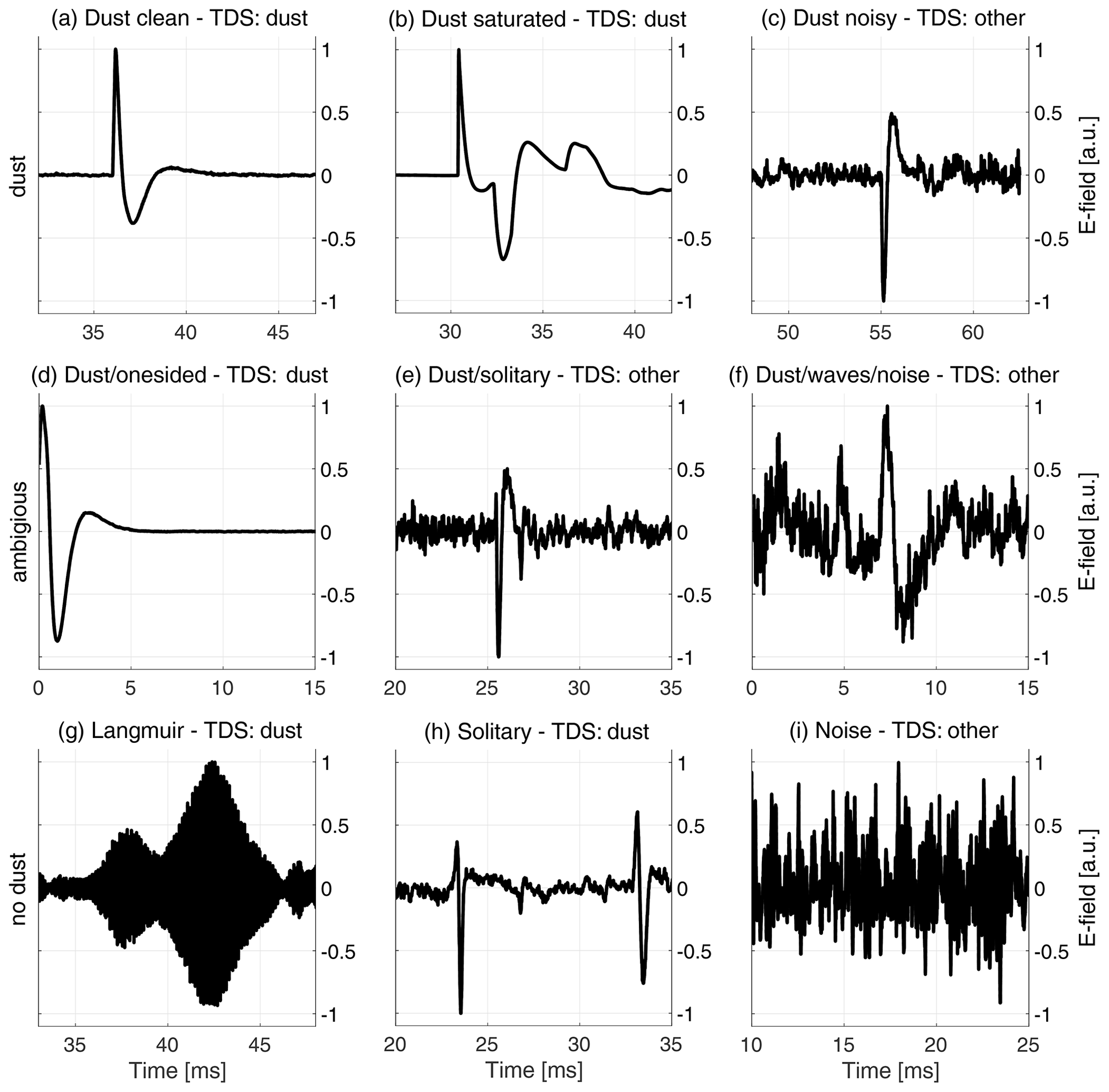
Figure 1 Waveforms recorded by the TDS receiver and measured by one of the RPW antennas. The signal label, classified by the TDS classification algorithm, is included for each snapshot in the subplot titles. The top row presents dust waveforms: (a) is a clean dust impact waveform; (b) shows a dust impact that saturates the receiver unit (or reaches the non-linearity limit); and (c) presents a weak dust impact signal that is strongly affected by noise. The middle row presents ambiguous waveforms: (d) might be a dust impact, but information is limited by the signal framing; (e) is likely a dust impact, but the signal shape resembles solitary waves and is strongly affected by noise; and (f) might be a dust impact, but noise and possible electromagnetic waves make the signal difficult to interpret. The bottom row presents waveforms without dust: (g) shows Langmuir waves, characterized by the high-frequency E-field oscillations with a lower-frequency amplitude modulation; (h) presents solitary waves, which sometimes resemble dust impact waveforms; and (i) shows a signal dominated by noise, without any clear features. Note that the full (63 ms) snapshots are zoomed to 15 ms intervals around the interesting features and that the signal amplitudes are normalized to ± 1 and centered around zero for illustrative purposes.

2 Observations and data acquisition

2.1 The Radio and Plasma Waves (RPW) Instrument and the Time Domain Sampler (TDS) receiver

This work focuses on electric field signals (i.e., waveforms) observed by the Radio and Plasma Waves (RPW) instrument on board the Solar Orbiter (Maksimovic et al., 2020). The RPW instrument consists of three antennas operating synchronously and the measured electric potential is recorded by the Time Domain Sampler (TDS) receiver unit (Soucek et al., 2021).

The TDS receiver is designed to capture plasma waves (such as ion acoustic and Langmuir waves) in the frequency range 200 Hz–100 kHz, in addition to the dust impact signals (Soucek et al., 2021). The antenna voltages are converted to electric field values using the antenna effective lengths but are otherwise uncalibrated. We consider only signals sampled with a sampling rate of 262.1 kHz in snapshots of 16 384 time steps, acquired when the TDS receiver was operating in the XLD1 mode.

The XLD1 mode is the most commonly used observational mode of the RPW–TDS system (Soucek et al., 2021). XLD1 is a hybrid mode, where channel 3 (CH₃) is operating in monopole mode, while channel 1 (CH₁) and channel 2 (CH₂) are operating in dipole mode:

$$\begin{array}{}\text{(1)}& {\displaystyle }\mathit{C}{\mathit{H}}_{\mathrm{1}}=\left({\displaystyle \frac{V_{\mathrm{1}}-V_{\mathrm{SC}}}{L_{\mathrm{1}}}}\right){\widehat{\mathit{L}}}_{\mathrm{1}}-\left({\displaystyle \frac{V_{\mathrm{3}}-V_{\mathrm{SC}}}{L_{\mathrm{3}}}}\right){\widehat{\mathit{L}}}_{\mathrm{3}}\text{(2)}& {\displaystyle }\mathit{C}{\mathit{H}}_{\mathrm{2}}=\left({\displaystyle \frac{V_{\mathrm{2}}-V_{\mathrm{SC}}}{L_{\mathrm{2}}}}\right){\widehat{\mathit{L}}}_{\mathrm{2}}-\left({\displaystyle \frac{V_{\mathrm{1}}-V_{\mathrm{SC}}}{L_{\mathrm{1}}}}\right){\widehat{\mathit{L}}}_{\mathrm{1}}\text{(3)}& {\displaystyle }\mathit{C}{\mathit{H}}_{\mathrm{3}}=\left({\displaystyle \frac{V_{\mathrm{2}}-V_{\mathrm{SC}}}{L_{\mathrm{2}}}}\right){\widehat{\mathit{L}}}_{\mathrm{2}},\end{array}$$

where V_i−V_SC denotes the potential difference between antenna i and the spacecraft body along the antenna boom with unit vector ${\widehat{\mathit{L}}}_i$ and effective length L_i. For this work however, the three RPW antenna signals are all converted to monopole electric field signals (E₁, E₂, E₃) by the following conversion:

$$\begin{array}{}\text{(4)}& {\displaystyle }\begin{array}{rl}{\mathit{E}}_{\mathrm{1}}& =\mathit{C}{\mathit{H}}_{\mathrm{3}}-\mathit{C}{\mathit{H}}_{\mathrm{2}}=\left({\displaystyle \frac{V_{\mathrm{2}}-V_{\mathrm{SC}}}{L_{\mathrm{2}}}}\right){\widehat{\mathit{L}}}_{\mathrm{2}}\\ & -(\left({\displaystyle \frac{V_{\mathrm{2}}-V_{\mathrm{SC}}}{L_{\mathrm{2}}}}\right){\widehat{\mathit{L}}}_{\mathrm{2}}-\left({\displaystyle \frac{V_{\mathrm{1}}-V_{\mathrm{SC}}}{L_{\mathrm{1}}}}\right){\widehat{\mathit{L}}}_{\mathrm{1}})\\ & =\left({\displaystyle \frac{V_{\mathrm{1}}-V_{\mathrm{SC}}}{L_{\mathrm{1}}}}\right){\widehat{\mathit{L}}}_{\mathrm{1}}\end{array}\text{(5)}& {\displaystyle }{\mathit{E}}_{\mathrm{2}}=\mathit{C}{\mathit{H}}_{\mathrm{3}}=\left({\displaystyle \frac{V_{\mathrm{2}}-V_{\mathrm{SC}}}{L_{\mathrm{2}}}}\right){\widehat{\mathit{L}}}_{\mathrm{2}}\text{(6)}& {\displaystyle }\begin{array}{rl}{\mathit{E}}_{\mathrm{3}}& =\mathit{C}{\mathit{H}}_{\mathrm{3}}-\mathit{C}{\mathit{H}}_{\mathrm{2}}-\mathit{C}{\mathit{H}}_{\mathrm{1}}={\mathit{E}}_{\mathrm{1}}-\mathit{C}{\mathit{H}}_{\mathrm{1}}\\ & =\left({\displaystyle \frac{V_{\mathrm{1}}-V_{\mathrm{SC}}}{L_{\mathrm{1}}}}\right){\widehat{\mathit{L}}}_{\mathrm{1}}-(\left({\displaystyle \frac{V_{\mathrm{1}}-V_{\mathrm{SC}}}{L_{\mathrm{1}}}}\right){\widehat{\mathit{L}}}_{\mathrm{1}}\\ & -\left({\displaystyle \frac{V_{\mathrm{3}}-V_{\mathrm{SC}}}{L_{\mathrm{3}}}}\right){\widehat{\mathit{L}}}_{\mathrm{3}})=\left({\displaystyle \frac{V_{\mathrm{3}}-V_{\mathrm{SC}}}{L_{\mathrm{3}}}}\right){\widehat{\mathit{L}}}_{\mathrm{3}}.\end{array}\end{array}$$

The Solar Orbiter RPW–TDS detection threshold is ∼ 5 mV, allowing dust impact identification of the cosmic dust flux with typical diameters ranging from ∼ 100 to ∼ 500 nm (Zaslavsky et al., 2021).

2.2 The Triggered Snapshot WaveForms (TSWF) data product and the TDS classifier

For this project, we use the Triggered Snapshot WaveForms (TSWF) data product, processed with software version 2.1.1 and acquired over a 25-month period, spanning between 15 June 2020 to 14 July 2022. The TSWF data product consists of signal packets (63 ms snapshots) that are down-linked only if the classification algorithm on board the Solar Orbiter is triggered. The accuracy of the on-board classification algorithm is therefore important in order to optimize the data transfer and provide reliable data products for statistical analysis.

The input to the on-board classification algorithm, hereafter named the TDS classifier or the TDS classification algorithm, is the 63 ms signal packet, while the output is categorized into one out of three labels: dust, wave or other. Figure 1 presents a few examples of recorded snapshots with included labels, as classified by the TDS classification algorithm. The TDS classifier assigns the label based on three extracted features as follows:

1. The snapshot peak amplitude (V_max)

2. The ratio of the peak amplitude to the median absolute value of the signal ($V_{\max }/V_{\mathrm{med}}$)

3. The full width half maximum (BW) of the main spectral peak, identified by analyzing the discrete Fourier transform of the signal.

The signal label is then determined by comparing the extracted feature values against configurable thresholds. The threshold criterion reflects that observations of waves are typically narrow band (low BW) and the peak of the signal is not much larger than the median value (low $V_{\max }/V_{\mathrm{med}}$). In contrast, dust observations are sharp non-periodic signals (high BW) that generally have a high maximum to median amplitude ratio (high $V_{\max }/V_{\mathrm{med}}$). For more detailed descriptions of the TDS classifier, see Soucek et al. (2021).

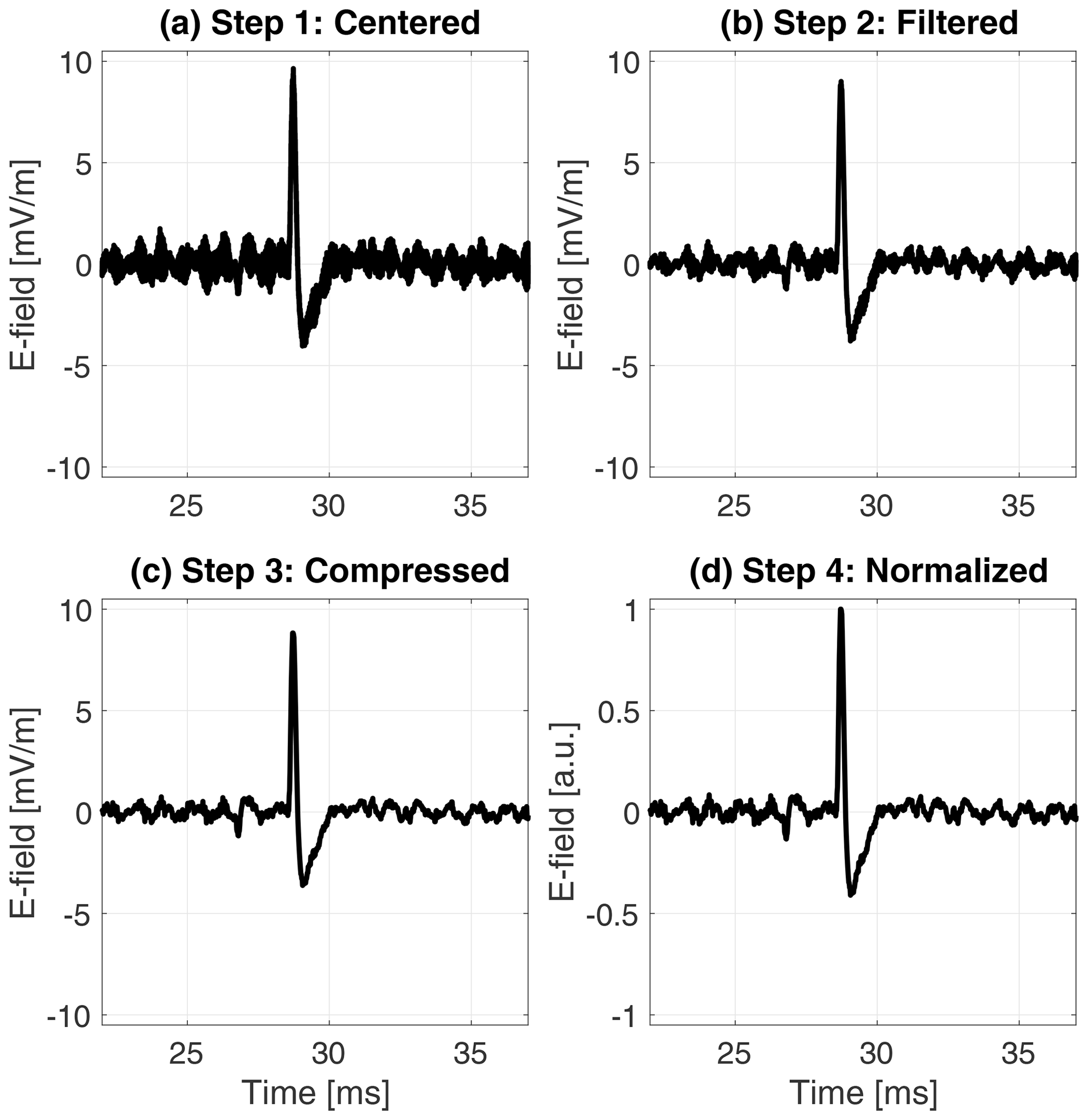
Figure 2 A dust waveform observed by antenna 2 on 8 September 2021. The panels illustrate the different stages of the pre-processing procedure. (a) The electric field offset is removed and the signal is centered around 0 mV m⁻¹. (b) The signal is filtered by a median filter over seven time steps to reduce the high-frequency noise. (c) The signal is compressed by a factor of 4 to reduce the data size. (d) The waveform is normalized by the maximum absolute value of the signal in order to ease the parameter optimization of the machine learning classifier. Note the waveform is zoomed to a 15 ms time period around the dust impact in order to better visualize the impact shape modification by the pre-processing procedure.

Figure 3 Data flow, from the TDS data sets to the machine learning performance metrics. The diagram illustrates the data flow by the black arrows and the applied process by the arrow label. The cylinders indicate the signal waveforms and the cylinder color indicates the associated label. The gray circles mark data transformation processes. The random draw of the TDS data and the pre-processing is explained in Sect. 3.1, while the manual labeling is described in Sect. 3.2. A description of the randomization and splitting of the manually labeled data into a training and a testing set is included in Sect. 3.3. Sections 3.4 and 3.5 explain the training and testing of the machine learning classifiers. Finally, the performances of the machine learning classifiers are compared and evaluated in Sect. 4.1.

Figure 1 illustrates that it is challenging to detect and separate dust signals from the plural of other signal shapes. In particular, the dust waveform in panel (c) is classified as other, while the Langmuir wave and solitary wave snapshots in panels (g) and (h) are erroneously classified as dust by the TDS classification algorithm. For more information on observations of Langmuir and ion acoustic waves in the Solar Orbiter data, see e.g., Soucek et al. (2021), and for an analysis of Wind observations of electrostatic solitary waves, see Malaspina et al. (2013).

3 Machine learning-based framework for automatic dust impact detection

The goal of the machine learning classifier is to take a monopole RPW snapshot as an input and automatically output if the signal contains a dust impact or not. For this purpose, we use a supervised classifier. A supervised classifier relies on manually labeled data to learn (i.e., train) the function that maps the input observation (the electric field signal) to the output label. For this work, we focus exclusively on detecting dust impact signals, we therefore use the binary labels: dust or no dust. Additional labels, such as: ion-acoustic waves, Langmuir waves and solitary waves, could however be implemented in a similar machine learning-based framework.

3.1 Data pre-processing for machine learning classification

In order to construct a balanced data set, we selected ∼ 1500 waveforms classified as dust and ∼ 1500 waveforms classified as wave/other by the TDS classification algorithm. The signals were randomly drawn from the TDS data archive and acquired between 15 June 2020 to 16 December 2021. The TDS signals were then pre-processed to standardize the input to the classifier and speed up the training. Standardized data further reduces bias effects and makes the manual labeling of the signals easier to conduct. For this work, a four-step pre-processing procedure was used independently on each antenna signal, the pre-processing procedure applied on a sample signal is illustrated in Fig. 2.

1. Remove the signal offset. The electric field offset is removed by subtracting the raw signal with the median of a heavily filtered version of the raw data. A sliding median filter over 21 time steps was selected by visual inspection of the noise characteristics. The removal of the electric field offset centers the signal around zero and reduces bias effects from offset waveforms.

2. Filter the data. The signal is filtered using a sliding median filter over seven time steps in order to reduce the high-frequency noise. The seven time-step filter was selected by inspecting the power spectrum of impact signals and by noticing that most information above (f_N=35 kHz) is buried in noise, although the TDS sampling frequency is higher (f_s=262.1 kHz), thus making a filter length ($<f_{\mathrm{s}}/f_{\mathrm{N}}\approx \mathrm{7.5}$) appropriate without significant loss of information.

3. Compress the data. The signal is re-sampled with a compression factor of 4 using linear 1-dimensional interpolation. The compression is done to speed up the training of the classifier, resulting in a re-sampling from 16 384 to 4096 time steps.

4. Normalize the signal. The data are normalized to be between −1 and 1 by dividing all data samples with the maximum absolute value of the signal. The normalization makes the machine learning classifier more robust to variations in the signal strength and eases the parameter optimization during training.

3.2 Manual waveform labeling

Manually labeled data are used both to train the machine learning classifiers and to test the performance of the trained models. Thus, great care is needed in order to construct a high-quality labeled data set, without significant contamination of corrupted data files, biases and mislabeled signals.

We manually labeled the data into either dust or no dust. Each signal was displayed without indications of the previously assigned label by the TDS classifier in order to reduce bias effects. Furthermore, a zoom function was used to investigate the areas of interest, and options were included both to correct labeling mistakes by the user and to indicate ambiguous signals that do not clearly fit into any label (dust or no dust). Appendix A presents the graphical user interface (GUI) that was used to label the 3000 observations.

It should be noted that 134 signals (i.e., 4.5 %), out of 3000 manually labeled waveforms, were marked as ambiguous and did not clearly fit into either the dust or no dust label, see the middle row of Fig. 1 for ambiguous examples. Furthermore, the manual waveform labeling was done by one scientist, although with consultations with other experts. Thus, it is to be expected that different scientists will disagree on a proportion (up to 5 %) of the manual labels. The disagreement level could possibly be reduced if several experts labeled the same data set, and the labeling consensus was used as the effective waveform label.

3.3 Developing the machine learning classifiers

The manually labeled data were split into a training set (containing 80 % of the data) and a testing set (with the remaining 20 %). The training data are used to optimize the free parameters of the machine learning classifiers with respect to the assigned labels, while the testing data are used as an independent set to evaluate the performance of the trained classifiers. The performance of a machine learning classifier is quantified by comparing the outputs of the trained model to the labels of the testing data. Figure 3 illustrates the data flow, from the TDS data sets to the machine learning performance metrics.

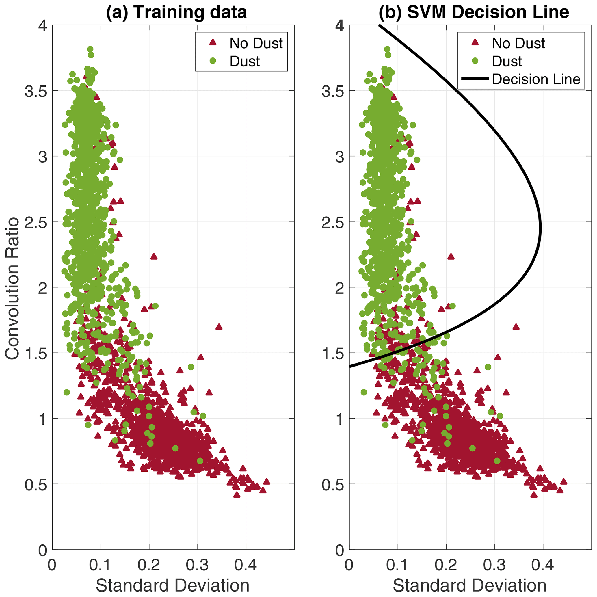
Figure 4 (a) The (1×2) feature vectors extracted from all (2400) observations in the training data, the associated labels are indicated in green (dust) and red (no dust). (b) The SVM decision line is defined as a second-order polynomial, obtained by minimizing the non-separable SVM cost function. The optimized SVM decision line appears to be reasonable, and most observations are separable in the training data.

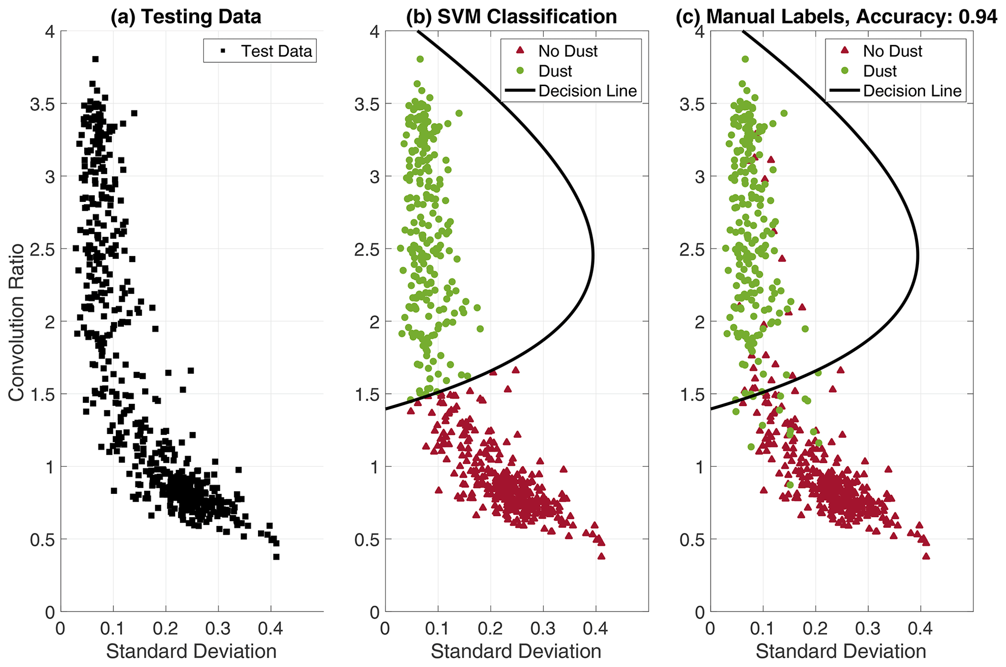
Figure 5 (a) The (1×2) feature vectors extracted from the testing data (600 observations with hidden labels). (b) The testing data are classified using the trained SVM decision line, where all observations within the polynomial line are classified as dust, while all observations outside are classified as no dust. (c) The “true” labels (from the manual labeling) are revealed. It is clear that some observations are confused, predominantly near the decision line. Still, the SVM classifier achieves an overall classification accuracy of 94 %, calculated by comparing the outputs from the SVM classification (b) to the “true” labels (c).

There are numerous machine learning techniques that are suitable for time series classification. In this work, we focus on two well-known techniques: the support vector machine (SVM), described in Sect. 3.4, and the convolutional neural network (CNN), discussed in Sect. 3.5.

3.4 The support vector machine (SVM)

The support vector machine (Boser et al., 1992; Cortes and Vapnik, 1995) is a robust and versatile classification algorithm, considered to be one of the most influential approaches in supervised learning (Goodfellow et al., 2016). SVMs learn the decision hyperplane that maximizes the discriminative power between the observations categorized into two classes (in this case, dust or no dust). However, SVMs are highly dependent on the representation of the data and often achieve sub-optimal performance on high-dimensional data (when used directly). In this case, the observations from three antenna measurements, each with 4096 time steps, are both high-dimensional and noisy (each time step contains little information). It is therefore common to extract important characteristics (i.e., features) from the data to provide the SVM with compactly represented information with less noise and redundancies.

3.4.1 Feature extraction

In order to develop a baseline machine learning classifier, comparable to the on-board TDS classification algorithm, a simple 2-dimensional SVM classifier was considered. Thus, every observation with dimension (3×4096) is represented by a 2-dimensional feature vector (1×2). After some initial testing, we selected two features that had a high discriminative power between the dust and no dust observations.

1. The standard deviation. The mean standard deviation is calculated over the three antenna channels, each with 4096 time steps. The standard deviation is an appropriate feature since normalized dust signals typically have a lower mean standard deviation than normalized no dust signals.

2. The convolution ratio. The log ₁₀ value of the convolution ratio ($|\mathrm{conv}{|}_{max}/|\mathrm{conv}{|}_{\mathrm{median}}$) is calculated, where $\left|\mathrm{conv}\right|$ is the absolute values of the convolution of the antenna signals with a normalized Gaussian of width 0.5 ms. $|\mathrm{conv}{|}_{max}$ is the maximum value of $\left|\mathrm{conv}\right|$, while $|\mathrm{conv}{|}_{\mathrm{median}}$ is the median. The convolution ratio was selected as a feature since the dust signals typically have a larger convolution ratio than the no dust signals. The Gaussian width of 0.5 ms was experimentally found to give high correlations with dust impact signals.

3.4.2 Training the support vector machine

The two features (standard deviation and convolution ratio) were extracted from all observations in the training data. The decision hyperplane, in this 2-dimensional case a decision line, is defined by a polynomial of degree 2 that is optimized by minimizing the non-separable SVM cost function, see e.g., Theodoridis and Koutroumbas (2009) for details. The SVM classifier was trained with a slack variable factor of 1 and equal weighting between the dust and no dust observations. The 2-dimensional SVM is computationally inexpensive to optimize with a training time of ∼ 1 s on a modern laptop. Figure 4 illustrates the training of the SVM classifier.

Figure 6 The signal examples are presented in (a)–(i), the manual labels are indicated along the y axis and the predicted labels, classified by the SVM decision line, are presented in the subplot titles. Panel (j) presents the associated signal examples in the 2-D feature vector space along with the SVM decision line. The dust signals are illustrated in green, the ambiguous signals are marked in yellow and the no dust signals are indicated in red. The SVM classifier provides mostly explainable outputs. The clear dust signals (a–b) are located well within the SVM decision line, the ambiguous signals (e–f) are located near the decision line, while the no dust signals (g–i) are clearly located outside. However, dust signal (c) is erroneously located just outside the decision line, this can possibly be explained by the weak signal-to-noise ratio. In addition, signal (d) is located well within the decision line, although this signal is labeled ambiguous-no dust due to the signal framing, this indicates that the SVM might have difficulties classifying signatures located at the edge of the snapshot frame. Note that the signals are zoomed to 15 ms intervals around the interesting features, similar to the examples in Fig. 1.

3.4.3 Testing the support vector machine

The performance of the trained SVM classifier is evaluated using the independent testing data, i.e., the remaining manually labeled data (20 %) that were not used for training the classifier. Figure 5 presents the SVM classification performance on the testing data.

Overall, the SVM classifier achieves a classification accuracy of 94 % on the testing data using the 2-dimensional feature vectors. Note that the inclusion of additional extracted features can possibly enhance the SVM performance. Several additional features can be considered, such as the mean amplitude of the signal, the range between the signal maximum and minimum values and the cross-correlation length (the time lag to the first zero crossing).

3.4.4 Explainability of the support vector machine

Ideally, we want to develop a machine learning classifier that not only has a high accuracy, but also makes decisions that are understandable for human experts (Holzinger et al., 2019). In other words, we want to be able to explain why the machine learning classifier selected the predicted class for a given observation. In machine learning, this is often referred to as the explainability of the trained classifier. Figure 5 presents the testing data in the 2-D feature vector space, but this plot gives no clear indications of how different signal shapes are distributed and which signatures are confused by the SVM classifier. In order to better understand the decisions made by the SVM classifier, the signal examples in Fig. 1 are studied in detail. The analysis is presented in Fig. 6.

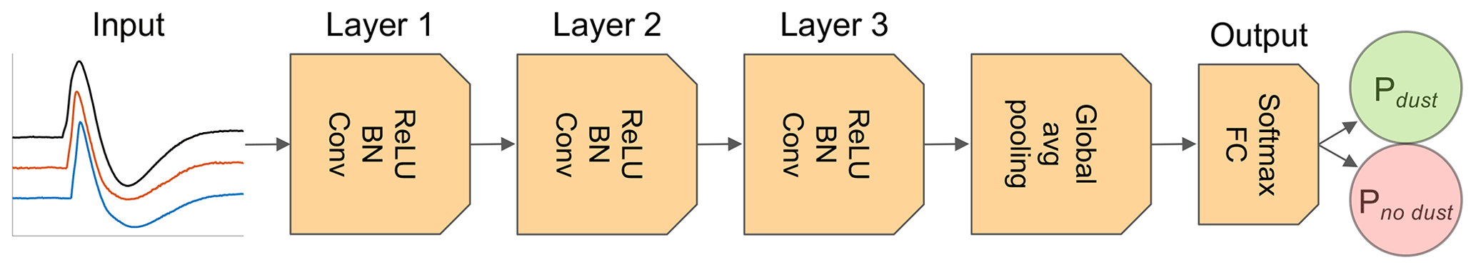
Figure 7 The three-layer fully convolutional network used for the dust impact classification task. The input to the network is the (3×4096) waveform. The feature extraction process is defined by three convolutional layers, consisting of 128, 256 and 128 independent filters with kernel lengths of 8, 5 and 3 weights, respectively. Batch normalization (BN) is used at each convolutional layer to regularize the inputs and the rectified linear unit (ReLU) function was used as the activation function. Finally, the output of the convolutional layers (with dimension 128×4096) is averaged in the global pooling layer to a feature vector with dimension (128×1). The class score is then determined in a fully connected (FC) network layer and the output label probabilities (P_dust, P_no dust) are calculated using the softmax function. The figure is adopted from Wickstrøm et al. (2021).

It should be noted that the signal examples in Fig. 6 are not representative for the general distribution of observations in the 2-D feature vector space, since most observations are clustered in distinct dust and no dust regions, as can be seen in Fig. 5. Figure 6 focuses mostly on signal examples that are challenging to classify. Still, Fig. 6 indicates that the SVM classifier provides mostly comprehensible outputs, but might have difficulties classifying weak dust impact signals and signals with important signatures located at the edge of the snapshot frame.

3.5 The convolutional neural network (CNN)

Convolutional neural networks are algorithms designed for processing grid-like data and have achieved premium performance on a number of different tasks in the recent decade, such as image (He et al., 2016; Kvammen et al., 2020), video (Karpathy et al., 2014) and time series (Wang et al., 2017; Wickstrøm et al., 2021) classification.

3.5.1 Feature extraction

Unlike the SVM, the CNN does not require pre-defined feature extraction routines. Instead, the CNN extracts the features based on a chain of convolution operations and automatically optimizes the convolution filters based on the training data and the associated labels.

For this work, we employed the three-layer fully convolutional network architecture presented in Wang et al. (2017) and suggested for time series classification after extensive testing (Wickstrøm et al., 2022; Fawaz et al., 2020; Karim et al., 2019). The rectified linear unit (ReLU) function (Glorot et al., 2011) was used as the activation function and Batch Normalization (BN) (Ioffe and Szegedy, 2015) was used at each convolutional layer in order to regularize the network and accelerate the training process. Figure 7 presents the employed CNN architecture.

Figure 8 (a) The testing data (600 observations with hidden labels) are visualized by a dimension-reduced t-SNE map, where similar feature vectors are modeled by nearby points, while dissimilar observations are modeled by distant points with high probability. (b) The testing data classified by the trained CNN. (c) The “true” manual labels are presented. Only a few observations, predominantly in the transition region between the dust and no dust observations, are confused. An overall classification accuracy of 96 % is calculated by comparing the labels predicted by the CNN to the manual labels. Note that the presented testing data is the same data set that was used to test the SVM classifier, illustrated in Fig. 5.

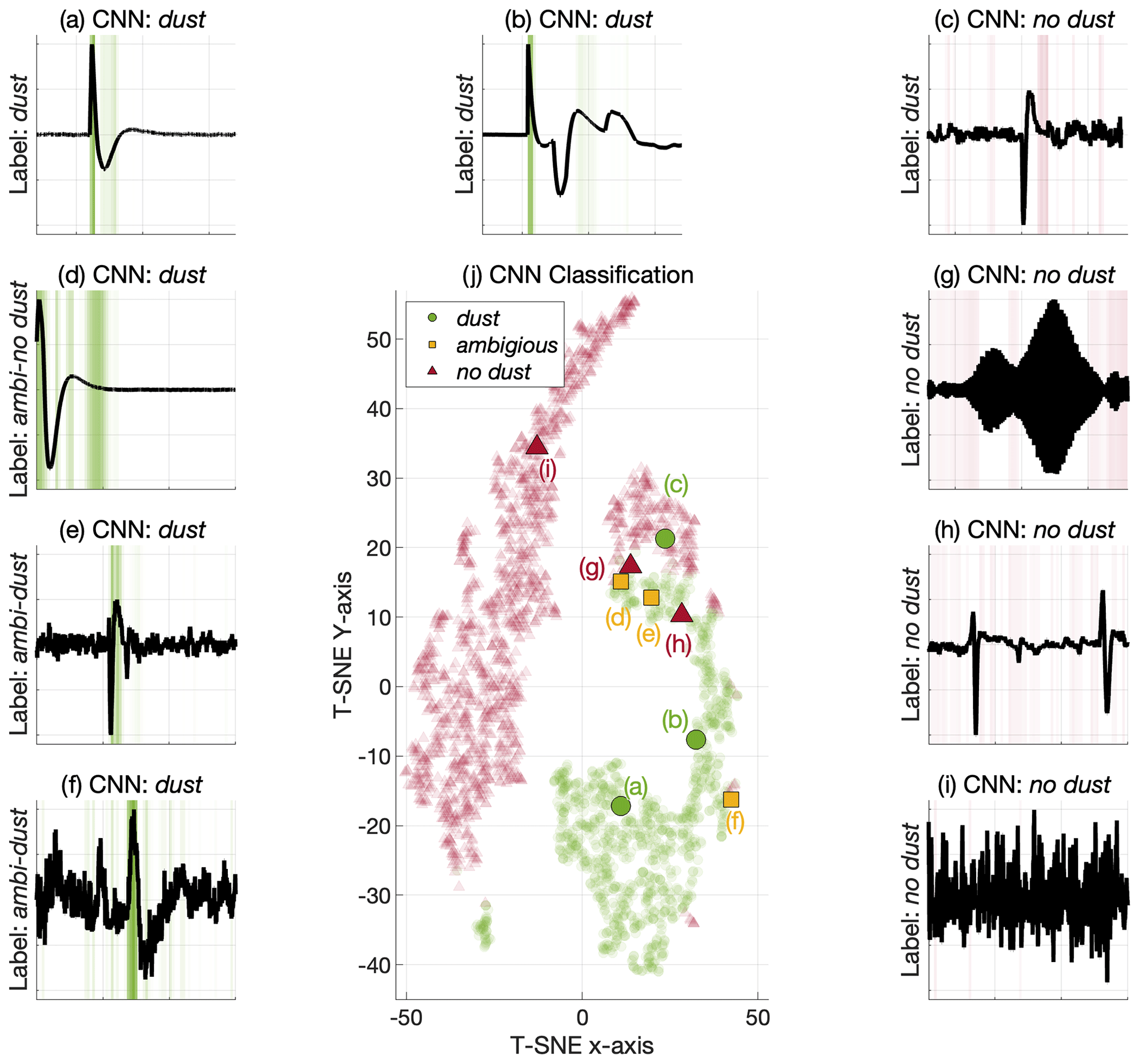
Figure 9 The signal examples and the CAM analysis are presented in (a)–(i), the manual labels are indicated along the y axis and the predicted label, classified by the CNN, is presented in the subplot titles. The highlighted green color indicates the CAM values associated with the dust class, the green regions therefore emphasize the regions that are considered important by the CNN for detecting dust impact signatures. Similarly, the red color indicates the regions that are influential for the no dust class. Note that the signals are zoomed to 15 ms intervals around the interesting features, similar to Figs. 1 and 6. Panel (j) presents the associated signal examples in the t-SNE space along with the training data signals as transparent points. The dust signals are illustrated by the green dots, the ambiguous signal examples are marked in yellow and the no dust signals are indicated in red. The t-SNE map shows that the clear dust signals (a–b) are distinctly located in a green (dust) region, whereas the clear no dust signal (i) is distinctly located in a red (no dust) region. The remaining signals are located in more mixed regions. It should however be noted that the observations are represented by a 128-dimensional feature vector in the CNN and that the (2-D) t-SNE representation presented in (j) diminishes a lot of information, meaning that even the signals located in a mixed region of the t-SNE plot might be separable in the 128-dimensional feature vector space.

3.5.2 Training the convolutional neural network

The three-layer fully convolutional network consists of 267 010 free parameters (weights and biases) that need to be optimized to solve the dust impact classification task. The free parameters are randomly initialized and thereafter optimized using the ADAM gradient descent optimizer (Kingma and Ba, 2014). The CNN was trained for 225 epochs with a cross-entropy loss function using the 2400 labeled observations in the training data. CNNs are computationally expensive to optimize, as compared to the SVM classifier, and a training time of ∼ 20 min was required using TensorFlow on a MacBook Pro with a 32-core M1 Max GPU chip. For more details on neural network training and optimization, see for example (Montavon et al., 2012).

3.5.3 Testing the convolutional neural network

In order to visualize the features extracted by the CNN, we employ the t-distributed Stochastic Neighbor Embedding (t-SNE) method (Van der Maaten and Hinton, 2008). The t-SNE method is used for visualizing high-dimensional data by assigning each observation a location in a 2-D space such that similar observations are modeled by nearby points, while dissimilar observations are modeled by distant points with high probability. The (128×1) testing feature vectors, extracted in the global pooling layer, are presented in a 2-D t-SNE map in Fig. 8, along with a visualization of the CNN classification performance.

Overall, the CNN obtains a high (≳ 95 %) classification accuracy and might therefore be suitable for automatic processing of electric field signals observed by the RPW instrument on board the Solar Orbiter.

3.5.4 Explainability of the convolutional neural network

Neural networks have traditionally been regarded as black boxes (Shwartz-Ziv and Tishby, 2017; Alain and Bengio, 2016), where the network carries out the desired task, but the network decisions are difficult to interpret. However, progress has been made in recent years for making the neural network decisions more accessible and easier to interpret (i.e., explainable) for human users (Samek et al., 2021). In this section, we analyze the CNN decisions by employing class activation maps and the previously described t-SNE method.

Class activation maps (CAMs) (Zhou et al., 2016) highlight the regions of the data that are important for a considered label (l) by analyzing the features extracted in the global pooling layer and the weights in the FC layer that are associated with label (l), see e.g., (Wang et al., 2017) for a detailed description. The outcome of the CAM analysis is that we can visualize the sections of the signal that are influential for the CNN classification decision. Figure 9 presents the CAM analysis of the signal examples in Fig. 1 along with an illustration of the signal features in a dimension-reduced t-SNE space. Note that the t-SNE mapping in Fig. 9 is different from the t-SNE mapping in Fig. 8, since Fig. 9 considers a different CNN where the signal examples are specifically excluded from the training data.

Table 1 The TDS, SVM and CNN classification performance metrics: accuracy, precision, recall and F1-score. The SVM and CNN scores and error values are the mean and the standard deviation across 10 training runs. The bold numbers indicate statistically enhanced performance with a significance level of 0.01, computed using a t-test.

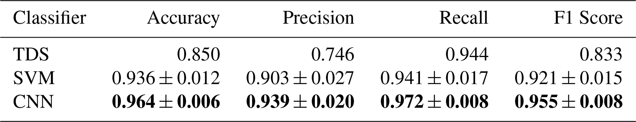
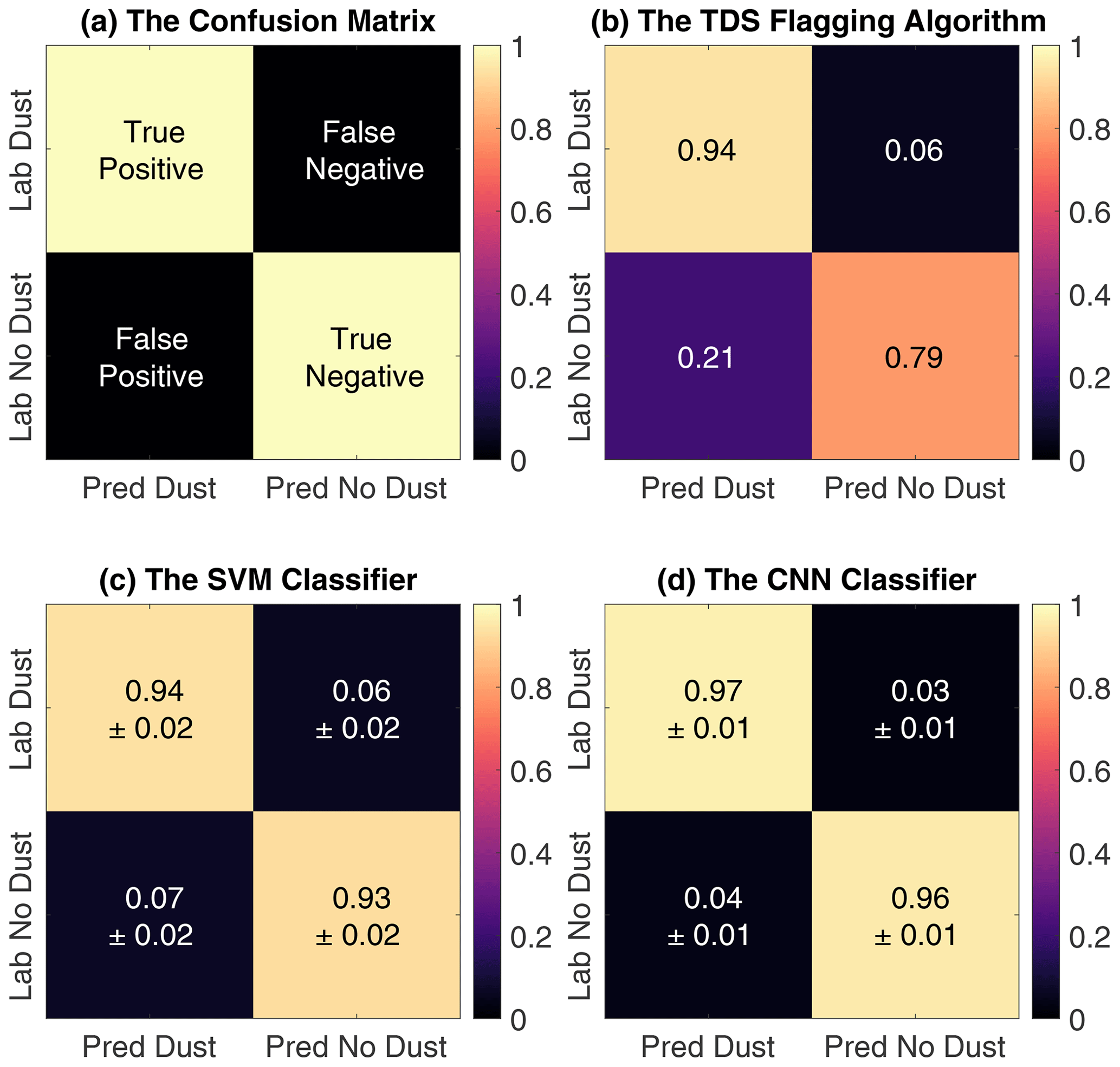
Figure 10 (a) The confusion matrix entries are described by the true (correctly classified) and false (erroneously classified) values; compared to the manual labels (Lab), positive indicates dust predictions (Pred), and negative indicates no dust predictions. (b) The TDS classifier confuses dust and no dust observations, where a significant proportion (>0.20) of dust predictions are manually labeled as no dust. (c) The SVM classifier predicts both dust and no dust observations with a high (>0.90) accuracy. (d) The CNN classifier predicts a very large (>0.95) proportion of both dust and no dust observations correctly.

The CAM analysis in Fig. 9 illustrates that the CNN makes classification decisions that are comprehensible (in most cases). It is however interesting to note that signal (c), manually labeled as dust, is erroneously classified as no dust by the CNN, and that this decision is largely based on the tail (the relaxation period) of the impact signal. It should however be noted that it is more difficult to explain the no dust predictions than the dust predictions, since the no dust CNN decisions are based on the lack of a signature (dust impact) rather than on the presence of a signature. In addition, signal (d), manually labeled as ambiguous-no dust, is classified as dust by the CNN, and this decision is based on a wide region of the signal with emphasis on the tail of the (ambiguous) dust impact signal, this section might not have been highlighted as particularly important by a human expert.

In general however, the CNN achieves a high accuracy (≳ 95 %) and makes decisions that are mostly in line with human interpretation. It is therefore reasonable to infer that the CNN will have a performance comparable to the agreement level between human experts, where disagreement predominantly occurs for ambiguous and noisy signals, while clear dust and clear no dust signals are classified correctly.

4 Results and discussions

4.1 Analysis of the classification performance

The average classification performance is obtained by training and testing the machine learning classifiers over 10 runs, each run with different training and testing sets. The classifiers are initialized from scratch and the training and testing sets are selected independently 10 times by randomization and splitting of the manually labeled data, as indicated by the gray circles in Fig. 3. The average class-wise performance of the on-board TDS classifier and the machine learning SVM and CNN classifiers are summarized as confusion matrices in Fig. 10. Overall, the CNN has the highest performance for both dust and no dust classification. In addition, both the SVM and the CNN classifiers obtain stable performances with only small variations for each run.

The classification performance is further evaluated by the accuracy, precision, recall and F1 score. The definitions for the performance metrics are included in Appendix B. The average performance metrics, calculated over 10 runs, are summarized in Table 1. Again, the CNN has the highest performance across all metrics. The CNN obtains a significant improvement in the classification performance with a statistical significance at a level of 0.01, computed using a t-test. The t-test was computed in a pairwise manner between both the CNN and the SVM scores and the CNN and the TDS scores. In all cases, the enhanced performance of the CNN classifier was significant.

The results from both the confusion matrices and the performance metrics strongly suggest that the SVM and CNN classifiers provide binary classification results with higher reliability than the TDS classifier and further that the CNN is the most reliable classifier overall. We therefore propose that the CNN classifier (or similar tools) should be considered for post-processing of the TDS data product in statistical studies of dust impacts observed by the Solar Orbiter RPW instrument.

In addition, it should be noted that 134 signals (i.e., 4.5 %), out of 3000 manually labeled waveforms, were marked as ambiguous, illustrated by the yellow cylinder in Fig. 3, and did not clearly fit into either the dust or no dust label, see Fig. 1 for label examples. It is therefore improbable to achieve a classification accuracy exceeding ∼ 98 % for the considered data set, and an accuracy approaching ∼ 99 % should be considered suspicious and can be an indication of over-fitting.

Both the trained SVM and CNN classifiers are computationally inexpensive to run. One thousand observations are classified in 5 s using the SVM model, while the CNN classifier requires 50 s on a modern laptop, including the needed time for pre-processing and feature extraction. The proposed machine learning classifiers are therefore suitable for processing large data sets with thousands of new observations acquired every month as the Solar Orbiter continues its operation.

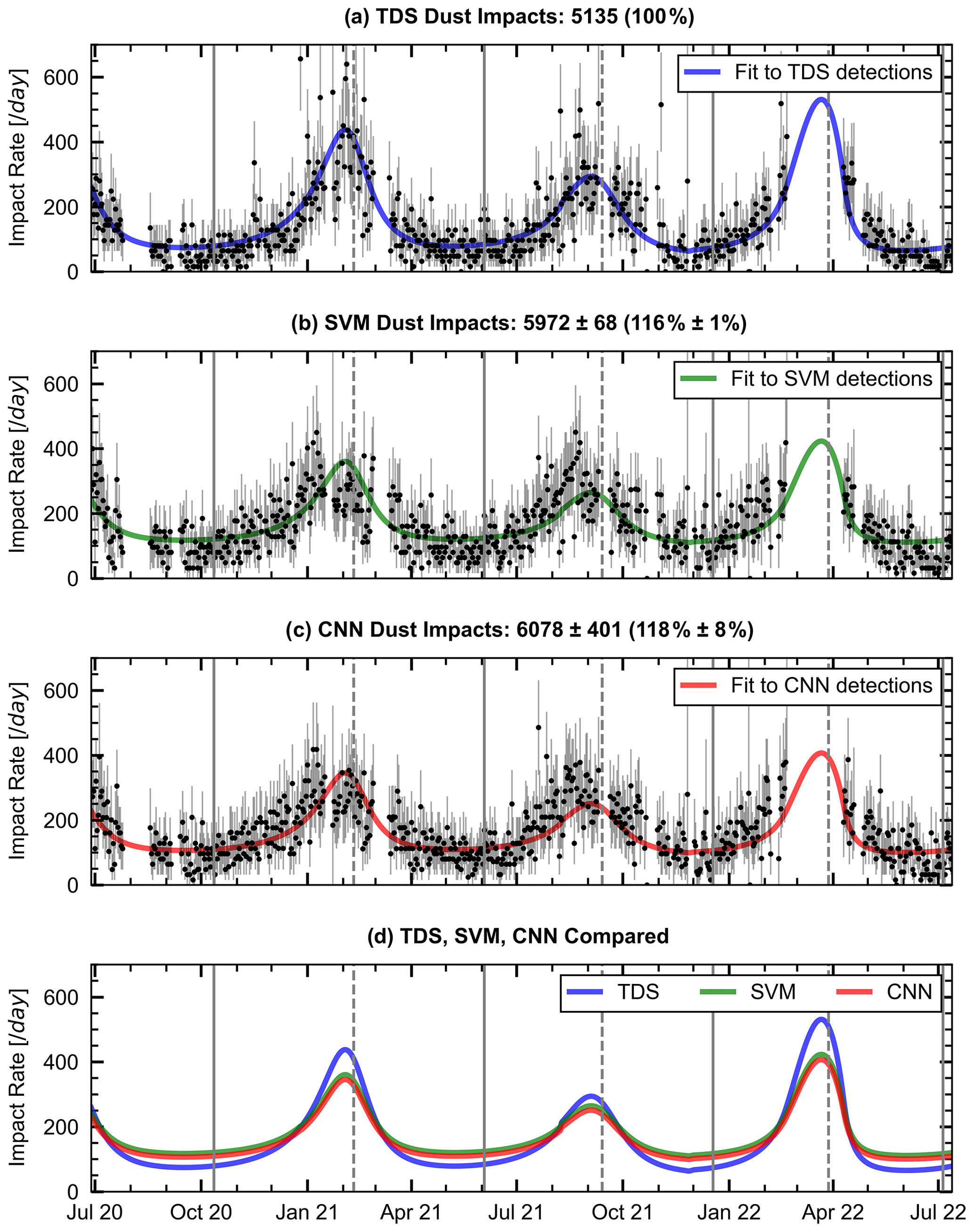
Figure 11 (a) The daily dust impact rates according to the TDS classifier. The full vertical lines indicate times when the Solar Orbiter is at aphelion, while the dashed lines indicate times at perihelion. (b) The median of the daily impact rates classified by 10 trained SVM classifiers. (c) The median of the daily impact rates from the 10 CNN classifiers. The impact rate function curves are obtained by fitting the dust flux model from Zaslavsky et al. (2021), Eq. (7). (d) The impact rate function cures are compared. The SVM and CNN dust impact rates are very similar, whereas the TDS provides notably smaller impact rates at aphelion and higher impact rates at perihelion. The accumulated dust impact detections for the TDS classification algorithm and the mean and standard deviation of the dust impact detections for the 10 CNN and SVM classifiers are presented in the subplot titles. Note that the large data gap around April 2022 (perihelion 3) is due to a different observational setup for the Solar Orbiter RPW–TDS system, where the sampling frequency was doubled. These data were excluded since it can not be reliably classified by the SVM/CNN methods without additional data processing and/or training.

4.2 The dust impact rate

In this section, we use the trained classifiers to automatically process a large data set, consisting of 104 032 observations. This data set contains all TSWF observations acquired over a 25-month period, spanning between 15 June 2020 to 14 July 2022, that satisfy the criteria in Sect. 2.1 (sampling rate of 262.1 kHz, 16 384 time steps and XLD1 mode).

Figure 11 presents the TDS, SVM and CNN daily impact rates with included error estimates. The daily impact rate is calculated from the automatically detected daily dust impact number and the time-dependent TDS–RPW duty cycle. The number of dust particles detected by the Solar Orbiter on each day can be modeled as a Poisson process (Kočiščák et al., 2022), where the variance in the daily count is equal to the daily count number, resulting in the standard deviation error bars presented in Fig. 11. The impact rate function curves are obtained by fitting the dust flux model from Zaslavsky et al. (2021) with an included offset as follows:

$$\begin{array}{}\text{(7)}& R=F_{\mathrm{1}\mathrm{AU}}{S}_{\mathrm{col}}{\left({\displaystyle \frac{r}{\mathrm{1}\mathrm{AU}}}\right)}^{-\mathrm{2}}{\displaystyle \frac{{\mathit{\nu }}_{\mathrm{impact}}}{{\mathit{\nu }}_{\mathit{\beta }}}}{\left({\displaystyle \frac{{\mathit{\nu }}_{\mathrm{impact}}}{{\mathit{\nu }}_{\mathrm{impact}}\left(\mathrm{1}\mathrm{AU}\right)}}\right)}^{\mathit{\alpha }\mathit{\delta }}+C,\end{array}$$

where F_1 AU is the unknown cumulative flux of particles above the detection threshold at 1 AU and S_col= 8 m² is the Solar Orbiter collection area, as defined in Zaslavsky et al. (2021). Furthermore, r is the radial distance from the sun, ν_impact is the relative velocity between the spacecraft and the dust particles, assuming a constant radial and azimuthal velocity vector for the dust particles, ν_β = [50 km s⁻¹, 0 km s⁻¹], and the product αδ= 1.3, as suggested in Zaslavsky et al. (2021). The assumed constant radial velocity is a good approximation for dust in hyperbolic orbits originating near the Sun that is deflected outward by the radiation pressure force. Finally, we included a constant impact rate offset, C, in order to obtain an improved fit. The description of the dust flux in Eq. (7) is based on the assumption that the dust and spacecraft orbits are in the same orbital plane.

Figure 11 shows that the machine learning classifiers detected significantly more dust particles than the TDS classifier. The SVMs obtained a dust impact detection enhancement of 16 % ± 1 %, while the CNNs had an 18 % ± 8 % increase. Both the SVM and the CNN classifiers obtain impact rates that are notably higher around the aphelion and distinctly lower in the vicinity of the perihelion, resulting in a lower dynamic range of the impact rates than observed in the TDS data product.

Furthermore, Fig. 11 illustrates that the fitted SVM and CNN impact rate function cures are in very good agreement. It is promising that two entirely different machine learning approaches provide comparable impact rates after classifying a large data set (consisting of 104 032 observations) when trained and tested on a limited data set consisting of 3000 observations. This suggests that both the SVM and CNN classifiers have obtained stable performances and can be used to classify observations outside the domain of the training and testing data.

Still, the shape of the dust impact signal is dependent on the local plasma environment, where influential parameters are as follows: the electron plasma density, the mean electron velocity and the electron temperature (Zaslavsky, 2015; Babic et al., 2022). These parameters will vary throughout the spacecraft orbit. It should therefore be noted that the machine learning classifiers were trained and tested on waveforms acquired over a 1.5-year period, spanning between 15 June 2020 to 16 December 2021. During this period, the Solar Orbiter sampled the interplanetary medium at solar distances ranging from ∼ 0.5 to ∼ 1.0 AU. The spacecraft will however reach a minimum solar distance of 0.28 AU, and the performance of the machine learning classifiers might suffer if the observed dust impact shapes in the vicinity of ∼ 0.3 AU are significantly different from the dust impact shapes at ∼ 0.5 to ∼ 1.0 AU.

Finally, we note that a dip in the SVM and CNN dust impact rates can be observed in Fig. 11, roughly 0.5–1 month before perihelia 1 and 2 (no data for perihelion 3). This dip is possibly due to a change in the relative velocity between the spacecraft and the interstellar dust particles, which is upstream at 259^∘ in the Ecliptic coordinate system. Still, there is a large natural (Poisson) variation in the dust impact rates at perihelion that make visual analysis difficult with the presented data set. In addition, complicating effects will have an enhanced influence on the daily dust count number towards the Sun, such as an enhancement in false detections due to increased variability in the ambient plasma and validity degradation of the dust flux model assumptions in Eq. (7) close to the formation region of the hyperbolic dust particles.

5 Conclusions

5.1 Summary and scientific implications

We have presented a machine learning-based framework for fully automated detection of dust impacts observed by the Solar Orbiter – Radio and Plasma Waves (RPW) instrument. Two different supervised machine learning approaches were considered: the support vector machine (SVM) and the convolutional neural network (CNN). The CNN classifier obtained the highest performance across all evaluation metrics and achieved 96 % ± 1 % overall classification accuracy and 94 % ± 2 % dust detection precision, a significant improvement to the currently used on-board TDS classification algorithm with 85 % overall classification accuracy and 75 % dust detection precision. We therefore conclude that the CNN classifier (or similar tools) should be considered for post-processing of the TDS data product for statistical studies of dust impacts observed by the Solar Orbiter.

The SVM and CNN classifiers were used to analyze 104 032 observations acquired over a 2-year period, spanning between 15 June 2020 to 14 July 2022. On average, the machine learning classifiers detected more dust particles than the currently used TDS algorithm, the SVMs had a 16 % ± 1 % detection enhancement and the CNNs had an 18 % ± 8 % increase. Furthermore, the SVM and CNN classifiers were in very good agreement and both classifiers obtained a notably higher dust impact rate in the vicinity of aphelion and a distinctly lower impact rate at perihelion, as compared to the dynamic range of the TDS impact rates. This might indicate a higher ambient dust distribution than previously observed. This result is significant since it suggests the presence of dust populations other than the hyperbolic dust particles in the data. Possible other populations are interstellar dust and interplanetary dust in bound orbits.

The labeled data and the trained SVM and CNN classifiers are available online with included user instructions. The proposed method and the presented classifiers can thus provide the interplanetary dust community with thoroughly tested and more reliable data products than those currently in use. The daily dust count numbers from the CNN classification were employed by Kočiščák et al. (2022) to infer meaningful physical properties of the dust population by modeling the number of dust detections within a day as a Poisson-distributed random variable. Kočiščák et al. (2022) further demonstrated that the same procedure did not provide dust parameters that were in line with prior knowledge when using the daily dust detections from the TDS classification. This result is independent of the manually labeled testing data, which might be prone to biases, and further suggests that the CNN approach provides more reliable data products than the currently used TDS algorithm.

5.2 Outlook and method constraints

The presented machine learning classifiers may be considered for on board processing of the observed electric field signals. However, the trained SVM and CNN classifiers presented in this article are trained on Triggered Snapshot WaveForms (TSWF) data, and should not be used for processing `untriggered” signals without additional training and testing on `untriggered” data. Additional training can also be used to further enhance the performance of the machine learning classifiers. In particular, adding labeled data acquired near the Sun (∼ 0.3 AU) and during periods of strong solar activity will likely improve the overall accuracy and make the machine learning classifiers more robust to challenging conditions.

It should also be noted that the classifiers presented in this work are trained and tested on data labeled by one scientist, although with consultations with other experts. Labeled data from several experts can provide machine learning classifiers that are more in line with the labeling consensus in the interplanetary dust community. Additional labeling can also be used to extend the machine learning classifiers to include automatic detection of other characteristic signatures, such as ion acoustic, Langmuir and solitary waves (Soucek et al., 2021).

Finally, we would like to highlight that a machine learning-based framework can be developed for automatic post-processing of data acquired by radio and plasma waves instruments on board other spacecrafts, such as the Solar Terrestrial Relations Observatory (STEREO) (Zaslavsky et al., 2012), Wind (Malaspina et al., 2014) and the Parker Solar Probe (Szalay et al., 2020). Automatic and reliable detection of dust impact signals observed by multiple instruments at several locations and over several years will likely facilitate statistical studies that will enhance our understanding of the role of dust in the inner solar system, beyond what is attainable with the data products that are currently in use.

Appendix A: Graphical user interface for manual labeling

Figure A1 presents the graphical user interface (GUI) that was used to manually label all considered (3000) signals into either dust or no dust. In addition, efforts were made to use a similar setup (with the same monitor and figure resolution) throughout the manual labeling in order to reduce bias effects.

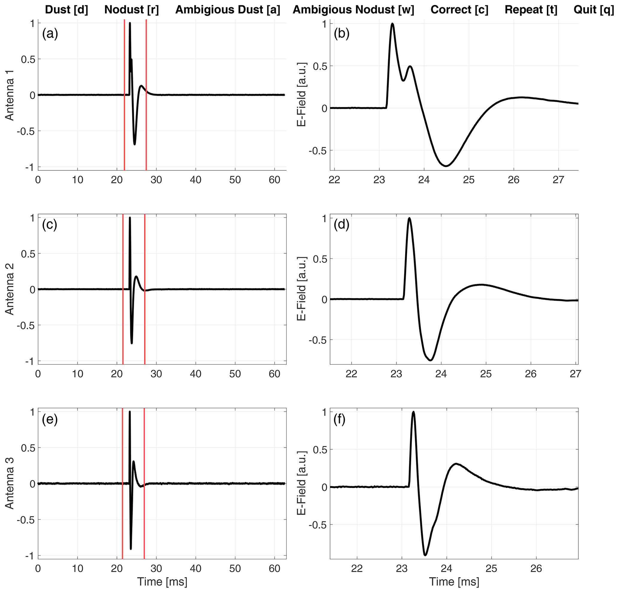
Figure A1 The manual labeling user interface showing a signal observed 28 July 2021. (a), (c) and (e) display the full snapshot (from 0 to ∼ 63 ms) at all antennas. An area of interest is selected by adjusting the red vertical lines. (b), (d) and (f) display the signal within the area of interest. The signal can be labeled as dust by pressing the [d] key on the keyboard and no dust by pressing the [r] key. The signal is indicated to be ambiguous if the waveform does not fit clearly into either of the two labels; note however that signals indicated to be ambiguous were also labeled into either dust or no dust using the [a] and [w] keys. There is also an option to correct [c] the previously labeled signal (in case of an error), repeat [t] the area of interest selection and quit [q] the manual labeling user interface.

Appendix B: The classification performance metrics

The classification performance metrics are calculated using the true positive (TP), true negative (TN), false positive (FP) and false negative (FN) values, defined by comparing the predicted classes and the manually labeled classes, illustrated in Fig. 10.

The overall accuracy of the classifier is the proportion of observations that were correctly predicted by the classifier. The accuracy is mathematically defined as

$$\begin{array}{}\text{(B1)}& \mathrm{Accuracy}={\displaystyle \frac{\mathrm{TP}+\mathrm{TN}}{\mathrm{TP}+\mathrm{TN}+\mathrm{FP}+\mathrm{FN}}}.\end{array}$$

Precision (in this case) is defined as the proportion of data points predicted by the classifier as dust, whose “true” label is indeed dust. Precision is therefore calculated as

$$\begin{array}{}\text{(B2)}& \mathrm{Precision}={\displaystyle \frac{\mathrm{TP}}{\mathrm{TP}+\mathrm{FP}}}.\end{array}$$

Recall (in this case) is the proportion of observations manually labeled as dust, that were correctly predicted as dust by the classifier. Recall is defined as

$$\begin{array}{}\text{(B3)}& \mathrm{Recall}={\displaystyle \frac{\mathrm{TP}}{\mathrm{TP}+\mathrm{FN}}}.\end{array}$$

The F1 score acts as a weighted average of precision and recall and is calculated as

$$\begin{array}{}\text{(B4)}& \mathrm{F}\mathrm{1}=\mathrm{2}\left({\displaystyle \frac{\mathrm{Precision}\cdot \mathrm{Recall}}{\mathrm{Precision}+\mathrm{Recall}}}\right).\end{array}$$