Spatio-temporal development of large-scale auroral electrojet currents relative to substorm onsets

During auroral substorms, the electric currents flowing in the ionosphere change rapidly, and a large amount of energy is dissipated in the auroral ionosphere. An important part of the auroral current system is the auroral electrojets whose profiles can be estimated from magnetic field measurements from low-earth orbit satellites. In this paper, we combine electrojet data derived from the Swarm satellite mission of the European Space Agency with the substorm database derived from the SuperMAG ground magnetometer network data. We organize the electrojet data in relation to the location and time of the onset and obtain statistics for the development of the integrated current and latitudinal location for the auroral electrojets relative to the onset. The major features of the behaviour of the westward electrojet are found to be in accordance with earlier studies of field-aligned currents and ground magnetometer observations of substorm temporal statistics. In addition, we show that, after the onset, the latitudinal location of the maximum of the westward electrojet determined from Swarm satellite data is mostly located close to the SuperMAG onset latitude in the local time sector of the onset regardless of where the onset happens. We also show that the SuperMAG onset corresponds to a strengthening of the order of 100 kA in the amplitude of the median of the westward integrated current in the Swarm data from 15 min before to 15 min after the onset.

1 Introduction

Ionospheric electric currents give rise to a variety of space weather effects that influence the performance and reliability of space-borne and ground-based technological systems. Problems in ground-based systems occur, for instance, due to geomagnetically induced currents (GIC) in technological conductor systems such as power grids (Pirjola, 2000, 2002). Substorms are a major source of GIC (Viljanen et al., 2006) because the geoelectric fields and induced currents are linked to rapid changes in the ionospheric currents, which are highly variable during substorms. A better understanding of the temporal and spatial structure of the high-latitude ionospheric currents during substorms, in particular a better description of their contribution for a given time and location, is therefore of great importance not only for advances in fundamental space research but also regarding practical applications.

Rostoker et al. (1980) gave a general definition of a magnetospheric substorm as “a transient process initiated on the nightside of the earth in which a significant amount of energy derived from the solar wind–magnetosphere interaction is deposited in the auroral ionosphere and in the magnetosphere” and, more specifically, as a time interval in which most of the energy dissipation is confined to the auroral oval. Following the definition of Rostoker et al. (1980), the onset of the substorm is associated with a large increase in auroral luminosity in the midnight sector of the auroral oval. The development of the aurora at the onset time and during substorms was first described by Akasofu (1964), who determined that, despite the variability from substorm to substorm, there are common substorm features, such as the formation and expansion of the bulge poleward, westward and eastward. Another prevalent phenomenon linked to substorms is the formation of the substorm current wedge (SCW). Bonnevier et al. (1970), Horning et al. (1974) and McPherron et al. (1973) established that the SCW is an integral part of substorm physics. The magnetic field signature of the enhanced currents related to the SCW can be observed from the ground, and the signature also provides a way of identifying substorms and substorm onsets in principle without direct observations of the aurora (Newell and Gjerloev, 2011a; Forsyth et al., 2015). The SCW has been and still is an active research topic (see Kepko et al., 2015, for a review). Ohtani et al. (2021b) found evidence that the nightside subauroral magnetic signatures of substorms can be attributed to the SCW. Recently, the open question of the possible role of small-scale wedgelets in forming the large-scale SCW has also gathered attention (Liu et al., 2015; Nishimura et al., 2020; Ohtani and Gjerloev, 2020; Orr et al., 2021).

The statistical behaviour of the aurora, the enhanced field-aligned currents (FACs) linked to the aurora, and the SCW and the horizontal ionospheric currents related to the SCW have been studied extensively. Gjerloev et al. (2007) used satellite observations in the ultraviolet to perform a statistical study of the auroral features described by Akasofu (1964) and obtained a quantitative description of the development of the bulge and the oval aurora. Ohtani et al. (2021a) described the observations of double auroral bulges, Forsyth et al. (2018) studied the seasonal variation of FACs related to substorms from AMPERE (Active Magnetosphere and Planetary Electrodynamics Response Experiment) data and Coxon et al. (2014) also used AMPERE data to derive statistics of Region 1 and Region 2 FACs during substorms in relation to open magnetic flux. Gjerloev and Hoffman (2014) provided an empirical model of the equivalent current system at the peak of a bulge-type auroral substorm, and Orr et al. (2019) used a directed network analysis to estimate the evolution of the equivalent current pattern during substorms. In this study, we will use the divergence-free current calculated with the spherical elementary current system (SECS) method (Vanhamäki et al., 2003; Vanhamäki and Juusola, 2020) provided by the Auroral Electrojet and auroral Boundaries estimated from Swarm observations (Swarm-AEBS) data products from the European Space Agency's Swarm mission (Friis-Christensen et al., 2006). We combine the Swarm-AEBS data set with a SuperMAG substorm list (Gjerloev, 2012; Newell and Gjerloev, 2011a, b) to derive statistics for the divergence-free current linked to the auroral electrojets in relation to the substorm onsets. Statistics of the ionospheric currents using the SECS method and Swarm have been derived in previous studies from the viewpoint of hemispheric and seasonal differences (Workayehu et al., 2019, 2020). Using the Swarm data in the substorm context provided by SuperMAG will enable this study to focus on the substorm time divergence-free currents. Swarm also provides a different view of the currents compared with ground-based magnetometers, as the latitudinal coverage of the auroral oval crossing is not dependent on the network density, and the effect of ground-induced currents on the magnetometer measurements, which can sum up to tens of percent of the total field strength at ground level (Juusola et al., 2020), is subdued at Swarm altitudes.

In general, the horizontal ionospheric currents can be modelled as sheet currents on a spherical surface with a radius of R_E +110 km (Earth radius R_E=6371.2 km). In this thin-shell approximation (Untiedt and Baumjohann, 1993), the horizontal ionospheric sheet current density can be separated into two components: the curl-free part, connected to the FACs such that it closes the regions of upward and downward current, and the divergence-free part, forming a rotational current that closes within the ionospheric current sheet (Amm and Viljanen, 1999). The eastward electrojet (EEJ) in the dusk sector and the westward electrojet (WEJ) in the dawn sector are major features associated with the divergence-free system. These currents can be studied using the magnetic field observations from ground and space. Ground-based networks usually provide better spatial coverage and are able to separate spatial and temporal changes in the magnetic field, but the networks are relatively sparse and can only provide knowledge on the equivalent current pattern that corresponds to the divergence-free current. Observations made by satellites and satellite constellations such as Swarm, CHAMP (CHAllenging Minisatellite Payload; Reigber et al., 2002) and AMPERE (Anderson et al., 2000, 2002, 2014, 2018; Waters et al., 2001, 2004, 2020; Coxon et al., 2018), which orbit the Earth above the current sheet, can also provide observations about the FAC and the curl-free current system along the orbits, but the spatial coverage is usually more limited, and it can be difficult to separate spatial and temporal changes. Satellites in low earth orbit are still relatively close (i.e. < 500 km) to the ionospheric currents which enables them to provide information about the ionospheric current system in reasonable latitudinal resolution compared with the auroral oval extent. Signals from structures smaller than the distance between the satellite and ionosphere get strongly attenuated, as the magnetic field signature of divergence-free currents obey the Laplace equation (Amm and Viljanen, 1999). In particular, we can characterize the development of the substorm temporal statistics of the dominant features of the horizontal divergence-free currents and the auroral electrojets using Swarm data. The analysis is done for both the EEJ and the WEJ, and we obtain spatio-temporal statistics of the divergence-free current carried by auroral electrojets and their boundaries in relation to substorm onset time and location. The structure of the paper is as follows: the data and methods used are described in Sect. 2; the results are presented in Sect. 3; Sect. 4 contains discussion; and Sect. 5 summarizes the conclusions.

2 Data and methods

2.1 Satellite and ground-based data

Swarm is a three-satellite mission of the European Space Agency to study the Earth's magnetic field (Friis-Christensen et al., 2006). Two of the satellites (Alpha and Charlie) were launched to fly side by side with an initial orbital height of 430 km, whereas the third (Bravo) has an orbital height of 530 km. The Swarm-AEBS product is based on the measurements of the Vector Field Magnetometer (Merayo et al., 2008). We use the Swarm-AEBS product data for the Northern Hemisphere and for Swarm Alpha and Bravo. The data from Charlie are almost identical to those from Alpha; thus, using both Alpha and Charlie would most likely skew the statistics. Swarm-AEBS data contain the electrojet current density and boundaries derived with both the SECS method and the line current (LC) method (Olsen, 1996) as well as estimations of the oval boundaries from FACs (Xiong et al., 2014). In this study, we use only the SECS-based data to determine the integrated currents for auroral oval crossings and the locations of the maxima as well as the equatorward and poleward borders of the electrojets. The current densities have been derived with the one-dimensional (1-D) SECS method (Vanhamäki et al., 2003; Juusola et al., 2006). The 1-D SECS method is used to determine latitude profiles of the divergence-free current density, curl-free current density and field-aligned current density for each crossing of the auroral region. The electrojets are defined from the divergence-free part of the current. The analysis is performed in an orthogonal spherical coordinate system (Semi QD) whose pole is rotated to match the pole in the proper quasi-dipole (QD) coordinates (Richmond, 1995; Emmert et al., 2010), which are very useful for organizing data but do not provide an orthonormal basis for the analysis. In this set-up, the divergence-free current is orientated zonally in the Semi QD coordinate system. However, when we bin the location of the electrojets, we use the QD latitude of the points in question. The electrojets are identified by locating the sign changes in the current density for each oval crossing profile. The latitude values of the sign changes are then used to integrate the profile in the meridional direction in the Semi QD coordinate system between two consecutive sign changes. Thus, the operation is a line integral along a meridian on the surface of a sphere with a radius of 6481 km, which is the distance from the centre of the Earth, where the currents are assumed to flow. The WEJ limits are then defined as the coordinates of the sign changes between which the integrated value is most negative, and the EEJ limits are the coordinates of the sign changes between which the integrated value is most positive. The peak value is then searched for within both the EEJ and WEJ limits separately. For more details on the detection method, we refer the reader to Kervalishvili et al. (2020). Figure 1 shows an example of the divergence-free current density for an auroral oval crossing with the detected electrojets. The figure also shows other areas of current in addition to the main electrojets. As mentioned earlier, only the sequences with the most positive and most negative integrated current values are defined as electrojets in the context of this study. Figure 1 also demonstrates that even though the current values are sampled to match the 1 Hz magnetic field measurements used as input data, the 1^∘ SECS pole separation provides the scale limit for features in the current.

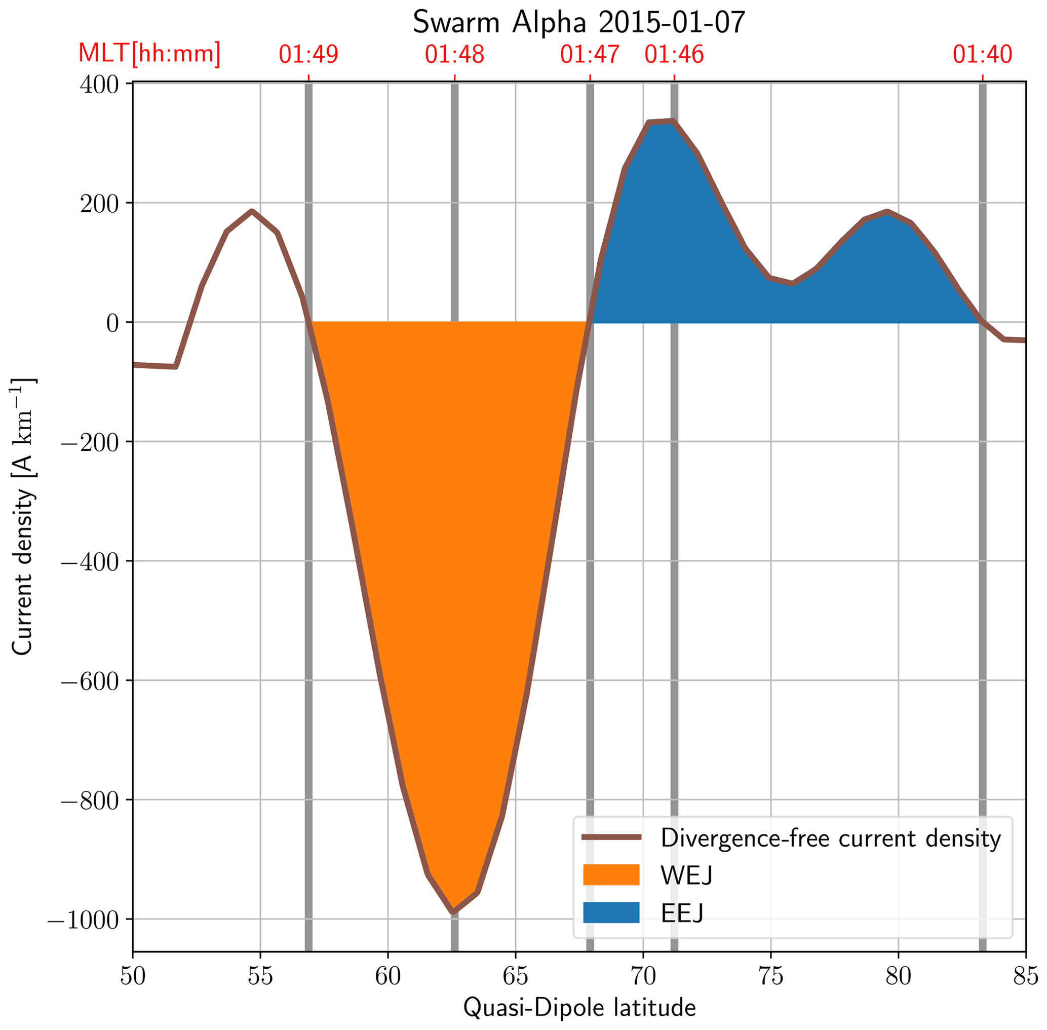
Figure 1 An example of the divergence-free current derived from Swarm Alpha data with the 1-D SECS method and the identified electrojets from the Swarm-AEBS data set. The location of the boundaries and maxima have been marked with vertical lines. The coloured sections show the area corresponding to the integrated currents.

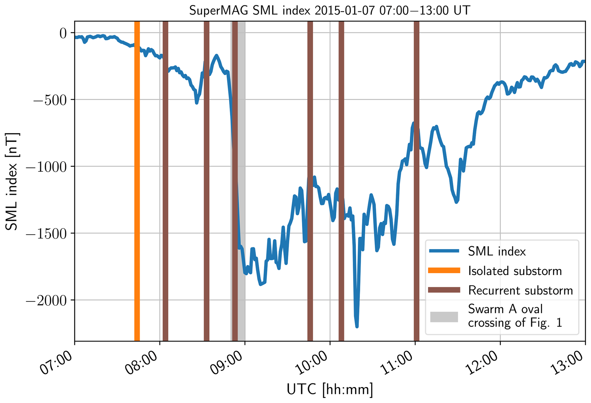
The SuperMAG substorm list (Gjerloev, 2012; Newell and Gjerloev, 2011a, b) is based on measurements from the SuperMAG ground magnetometer network (Gjerloev, 2012). The list is based on the SuperMAG AL index (SML), which is an auroral electrojet index derived from the SuperMAG data. It is similar to the AL index (Davis and Sugiura, 1966) with the biggest difference being the much greater number of stations used. The latitude and magnetic local time (MLT) coverage of the stations enable the identification of the time, MLT and latitude of the onsets without visual data. Another advantage of SuperMAG-based substorm identification is that data availability matches well with the lifetime of Swarm. However, even though the number of SuperMAG stations is large, ocean areas are obviously not well covered, and the onset location is naturally dependent on the position of the contributing magnetometers. The onsets in the substorm list have been shown to be highly correlated with a rise in auroral power (Gjerloev, 2012; Newell and Gjerloev, 2011a, b), and the list gives us a temporal relation between the currents and oval boundaries from Swarm measurements and onset parameters (see Figs. 1 and 2). We note that substorms derived using the SOPHIE (Substorm Onsets and PHases from Indices of the Electrojet) method could also be used (Forsyth et al., 2015).

Figure 2 An example time series of the SML index with the isolated and recurrent substorm onsets marked with vertical lines. The grey shading shows the relation of the oval crossing of Fig. 1 to the SML time series.

2.2 Identifying relevant auroral electrojet parameters and isolated substorm onsets

The QD latitude and MLT were calculated for the SuperMAG substorm onsets to match the data with the Swarm-AEBS data. From the onset list, we selected all substorm onsets that were more than 2.5 h from the previous one and in the MLT sector between 18:00 and 6:00, including the midnight. The 2.5 h limit is close to what Freeman and Morley (2004) obtained for the periodicity of substorms under constant solar wind driving in their minimal substorm model. We believe that this selection gives us the possibility to interpret the times before these onsets as a quieter baseline compared with the times near and after the onsets. Apart from this definition of isolation, we do not have any categorization for different scenarios of substorm occurrence (i.e. globally quiet or disturbed magnetospheric conditions or verification of the type of expansion by visible auroras). Figure 2 shows an example of a time series of the SML index and the related substorm onsets in relation to the oval crossing in Fig. 1. We do not distinguish cases where there are no recurrent onsets after the initial one from onsets that are followed by recurrent activity.

In order to relate the onset parameters to the Swarm-AEBS data, we associate timestamps and MLT values with the integrated current values and latitudinal extents for each auroral oval crossing in the Swarm-AEBS data. To do this, we use the mean time and MLT sector of the observations which cover the detected electrojets. Because the satellites can cover a large MLT sector close to the poles, the parameters were determined separately for the WEJ and the EEJ. The MLT range covered by a single oval crossing can exceed 2 h in some cases. We have used all oval crossings for the time period from 25 November 2013 to 31 December 2019 in the Northern Hemisphere where both the EEJ and WEJ are identified well, i.e. corresponding to the best possible quality flag (Kervalishvili et al., 2020). In practice, this means that both the boundaries and the peaks of the electrojets are well defined between the expected auroral electrojet latitude range from 50 to 85^∘ QD latitude and that the satellite path covers the QD latitudes from 50 to 85^∘. Altogether, the statistics are calculated from roughly 8430 oval crossings that fulfil our selection criteria. The crossings cover 2976 onsets from the SuperMAG onset list. For each onset, we calculated the MLT and QD latitude so that we could compare the oval crossing parameters to the onsets. The mean MLT and QD latitude of the onsets were 0.15 decimal hours and 67.3^∘ respectively. The integrated WEJ and EEJ values as well as the locations of the maxima and latitudinal extents (see Fig. 1) were then binned in 2 h bins of MLT difference from the onset MLT and 15 min bins with respect to the time difference from the relevant substorm onset. The evolution of the parameters of interest are then inferred from the median and percentiles in each bin. We also further separate the pre-midnight and post-midnight onsets to study the dependence of the data on the MLT of the onset around the onset time.

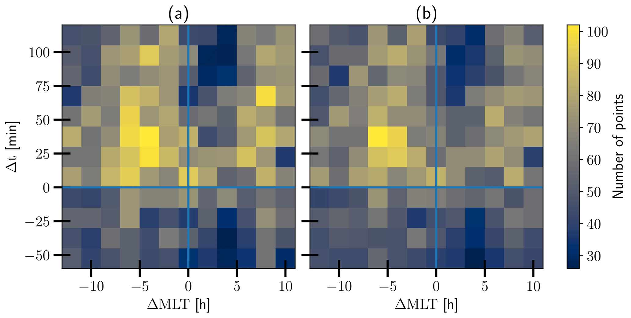
The binning was chosen to be reasonable with the fact that the SECS method assumes temporally stationary conditions for the duration of the oval crossing (about 10 min) and that divergence-free currents are calculated from measurements of the whole oval crossing. We acknowledge that this limits the interpretation of the results to these specific scales. In doing this, we also assume that the integrated currents and the averaged timestamp and MLT sector assigned to it are consistent with each other. Figure 3 shows the number of data points in each bin.

Figure 3 The number of Swarm oval crossings in each bin for the WEJ (a), corresponding to panels a and c in Fig. 4, and for the EEJ (b), corresponding to panels b and d in Fig. 4. ΔMLT is the magnetic local time distance to the onset, and Δt is the temporal distance to the onset.

3 Results

3.1 General development of the median integrated currents

Figure 4 shows the general development of the median integrated WEJ (panel a) and EEJ (panel b) with respect to the MLT difference and temporal offset to the substorm onset. Panels c and d show the ratio of each median compared to the last median before the onset of the same ΔMLT bin (panel c for the WEJ and panel d for the EEJ). For the sake of clearer presentation, we have highlighted two MLT sectors in both panels: W1 and W2 in Fig. 4a and c for the WEJ and E1 and E2 in Fig. 4b and d for the EEJ. Sector W1 stands for 1 h west (towards smaller ΔMLT values) to 5 h east (towards larger ΔMLT values) of the onset, sector W2 stands for 1 to 5 h west, sector E1 stands for 11 to 3 h west and sector E2 stands for 3 h west to 3 h east. Figure 4a and b show that the binning organizes the WEJ data better than the EEJ data. As the substorm onset MLT locations in the SuperMAG list are focused heavily around the nightside, we observe traces of the dawn and dusk electrojets in sectors W1 and E1 respectively before the onset (i.e. the negative temporal difference portion of the plot). A strengthening in amplitude of the WEJ median (corresponding to more negative values) after the onset is clearly visible in sectors W1 and W2. The maximum absolute values of the WEJ are observed 30 to 90 min after onset. The medians reach values of about 2 to 3 times the values before the onset, and the absolute values of the integrated current in sector W1 can be seen to be about 2 to 2.5 times greater in amplitude than the values in sector W2. The greatest relative increase in the eastward current in Fig. 4b and d can be seen in sector E2 after the onset, but the current also increases in sector E1. The intensification in E2 seems to reach the maximum eastward extent only after 15 to 30 min following the onset, and the values mostly reach 2 to 2.5 times the values before the onset. We will return to the difficulty of interpreting the EEJ results in Sect. 4.3.

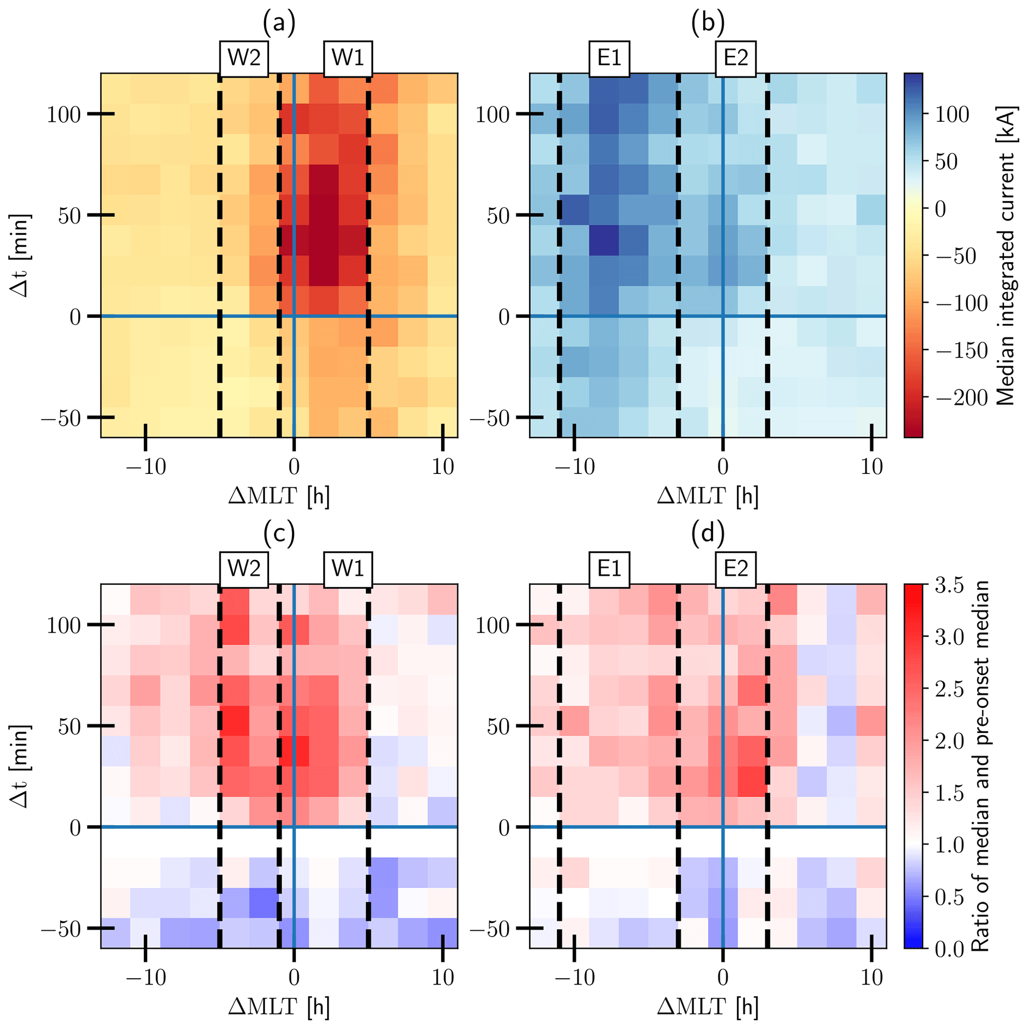
Figure 4 The development of the median integrated westward (a) and eastward (b) current binned with 15 min bins with respect to the temporal difference from the substorm onset and with a 2 h bin with respect to the MLT difference from the onset. Panels (c) and (d) show the ratio of the medians in panels (a) and (b) compared with the value just before the onset. The dashed vertical lines show the extent of sectors W1, W2, E1 and E2.

3.2 Statistics of the WEJ and EEJ integrated currents and latitudinal extent

In order to have a more robust view of the binned electrojet currents, we also present figures of the medians and the ranges containing the second and third quartiles (when we refer to the range from here onward, we specifically mean the range defined like this) of the data overlapped with the plots of the previous time step for the period from 30 min before the onset to 75 min after the onset in Figs. 5 and 6. Fig. 5a shows that the distributions of the consecutive time steps are very similar. Comparing the last and first time bins before and after the onset in Fig. 5b, we observe a clear increase of approximately 50–150 kA in the magnitude of the WEJ median and both the upper and lower quartiles, mostly in the W1 and W2 sectors. Figure 5c shows that the median continues to strengthen in the eastern part of sector W1 (i.e. 1 to 3 h east of the onset) from 15 to 30 min after the onset, but the effect is wider in the lower quartile, extending completely through both sectors W1 and W2. After 30 min, there is a well-defined sector of strong westward current in the W1 sector, with the integrated current median values reaching between −200 and −250 kA. The median values and ranges in sector W2 never drop below −125 kA. From 30 min following the onset (panels d, e and f) there is very little change in the medians, but the quartiles show the large variability in the data, with the lower quartile reaching values of roughly −360 kA.

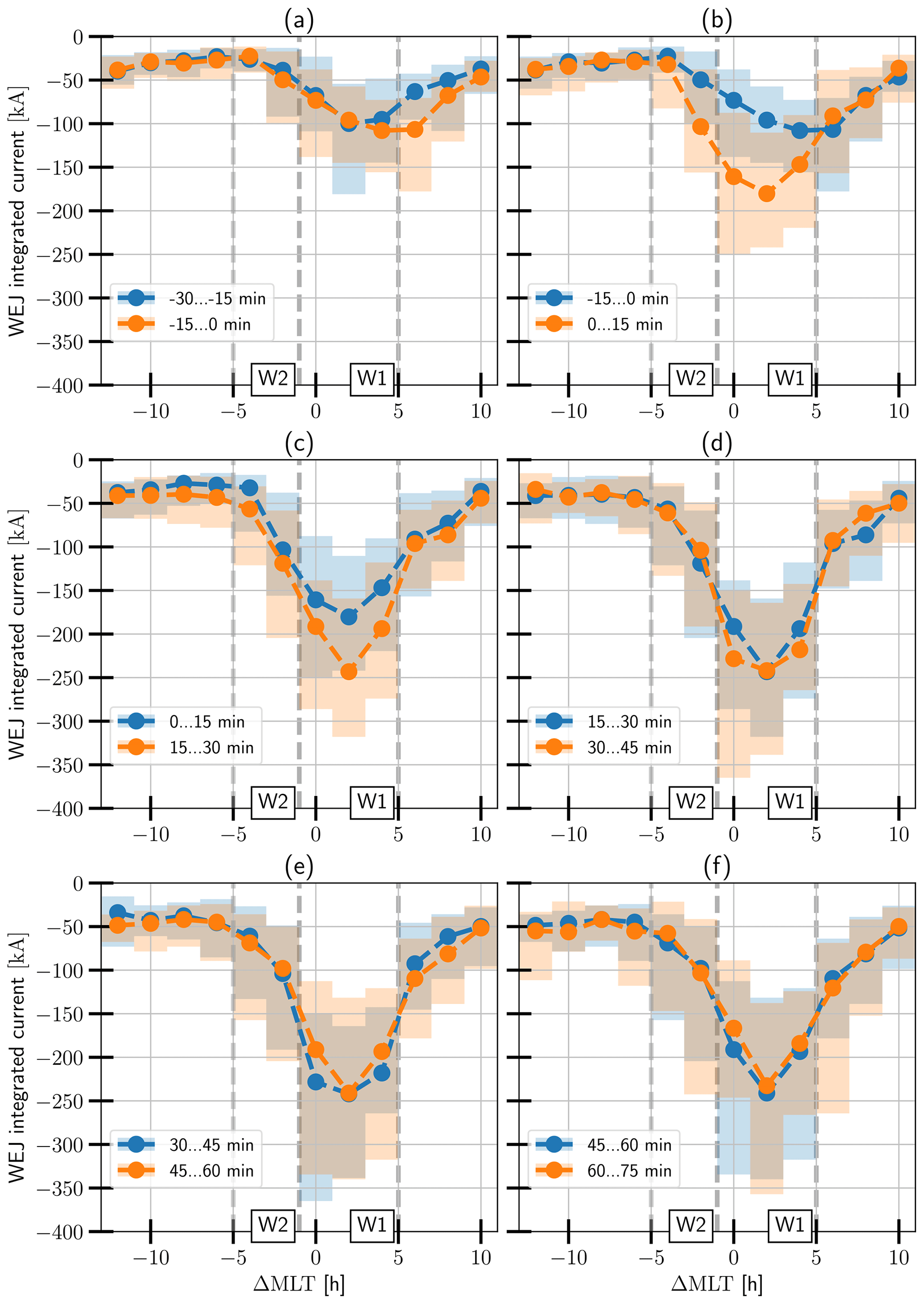
Figure 5 The evolution of the WEJ compared with the previous time step for the time period from 30 min before to 75 min after the onset. The lines show the medians, and 50 % of the values are contained within the bars in each bin.

The statistics of the EEJ in Fig. 6a show no clearly interpretable development of the distribution. Figure 6b shows the development of a second maximum of the EEJ near the onset location in sector E2 in addition to the initial peak in sector E1 which is formed dominantly from the signature of the dusk-side EEJ. The magnitude of this peak is rather small, as the median reaches only 75 kA. This double-peak structure in the median persists in Fig. 6c, but the peak in sector E2 is more concentrated around the middle of the sector, as the integrated values rise mostly in the middle and eastern parts of the sector. In Fig. 6d, e and f, the double-peak structure is still present, but the level of large-scale organization seems to be decreasing with positive and negative changes both in the medians and ranges in multiple ΔMLT sectors. The largest EEJ values are located in sector E1, with the upper quartile reaching maximum values of a little over 200 kA.

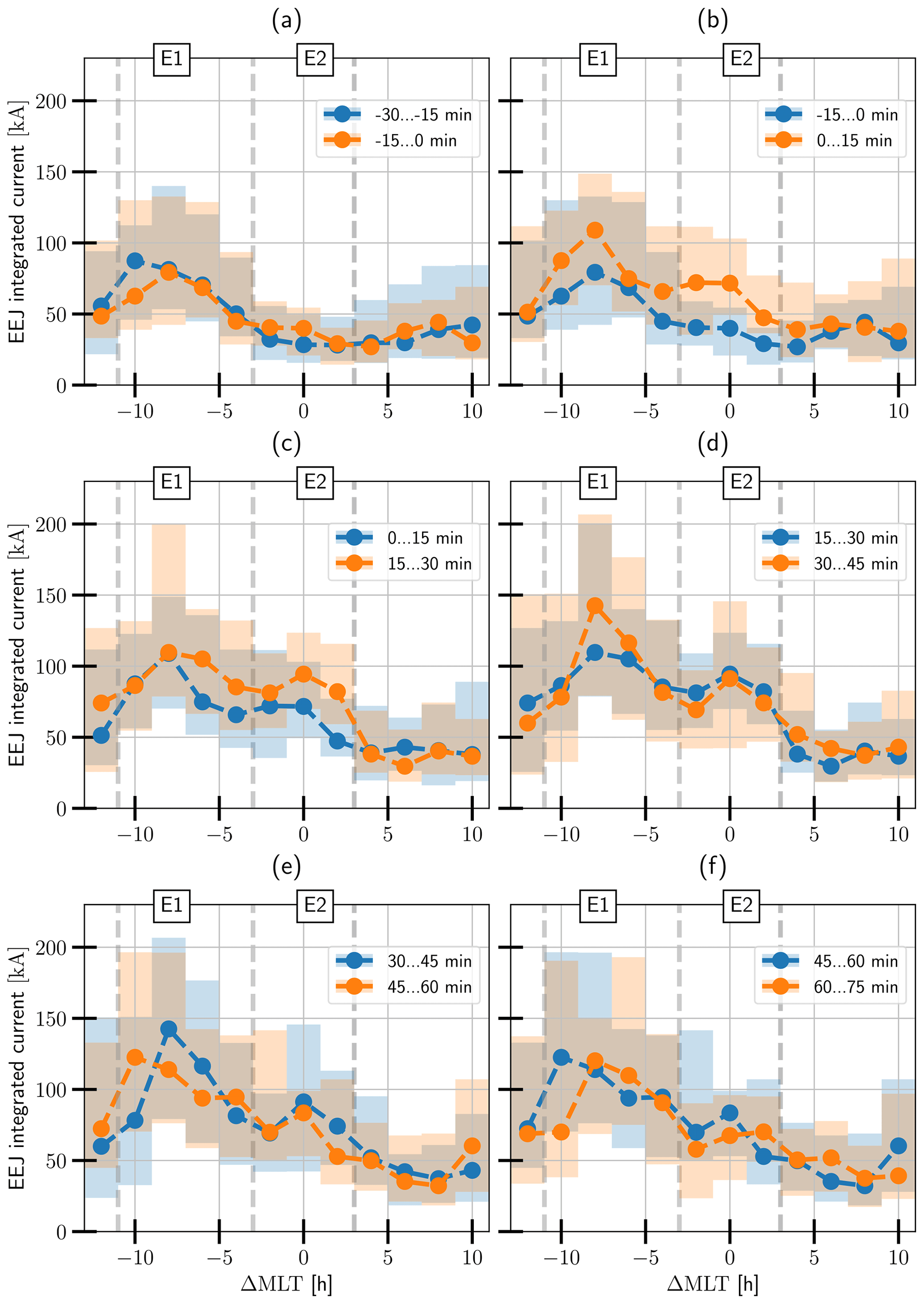
Figure 6 The evolution of the EEJ compared with the previous time step for the time period from 30 min before to 75 min after the onset. The lines show the medians, and 50 % of the values are contained within the bars in each bin.

Figures 7 and 8 show the medians and ranges for the location of the electrojet with respect to the onset latitude. The shape of the WEJ latitudinal extent as a function of ΔMLT in Fig. 7 is unsurprisingly reminiscent of the shape of the auroral oval of the westward-flowing current. The shape of the oval of the eastward current can be seen west of the onset in Fig. 8. Looking at Fig. 7, we see that the location of the WEJ in sector W1 is quite well centred near the onset latitude at the onset location and around 1^∘ poleward of the onset location after the onset time. Figure 7c, d and e show that the peak currents seen in sector W2 are located approximately 2 to 4^∘ poleward of the onset sector currents, whereas the W1 sector currents are located consistently closer to the onset latitude. The equatorward and poleward extent indicate a poleward movement of the order of 1 to 2^∘ in the WEJ position after the onset just west of the onset in sector W2. However, keeping in mind that the SECS method resolution is at most 1^∘ in either direction, there is uncertainty in the significance of the observation. Figure 8a shows how the EEJ in sector E1 is located poleward of the onset latitude but is clearly located more equatorward close to the onset location. It is also evident that the enhanced EEJ values in the eastern part of sector E2 in Fig. 6 are mostly located poleward of the onset location and the WEJ. In sector E2, the median values of the maximum as well as the poleward and equatorward extents of the EEJ location move sharply around 5^∘ poleward at the western end of the sector after the onset in Fig. 8b. However, the medians are located 5^∘ equatorward of the pre-onset position on the extreme western edge of the sector in panels c, d, e and f. While the ranges reveal that the data in these panels include EEJ structures similar to the medians in panel b and vice versa, the sharp jump in the median location persists but is now located in the middle of sector E2. This sharp edge of over 5^∘ is in contrast with the smoother poleward transition of the medians in panel a. This is most likely caused by the enhanced WEJ dominating the E2 sector so that the EEJ is found either poleward or equatorward of the WEJ, which naturally leads to this splitting of the distribution into two populations.

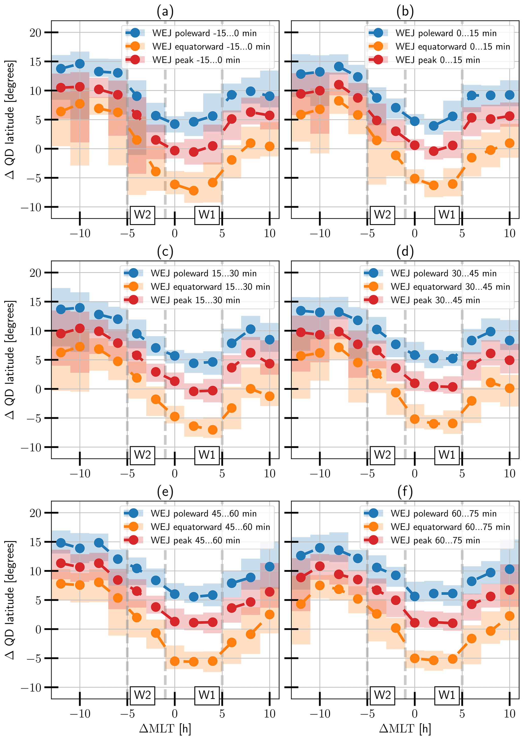
Figure 7 The evolution of the WEJ peak location and extent for the time period from 15 min before to 75 min after the onset. ΔQD is the latitude relative to the onset latitude. The lines show the median, and the shading shows the range covered by the second and third quartiles.

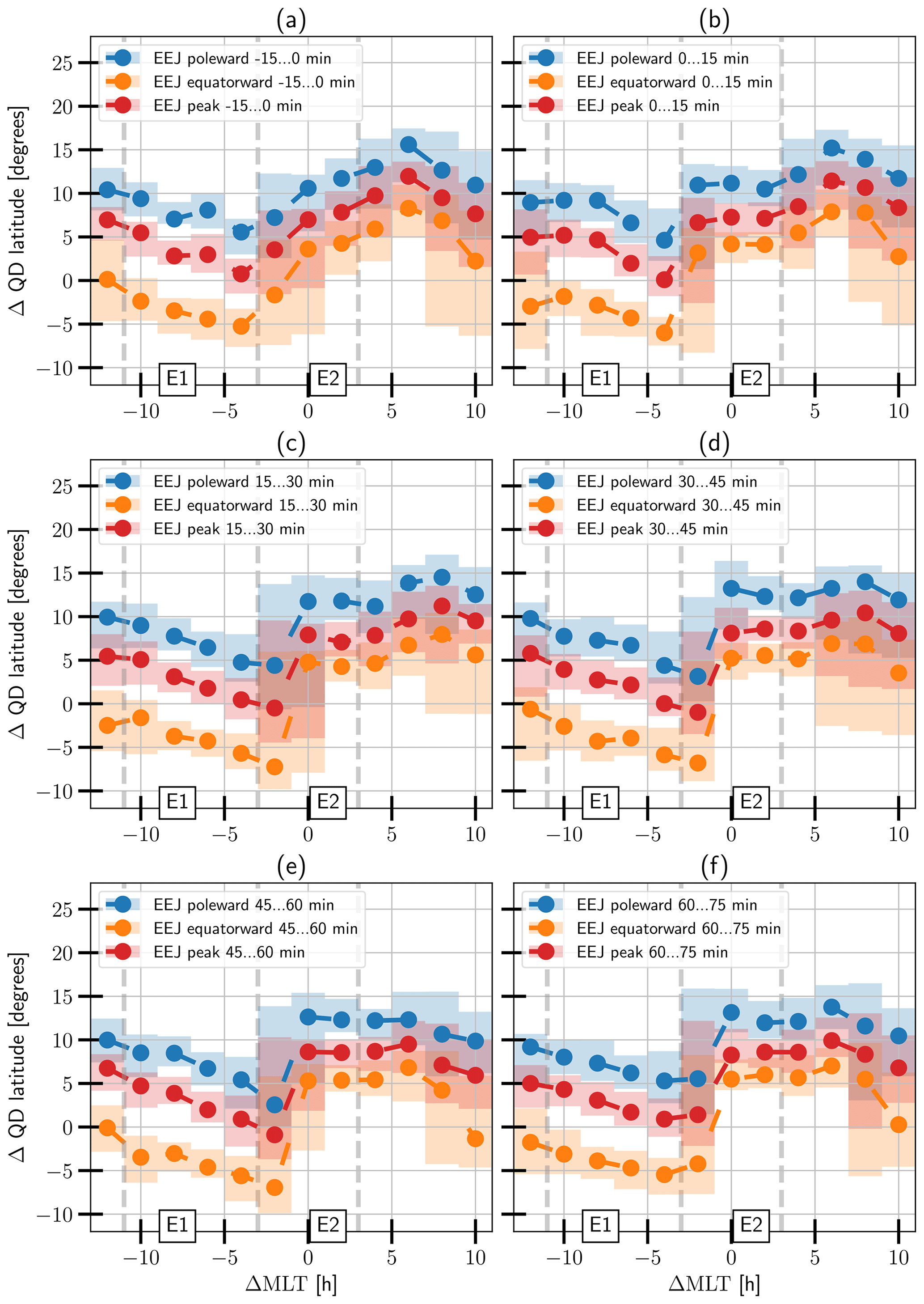
Figure 8 The evolution of the EEJ maxima location and extent for the time period from 15 min before to 75 min after the onset. ΔQD is the latitude relative to the onset latitude. The lines show the median, and the shading shows the range covered by the second and third quartiles.

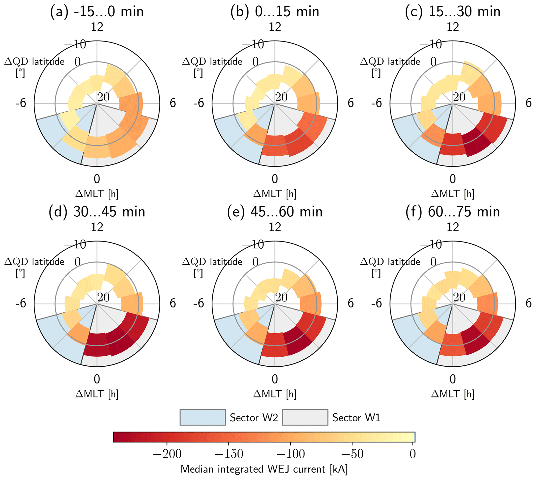
Figure 9 The temporal evolution of the WEJ median current and extent of the jet in polar (ΔQD,ΔMLT) coordinates.

To sum up the median behaviour of the WEJ data, we present the combined temporal development of the current and the location of the WEJ in Fig. 9, which illustrates that the W1 sector currents are greater than the W2 currents and that the jet in sector W1 is positioned around the onset location in contrast to the poleward position of the jet in sector W2. The apparent poleward displacement of the median WEJ location after the onset on the eastern edge of sector W2 is also visible.

3.3 Dependency of WEJ parameters and evolution on the onset MLT

Figure 10 shows the WEJ latitude location and MLT data from the 2 h MLT bin centred on the onset MLT (i.e. the ΔMLT=0 bin) and the time step corresponding to the period between 0 and 15 min after the onset. We see that although the onset MLT distribution is spread out, the point distribution is consistently such that the ΔQD=0 is close to the peak values and between the equatorward and poleward borders for onsets between 21:00 and 6:00. However, for onsets between 18:00 and 21:00, the peak location moves poleward of the onset MLT, and the furthest duskward jets are located nearly completely poleward of the onset, although the number of cases is low in this sector. It is possible that the poleward displacement is a signature arising from the Harang discontinuity (Koskinen and Pulkkinen, 1995). Figure 10 also shows that the latitudinal extent of the WEJ is larger on the dawn side compared with the dusk side. We believe this is because the WEJ is generally better established on the dawn side. The Harang discontinuity could also be an explanation for the equatorward extent of the WEJ moving poleward in the dusk sector. For comparison with the substorm time results, we also checked 1797 oval crossings that were within 1 h west and 1 h east of the SML value with any temporal distance to any substorm. For this check, we also required that the SML MLT was between 18:00 and 6:00. The latitudinal position distribution of the WEJ maximum was found to be centred around the SML QD latitude. The median difference between the WEJ maximum and the SML QD was 0.5^∘ poleward. However, unlike in the substorm time crossings shown in Fig. 10, there were several outliers far away from the SML QD latitude.

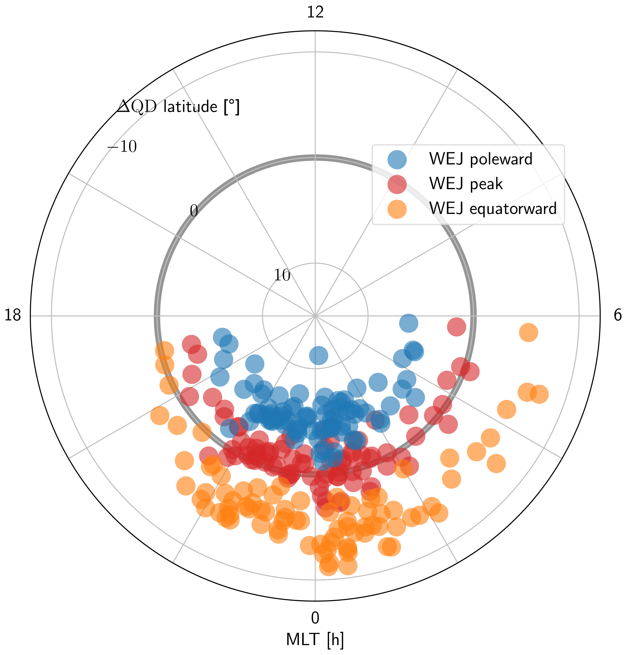
Figure 10 The MLT and ΔQD latitude locations of the WEJ peaks as well as the poleward and equatorward borders in the 2 h MLT bin centred around the onset location 0 to 15 min after the onset. ΔQD is the latitude relative to the onset latitude.

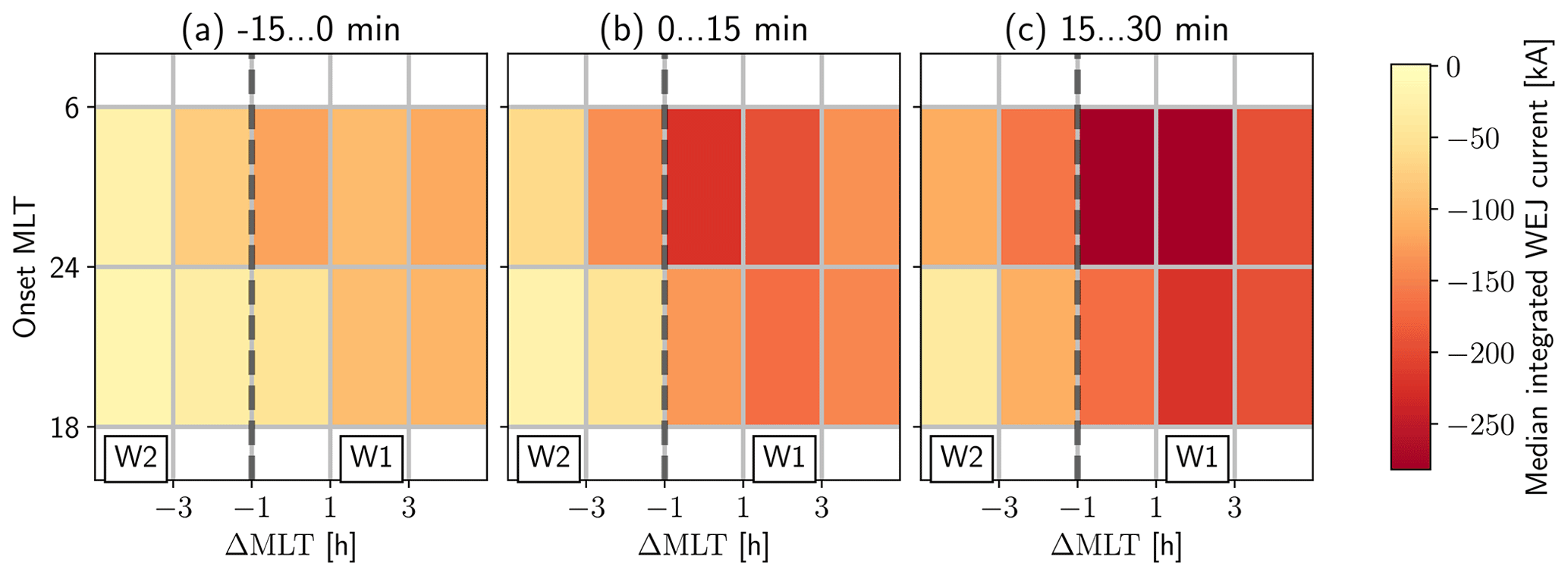
Figure 11 The temporal evolution of the median WEJ before and after the onset separated for pre-midnight onsets and post-midnight onsets. The top row shows the values for post-midnight onsets, and the bottom row shows the values for the pre-midnight onsets.

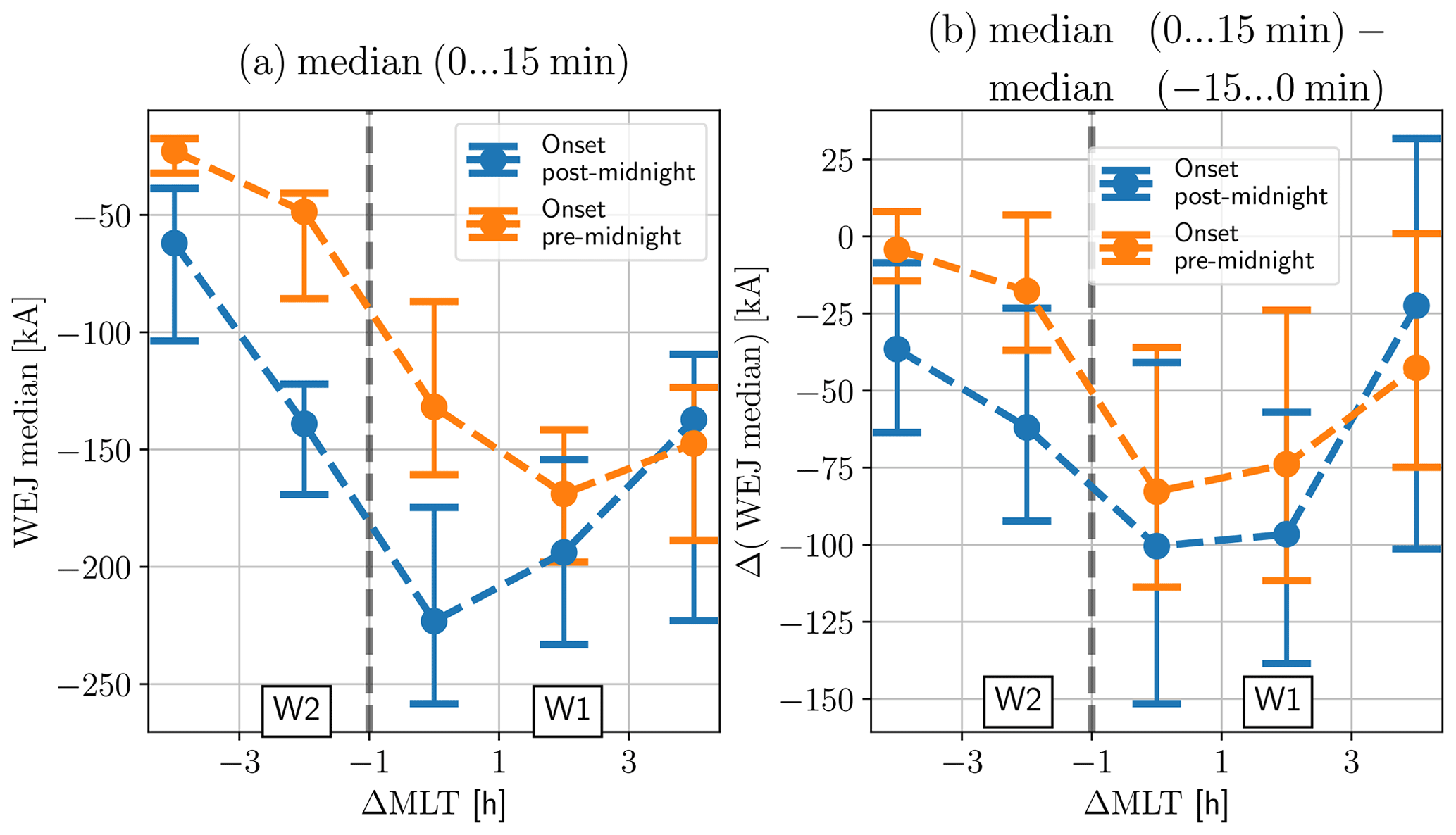
Figure 12 The median WEJ after the onset and the difference in the median WEJ between time steps before and after the onset separated for pre-midnight onsets and post-midnight onsets as well as bootstrapped 90 % confidence intervals.

To study the amplitude evolution, we divided the data into pre-midnight onsets and post-midnight onsets. Of the 2976 onsets, 1411 are located post-midnight and 1565 are located pre-midnight. Figure 11 shows the median WEJ data covering sectors W1 and W2 but now separately for the two sets of onsets covering the time period between 15 min before and 30 min after the onset time. The three time steps together contain 1260 oval crossings in the pre-midnight onset group and 1087 oval crossings in the post-midnight onset group. The basic statistical nature of the MLT distribution of the oval WEJ underlies the changes in time, as the pre-midnight values are clearly smaller, and the pattern formed by the pre-midnight data is similar to the post-midnight data but shifted eastward. Figure 12a shows the same data as Fig. 11b. The 90 % confidence intervals shown in the figure were calculated using the bias-corrected and accelerated bootstrap method (BC_a) (Efron and Tibshirani, 1993, pp. 178–188; Chernick and LaBudde, 2011, pp. 85–88). The pre-midnight curve has a minimum east of the onset sector. By contrast, the post-midnight curve has a minimum within the onset sector. Figure 12b shows the bootstrap estimated difference in the medians, which were again calculated with the BC_a method, between the last bin before and the first bin after the onset (i.e. the difference between Fig. 11b and a). The absolute value of the difference in the medians is greatest at the onset sector and the centre of sector W1 for both the pre-midnight and the post-midnight curves, with values of roughly 80 kA for pre-midnight onsets and 100 kA for post-midnight onsets. The pre-midnight values catch and take over the post-midnight values at the eastern edge of sector W1.

4 Discussion

Because of the local nature of the Swarm observations, we must emphasize that our statistics consist of observations from different substorms at different locations in time and space and not from full-coverage observations of temporally evolving substorms. However, it is meaningful to interpret the statistics in relation to the physics of substorms through existing theories and compare the results with other studies. Following previous studies, we will comment on the timing and expansion aspects of the data set. We concentrate on the WEJ because of its clearer relation to the SCW. We also note that the timescale and 1-D method used in our analysis mean that our results consider mostly the large-scale WEJ and cannot give information on wedgelet-type structures.

4.1 Temporal development of the amplitudes

To interpret the temporal development of our results, we must note that it would be beneficial to use a normalized timescale in a similar fashion to Gjerloev et al. (2007), in order to avoid mixing the expansion and recovery phases of substorms in a statistical study. For example, Orr et al. (2019) also used the same normalized timescales. However, as the Swarm oval crossings provide only snapshots of substorms from certain MLT sectors, it is not possible to avoid this mixing when working with Swarm data alone, and we have to keep this in mind when looking at the MLT distribution of the currents at different times. Gjerloev et al. (2007) obtained approximately 30 min as the mean duration on the expansion phase, and we can use this information to roughly assume that on average the bins from 0 to 15 and from 15 to 30 min are mostly samples of the expansion phase of the substorms, whereas the bins after the 30 min mark are a mix of samples from the expansion and recovery phases as well as recurrent substorm activity after the initial onset. This is supported by the large-scale organization of the temporal behaviour in Fig. 5b and c, which show general strengthening of the medians as well as the lower and upper quartiles. By contrast, the medians are stable, but the ranges between quartiles are large from the 30 min mark onward in Fig. 5d, e and f, showing the mixing of different phases in observations.

Our observation of the median and the ranges of the WEJ reaching values close to their maximum values at 15–30 min after the onset is consistent with the observations of Coxon et al. (2014), who found maximum values for Region 1 and Region 2 FACs and their ratio. Forsyth et al. (2018) also observed similar timescales for the average Region 1 and Region 2 FACs to reach their maximum values. We conclude that the timescales for WEJ intensification coincide quite well with the FAC timing obtained from the global AMPERE observations.

4.2 The WEJ amplitude and location in relation to the SCW and bulge-type expansion

Figures 5 and 7 show that the enhancement of the WEJ after the onset in sector W1 is located near or slightly equatorward of the onset latitude. In sector W2, the westward current is smaller in amplitude and is located 2 to 4^∘ poleward. The MLT sectors here are, of course, the edges of our bins and are not to be taken as precise limits for any physical phenomena. In light of the SCW theory and observations of the expansion of bulge-type substorms, it is likely that the distribution in sector W2 is formed mostly of Swarm passes through the substorm bulge and the westward-travelling surge. The W1 sector data, on the other hand, are formed of passes over the part of the SCW that flows along the auroral oval or the eastern part of the bulge. Previous studies supporting this interpretation include, for example, Kamide and Akasofu (1975), Gjerloev and Hoffman (2002), Gjerloev et al. (2007), and Fujii et al. (1994). We also note that the top currents in sector W1 and W2, especially in Fig. 5d, are similar to values obtained by Gjerloev and Hoffman (2002) for the respective bulge and surge in their model derived from Dynamics Explorer 2 satellite data (see Gjerloev and Hoffman, 2002, their Fig. 5). The latitudinal location of the observed WEJ in sectors W1 and W2 is qualitatively consistent with what could be expected from observations of satellite passes over a system depicted in Kepko et al. (2015) (their Fig. 9), which is based on observations from Fujii et al. (1994) and Gjerloev and Hoffman (2002). Gjerloev and Hoffman (2014) observed similar displacement and amplitude differences of the WEJ from SuperMAG data for the pre-midnight and post-midnight components of the electrojet determined from ground-based data of the SuperMAG network.

Figures 7 and 8 also provide a way to characterize the variability of the jet in a statistical sense. We can interpret the non-overlapping ranges of the locations of the poleward boundary, the peak and the equatorward boundary as a sign of a spatially and temporally stable jet in the chosen coordinate system, and we can interpret overlapping ranges as a sign of temporal and/or spatial variability in the system. Keeping this in mind, we see not only that the WEJ is very clearly defined in sector W1 throughout the studied period but also that the level of organization increases after the onset in sector W2. The lower level of organization in the duskward sectors with overlapping locations and large variability in the amplitudes may arise from the satellite observing variable substructures or structures moving in time instead of a more statically positioned large-scale jet as Kepko et al. (2015) anticipated.

The onset location is very well located inside the WEJ part of the oval and seems to always be quite close to the peak location, which can be seen clearly in Fig. 10. The distribution of the points shows the strong correlation between substorm onsets determined from the SuperMAG SML index and the WEJ profiles defined from Swarm data. This not surprising because the magnetic disturbances measured by the SuperMAG network should correspond to the ionospheric equivalent current which, in turn, should correspond quite well to the divergence-free current derived from Swarm; nevertheless, it is an indication that the SML index-based substorm detection does correlate with the enhanced westward divergence-free current with an electrojet-like profile centred on the location. Coxon et al. (2017) concluded that the substorm onset is co-located with the boundary of the Region 1 and Region 2 FACs which implies that the WEJ peak is also located close this boundary. Figure 11 shows that it is more likely to reach large currents if the onset location is in the post-midnight sector. This feature is the effect of the substorm enhancement being added to the pre-substorm WEJ which tends to be greater in the post-midnight sector. The actual median current value is clearly greatest at the onset location for the post-midnight onsets, whereas the WEJ intensities tend to peak eastward of the onset in the cases of pre-midnight onsets. We note that the statistical observation of the WEJ peak location differing from the onset location for pre-midnight onsets very likely arises from mixing different substorms and pre-substorm conditions and does not mean that the SML index would not probe the maximum of the WEJ. By contrast, the difference in the median before and after the onset shows the maximum enhancement occurring at the onset location for both pre-midnight and post-midnight onsets. It is likely that the differencing reduces the statistical effect of the underlying oval conditions and more successfully reveals the substorm enhancement.

4.3 Limitations of the analysis and interpretation

Looking at Fig. 3, it is obvious that the number of oval crossings per bin is far from ideal for statistical analysis, ranging from about 40 to 125. The distribution of points is not very uniform across the bins. It is also possible that our quality flag selection – allowing only cases where both the EEJ and WEJ are entirely between QD latitudes of 50 and 85 – causes systematic bias, as certain current systems are not represented in the data set. We also recognize that estimating currents from single-satellite magnetic field measurements with the SECS method involves solving an ill-posed inverse problem. Although SECS has been shown to give reasonable results in a statistical sense and in case studies (Juusola et al., 2007, 2016), some features in its output are affected by adjustments made in the inversion methodology for enhanced robustness in massive data analyses.

As mentioned in Sect. 3.2, the statistics show an enhancement of the EEJ in sector E2 after the onset, which seems to propagate eastwards. The enhancement is located mostly poleward of the WEJ, as can be seen from Figs. 8 and 7, and also coincides partly with the well-defined WEJ sector. However, it is not clear if this a physical phenomenon or an artefact arising from the limiting 1-D approximation (ignorance of longitudinal gradients) used in current single-satellite products. In Fig. 1, we see the current profile with quite symmetrical eastward bumps on either side of the westward current. We also note that because the SML index is associated with westward-flowing currents, the WEJ statistics are naturally more organized in our chosen coordinate system in general compared with the EEJ.

5 Conclusions

We have shown that the auroral electrojet characteristics derived from Swarm-AEBS data products are organized in a way that can be interpreted to be consistent with earlier observations of bulge-type substorm expansion and large-scale SCW development. Although the data consist of separate oval crossings from different sectors of substorm current systems, the resulting distribution agrees with earlier studies of the temporal development of substorms, at least in the 15 min timescale used in this study. The peak currents are mostly observed between 30 and 45 min after the onset. The Swarm-AEBS data reproduce the well-known poleward latitudinal displacement of the western part of the SCW in relation to the onset latitude and the eastern part of the SCW of about 2 to 4^∘. Simultaneously, we show the amplitude of the WEJ to be at least twice as large in the sector of 1 h west to 1 h east of the onset compared with values further than 1 h west of the onset. The results also place the onset location determined by the SuperMAG method within the WEJ determined from Swarm; thus, the latitude of the onset in the SuperMAG database correlates well with the peak location of the WEJ determined from Swarm-AEBS data set regardless of the onset location. We also show that the ΔMLT distribution of westward divergence-free currents between 0 and 15 min after the onset is different for post-midnight and pre-midnight onsets, which is most likely due to the variance caused by the underlying auroral oval conditions. However, the greatest temporal strengthening of the median WEJ coincides with the SuperMAG onset location for both post-midnight and pre-midnight onsets. Our study shows that, despite their different approaches, SuperMAG and Swarm-AEBS data products can give a coherent picture of the main features in the substorm current system. This finding encourages the combined usage of the two data sets in order to improve spatial coverage, resolution and uncertainty estimates in comparison with results derived from single-source data.