the Creative Commons Attribution 4.0 License.
the Creative Commons Attribution 4.0 License.
 | 10 Dec 2019
Long-term trends in the ionospheric response to solar extreme-ultraviolet variations
Rajesh Vaishnav
Christoph Jacobi
Jens Berdermann
The thermosphere–ionosphere system shows high complexity due to its interaction with the continuously varying solar radiation flux. We investigate the temporal and spatial response of the ionosphere to solar activity using 18 years (1999–2017) of total electron content (TEC) maps provided by the international global navigation satellite systems service and 12 solar proxies (F10.7, F1.8, F3.2, F8, F15, F30, He II, Mg II index, Ly-α, Ca II K, daily sunspot area (SSA), and sunspot number (SSN)). Cross-wavelet and Lomb–Scargle periodogram (LSP) analyses are used to evaluate the different solar proxies with respect to their impact on the global mean TEC (GTEC), which is important for improved ionosphere modeling and forecasts. A 16 to 32 d periodicity in all the solar proxies and GTEC has been identified. The maximum correlation at this timescale is observed between the He II, Mg II, and F30 indices and GTEC, with an effective time delay of about 1 d. The LSP analysis shows that the most dominant period is 27 d, which is owing to the mean solar rotation, followed by a 45 d periodicity. In addition, a semi-annual and an annual variation were observed in GTEC, with the strongest correlation near the equatorial region where a time delay of about 1–2 d exists. The wavelet variance estimation method is used to find the variance of GTEC and F10.7 during the maxima of the solar cycles SC 23 and SC 24. Wavelet variance estimation suggests that the GTEC variance is highest for the seasonal timescale (32 to 64 d period) followed by the 16 to 32 d period, similar to the F10.7 index. The variance during SC 23 is larger than during SC 24. The most suitable proxy to represent solar activity at the timescales of 16 to 32 d and 32 to 64 d is He II. The Mg II index, Ly-α, and F30 may be placed second as these indices show the strongest correlation with GTEC, but there are some differences in correlation during solar maximum and minimum years, as the behavior of proxies is not always the same. The indices F1.8 and daily SSA are of limited use to represent the solar impact on GTEC. The empirical orthogonal function (EOF) analysis of the TEC data shows that the first EOF component captures more than 86 % of the variance, and the first three EOF components explain 99 % of the total variance. EOF analysis suggests that the first component is associated with the solar flux and the third EOF component captures the geomagnetic activity as well as the remaining part of EOF1. The EOF2 captures 11 % of the total variability and demonstrates the hemispheric asymmetry.
- Article
(11555 KB) - Full-text XML
- BibTeX
- EndNote


The interaction of solar radiation with the ionosphere is complicated due to several mechanisms with the potential to modulate the thermosphere–ionosphere (T-I) system at different timescales ranging from the 11-year solar cycle down to minutes (e.g., Liu et al., 2003; Afraimovich et al., 2008; Liu and Chen, 2009; Chen et al., 2012). The ionosphere plasma response to solar EUV and UV variations has been widely studied using ground- and space-based observations (e.g., Jakowski et al., 1991; Jacobi et al., 2016; Schmölter et al., 2018; Jakowski et al., 1999), as well as by numerical and empirical modeling (e.g., Ren et al., 2018; Vaishnav et al., 2018a, b). These studies have shown that the response of the ionosphere to solar EUV radiation variations is delayed by 1–2 d at the 27 d solar rotation period (e.g., Jakowski et al., 1991; Afraimovich et al., 2008; Jakowski et al., 2002; Min et al., 2009; Jacobi et al., 2016; Lee et al., 2012).
To understand the underlying mechanisms of the delay observed in the ionospheric plasma, Jakowski et al. (1991) used a one-dimensional numerical model to explain the ionospheric delay of about 1–2 d. They concluded that the ionospheric delay could be attributed to the delayed atomic oxygen density variation at 180 km height produced via O2 photodissociation. Ren et al. (2018) performed multiple numerical experiments using the Thermosphere–Ionosphere Electrodynamics General Circulation Model (TIE-GCM) to investigate the potential physical mechanisms responsible for the ionospheric delay. Their simulation results revealed that photochemical, dynamic, and electrodynamic processes, as well as the geomagnetic activity, can be associated with the ionosphere response time. Vaishnav et al. (2018b) performed CTIPe model simulations to explore the dominant mechanisms and suggested that transport might be the leading process responsible for the ionospheric delay.
Apart from solar radiation, the T-I system is also influenced by different external forces, which include lower atmosphere forcing, particle precipitation, geomagnetic, and solar wind conditions (e.g., Min et al., 2009; Jakowski et al., 1999). As a result, the ionospheric plasma behavior is continuously varying depending particularly on the solar activity conditions. Lean et al. (2016) constructed a statistical model and characterized the spatial patterns of the ionospheric behavior at different timescales arising from the solar and geomagnetic conditions and showing annual and seasonal oscillations. Medium-term and long-term ionospheric variability, ionospheric storm time response, solar activity, and geomagnetic response were discussed by Kutiev et al. (2013).
The mean solar rotation period is approximately 27 d, and therefore similar periodic variations are expected in the ionospheric parameters, such as total electron content (TEC, measured in TECU: 1 TEC unit = 1016 electrons m−2), NmF2, etc. (e.g., Min et al., 2009). Hocke (2008) studied oscillations in the global mean TEC (GTEC) and solar EUV (Mg II index) and reported dominant periodicity at the timescale of the solar rotation and the annual, semi-annual, and solar cycles. These oscillations observed in GTEC could be related to the ionizing radiation changes. Kutiev et al. (2012) studied the middle- and low-latitude ionospheric response to solar activity. They suggested that the 27 d periodicity is the main dominant oscillation during the study period.
In order to understand the variability of the T-I system, the knowledge of solar EUV variations is essential. Since direct EUV measurements before the space age were not available due to atmospheric absorption, solar proxies have been frequently used to represent solar variability. The most widely used proxies for ionospheric applications are the F10.7 index (solar radio flux at 10.7 cm, measured in solar flux units, sfu; see Tapping, 1987, Maruyama, 2010), the Mg II index (the core-to-wing ratio of the Magnesium K line; Maruyama, 2010), and indices based on direct EUV measurements (e.g., Schmidtke, 1976; Unglaub et al., 2011; Jacobi et al., 2016) such as the Solar EUV Experiment (SEE, Woods et al., 2000) onboard the Thermosphere Ionosphere Mesosphere Energetics and Dynamics (TIMED) satellite. Using the latter poses the potential problem of satellite degradation (BenMoussa et al., 2013; Schmidtke et al., 2015), which may be overcome by repeated calibration or in-flight calibration as was applied during the SolACES experiment on board the ISS (Schmidtke et al., 2014, 2015). The understanding and realistic estimation of solar irradiance have been an open issue for long times, but in recent times the EUV datasets (either direct measurements, composite datasets, or models) have considerably improved (e.g., Haberreiter et al., 2017).
This paper investigates and evaluates the correlation between GTEC and different solar EUV proxies in the time period January 1999 to December 2017. The purpose of utilizing several proxies is to estimate the respective correlation and the ionospheric delay to identify proxies which are most suitable for describing the solar–ionosphere relationship at different timescales and under different solar activity conditions. Therefore, the ionospheric delay at the different oscillation periods of solar irradiance is addressed to investigate GTEC response to solar variations as indicated by various solar proxies. To understand the variability in the ionosphere, we use the method of empirical orthogonal functions (EOFs) in order to classify the temporal and spatial variability in the ionosphere.
Global TEC maps for the period 1999 to 2017 are available from the International Global Navigation Satellite Systems (GNSS) Service (IGS, Hernández-Pajares et al., 2009). We used NASA's 2-hourly global TEC maps, which are available in IONEX format from the CDDIS (ftp://cddis.gsfc.nasa.gov/gnss/products/ionex/, last access: 15 August 2018; Noll, 2010) data archive service (CDDIS, 2018). These maps are available at a spatial resolution of 2.5∘ in latitude and 5∘ in longitude. We selected 12 solar proxies for GTEC correlation analysis, namely the F10.7 index; the Bremen composite Mg II index (IUP, 2018); the Ca II K index; the daily sunspot area (SSA); the He II (Dudok de Wit, 2011); and the F1.8, F3.2, F8, F15, and F30 solar radio flux emission at five wavelengths (Dudok de Wit et al., 2014; Haberreiter et al., 2017) as well as Ly-α and SSN (sunspot number, Wolf, 1856) indices, which are available from NASA's Goddard Space Flight Center through the OMNIWeb Plus database (http://omniweb.gsfc.nasa.gov/, last access: 15 August 2018; King and Papitashvili, 2005). The F10.7 index data were taken from the LISIRD (Dewolfe et al., 2010) database, whereas F1.8, F3.2, F8, F15, F30, Ca II K index and daily SSA proxies are available from the SOLID database (http://projects.pmodwrc.ch/solid/, last access: 15 August 2018; Schöll et al., 2016; Haberreiter et al., 2017). SOLID data were only available for the time interval 1999–2012 and all other data cover the full period from 1999 to 2017. The daily TEC and GTEC values were calculated from the gridded 2-hourly TEC maps to obtain a time resolution corresponding to those of the solar proxies. Further, to investigate the relation between GTEC and geomagnetic activity, we have used daily Kp, Dst, and Ap indices, which were taken from the OMNIWeb Plus database. To calculate the cross-correlation between solar proxies and GTEC, we used the wavelet cross-correlation analysis, cross-correlation sequence, and Pearson cross-correlation method.
3.1 Long-term variations of TEC and EUV flux
In the following, we analyze the long-term variations of GTEC and EUV flux for the period 1999 to 2017, which partially covers the solar cycles (SCs) 23 and 24. The temporal variation of the zonal mean TEC is shown in Fig. 1a.
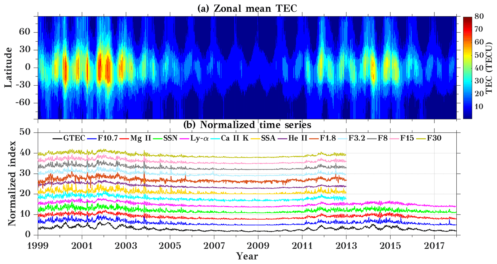
Figure 1Time series of (a) zonal mean TEC and (b) smoothed normalized datasets of GTEC and different solar proxies for the years 1999 to 2017. The curves in (b) are vertically offset by 3 each. x axis labels refer to 1 January of the respective year.
In SC 23, the TEC values at low latitudes reach up to 80 TECU, while during SC 24 TEC was considerably smaller, which confirms that the zonal mean TEC behavior is strongly dependent on the solar activity, as the solar activity was very low during SC 24 compared to SC 23. The amount of free electrons in the ionosphere mainly depends on the photoionization of atomic and molecular neutrals due to solar EUV radiation along with the recombination at different heights and solar zenith angles. The lowest TEC values are observed in the years 2008 and 2009 during the extended solar minimum of SC 23 (Nikutowski et al., 2011). From the zonal mean plot (Fig. 1a), temporal variations are visible, which result from annual and semi-annual variations in the ionosphere. Figure 1b shows the normalized time series of GTEC and 12 solar proxies for the available data in the analyzed time period 1999–2017. Note that Emmert et al. (2017) showed that GTEC values before 2001 are lower than values observed later. This effect should, however, be of minor importance for our analyses below. As the ionosphere response to solar radiation varies for different wavelengths, we used 12 solar proxies based on different measurement techniques and spectral characteristics. Hocke (2008) analyzed GTEC and Mg II index observations and showed that 1 % change in Mg II index results in about 22 % change in GTEC. The time series in Fig. 1 show a similar overall variation during the 11-year solar cycle. The fundamental behavior of solar radiation emission is not identical at all wavelengths and thus for all solar proxies, as the plasma heating and atomic processes are different (Dudok de Wit et al., 2014) but the long-term trends and variations look similar for all the proxies shown here.

Figure 2Long-term diurnal and annual mean TEC distribution during the years 1999 to 2017. The white contour lines indicate the standard deviation based on daily data. The black dashed line represents the magnetic equator.
Figure 2 shows the spatial variation of TEC averaged over the period 1999 to 2017, where the superimposed white contour lines show the standard deviation calculated from the daily TEC data. The magnetic equator is indicated by a dashed black line. A similar analysis has been shown by Guo et al. (2015) using the same TEC dataset within the period 1999 to 2013, finding a comparable spatial distribution. The maximum TEC values are distributed along the equator around ±20∘ and decrease towards the poles. Maximum values of the standard deviation are observed in the low-latitude region with about 15 TECU. The spatial distribution of TEC depends on the ionization of neutrals, transport processes, and recombination, which varies with latitude and longitude.
Note that the T-I system is not only influenced by the solar electromagnetic radiation but also by changing solar energetic particles and geomagnetic conditions due to solar wind variations or coronal mass ejections reaching the Earth (e.g., Abdu, 2016; Tsurutani et al., 2009). The response to solar forcing is higher during solar maximum when the interaction of the solar wind with Earth's upper atmosphere causes ionospheric disturbances at high latitudes along magnetic field lines visible in enhanced TEC values. During solar maxima, the T-I regime can partially be controlled by the solar wind activity superseding the solar radiation impact. However, during periods of low solar activity, the local variability in the ionosphere is also not only regulated by the solar radiation but can be influenced by lower atmospheric forcing (e.g., Forbes et al., 2000; Knížová et al., 2015) and by the solar wind, in particular from coronal holes (e.g., Zurbuchen et al., 2012; Verkhoglyadova et al., 2013).
3.2 Spectra of GTEC and solar proxies
The datasets mentioned above are used to analyze the oscillatory behavior of the T-I system. The periodicities in the solar proxies have been studied by various authors to explore the response of the terrestrial atmosphere and especially the T-I region to solar variability. Here we will investigate and compare the different temporal patterns of GTEC and multiple solar proxies, since proxies may differ in their periodicity depending on the underlying source mechanism.
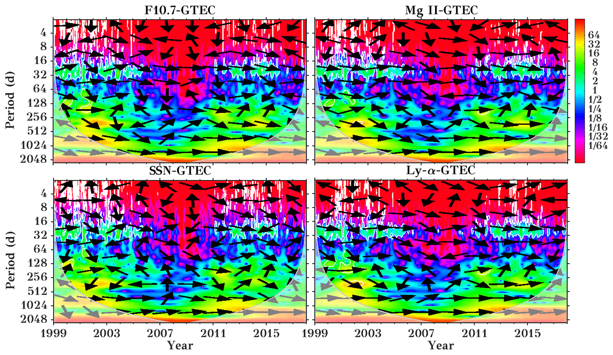
Figure 3Cross-wavelet spectra for GTEC and different solar proxies during the years 1999 to 2017. The thin gray line shows the cone of influence, where a white line surrounds significant values. The arrows indicate the phase relationship, with in-phase and anti-phase relation shown by arrows pointing to the right and left, respectively, while a downward or upward direction means that GTEC is leading or lagging, respectively. x axis labels refer to 1 January of the respective year.
The cross-wavelet technique from Grinsted et al. (2004) was applied, where Morlet wavelets were used as mother functions. The cross-wavelet technique allows common high-power regions between two time series to be indicated. This allows us to determine the dominant correlated oscillations of the ionosphere and important solar proxies. The cross-wavelet analyses of GTEC with four selected solar proxies (F10.7, Mg II, SSN, and Ly-α) are shown in Fig. 3. The most dominant periods observed are in the 16 to 32 d interval visible in all GTEC solar proxy relations during solar maxima. This is, however, not the case during solar minimum when the solar-driven ionospheric variation is lower due to lower solar activity, and the influence of other dynamical processes in the ionosphere (e.g., lower atmospheric forcing) is stronger. Another high-power region is visible in the 128 to 256 d period, representing the semi-annual oscillations in both GTEC and solar parameters. The semi-annual oscillation is mostly dominant during the solar maximum years 2001–2002 and 2011–2012. The black arrows in Fig. 3 indicate the phase relationship between solar proxies and GTEC, with in-phase (anti-phase) relation shown by arrows pointing to the right (left), while a downward (upward) direction means that GTEC is leading (lagging). As expected, in the region of 16 to 32 d GTEC is broadly in phase with the solar proxies, whereas this behavior is not consistent in the semi-annual (128 to 256 d) and annual (256 to 512 d) period ranges. The most dominant joint annual oscillations are observed between GTEC and Ly-α. The annual oscillation can be found mostly during solar maximum.
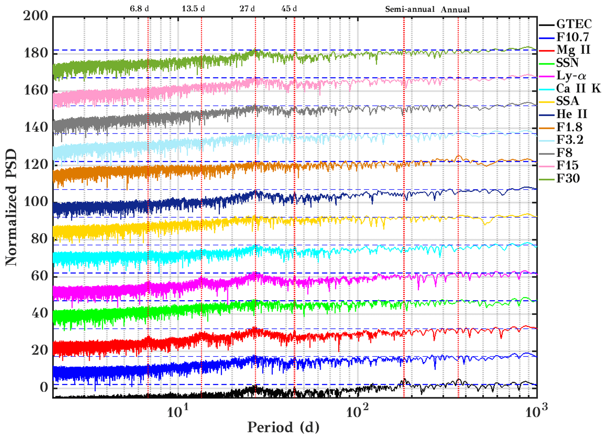
Figure 4Lomb–Scargle periodogram for GTEC and multiple solar proxies with a 95 % confidence line (dashed blue color line). The curves are vertically offset by a factor of 15 each.
To examine the oscillatory behavior of GTEC and solar proxies more precisely, the Lomb–Scargle periodogram (LSP, Lomb, 1976; Scargle, 1982) technique was used. The corresponding spectral analysis is shown in Fig. 4. Here, the power was normalized and converted into a logarithmic scale, and the 95 % confidence level is added to each spectrum as a dashed blue line. The curves have been vertically offset by 15. In this analysis, data from 1999 to 2012–2017 were used. The dominant frequencies observed in GTEC are 27 d, annual, and semi-annual, which is in line with Hocke (2008). Clearly visible in all the solar proxies as well as in GTEC is the mean solar rotation period of about 27 d. Pancheva et al. (1991) showed that the 27 d variation in the lower ionosphere (D region) is often predominantly caused by dynamical forcing (planetary waves), not by direct solar forcing, particularly in winter under low solar activity. However, the D region ionization contributes only weakly to TEC. A 45 d periodicity is observed GTEC, F10.7, Mg II, and SSN. A 45 d periodicity was reported in various solar proxies (Lou et al., 2003; Kilcik et al., 2016, 2018; Chowdhury et al., 2015) using LSP and wavelet analysis. Lou et al. (2003) reported a period of about 42 d in X-Ray solar flares during SC 23. Kilcik et al. (2018) analyzed sunspot counts in flaring and non-flaring active regions for SCs 23 and 24 and observed a 45 d periodicity in flaring active regions. They concluded that a 45 d period is one of the fundamental periods of flaring active regions. A similar periodicity was observed during SC 24 by Chowdhury et al. (2015) in SSA, SSN, and the F10.7 index.
In the Mg II index, which is widely used to represent the solar variability, the dominant periods observed are 27 d, and its second harmonic 13.5 d also described by Hocke (2008). Here the same oscillation is also visible in the Ly-α spectrum. In the F1.8 index, the annual frequency is observed. A semi-annual oscillation is seen in GTEC. This variation is associated with a dynamical effect of the atmosphere (Liu et al., 2006). Note that the wavelet spectra show some periodicity at the half-year timescale for GTEC and F30, but with variable phase so that they extinguish in the periodogram. 128 and 256 d periodicities were reported by various authors (Lou et al., 2003; Kilcik et al., 2014, 2018; Chowdhury et al., 2009). Lou et al. (2003) reported a 259±24 d variation in M5 class X-ray flares during the solar maximum of SC 23. This periodicity may be attributed to non-flaring active regions and developed sunspot groups (Kilcik et al., 2018). Further, Kilcik et al. (2014, 2018) confirmed that the 128 d periodicity is one of the characteristic periodicities of solar flares and also flaring active regions.
3.3 Wavelet cross-correlation
To evaluate the relation between the solar proxies and GTEC, we analyzed the wavelet cross-correlation for the different periods 8 to 16, 16 to 32, 32 to 64, and 64 to 128 d using the wavelet cross-correlation sequence method based on the maximal overlap discrete wavelet transform (MODWT) technique (Percival and Walden, 2000). The MODWT technique is a modified version of the discrete wavelet transform from Mallat (1989).

Figure 5Wavelet cross-correlation sequence estimates for the maximal overlap discrete wavelet transform for GTEC and multiple solar proxies for different timescales (8 to 16, 16 to 32, 32 to 64, and 64 to 128 d). The background color shows the correlation coefficient, and the inserted number shows the delay in days.
In Fig. 5 these cross-correlation coefficients are indicated by the background color, while the inserted numbers show the ionospheric delay in days. The delay is mostly positive, which means that TEC is following the solar proxies. On the 8 to 16 d timescale, maximum correlation is found for He II with a correlation coefficient of about 0.62, and the second maximum correlation is observed for the F15 index, both with a lag of about 1 d. The lowest correlation of about 0.25 is found for the F1.8 index. Compared to the 8 to 16 d period range, the 16 to 32 d period shows a much stronger correlation, with more than about 0.6 for all the proxies. Here a maximum correlation of about 0.9 is observed for the He II and Mg II index, with a GTEC delay of about 1 d. The F30 index and the Ly-α index also shows a strong correlation. The lowest correlation of 0.59 is seen for the daily SSA. A similar result can be observed in the 32 to 64 d period range. Here, maximum correlation is observed again for the He II and Mg II indices, which have a correlation coefficient of 0.9 and a delay of about 2 d. Another particular strong correlation of about 0.8 is observed with Ly-α and Ca II K having a GTEC delay of about 1 and 2 d, respectively. Only a weak correlation of about 0.5 with small GTEC lag time is seen for the daily SSA. The similar behavior in the 16 to 32 and 32 to 64 d intervals is owing to the fact that the 27 d periodicity is only a mean value of the solar differential rotation. It also strongly depends on the lifetime and proper motion of the observed active regions. This results in strong correlations, also observable in the 32 to 64 d interval. In the 64 to 128 d interval, a longer time lag is reached with above 5 d for several proxies. Here the maximum correlation is found for the He II index with about 0.6 and the weakest correlation is seen with about 0.4 for the F1.8 index. Generally, the Mg II and He II proxies show the strongest correlation with GTEC for all period intervals. A strong correlation is also seen for Ly-α and F30, while the weakest correlation is seen for F1.8 and the daily SSA. Figure A1 in the Appendix shows the correlation between solar proxies and GTEC at zero lag at different timescales. Like Fig. 5 it shows strong correlation for Ly-α and F30.
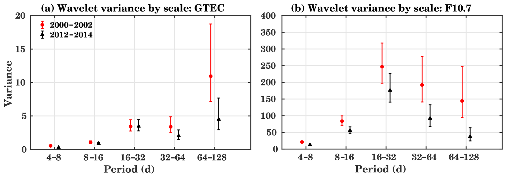
Figure 6Wavelet variance for the maximums of SC 23 (2000–2002, red) and 24 (2012–2014, black) for (a) GTEC and (b) F10.7. Error bars show the 95 % coverage probability of the confidence interval obtained from the “Chi2Eta3” confidence method.
Figure 6 shows the wavelet variance estimated for GTEC and F10.7 using the MODWT technique with the Daubechies 2 (db2) wavelet filter. Here we have selected the time series from the years 2000 to 2002 (maximum of SC 23) and 2012 to 2014 (maximum of SC 24). The red (black) color in the plot represents the SC 23 (SC 24) maximum. In GTEC, maximum variance appears in the 64 to 128 d interval, which is about a quarterly annual oscillation and belongs to the seasonal cycle, during SC 23. The second strongest variance is observed at the 16 to 32 d interval. A generally stronger variance can be observed in SC 23 compared to SC 24 for all the analyzed period intervals. In the case of the F10.7 index, the maximum variance is visible at the 16 to 32 d interval, which here shows a predominant variance for the solar rotation period. As expected, no significant semi-annual cycle is visible. Here again, the observed variance during SC 23 is stronger compared to SC 24.
3.4 Influence of the solar activity on GTEC
This work aims to understand the interaction between solar radiation and the T-I system, especially at the timescale of the solar rotation. To scrutinize the consequence of different solar activity levels on the T-I system for short and intra-annual (including all variability) timescales, we evaluate the running cross-correlation analysis between GTEC and solar proxies as shown in Fig. 7.
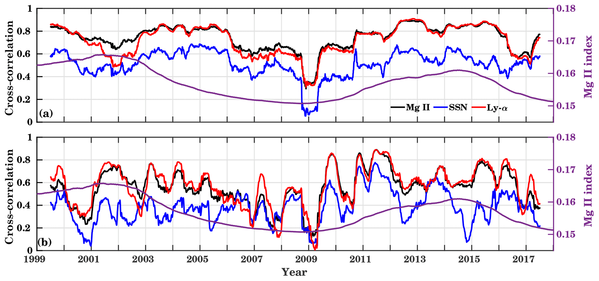
Figure 7Running cross-correlations between GTEC and different solar proxies for (a) short (27 d residual), and (b) intra-annual timescales (original time series). For the short timescale the 27 d residuals have been calculated by removing the 27 d running mean from the original datasets. A 365 d running window is used to calculate the correlation. The second y axis shows 365 d (a and b) running mean time series of Mg II index. Here Mg II, SSN, and Ly-α are marked by black, blue, and red colors, respectively.
Figure 7a shows the running correlation for the short timescale. To calculate the short-term variation at the solar rotation period, the 27 d residual has been calculated by subtracting the 27 d running average values from corresponding datasets of GTEC and solar proxies (Mg II, SSN, and Ly-α). The running correlation is calculated using the filtered time series at the solar rotation period by using a 365 d running window. The 365 d running mean Mg II index is added to show the overall solar activity in Fig. 7a and b. The correlation is likely to vary with respect to solar activity. Lower correlation is observed during low solar activity. A similar kind of analysis was shown by Chen et al. (2012).
Furthermore, to understand the relation between GTEC and solar proxies at longer timescales, we calculate the cross-correlation between the annual means. The maximum correlation observed is about 0.93 (figure not shown) between the solar proxies and GTEC. Hence in comparison to short timescales variations, solar proxies are strongly correlated with GTEC.
Figure 7b shows correlation at the intra-annual timescale, which includes all the variations, i.e., seasonal, daily, and solar rotation. Here, a 365 d running window is used to calculate the running correlations based on unfiltered data. The correlation with all the solar proxies is smallest during the extended low solar activity phase during the solar minimum in 2008–2009. All solar proxies show similar behavior during low activity conditions: while the temporal variation of the correlation coefficient for Mg II and Ly-α is largely similar, the SSN (blue curve) shows significantly different behavior. The strongest correlation is observed during the rising part of solar cycle 24. In comparison to all the other solar proxies, Mg II and Ly-α show a stronger correlation with GTEC, while the lowest correlation is given for SSN at short and intra-annual timescales.
Solar EUV variations can be well described by the solar proxies (e.g., F10.7, SSN) at the 11-year solar cycle variations but they show weak correlation at short timescales (daily, 27 d solar rotation period) (e.g., Chen et al., 2012; Floyd et al., 2005) as shown in Fig. 7. At longer timescales, solar EUV and solar proxies are mainly controlled by solar magnetic activity. But at short timescales, these parameters vary differently as they originate from different excitation mechanisms in the solar surface (e.g., Chen et al., 2012; Lean et al., 2001).
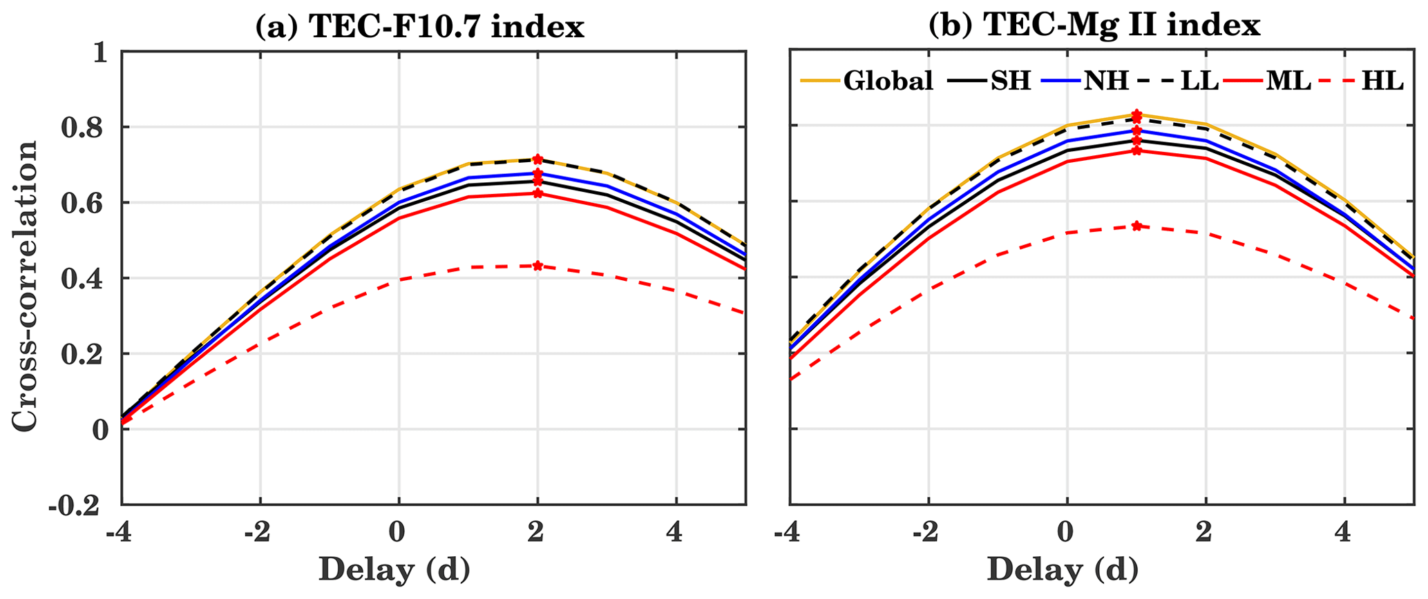
Figure 8Cross-correlation coefficients and time delays between the global, Northern Hemisphere (NH), and Southern Hemisphere (SH) as well as low-latitude (LL, ±30∘), midlatitude (ML, ± (30–60∘)), and high-latitude (HL, ± (60–90∘)) TEC with (a) F10.7 and (b) Mg II index during the years 1999 to 2017 for a different lag. A positive lag means that solar flux variations are heading TEC ones. The maximum correlation is indicated by a red star.
Figure 8 shows the cross-correlation analysis of (a) F10.7 and (b) Mg II with the global, Northern Hemisphere (NH), Southern Hemisphere (SH), low-latitude (LL, ±30∘), midlatitude (ML, ± (30–60∘)), and high-latitude (HL, ± (60–90∘)) mean TEC. Generally, the correlation coefficients and the lag for the global, NH, SH, LL, and ML are very close to each other. The maximum correlation is found for GTEC and LL TEC with correlation coefficients of about 0.7 (F10.7) and 0.82 (Mg II) for a time delay of about 2 and 1 d, respectively. Generally, GTEC variability is mainly determined by the LL electron content, so that it is expected that the correlation coefficients for GTEC and LL are similar. The weakest correlation is observed for HL with a maximum correlation coefficient of 0.42 (F10.7) and 0.53 (Mg II) and a corresponding ionosphere response time of about 2 and 1 d, respectively (marked with a red star). NH and SH are comparable with slightly smaller correlations for SH. There is a weaker correlation for ML compared to LL, but the difference is not as large as the one for HL. Running correlations at intra-annual timescales, similar to Fig. 7, are shown in Fig. A6 in the Appendix.
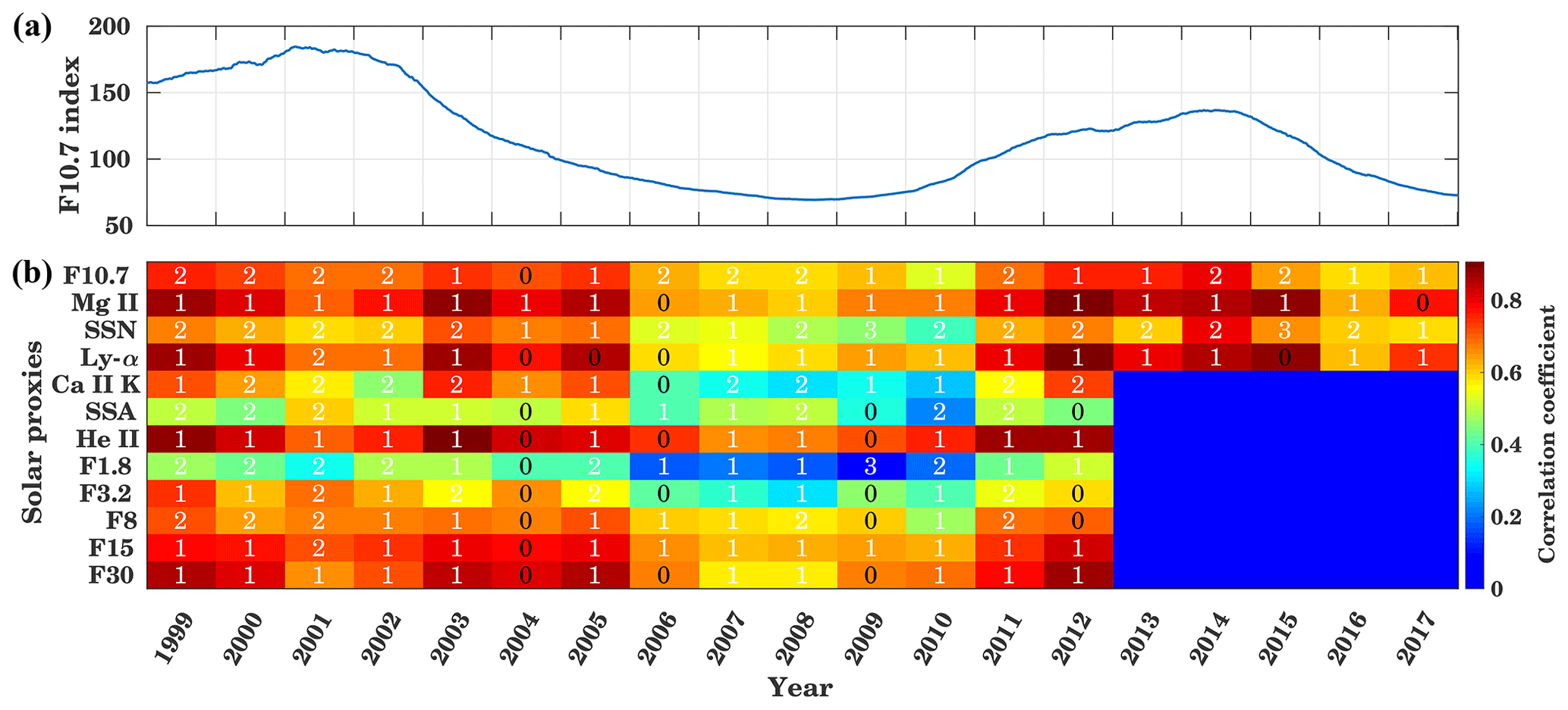
Figure 9In panel (a), the 365 d running mean time series of F10.7 is shown. Panel (b) displays yearly cross-correlations and time delays between GTEC and different solar proxies for the years 1999 to 2017 at the timescale of 16 to 32 d. The background colors give the maximum correlation coefficient, and the inserted numbers show the delay in days corresponding to maximum correlation.
Figure 9 shows the cross-correlation analysis between GTEC and solar proxies separately for each year at the timescale of 16 to 32 d. To calculate the wavelet cross-correlation, the data are filtered for different timescales using the MODWT. Figure 9a shows the 365 d running mean F10.7. The delay is given as numbers inserted on the color-coded cross-correlation for the different solar proxies and time periods. As in Fig. 7, the overall trend shows that the correlation is weak during solar minimum and strong during high solar activity periods. The time delay ranges between 0 and 3 d for all solar proxies, but without obvious regularity with respect to the proxies or the time. As in Fig. 5, a generally strong correlation is found for He II and Mg II, while daily SSA and F1.8 indices show the weakest correlation. During the years of low solar activity 2007–2010, an especially weak correlation is visible for F3.2, F1.8, and Ca II K. The maximum F10.7 index is observed during 2001 with about 181 sfu. During the high solar activity years from 1999 to 2003 and from 2012 to 2014 a strong correlation of about 0.85 is observed for Mg II, He II, F30 (1999–2003, 2012), and Ly-α except for 2001, when the maximum annual mean F10.7 index is observed. During the maximum of SC 23, the cross-correlation between Mg II, He II, Ly-α, F3.2, F15, and GTEC is about 0.7 with a delay of about 1–2 d. A weak correlation is observed for F1.8 and Ca II K. During low solar activity (years 2006–2010, 2016) when the average F10.7 index is below 75 sfu, a stronger correlation is observed between He II and Mg II and GTEC, with a correlation coefficient of more than 0.6. Only a weak correlation during low solar activity is observed for F1.8, Ca II K, F3.2, and daily SSA. During moderate solar activity years (2004–2005, 2011, 2015), when the average F10.7 index is about 90–120 sfu, Mg II, He II, F30, and Ly-α show stronger correlation with GTEC with a delay of about 1 d. In summary, during low solar activity, most of the solar proxies show a weak correlation with GTEC but strong correlation is found for high solar activity. In comparison to other solar proxies, F1.8 and SSA are weakly correlated with GTEC. Figure A2 in the Appendix shows the correlation at a 16 to 32 d timescale between solar proxies and GTEC at zero lag. It shows a similar correlation to Fig. 9. In comparison to the 16 to 32 d timescales, we further analyzed the cross-correlation and delay at 32 to 64 d timescales (Fig. A3 in the Appendix).
In summary, the most suitable proxy to represent the solar activity at the timescale of 16 to 32 and 32 to 64 d during low, moderate, and high solar activity is He II. The Mg II index, Ly-α, and F30 also show a strong correlation with GTEC, but there are some differences in correlation during solar maximum and minimum years, as the behavior of proxies is not always the same. The F1.8 and daily SSA cannot adequately represent the solar activity at the solar rotation (16 to 32 d) timescale. As discussed above, solar proxies are more weakly correlated at shorter timescales than at longer timescales.
3.5 Spatial distribution of the ionospheric response time
Here we investigate the inter-annual spatial variability of the ionospheric response to solar variations. Figure 10 shows correlation and time lag between TEC and Mg II globally for a TEC map resolution of 2.5∘ in latitude and 5∘ in longitude. The left column shows yearly zonal means, while the right column shows 1999 to 2017 means with longitudinal resolution. The contour maps in Fig. 10a (b) show the cross-correlation (time delay) where the inserted contour lines represent the standard deviation.
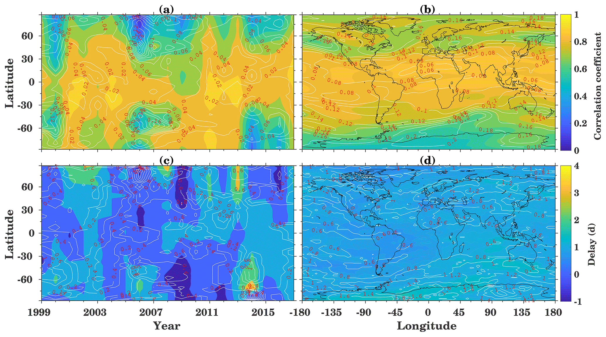
Figure 10(a, c) Zonal mean and (b, d) long-term mean correlation coefficients (a, b) and time delay (c, d) between TEC and Mg II index for the years 1999 to 2017. The white contour lines indicate the respective standard deviations.
Maximum correlation of about 0.9 is observed during high solar activity years at low latitudes. Figure 10a, b show that the correlation decreases from low to high latitudes. In the NH, the correlation is the weakest south of the auroral oval, probably due to the fact that particle precipitation also changes with solar wind dynamics. Figure 10c shows the zonal mean time delay for the year 1999 to 2017, which is about 1 d in the low and middle latitudes. The delay generally increases towards high latitudes with a few exceptions occurring during low solar activity. There is a tendency that during high solar activity, the delay is increased slightly at low latitudes, but strongly (up to 3 d) in the high-latitude region. A negative delay is observed during low solar activity, presumably associated with the meteorological effects as suggested by Ren et al. (2018). Another possible reason is ionospheric saturation, which might reduce the transport process during high solar activity due to lower recombination rates. Transport is one of the most critical parameters that control the behavior of the ionosphere. These results suggest that interannual variability depends not only on the solar activity but also on several other physical processes such as geomagnetic activity (Rich et al., 2003) and local ionospheric parameters such as neutral wind and lower atmospheric forcing through the vertical coupling. Lee et al. (2012) analyzed electron density measurements from CHAMP and GRACE along with Global Ionosphere Maps (GIM) TEC maps in relation to the F10.7 index and showed the spatial distribution of delay and correlation coefficient during the years 2003 to 2007. They found a strong (weak) correlation between GIM TEC and F10.7 in the midlatitude (high-latitude) region, with a time delay of about 1–2 (2–4) d which qualitatively confirms our results. Figure 10d shows the spatial distribution of the time delay, where an overall time delay of about 1 d with a standard deviation of less than 1 d is visible. The time delay is longer for the high-latitude region, whereas the cross-correlation is weaker, as can be seen in Fig. 10b. In this region, the standard deviation is more than 1 d.
3.6 EOF analysis of ionospheric TEC
Ionospheric TEC is varying diurnally, daily, and seasonally, on a decadal scale, as well as in latitude and longitude. To examine the spatial variability of TEC, we applied the principal component (PC) analysis for signal decomposition (Preisendorfer, 1988; Björnsson and Venegas, 1997) using EOFs, which decompose data into orthogonal modes of variability caused by solar and geomagnetic activity. The method is used to decompose the spatial–temporal field of TEC (time, longitude, latitude) into EOF components. To this end, we first calculate the data covariance matrix by using the TEC datasets, followed by finding the eigenvalues and corresponding eigenvectors (the EOFs). The explained variance of the kth EOF is the corresponding eigenvalue divided by the sum of all eigenvalues. The PC is found by projecting the TEC anomalies onto the EOF. This method has been used to represent the variability in the T-I system and for T-I modeling (e.g., Zhao et al., 2005; Matsuo et al., 2012; Ercha et al., 2012; Anderson and Hawkins, 2016; Talaat and Zhu, 2016).
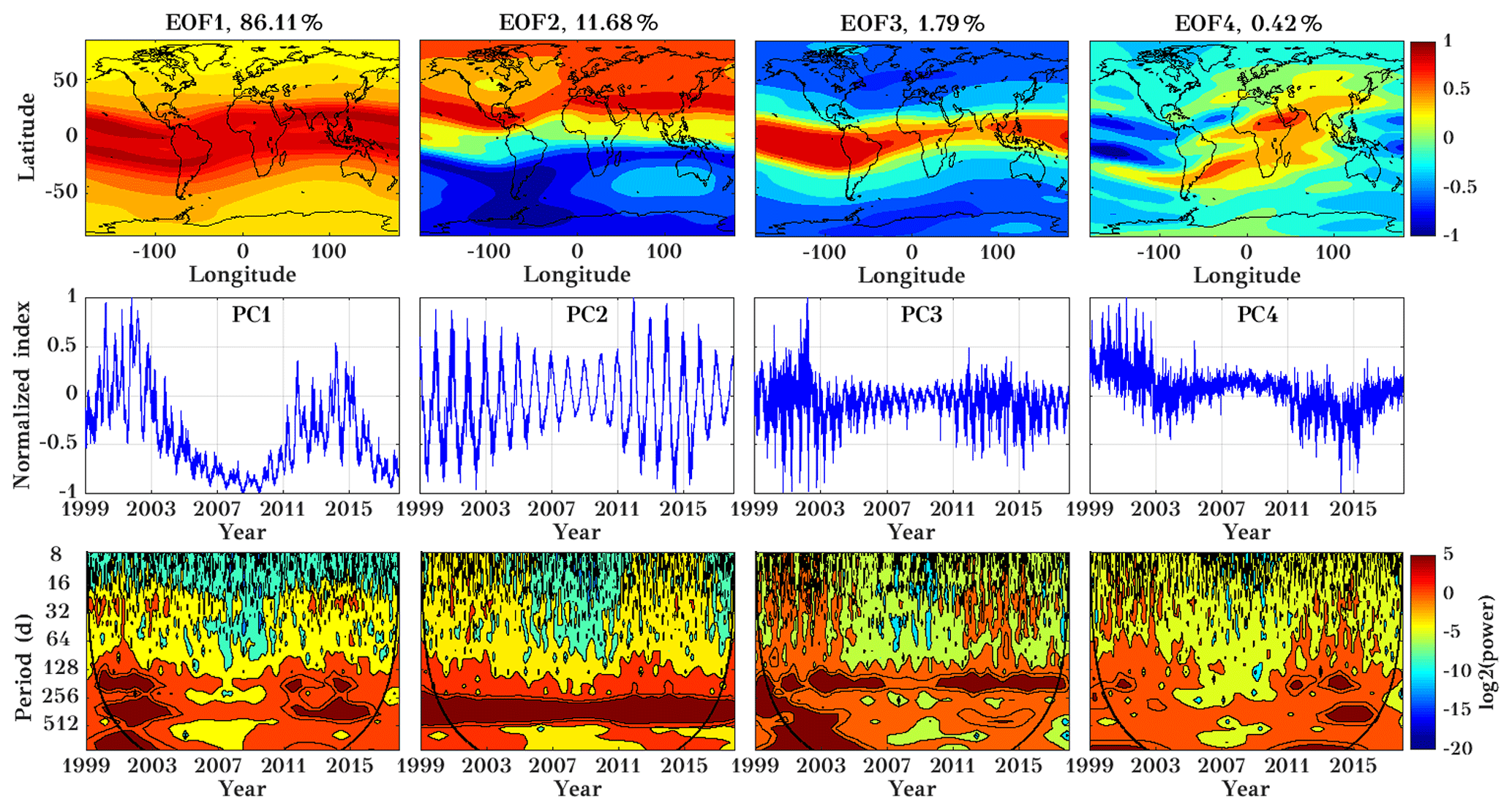
Figure 11The first four EOFs (top row) of normalized TEC during the years 1999 to 2017, corresponding principal components (middle row), and their corresponding wavelet transform (bottom row, wavelet power in log2 scale). Please note that EOFs are dimensionless.
We analyzed the TEC datasets in a spatial grid of 71∘ × 72∘ (latitude and longitude) and a temporal length of 6940 d. Figure 11 shows the first four EOF maps in the upper panels followed by the PCs (middle panels) and the corresponding wavelet spectra (lower panels). The first three EOFs are similar to those presented by Talaat and Zhu (2016). The first EOF component explains approximately 86 % of the variance. A high variability in the low-latitude region and a smaller one at higher latitudes is shown. EOF1 shows the spatial distribution of TEC variance in general and is positive everywhere. This indicates a joint in-phase variability of the entire ionosphere, which is larger at low latitudes. Consequently, as is shown in the middle panel of Fig. 11, its temporal amplitude varies from positive to negative following the solar activity and the annual and semiannual cycle. In the lower panel of Fig. 11, the wavelet analyses for the EOFs are shown. To get clear periodicity from the wavelet, we have used log2 of the power. Negative (positive) values indicate low (high) power. The wavelet analysis of EOF1 shows a 27 d periodicity associated with the solar rotation period. Annual and semi-annual oscillations are observed, especially during the high solar activity years. The EOF2 captures 11 % of the total variability and demonstrates a hemispheric asymmetry. The corresponding PC and wavelet analysis show a strong annual variability connected with seasonal variability and larger TEC during winter.
EOF3 captures about 1.79 % of the total variability. EOF3 might be associated with non-solar effects and fine structures of the solar activity response, which is not captured by the first EOF as suggested by Talaat and Zhu (2016). Note that EOF3 essentially shows a semi-annual and a relatively strong 27 d variability. EOF4 contributes with only 0.4 % of the total estimated variability. Its shape is strongly non-zonal and reflects variations in longitudinal differences of the equatorial ionization anomaly. In the wavelet analysis, weak semi-annual and annual oscillations are visible. Note that the PC4 displays a possible long-term trend, which may indicate an effect of the secular change of the main magnetic field of the Earth. The oscillating structure of the EOF4 over the Atlantic resembles the results from numerical simulations by Cnossen and Richmond (2013).
In summary, the first two components capture almost 98 % of the TEC variance, while the third and fourth components only contribute about 2 %. This is similar to results of Zhao et al. (2005), Anderson and Hawkins (2016), and Talaat and Zhu (2016), who reported that more than 95 % of the variance is explained by the first three EOFs.
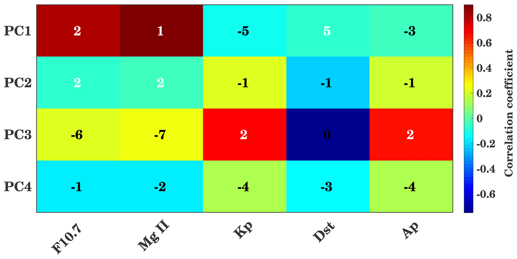
Figure 12Correlation coefficients and time lag between the PCs and solar and geomagnetic proxies. Background colors show the maximum correlation coefficients, and the inserted numbers show the delay in days corresponding to maximum correlation.
In order to check the relation between solar proxies and geomagnetic parameters (daily Kp, Dst, and Ap indices) with PCs corresponding to EOFs, the wavelet cross-correlation and delay are shown in Fig. 12. In Fig. 12 the color indicates the maximum correlation coefficient, and the numerical values indicate the corresponding time delay in days. A strong correlation between PC1 and Mg II (F10.7) is observed with a coefficient of about 0.87 (0.8) and a time delay of 1 d (2 d). This represents the strong correlation between global TEC and solar variability as PC1 is associated with solar variability. The geomagnetic parameters are generally more loosely connected with ionospheric variability, indicating the relatively fast ionospheric storm reaction compared to the longer-lasting equatorial magnetic field depletion. PC3 shows a relatively strong correlation with the geomagnetic parameters, which indicates that this component (apart from the remaining part of solar variability not included in EOF1) captures the geomagnetic activity effect on TEC. Here the Kp and Ap indices show a positive correlation of about 0.6 with a delay of about 2 d. In comparison to this, a negative correlation of about 0.7 is observed in the Dst. Figure A4 in the Appendix shows the correlation between PCs and solar and geomagnetic proxies at zero lag. Furthermore, running correlations at interannual timescales, similar to Fig. 7 are shown in Fig. A7 in the Appendix using PCs and solar and geomagnetic parameters.

Figure 13Spatial distribution map of first four EOFs (upper panels) of IGS TEC during the years 1999 to 2017, and their corresponding wavelet transform (lower panels, wavelet power in log2 scale) using a 25–35 d filtered dataset. The EOFs are dimensionless.
To assess the variability on the timescale of the solar rotation period, we filtered the GTEC time series in a period range of 25 to 35 d using a digital bandpass filter. The filtered time series is then used to compute EOFs. Figure 13 shows the first four EOF components in the upper row and their corresponding wavelet transforms in the lower row. The first component captures almost 85.50 % of total variability, and it seems to be associated with solar activity. EOF1 shows high variability in the equatorial region. EOF2 captures 8.91 % of variability, and it is partly associated with hemispheric variability. EOF3 captures the variability of 4.92 %, which is not captured in the EOF2 component (in particular the hemispheric asymmetry). EOF2 does not show a clear hemispheric signal anymore, while EOF3 now does. The lower panels show the corresponding wavelet spectra of PCs. Wavelet analysis clearly shows the expected periodicity in the 16 to 32 d period in all the PCs, with a response to the 11-year solar cycle.
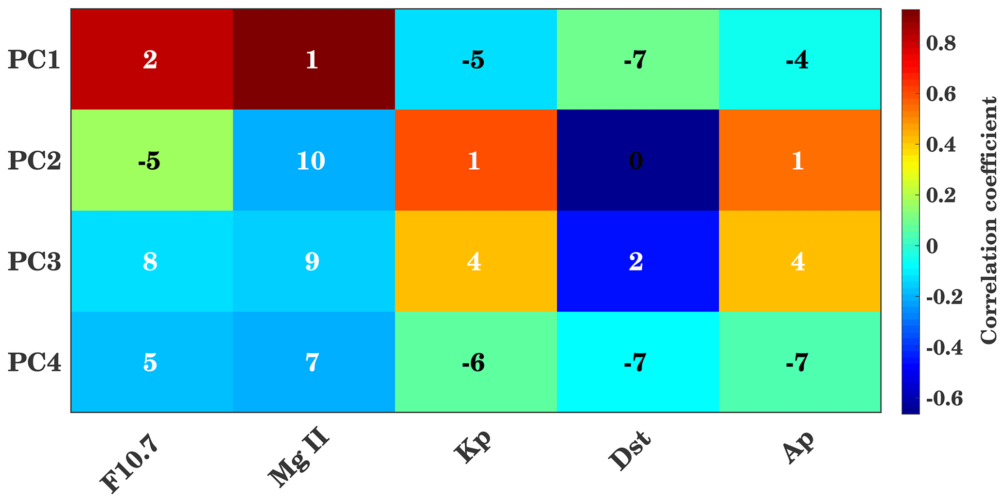
Figure 14Maximum correlation coefficients and the time lag between the PCs and solar and magnetic proxies for the 25–35 d interval. Background colors show the maximum correlation coefficients, and the inserted numbers show the delay in days corresponding to maximum correlation.
Furthermore, wavelet cross-correlation analysis has been performed to understand the relation between solar proxies and geomagnetic parameters (with PCs corresponding to EOFs of the filtered data, as shown in Fig. 13) and shown in Fig. 14 (Fig. A5 in the Appendix for zero lag). It shows a similar kind of result to in Fig. 12 in the case of PC1. PC2 and PC3 are associated with geomagnetic activity. As compared to Fig. 12, PC2 shows strong correlation with magnetic indices. So, the distribution of variance is different here. This is because the coupled low-latitude–high-latitude magnetically forced variability, which is mainly represented by PC3 in the case of unfiltered data, is now distributed among PC2 and PC3 for the solar rotation period.
We have investigated the long-term ionospheric response during different solar activities, timescales, and spatial variations using 12 solar proxies (F10.7, F1.8, F3.2, F8, F15, F30, He II, Mg II index, Ly-α, Ca II K, daily SSA, and SSN) and 18 years (1999–2017) of IGS TEC data. The cross-wavelet and LSP methods were used to examine the oscillatory behavior. The cross-wavelet analysis represents the 16 to 32 d period in all the solar proxies and GTEC. The maximum correlation with GTEC is observed between the He II index, Mg II index, and F30 in the period range of 16 to 32 d along with a time delay of about 1 d. Wavelet variance estimation suggests that GTEC variance is high for the 64 to 128 d interval followed by 16 to 32 d, while the F10.7 index is showing high variance for the 16 to 32 d interval.
Interannual variation of the cross-correlation analysis suggests that the correlation is varying with the solar activity. The most suitable proxy to represent the solar activity at the timescales of 16 to 32 and 32 to 64 d during low, middle, and high solar activity is He II. The Mg II index, Ly-α, and F30 may be placed at the second as these indices show a strong correlation with GTEC, but with some differences between solar maximum and minimum. The F1.8 and daily SSA poorly represent the solar activity effect on TEC. The spatial distribution of cross-correlation and time was estimated using the Mg II index. The results show significant temporal and spatial variations. Stronger correlation is observed near the equatorial region with a time delay of about 1–2 d. The magnetospheric inputs probably strongly influence both high- and low-latitude regions, but with a different sign.
TEC datasets also have been decomposed using EOFs along with the principal component analysis method to signify the spatial and temporal variation. The first EOF component captures more than 86 % of the variability, and the first three EOF components explain 99 % of the variance. EOF analysis suggests that the first component is associated with the solar flux and the third EOF component captures the geomagnetic activity as well as the remaining part of EOF1. EOF2 captures 11 % of the total variability and demonstrates the hemispheric asymmetry.
IGS TEC data are provided via NASA through http://cddis.nasa.gov/Data_and_Derived_Products/GNSS/ (last access: 15 August 2018) (CDDIS, 2018). Daily F10.7 index can be downloaded from http://lasp.colorado.edu/lisird/data/noaa_radio_flux/ (last access: 15 August 2018) (LASP, 2018). Mg II index data are provided by IUP at http://www.iup.uni-bremen.de/UVSAT/Datasets/mgii (last access: 15 August 2018) (IUP, 2018). Solar proxies F30, F15, F8, F3.2, F1.8, Ca II K index, and daily SSA are available from the SOLID database (http://projects.pmodwrc.ch/solid/, last access: 15 August 2018) (SOLID, 2018). The SSN, Ly-α, Kp, Dst, and Ap indices are provided by NASA's Goddard Space Flight Center through https://omniweb.gsfc.nasa.gov (last access: 15 August 2018) (OMNIWeb, 2018).
Additional figures are shown in order to complete the presentation. Figure A1 is similar to Fig. 5 but shows the correlation between solar proxies and GTEC at zero lag at different timescales. Figure A2 shows the correlation at 16 to 32 d timescale between solar proxies and GTEC, similar to Fig. 9, but again at zero lag. Figure A3 is similar to Fig. 9 but shows the cross-correlation and delay at the timescale of 32 to 64 d. Figure A4 is similar to Fig. 12 and shows the correlation between PCs and solar and geomagnetic proxies, but at zero lag, while Fig. A5 shows the same for the 25–35 d interval. Running correlations at the intra-annual timescales, similar to Fig. 7 but also for different latitude ranges, are shown in Fig. A6. Figure A7 shows running cross-correlations between the PCs and different solar proxies and geomagnetic activity parameters.
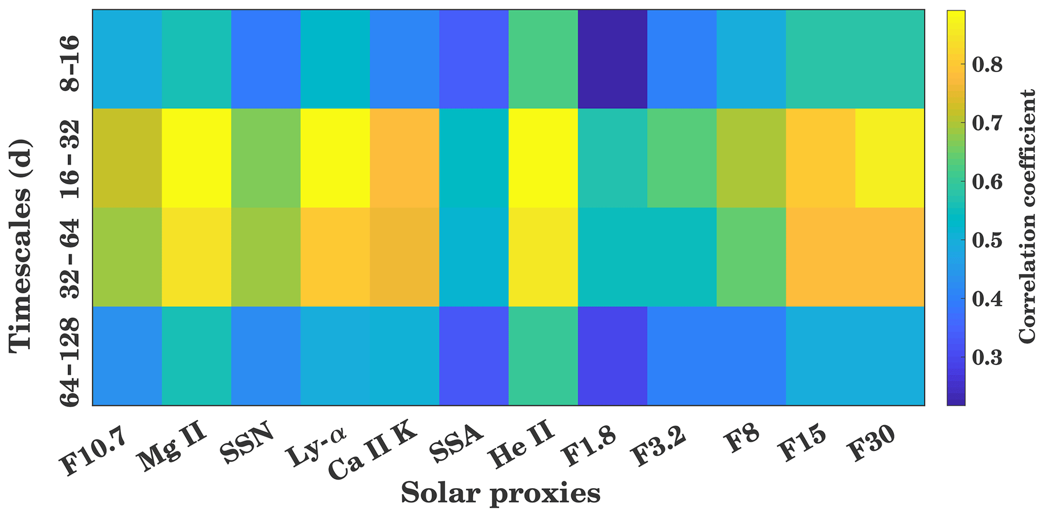
Figure A1Wavelet cross-correlation sequence estimates for the maximal overlap discrete wavelet transform for GTEC and multiple solar proxies for different timescales (8 to 16, 16 to 32, 32 to 64, and 64 to 128 d). The colors represent the correlation coefficient at lag 0.

Figure A2Correlation coefficient between GTEC and different solar proxies for the years 1999 to 2017 at the timescale of 16 to 32 d at lag 0.
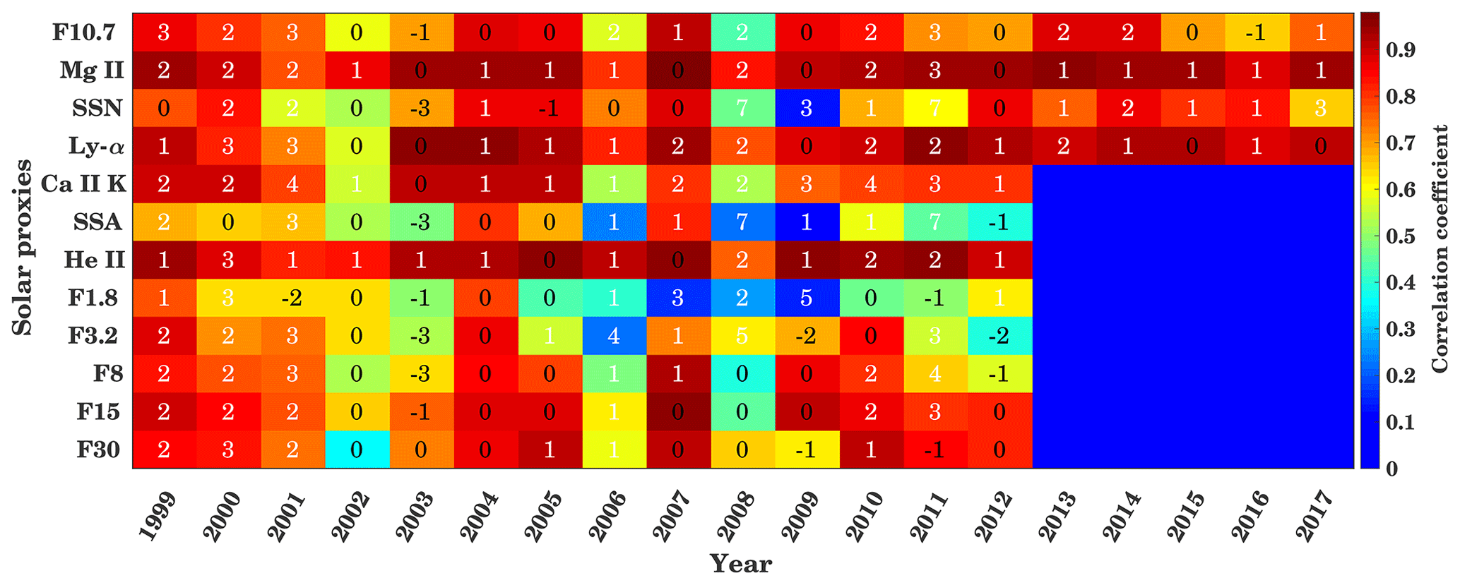
Figure A3Cross-correlation and time delay between GTEC and different solar proxies for the years 1999 to 2017 at the timescale of 32 to 64 d. Background colors show the maximum correlation coefficients, and the inserted numbers show the delay in days corresponding to maximum correlation.
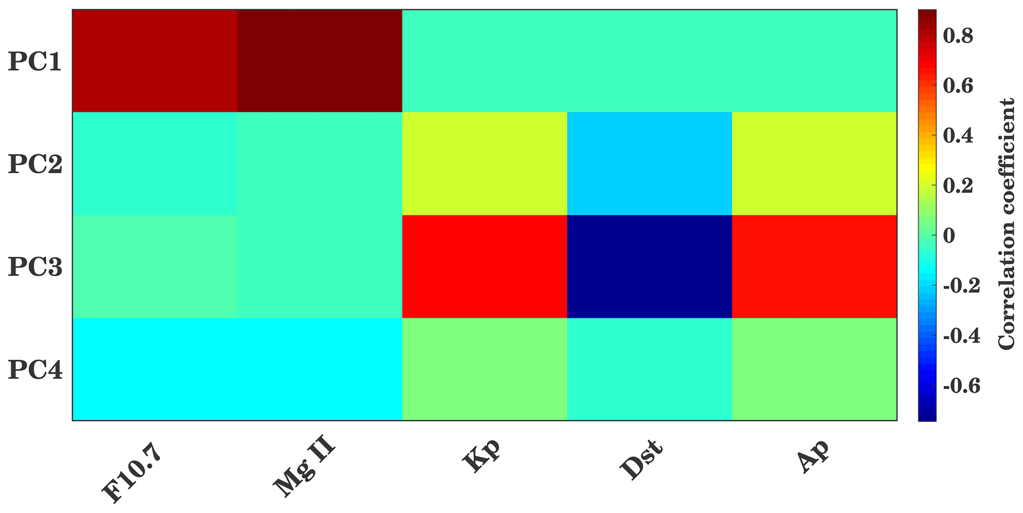
Figure A4Correlation coefficients between the PCs and solar and geomagnetic proxies at lag 0.
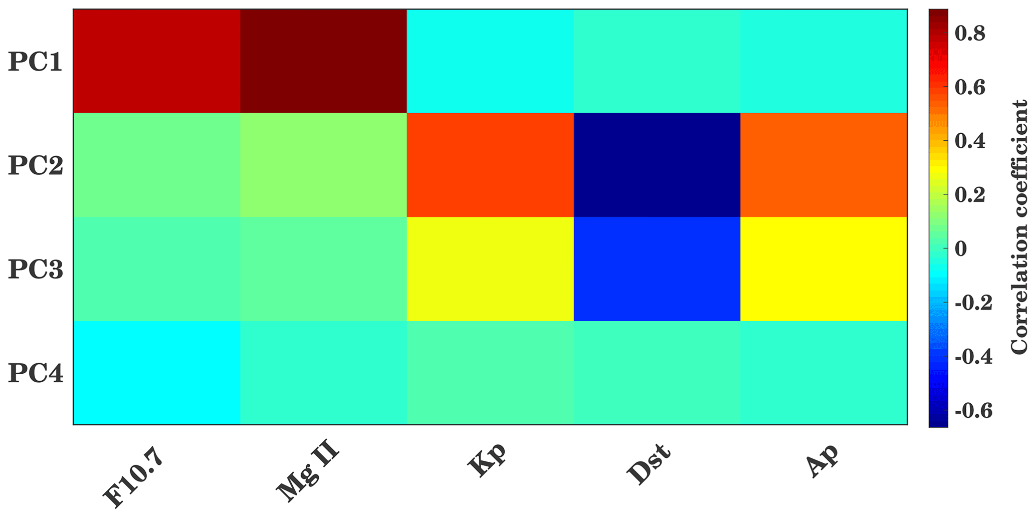
Figure A5Correlation coefficients between the PCs and solar and magnetic proxies for the 25–35 d interval for zero lag.
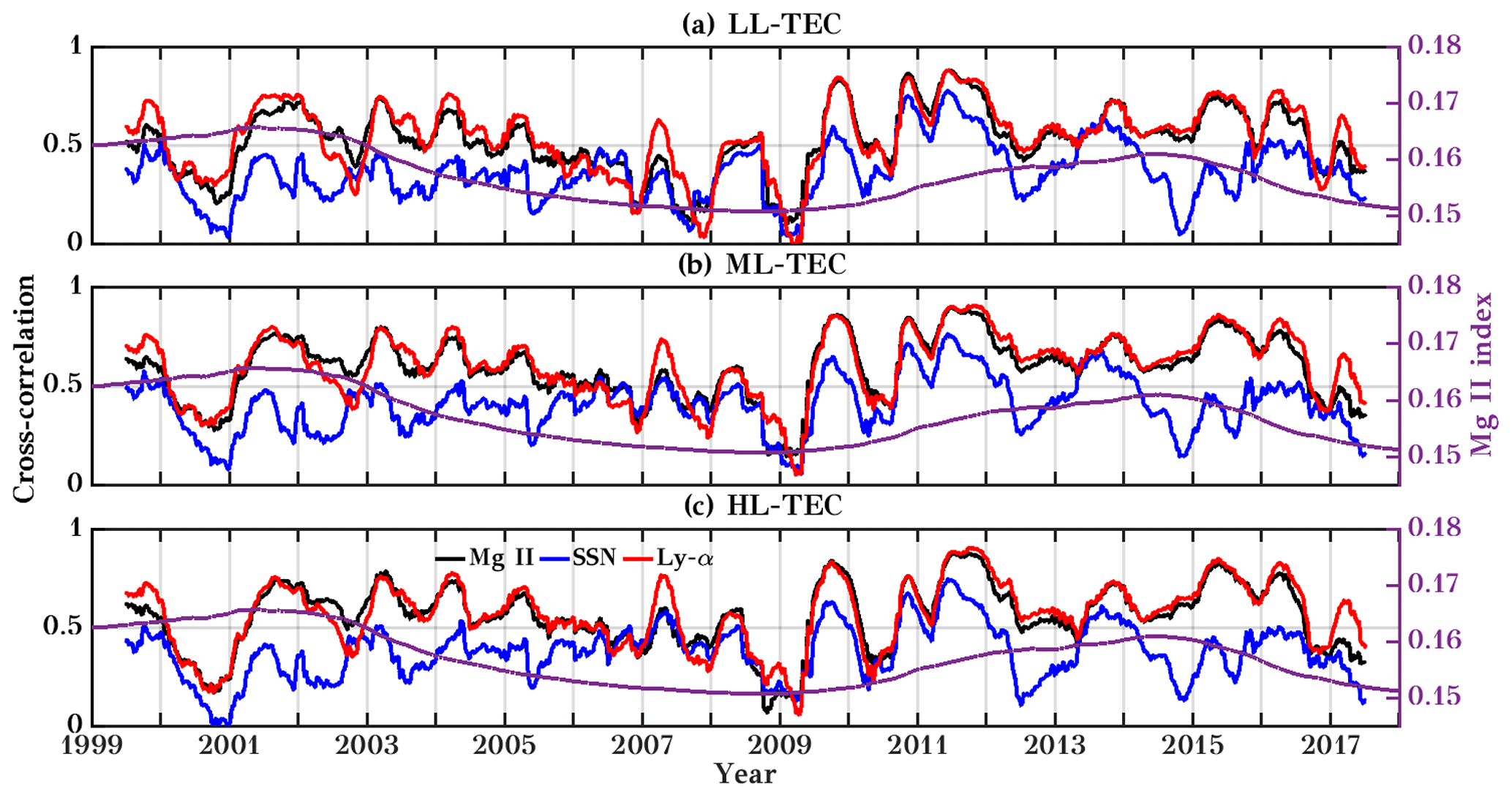
Figure A6Running cross-correlation between the TEC and different solar proxies using a 365 d running window for LL, ML, and HL. The second y axis shows the 365 d running mean time series of the Mg II index. Here Mg II, SSN, and Ly-α are marked by black, blue, and red colors, respectively. Correlation coefficients between the PCs and solar and geomagnetic proxies at lag 0.

Figure A7Running cross-correlation between the PCs and different solar proxies and geomagnetic activity parameters using a 365 d running window. The second y axis shows the 365 d running mean time series of the Mg II index. Here F10.7, Mg II, Kp, Dst, and Ap are marked by black, blue, red, green, and magenta colors, respectively.
CJ, RV, and JB designed the study. RV analyzed the data. RV drafted the first version of the paper. All authors discussed the results and provided critical feedback and contributed to the final version of the paper.
Christoph Jacobi is one of the Editors-in-Chief of Annales Geophysicae. The authors declare that they have no conflict of interest.
This article is part of the special issue “Vertical coupling in the atmosphere–ionosphere system”. It is a result of the 7th Vertical Coupling workshop, Potsdam, Germany, 2–6 July 2018.
We kindly acknowledge NASA for providing the IGS TEC data (NASA), through ftp://cddis.gsfc.nasa.gov/gnss/products/ionex/ (CDDIS, 2018), and the daily F10.7 index (NOAA); Mg II data (IUP); solar proxies F30, F15, F8, F3.2, and F1.8; Ca II K index; daily SSA (SOLID database) and SSN; and Ly-α, Kp, Dst, and Ap indices (NASA's Goddard Space Flight Center). The study has been supported by Deutsche Forschungsgemeinschaft (DFG) through grant nos. JA 836/33-1 and BE 5789/2-1.
This research has been supported by the Deutsche Forschungsgemeinschaft (DFG) (grant nos. JA 836/33-1 and BE 5789/2-1).
This paper was edited by Erdal Yiğit and reviewed by Ana G. Elias and two anonymous referees.
Abdu, M. A.: Electrodynamics of ionospheric weather over low latitudes, Geosci. Lett., 3, 11, https://doi.org/10.1186/s40562-016-0043-6, 2016. a
Afraimovich, E. L., Astafyeva, E. I., Oinats, A. V., Yasukevich, Yu. V., and Zhivetiev, I. V.: Global electron content: a new conception to track solar activity, Ann. Geophys., 26, 335–344, https://doi.org/10.5194/angeo-26-335-2008, 2008. a, b
Anderson, P. C. and Hawkins, J. M.: Topside ionospheric response to solar EUV variability, J. Geophys. Res., 121, 1518–1529, https://doi.org/10.1002/2015ja021202, 2016. a, b
BenMoussa, A., Gissot, S., Schühle, U., Zanna, G. D., Auchère, F., Mekaoui, S., Jones, A. R., Walton, D., Eyles, C. J., Thuillier, G., Seaton, D., Dammasch, I. E., Cessateur, G., Meftah, M., Andretta, V., Berghmans, D., Bewsher, D., Bolsée, D., Bradley, L., Brown, D. S., Chamberlin, P. C., Dewitte, S., Didkovsky, L. V., Dominique, M., Eparvier, F. G., Foujols, T., Gillotay, D., Giordanengo, B., Halain, J. P., Hock, R. A., Irbah, A., Jeppesen, C., Judge, D. L., Kretzschmar, M., McMullin, D. R., Nicula, B., Schmutz, W., Ucker, G., Wieman, S., Woodraska, D., and Woods, T. N.: On-Orbit Degradation of Solar Instruments, Sol. Phys., 288, 389–434, https://doi.org/10.1007/s11207-013-0290-z, 2013. a
Björnsson, H. and Venegas, S.: A manual for EOF and SVD analyses of climatic data, CCGCR Report, 97, 112–134, 1997. a
CDDIS: GNSS Atmospheric Products, available at: http://cddis.nasa.gov/Data_and_Derived_Products/GNSS/atmospheric_products.html, last accessed: 15 August 2018. a, b, c
Chen, Y., Liu, L., and Wan, W.: The discrepancy in solar EUV-proxy correlations on solar cycle and solar rotation timescales and its manifestation in the ionosphere, J. Geophys. Res., 117, A03313, https://doi.org/10.1029/2011ja017224, 2012. a, b, c, d
Chowdhury, P., Khan, M., and Ray, P. C.: Intermediate-term periodicities in sunspot areas during solar cycles 22 and 23, Mon. Not. Roy. Astron. Soc., 392, 1159–1180, https://doi.org/10.1111/j.1365-2966.2008.14117.x, 2009. a
Chowdhury, P., Choudhary, D. P., Gosain, S., and Moon, Y.-J.: Short-term periodicities in interplanetary, geomagnetic and solar phenomena during solar cycle 24, Astrophys. Space Sci., 356, 7–18, https://doi.org/10.1007/s10509-014-2188-0, 2015. a, b
Cnossen, I. and Richmond, A. D.: Changes in the Earth's magnetic field over the past century: Effects on the ionosphere-thermosphere system and solar quiet (Sq) magnetic variation, J. Geophys. Res., 118, 849–858, https://doi.org/10.1029/2012ja018447, 2013. a
Dewolfe, A. W., Wilson, A., Lindholm, D. M., Pankratz, C. K., Snow, M. A., and Woods, T. N.: Solar Irradiance Data Products at the LASP Interactive Solar Irradiance Datacenter (LISIRD), AGU Fall Meeting Abstracts, GC21B-0881, San Francisco, California, 13–17 December 2010. a
Dudok de Wit, T.: A method for filling gaps in solar irradiance and solar proxy data, Astron. Astrophys., 533, A29, https://doi.org/10.1051/0004-6361/201117024, 2011. a
Dudok de Wit, T., Bruinsma, S., and Shibasaki, K.: Synoptic radio observations as proxies for upper atmosphere modelling, J. Space Weather Space Clim., 4, A06, https://doi.org/10.1051/swsc/2014003, 2014. a, b
Emmert, J. T., Mannucci, A. J., McDonald, S. E., and Vergados, P.: Attribution of interminimum changes in global and hemispheric total electron content, J. Geophys. Res., 122, 2424–2439, https://doi.org/10.1002/2016ja023680, 2017. a
Ercha, A., Zhang, D., Ridley, A. J., Xiao, Z., and Hao, Y.: A global model: Empirical orthogonal function analysis of total electron content 1999-2009 data, J. Geophys. Res., 117, A03328, https://doi.org/10.1029/2011ja017238, 2012. a
Floyd, L., Newmark, J., Cook, J., Herring, L., and McMullin, D.: Solar EUV and UV spectral irradiances and solar indices, J. Atmos. Sol.-Terr. Phy., 67, 3–15, https://doi.org/10.1016/j.jastp.2004.07.013, 2005. a
Forbes, J. M., Palo, S. E., and Zhang, X.: Variability of the ionosphere, J. Atmos. Sol.-Terr. Phy., 62, 685–693, https://doi.org/10.1016/s1364-6826(00)00029-8, 2000. a
Grinsted, A., Moore, J. C., and Jevrejeva, S.: Application of the cross wavelet transform and wavelet coherence to geophysical time series, Nonlin. Processes Geophys., 11, 561–566, https://doi.org/10.5194/npg-11-561-2004, 2004. a
Guo, J., Li, W., Liu, X., Kong, Q., Zhao, C., and Guo, B.: Temporal-Spatial Variation of Global GPS-Derived Total Electron Content, 1999–2013, PloS one, 10, e0133378, https://doi.org/10.1371/journal.pone.0133378, 2015. a
Haberreiter, M., Schöll, M., Dudok de Wit, T., Kretzschmar, M., Misios, S., Tourpali, K., and Schmutz, W.: A new observational solar irradiance composite, J. Geophys. Res., 122, 5910–5930, https://doi.org/10.1002/2016ja023492, 2017. a, b, c
Hernández-Pajares, M., Juan, J. M., Sanz, J., Orus, R., Garcia-Rigo, A., Feltens, J., Komjathy, A., Schaer, S. C., and Krankowski, A.: The IGS VTEC maps: a reliable source of ionospheric information since 1998, J. Geodyn., 83, 263–275, https://doi.org/10.1007/s00190-008-0266-1, 2009. a
Hocke, K.: Oscillations of global mean TEC, J. Geophys. Res., 113, A04302, https://doi.org/10.1029/2007ja012798, 2008. a, b, c, d
IUP: Bremen composite Mg II index, available at: http://www.iup.uni-bremen.de/UVSAT/Datasets/mgii, last access: 15 August 2018. a, b
Jacobi, C., Jakowski, N., Schmidtke, G., and Woods, T. N.: Delayed response of the global total electron content to solar EUV variations, Adv. Radio Sci., 14, 175–180, https://doi.org/10.5194/ars-14-175-2016, 2016. a, b, c
Jakowski, N., Fichtelmann, B., and Jungstand, A.: Solar activity control of ionospheric and thermospheric processes, J. Atmos. Terr. Phys., 53, 1125–1130, https://doi.org/10.1016/0021-9169(91)90061-b, 1991. a, b, c
Jakowski, N., Hocke, K., Schlüter, S., and Heise, S.: Space weather effects detected by GPS based TEC monitoring, in: Workshop on Space Weather, WPP-155, ESTEC, Noordwijk, pp. 241–244, 1999. a, b
Jakowski, N., Heise, S., Wehrenpfennig, A., Schlüter, S., and Reimer, R.: GPS/GLONASS-based TEC measurements as a contributor for space weather forecast, J. Atmos. Terr. Phys., 64, 729–735, https://doi.org/10.1016/s1364-6826(02)00034-2, 2002. a
Kilcik, A., Ozguc, A., Yurchyshyn, V., and Rozelot, J. P.: Sunspot Count Periodicities in Different Zurich Sunspot Group Classes Since 1986, Sol. Phys., 289, 4365–4376, https://doi.org/10.1007/s11207-014-0580-0, 2014. a, b
Kilcik, A., Yurchyshyn, V., Clette, F., Ozguc, A., and Rozelot, J.-P.: Active Latitude Oscillations Observed on the Sun, Sol. Phys., 291, 1077–1087, https://doi.org/10.1007/s11207-016-0890-5, 2016. a
Kilcik, A., Yurchyshyn, V., Donmez, B., Obridko, V. N., Ozguc, A., and Rozelot, J. P.: Temporal and Periodic Variations of Sunspot Counts in Flaring and Non-Flaring Active Regions, Sol. Phys., 293, https://doi.org/10.1007/s11207-018-1285-6, 2018. a, b, c, d, e
King, J. H. and Papitashvili, N. E.: Solar wind spatial scales in and comparisons of hourly Wind and ACE plasma and magnetic field data, J. Geophys. Res., 110, A02104, https://doi.org/10.1029/2004ja010649, 2005. a
Knížová, P. K., Mošna, Z., Kouba, D., Potužníková, K., and Boška, J.: Influence of meteorological systems on the ionosphere over Europe, J. Atmos. Sol.-Terr. Phy., 136, 244–250, https://doi.org/10.1016/j.jastp.2015.07.017, 2015. a
Kutiev, I., Otsuka, Y., Pancheva, D., and Heelis, R.: Response of low-latitude ionosphere to medium-term changes of solar and geomagnetic activity, J. Geophys. Res., 117, A08330, https://doi.org/10.1029/2012ja017641, 2012. a
Kutiev, I., Tsagouri, I., Perrone, L., Pancheva, D., Mukhtarov, P., Mikhailov, A., Lastovicka, J., Jakowski, N., Buresova, D., Blanch, E., Andonov, B., Altadill, D., Magdaleno, S., Parisi, M., and Torta, J. M.: Solar activity impact on the Earth's upper atmosphere, J. Space Weather Space, 3, A06, https://doi.org/10.1051/swsc/2013028, 2013. a
LASP: LASP Interactive Solar Irradiance Data Center, available at: http://lasp.colorado.edu/lisird/data/noaa_radio_flux/, last access: 15 August 2018. a
Lean, J. L., White, O. R., Livingston, W. C., and Picone, J. M.: Variability of a composite chromospheric irradiance index during the 11-year activity cycle and over longer time periods, J. Geophys. Res., 106, 10645–10658, https://doi.org/10.1029/2000ja000340, 2001. a
Lean, J. L., Meier, R. R., Picone, J. M., Sassi, F., Emmert, J. T., and Richards, P. G.: Ionospheric total electron content: Spatial patterns of variability, J. Geophys. Res., 121, 10367–10402, https://doi.org/10.1002/2016ja023210, 2016. a
Lee, C.-K., Han, S.-C., Bilitza, D., and Seo, K.-W.: Global characteristics of the correlation and time lag between solar and ionospheric parameters in the 27-day period, J. Atmos. Sol.-Terr. Phy., 77, 219–224, https://doi.org/10.1016/j.jastp.2012.01.010, 2012. a, b
Liu, J. Y., Chen, Y. I., and Lin, J. S.: Statistical investigation of the saturation effect in the ionospheric foF2 versus sunspot, solar radio noise, and solar EUV radiation, J. Geophys. Res., 108, 1067, https://doi.org/10.1029/2001ja007543, 2003. a
Liu, L. and Chen, Y.: Statistical analysis of solar activity variations of total electron content derived at Jet Propulsion Laboratory from GPS observations, J. Geophys. Res., 114, A10311, https://doi.org/10.1029/2009ja014533, 2009. a
Liu, L., Wan, W., Ning, B., Pirog, O. M., and Kurkin, V. I.: Solar activity variations of the ionospheric peak electron density, J. Geophys. Res., 111, A08304, https://doi.org/10.1029/2006ja011598, 2006. a
Lomb, N. R.: Least-squares frequency analysis of unequally spaced data, Astrophys. Space Sci., 39, 447–462, https://doi.org/10.1007/bf00648343, 1976. a
Lou, Y.-Q., Wang, Y.-M., Fan, Z., Wang, S., and Wang, J. X.: Periodicities in solar coronal mass ejections, Mon. Not. R. Astron. Soc., 345, 809–818, https://doi.org/10.1046/j.1365-8711.2003.06993.x, 2003. a, b, c, d
Mallat, S. G.: A theory for multiresolution signal decomposition: the wavelet representation, IEEE T. Pattern Anal., 7, 674–693, 1989. a
Maruyama, T.: Solar proxies pertaining to empirical ionospheric total electron content models, J. Geophys. Res., 115, A04306, https://doi.org/10.1029/2009ja014890, 2010. a, b
Matsuo, T., Fedrizzi, M., Fuller-Rowell, T. J., and Codrescu, M. V.: Data assimilation of thermospheric mass density, Space Weather, 10, S05002, https://doi.org/10.1029/2012sw000773, 2012. a
Min, K., Park, J., Kim, H., Kim, V., Kil, H., Lee, J., Rentz, S., Lühr, H., and Paxton, L.: The 27-day modulation of the low-latitude ionosphere during a solar maximum, J. Geophys. Res., 114, A04317, https://doi.org/10.1029/2008ja013881, 2009. a, b, c
Nikutowski, B., Brunner, R., Erhardt, C., Knecht, S., and Schmidtke, G.: Distinct EUV minimum of the solar irradiance (16–40 nm) observed by SolACES spectrometers onboard the International Space Station (ISS) in August/September 2009, Adv. Space Res., 48, 899–903, https://doi.org/10.1016/j.asr.2011.05.002, 2011. a
Noll, C. E.: The crustal dynamics data information system: A resource to support scientific analysis using space geodesy, Adv. Space Res., 45, 1421–1440, https://doi.org/10.1016/j.asr.2010.01.018, 2010. a
OMNIWeb: OMNIWeb Plus database, available at: http://omniweb.gsfc.nasa.gov/, last access: 15 August 2018. a
Pancheva, D., Schminder, R., and Laštovička, J.: 27-day fluctuations in the ionospheric D-region, J. Atmos. Terr. Phys., 53, 1145–1150, https://doi.org/10.1016/0021-9169(91)90064-e, 1991. a
Percival, D. B. and Walden, A. T.: Wavelet methods for time series analysis, Cambridge University Press, Cambridge, UK, 2000. a
Preisendorfer, R.: Principal component analysis in meteorology and oceanography, Elsevier Sci. Publ., 17, 1–425, 1988. a
Ren, D., Lei, J., Wang, W., Burns, A., Luan, X., and Dou, X.: Does the Peak Response of the Ionospheric F2 Region Plasma Lag the Peak of 27-Day Solar Flux Variation by Multiple Days?, J. Geophys. Res., 123, 7906–7916, https://doi.org/10.1029/2018ja025835, 2018. a, b, c
Rich, F. J., Sultan, P. J., and Bruke, W. J.: The 27-day variations of plasma densities and temperatures in the topside ionosphere, J. Geophys. Res., 108, 1297, https://doi.org/10.1029/2002ja009731, 2003. a
Scargle, J. D.: Studies in astronomical time series analysis. II – Statistical aspects of spectral analysis of unevenly spaced data, Astrophys. J., 263, 835, https://doi.org/10.1086/160554, 1982. a
Schmidtke, G.: EUV indices for solar-terrestrial relations, Geophys. Res. Lett., 3, 573–576, https://doi.org/10.1029/gl003i010p00573, 1976. a
Schmidtke, G., Nikutowski, B., Jacobi, C., Brunner, R., Erhardt, C., Knecht, S., Scherle, J., and Schlagenhauf, J.: Solar EUV Irradiance Measurements by the Auto-Calibrating EUV Spectrometers (SolACES) Aboard the International Space Station (ISS), Sol. Phys., 289, 1863–1883, https://doi.org/10.1007/s11207-013-0430-5, 2014. a
Schmidtke, G., Avakyan, S., Berdermann, J., Bothmer, V., Cessateur, G., Ciraolo, L., Didkovsky, L., de Wit, T. D., Eparvier, F., Gottwald, A., Haberreiter, M., Hammer, R., Jacobi, C., Jakowski, N., Kretzschmar, M., Lilensten, J., Pfeifer, M., Radicella, S., Schäfer, R., Schmidt, W., Solomon, S., Thuillier, G., Tobiska, W., Wieman, S., and Woods, T.: Where does the Thermospheric Ionospheric GEospheric Research (TIGER) Program go?, Adv. Space Res., 56, 1547–1577, https://doi.org/10.1016/j.asr.2015.07.043, 2015. a, b
Schmölter, E., Berdermann, J., Jakowski, N., Jacobi, C., and Vaishnav, R.: Delayed response of the ionosphere to solar EUV variability, Adv. Radio Sci., 16, 149–155, https://doi.org/10.5194/ars-16-149-2018, 2018. a
Schöll, M., Dudok de Wit, T., Kretzschmar, M., and Haberreiter, M.: Making of a solar spectral irradiance dataset I: observations, uncertainties, and methods, J. Space Weather Space Clim., 6, A14, https://doi.org/10.1051/swsc/2016007, 2016. a
SOLID: SSI and Proxy Datasets, available at: http://projects.pmodwrc.ch/solid/, last access: 15 August 2018. a
Talaat, E. R. and Zhu, X.: Spatial and temporal variation of total electron content as revealed by principal component analysis, Ann. Geophys., 34, 1109–1117, https://doi.org/10.5194/angeo-34-1109-2016, 2016. a, b, c, d
Tapping, K. F.: Recent solar radio astronomy at centimeter wavelengths: The temporal variability of the 10.7-cm flux, J. Geophys. Res., 92, 829, https://doi.org/10.1029/jd092id01p00829, 1987. a
Tsurutani, B. T., Verkhoglyadova, O. P., Mannucci, A. J., Lakhina, G. S., Li, G., and Zank, G. P.: A brief review of “solar flare effects” on the ionosphere, Radio Sci., 44, 1–14, https://doi.org/10.1029/2008rs004029, 2009. a
Unglaub, C., Jacobi, C., Schmidtke, G., Nikutowski, B., and Brunner, R.: EUV-TEC proxy to describe ionospheric variability using satellite-borne solar EUV measurements: First results, Adv. Space Res., 47, 1578–1584, https://doi.org/10.1016/j.asr.2010.12.014, 2011. a
Vaishnav, R., Jacobi, C., Berdermann, J., Codrescu, M., and Schmölter, E.: Ionospheric response during low and high solar activity, Rep. Inst. Meteorol. Univ. Leipzig, 56, 1–10, 2018a. a
Vaishnav, R., Jacobi, C., Berdermann, J., Schmölter, E., and Codrescu, M.: Ionospheric response to solar EUV variations: Preliminary results, Adv. Radio Sci., 16, 157–165, https://doi.org/10.5194/ars-16-157-2018, 2018b. a, b
Verkhoglyadova, O. P., Tsurutani, B. T., Mannucci, A. J., Mlynczak, M. G., Hunt, L. A., and Runge, T.: Variability of ionospheric TEC during solar and geomagnetic minima (2008 and 2009): external high speed stream drivers, Ann. Geophys., 31, 263–276, https://doi.org/10.5194/angeo-31-263-2013, 2013. a
Wolf, R.: Mittheilungen über die Sonnenflecken, Vierteljahresschrift der Naturforschenden Gesellschaft in Zürich, 1, 151–161, 1856. a
Woods, T., Bailey, S., Eparvier, F., Lawrence, G., Lean, J., McClintock, B., Roble, R., Rottman, G., Solomon, S., Tobiska, W., and White, O.: TIMED Solar EUV experiment, Phys. Chem. Earth Pt. C, 25, 393–396, https://doi.org/10.1016/s1464-1917(00)00040-4, 2000. a
Zhao, B., Wan, W., Liu, L., Yue, X., and Venkatraman, S.: Statistical characteristics of the total ion density in the topside ionosphere during the period 1996-2004 using empirical orthogonal function (EOF) analysis, Ann. Geophys., 23, 3615–3631, https://doi.org/10.5194/angeo-23-3615-2005, 2005. a, b
Zurbuchen, T. H., von Steiger, R., Gruesbeck, J., Landi, E., Lepri, S. T., Zhao, L., and Hansteen, V.: Sources of Solar Wind at Solar Minimum: Constraints from Composition Data, Space Sci. Rev., 172, 41–55, https://doi.org/10.1007/s11214-012-9881-5, 2012. a