Plasma density estimation from ionograms and geophysical parameters with deep learning

Accurate estimates of the ionospheric electron density are essential for various space-weather applications but are challenging at high latitudes due to strong spatial and temporal variability driven by auroral precipitation and complex ionospheric convection. This study presents an assimilative empirical model designed to improve regional electron-density estimates in Northern Scandinavia. The model uses ionogram images, the local magnetic field, the auroral electrojet, the ring current and solar-activity indices as inputs. These inputs are fused by a multimodal neural network and trained with incoherent-scatter-radar (ISR) observations of electron density profiles as the target. The model remains functional with only a subset of input, with modest accuracy degradation. Comparative analysis demonstrates that our neural-network-based assimilative model outperforms the ARTIST 4.5 ionogram scaler and the state-of-the-art E-CHAIM model, especially during auroral activity. Overall, our model achieves an R² score of 0.74 on an independent test dataset, whereas ARTIST 4.5 and E-CHAIM obtain R² values of −0.08 and 0.34, respectively. These results indicate that the model can provide reliable, continuous electron-density estimates at high latitudes, even under auroral conditions. This methodology can be extended to develop empirical ionospheric models for other regions with historical ISR data and to invert ionograms to electron-density profiles when ISR observations are unavailable.

1 Introduction

The Arctic ionosphere exhibits highly variable electron density due to auroral precipitation, structured plasma convection, and large seasonal variability in daily photoionization (Keskinen and Ossakow, 1983). Accurate knowledge of electron density profiles is important for a wide range of space-weather applications and ionospheric research (Buonsanto and Fuller-Rowell, 1997; Lanzerotti, 2001; Pulkkinen, 2007). Several measurement techniques allow continuous monitoring of the ionospheric electron density, including GNSS total electron content (TEC) (e.g., Rideout and Coster, 2006) and ionosondes (Galkin et al., 2018). These methods are less accurate than incoherent scatter radar (ISR) measurements, which observe Thomson scatter from ionospheric electrons and allow estimation of electron density, plasma temperature, and ion velocity (Evans, 1969; Beynon and Williams, 1978). However, ISRs provide significantly sparser coverage in time and space, compared to GNSS TEC and ionosonde measurements, often making continuous monitoring of electron density intractable.

Several methods have been developed to make use of ISR observations to facilitate the estimation of the ionospheric electron density. For example, Holt et al. (2002) and Zhang et al. (2005) used a global network of ISRs to develop regional empirical electron-density models that successfully capture ionospheric climatology. They binned observations by altitude and time of day, then derived linear relationships between solar activity, geomagnetic activity, and electron density. The E-CHAIM model (Themens et al., 2017, 2018, 2019) incorporates solar variability via the F10.7 cm flux and the Ionospheric Index (IG) (Minnis, 1955; Liu et al., 1983). E-CHAIM uses information from ionosondes, ISRs, and radio-occultation experiments to generate an empirical model, providing improved plasma-density profiles in the auroral and polar regions compared with the International Reference Ionosphere (IRI) model (Bilitza et al., 2022).

Ionosondes measure the group delay of HF radio waves between a radar antenna and the point of reflection in the ionosphere across a range of frequencies (e.g., Davies, 1990; Levis et al., 2010). Inferring the electron-density profile from these measurements is challenging because the inverse problem is nonlinear and ill-posed, as there are regions in the ionosphere that are not directly measured, such as the “valley region” between the E-region peak and the altitude where the F-region electron-density exceeds the peak E-region electron density, and the top-side ionosphere where the electron density decreases. Several methods have been developed to estimate the electron densities based on ionosonde measurements such as POLAN (Titheridge, 1985; Šauli et al., 2007), ARTIST (Reinisch et al., 1983, 1992; Reinisch and Huang, 2001; Reinisch et al., 2005; Galkin and Reinisch, 2008), NeXTYZ (Zabotin et al., 2006), Autoscala (Pezzopane and Scotto, 2007) and the IGC method (Ankita and Ram, 2023, 2024). These automated techniques perform well at mid-latitudes during conditions where the ionosphere is relatively unstructured, but are known to perform poorly during auroral precipitation, sporadic E and spread F conditions. Nevertheless, ionosonde measurements still contain information about the F-region scale height variation, the electron-density in the valley region between the E-region peak and the F-region, the presence of auroral precipitation in the form of complex E-region ionogram traces, or in the form of weak or non-existent traces indicating a presence of high E- and D-region ionization. This information is currently not used optimally as there is no simple analytic relationship that can be used.

Machine learning (ML) techniques can uncover complex relationships within data and have greatly impacted scientific research the last decade. In space physics, ML has been applied to a wide range of tasks (Camporeale, 2019), notably to classify auroral images (Clausen and Nickisch, 2018; Kvammen et al., 2020; Nanjo et al., 2022), predict ground-induced currents (Wang et al., 2019; Pinto et al., 2022), forecast substorm onset (Sado et al., 2023), predict local and global geomagnetic activity (Wintoft and Lundstedt, 1999; Wintoft and Wik, 2018), model space-weather drivers (Lundstedt, 2005), scale ionograms (Chen et al., 2018; Rao et al., 2022; Guo and Xiong, 2023; Kvammen et al., 2024; Sherstyukov et al., 2024; Liu et al., 2025), perform time-series prediction of total electron content (Liu et al., 2022), predict electron-density distributions (Mao et al., 2024), and classify plasma regions in near-Earth space (Breuillard et al., 2020).

In this study, we present a novel approach for estimating electron-density profiles above the EISCAT Tromsø ISR facility. The goal is to find an empirical relationship between ISR-measured electron-density profiles and our input data: geophysical parameters and ionograms. We employ deep learning (DL) to approximate a mapping from 25 readily accessible geophysical parameters and/or ionogram images to the corresponding ISR measurements of electron density profile. This approach circumvents the need for algorithmic true-height inversion of ionograms and may capture more subtle information contained within ionograms when estimating electron density. Convolutional neural networks have already been shown to be powerful tools for automatic ionogram scaling (e.g., Kvammen et al., 2024). Here, we adopt a similar approach for extracting features from ionograms, but instead of estimating scaling parameters, we directly predict the electron-density profile from each ionogram.

The remainder of this paper is organized as follows: Sect. 2 describes the dataset and preprocessing steps. Section 3 outlines the deep neural network architecture and training procedure. Section 4 presents our results and benchmarks them against established models. Section 5 discusses the implications of these findings and proposes directions for future work. Finally, in Sect. 6 we draw some conclusions from this work.

2 Data Acquisition and Preprocessing

In this study, we used three distinct data types acquired from multiple sources:

1. Electron-density profiles, n_e(z), obtained from the EISCAT UHF incoherent-scatter radar at Ramfjordmoen, Tromsø (Rishbeth and Williams, 1985)

2. Ionograms recorded by the co-located digisonde operated by the Tromsø Geophysical Observatory (TGO)

3. Geophysical parameters retrieved from online space-weather and observatory services.

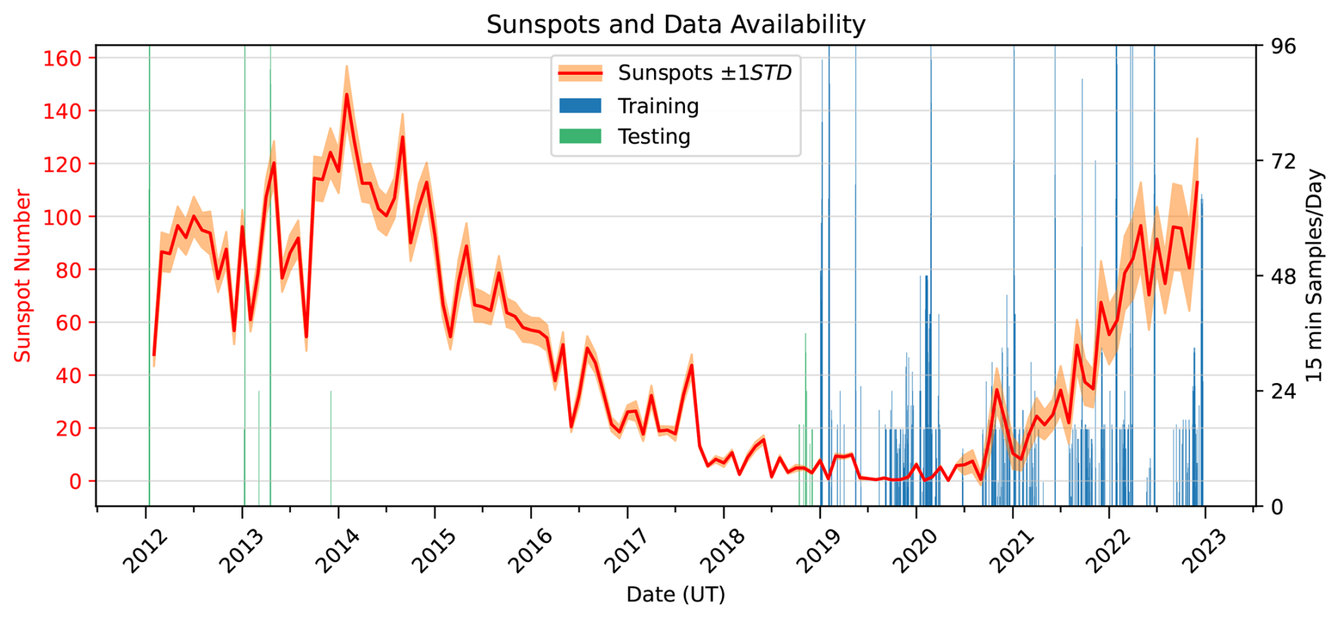
Figure 1 The distribution of 15 min intervals with EISCAT UHF data suitable for this study are shown along with the Sunspot number (incinerating solar phase). Blue lines mark days that are used for training the model while green lines displays testing days.

The EISCAT UHF profiles served as the “ground truth” for supervised training of our deep neural network (DNN). For each day with available EISCAT UHF measurements, we extracted the corresponding ionograms and geophysical parameters. Figure 1 shows the resulting data availability: between 2019 and 2022, 363 of 1452 d (25 %) yielded suitable data, providing 9040 of 139 392 possible hourly profiles (6.5 %), since many days contained data from experiments with partial daily coverage. The 2019–2022 data was selected due to the availability of simultaneous Digisonde and EISCAT data. Note that coverage is biased away from summer months due to reduced EISCAT usage during summer. This results in a dataset that is not balanced across all seasons. Furthermore, the training dataset is dominated by solar minimum and rising-phase conditions. To partially address this issue, we reserved data from the previous solar maximum and data from 2018 as an independent test set, containing 1177 samples. This enables evaluation of the model under contrasting solar cycle conditions. In future work, we aim to curate a more balanced dataset across both seasonal and solar-cycle variations to further improve model generalization. Our neural-network outputs were evaluated against ionogram-derived electron-density estimates from ARTIST 4.5 (Reinisch et al., 2005) and E-CHAIM's n_e(z) model predictions (Themens et al., 2017).

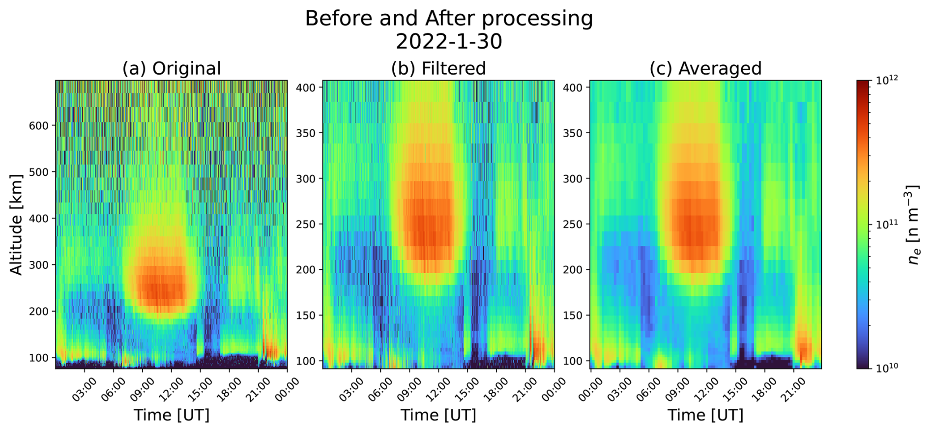
Figure 2 Example electron density profiles measured by the EISCAT UHF on 30 January 2022, illustrating the data processing steps. The left panel (a) shows the original extracted profiles, including unclipped measurements with noise and outliers. The middle panel (b) shows the profiles after outlier detection using PCA and IQR methods, followed by filtering of the detected outliers with a 2D median filter (in altitude and time) with kernel = (5 × 5). The right panel (c) shows the final profiles after averaging over 15 min intervals to match the temporal resolution of the Tromsø Digisonde.

2.1 The EISCAT Tromsø Ultra High-Frequency Radar

The EISCAT facility at Ramfjordmoen in Tromsø is one of the few high-latitude ISR stations located in the auroral zone (69.6° N, 19.2° E). The UHF radar consists of a 32 m antenna and operates in the 930 MHz band with a peak power of 2.0 MW. It measures ionospheric plasma parameters through several standard experiments (Lehtinen and Huuskonen, 1996). In this study, only data from runs of the standard experiment “beata” have been used. This experiment provides data with a minimum time resolution of 5.0 s over a range span of 49–693 km (Tjulin, 2017). One-minute-averaged plasma parameters for all available beata experiments, outlined in Fig. 2, were extracted from the public Madrigal database (Madrigal Database, 2025) for further processing. Only the measurement time (t), radar range (r), electron density (n_e), and measurement error (σ) were processed. We discarded electron-density profiles measured at zenith angles exceeding 20° to focus on near-vertical scattering, thereby excluding most scanning experiments. Figure 2 (first column) illustrates the extracted profiles for a day with full 24 h coverage.

The processed profiles were clipped to altitudes between 90 and 400 km to exclude D-region and upper F2-region activity, as measurements above 400 km contain little useful information for this study. The profiles were then re-interpolated onto the most common altitude grid in the dataset, consisting of 27 points. To remove NaN and ±∞ values (from failed ISR spectrum fits), we applied a simple in-painting procedure to interpolate or extrapolate these values. Additionally, a custom outlier-filtering script (see Appendix A) was used to detect and correct any remaining outliers in the n_e profiles, which may arise from noise or calibration issues.

Because the TGO ionosonde produces ionograms at least every 15 min, we averaged the EISCAT UHF profiles over 15 min intervals to match the ionosonde's time resolution (see third column in Fig. 2). Some intervals contained intermittent gaps; in those cases, we averaged all available measurements. Although the UHF data are averaged over a 15 min interval, each ionogram sweep requires 7–8 min, with much shorter dwell times at individual frequencies. Thus, under highly dynamic conditions the ionosphere may significantly change between the lowest and highest frequencies within a single sweep, making direct comparison with EISCAT UHF measurements complicated.

2.2 The Tromsø Geophysical Observatory Ionosonde

Ionospheric soundings have been performed in Tromsø for nearly a century. Hosted by the Auroral Observatory, Sir Edward Appleton established himself with an ionosonde during the Second International Polar Year (1932–33). Blueprints of this instrument were given to the observatory, a new instrument was built, and permanent soundings began in 1935. Over the years, five different ionosondes have been operated in Tromsø, producing one of the longest continuous time series in the world (Hall and Hansen, 2003). In 1992, a Lowell Digisonde DPS system (Reinisch et al., 1992) was acquired, featuring autoscaling capability via the ARTIST software (Reinisch et al., 2005; Galkin et al., 2008). The 1992 system underwent several software and hardware upgrades in 1998, 1999, 2001, and 2005. From 2005 to 2022, ARTIST 4.5 (Reinisch et al., 2005) served as the automatic ionogram scaler. In December 2022, the system was upgraded to a Digisonde DPS-4D (Reinisch et al., 2008) and has since been running ARTIST 5.0 (Galkin and Reinisch, 2008). For this work, however, we use data from the previous system (2005–2022), scaled with ARTIST 4.5. This allows us to take advantage of the large EISCAT dataset available from this period, providing the needed data volume to develop a reliable model.

The TGO digisonde (69.6° N, 19.2° E) is located approximately 525 m from the EISCAT UHF radar. The system operates in the upper medium-frequency (MF) to high-frequency (HF) bands with a range resolution of 5 km and a peak power of 300 W. The transmitter is connected to a crossed-rhombic antenna suspended by a ∼ 50 m tower, and reception is performed using four crossed-loop antennas. The digisonde transmits HF pulses into the ionosphere to determine the frequencies, f_s, at which wave reflections occur. It sweeps from 1 to 16 MHz, averaging 16 pulses for each frequency, taking up to 7 min with a 50 kHz step size. Using standard interferometric techniques, the angle of arrival of the backscattered signal is used to separate vertical from oblique backscatter. Electron densities are then obtained from the O-mode reflection at each virtual height through the relationship: $f_s\approx \mathrm{8.98}\sqrt{n_{\mathrm{e}}}$, where the plasma density n_e is in m⁻³ (Breit and Tuve, 1926; Davies, 1965).

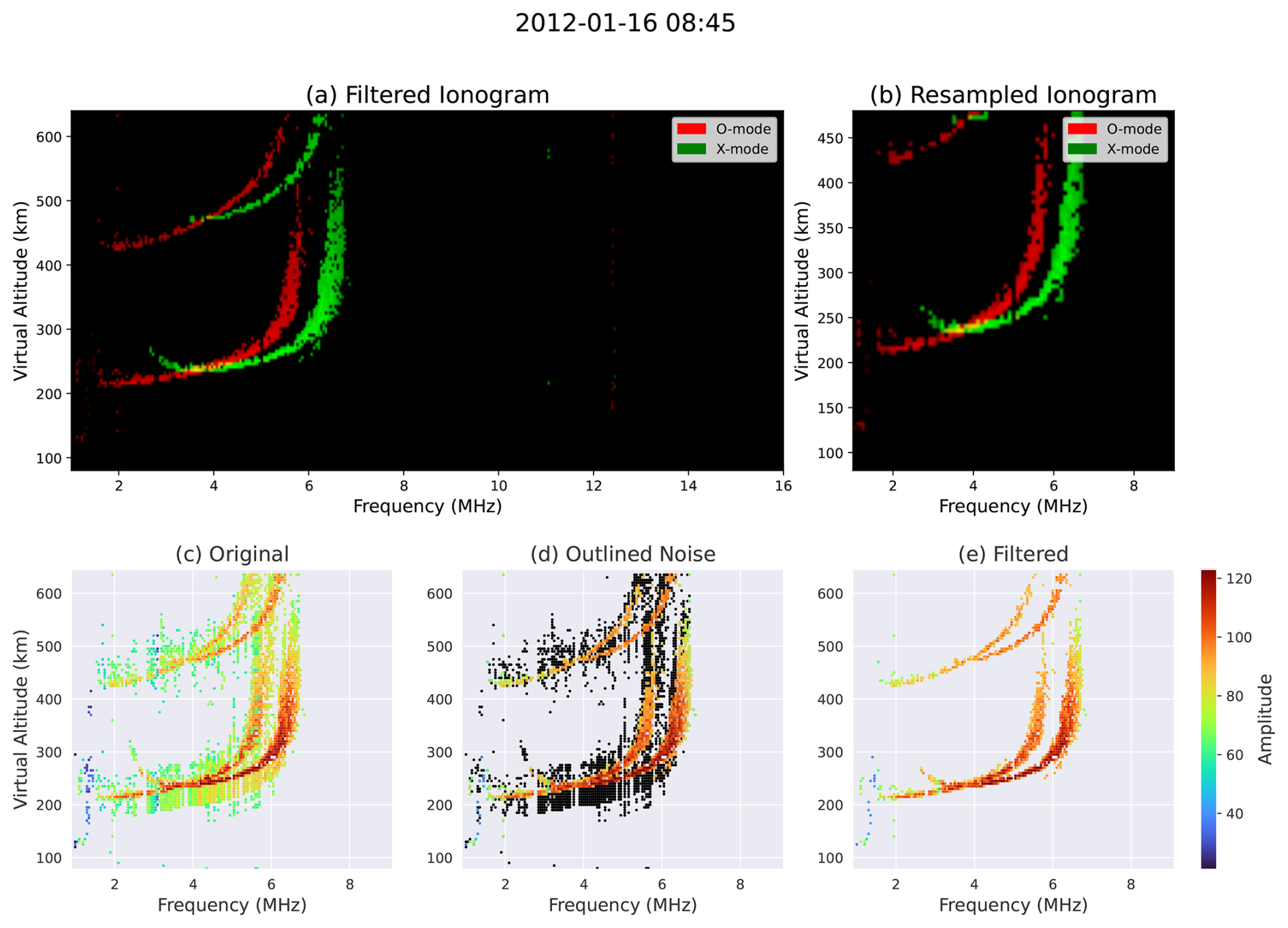
Figure 3 Top row: The left panel (a) shows the original ionogram from the TGO ionosonde, with O-mode echoes in red and X-mode echoes in green, plotted as a function of frequency (x-axis) and virtual altitude (y-axis). The right panel (b) shows the resampled ionogram, remapped onto an 81 × 81 grid with altitudes clipped to 80–480 km and frequencies limited to below 9 MHz. Bottom row: The filtering process in three stages. The left panel (c) presents the original ionogram with noise around the echoes. The middle panel (d) highlights the detected noise in black. The right panel (e) shows the cleaned ionogram, with echo strength indicated by color intensity.

SAO-Explorer, the standard Digisonde analysis tool, was used to extract ionogram data for further processing. We extracted frequencies, virtual ranges, amplitudes, polarizations, and zenith angles to construct ionogram images. Vertical echoes with polarization ± 90° were classified as O- and X-mode reflections, respectively. Using the extracted frequencies and virtual ranges, standard RGB images of size 113 × 301 × 3 were constructed, assigning O-mode to the red channel, X-mode to the green channel, and leaving the blue channel empty. Virtual ranges were clipped between 80 and 480 km to approximately match the altitude range of the ISR n_e profiles described in Sect. 2.1. The upper altitude limit was set to 480 km as ionosondes measure virtual heights and not actual heights, thus, allowing for the increasing difference between virtual and actual heights when nearing the F region maximum. Frequencies above 9 MHz were discarded, as few ionograms during this phase of the solar cycle contain f_OF2 above that threshold. Finally, a resampling grid was applied to produce symmetric ionogram images of shape 81 × 81 × 3. Figure 3 illustrates an example before and after processing.

Furthermore, during processing we found that ionograms measured before 2015 contained substantial noise around the X- and O-mode echoes (see Fig. 3c). These noisy echoes, reminiscent of leakage or a disconnected Rx antenna, could degrade model performance because it does not reflect the distribution of electron-density profiles in the training data. We therefore filtered these ionograms by discarding all pixels whose amplitude A_f,i at frequency f and image height i is less than 75 % of the maximum amplitude at that frequency. In other words, we retained only pixels satisfying the condition: $A_{f,i}\ge \mathrm{0.75}{max}_i\left(A_{f,i}\right)$.

2.3 Geophysical Parameters

A curated dataset of geophysical parameters was collected to characterize solar and geomagnetic activity. These parameters serve as inputs to the machine-learning network alongside ionogram data, facilitating the development of a baseline ionospheric model that is adjusted when an accompanying ionogram is available. This approach enables estimation of ionospheric plasma densities even during intervals without ionogram observations, thereby enhancing the network's robustness and supporting continuous, long-term operation.

Table 1 Solar and geophysical parameters used in the model.

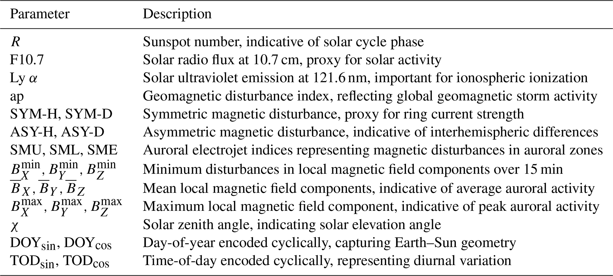
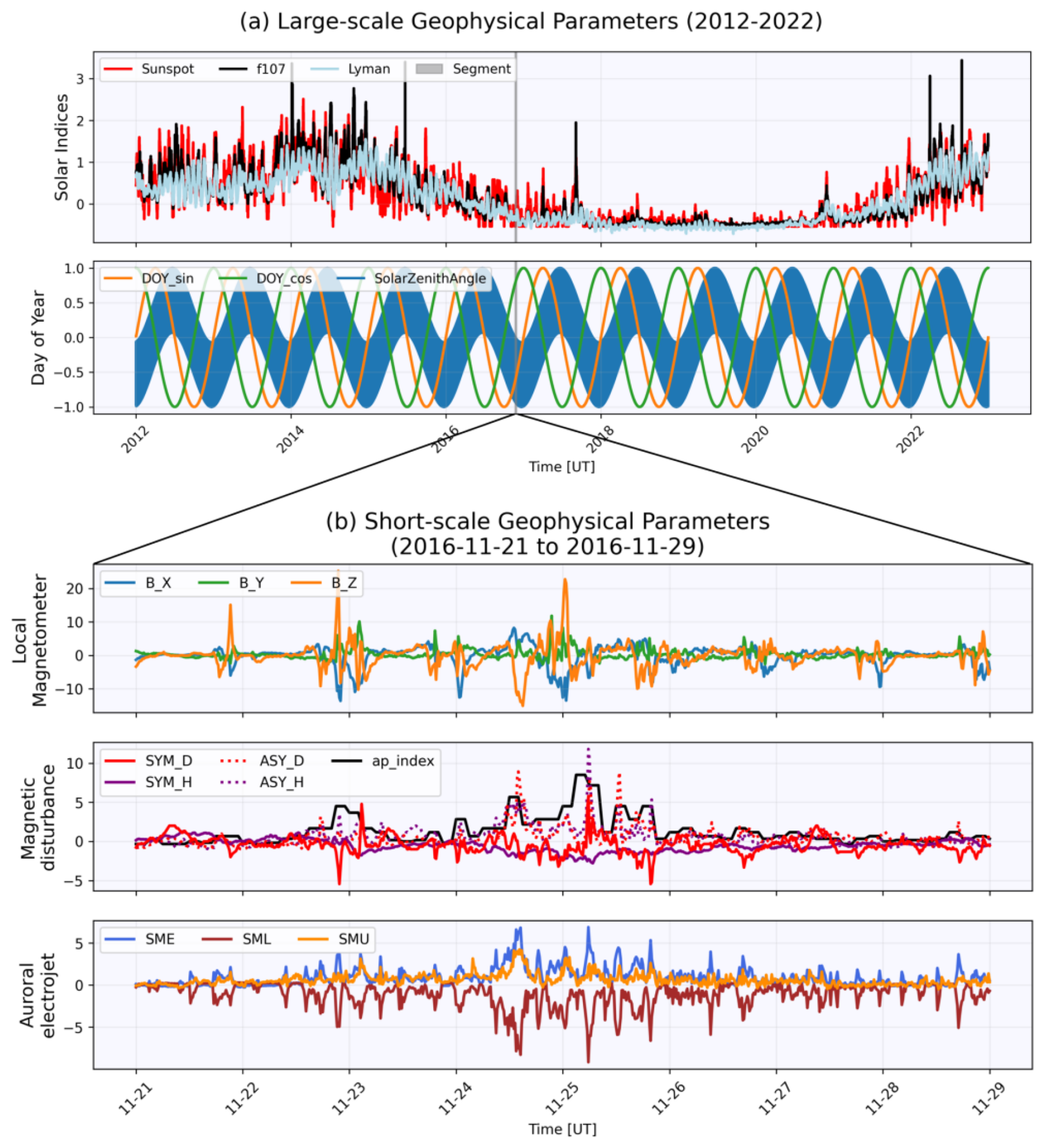
Figure 4 Time series of geophysical parameters. (a) Normalized large-scale solar parameters: sunspot number (red), F10.7 (black), and Lyman-α irradiance (light blue), along with the day-of-year (DOY) and solar zenith angle at Tromsø, plotted from 1 January 2012 to 31 December 2022. (b) A shorter interval showing additional normalized parameters: local magnetic-field components, ring-current indices, the Ap index, and auroral electrojet indices.

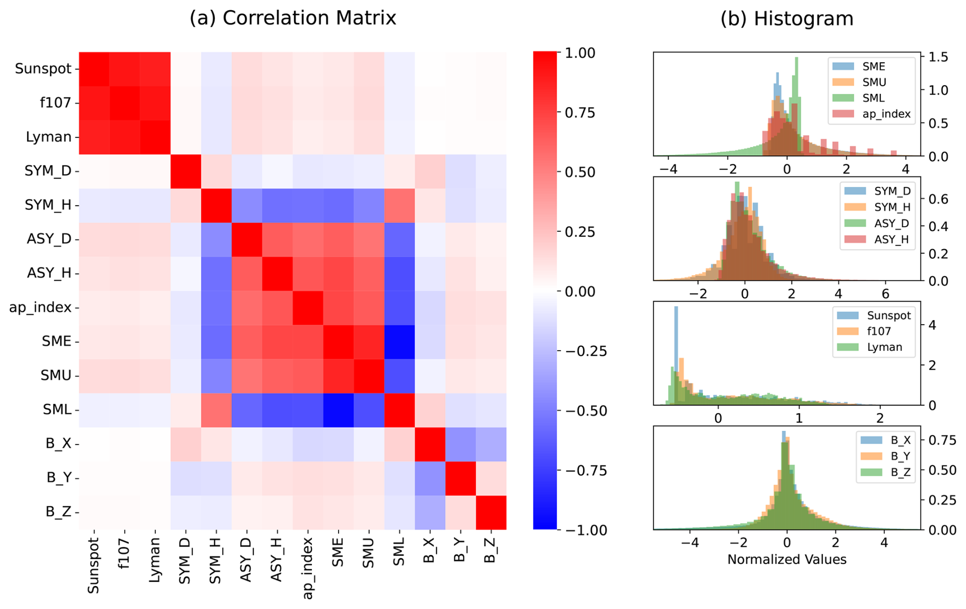
Figure 5 Overview of correlation and distribution of geophysical features from 2012 to 2022. (a) Correlation matrix of geophysical parameters excluding the time features and the min/max B-field features. (b) Histograms exhibiting the distribution for each feature category. i.e, Auroral electrojet, Magnetic disturbance, solar activity and B-field.

In total, 25 parameters were selected to capture solar, global, auroral and local geophysical conditions. Solar activity indices (R, F10.7, and Ly-α), ring-current indices (SYM-D, SYM-H, ASY-D, and ASY-H), and the ap index were obtained from the OMNIWeb database (National Aeronautics and Space Administration, 2025), while auroral electrojet indices (SMU, SML, and SME) were retrieved from SuperMAG (SuperMAG Database, 2025). Local magnetic-field parameters were calculated from magnetometer observations in Tromsø, Norway, provided by TGO (TGO Database, 2025). The magnetometer is located approximately 14 km northwest of the co-located EISCAT ISR and TGO ionosonde. The full list of parameters is summarized in Table 1 and plotted in Fig. 4. The correlation matrix (Fig. 5) reveals that some indices are nearly perfectly correlated, for example, sunspot number, F10.7, and Ly-α irradiance have correlation coefficients above 0.9. Still, all parameters are retained, as the computational cost of including each is negligible.

The cyclic parameters, day-of-year, time-of-day, and solar zenith angle, were normalized to the range $[-\mathrm{1},\mathrm{1}]$. All other geophysical parameters were normalized using robust scaling. For each parameter p_i, the scaled value ${\stackrel{\mathrm{̃}}{p}}_i$ is given by

$$\begin{array}{}\text{(1)}& {\stackrel{\mathrm{̃}}{p}}_i={\displaystyle \frac{p_i-\text{median}\left(p_i\right)}{\text{IQR}\left(p_i\right)}},\end{array}$$

where IQR(p_i) and median(p_i) are the interquartile range and median of p_i, computed over the dataset spanning one solar cycle (2012–2022).

3 Deep Learning Methodology

This section presents the multi-modal neural network designed to estimate the electron-density profiles, n_e(z), from ionograms and geophysical parameters. We describe the machine-learning and pattern-recognition techniques employed and detail the network architecture, which processes both scalar geophysical inputs and ionogram images.

3.1 Multi-Modal Neural Networks

The goal of this study is to estimate ionospheric electron-density profiles from corresponding ionogram images and geophysical parameters. We formulate this as a regression problem: find a function f that takes an ionogram I and parameter vector p as inputs and produces the profile n_e(z) as output. In practice, we model

$$\begin{array}{}\text{(2)}& n_{\mathrm{e}}\left(z\right)={\mathrm{10}}^{f(I,\mathit{p})}\end{array}$$

This defines a mapping between our input domains and the output domain:

$$\begin{array}{}\text{(3)}& f:(\mathbb{I},\mathbb{P})\to {\mathbb{N}}_{\mathrm{e}},\end{array}$$

where 𝕀 is the ionograms of size $H\times W\times C$ (here 81 pixel × 81 pixel × 2 pixel), ℙ is the d=25 geophysical feature vector (see Sect. 2), and ℕ_e is the electron-density profiles at the 27 considered height steps.

However, deriving the function f is challenging both because the inverse problem is highly non-linear and because of the complex behaviour of the high-latitude ionosphere, especially during periods of auroral activity. Consequently, exploring machine learning, in particular neural networks (NNs), is appropriate for developing a mapping that captures these non-linear, complex relationships. A key property of NNs is their ability to approximate any non-linear function given sufficient hidden layers, neurons, and well-chosen hyperparameters (Goodfellow et al., 2016, Chapter 6). In this work, we take advantage of this property to develop a multi-modal neural network (MMNN) that combines subnetworks trained to extract relevant features from both ionograms and geophysical parameters. Thus, our regression is defined as:

$$\begin{array}{}\text{(4)}& {\widehat{n}}_{\mathrm{e}}\left(z\right)={\mathrm{10}}^{f\left(\right[h(I;\mathit{\varphi }),g(p;\mathit{\phi })];\mathit{\theta })},\end{array}$$

where h (with parameters ϕ) processes the ionogram, g (with parameters φ) processes the geophysical vector, and f (with parameters θ) combines their embeddings to predict n_e(z).

This multi-modal configuration enables the MMNN to learn a richer latent representation by integrating different data sources, improving prediction accuracy (Huang et al., 2021). Moreover, the network can adapt to degraded or missing data in one modality by relying more heavily on the other. For example, if an ionogram is noisy or incomplete, the MMNN will predominantly base its density estimate on the geophysical inputs.

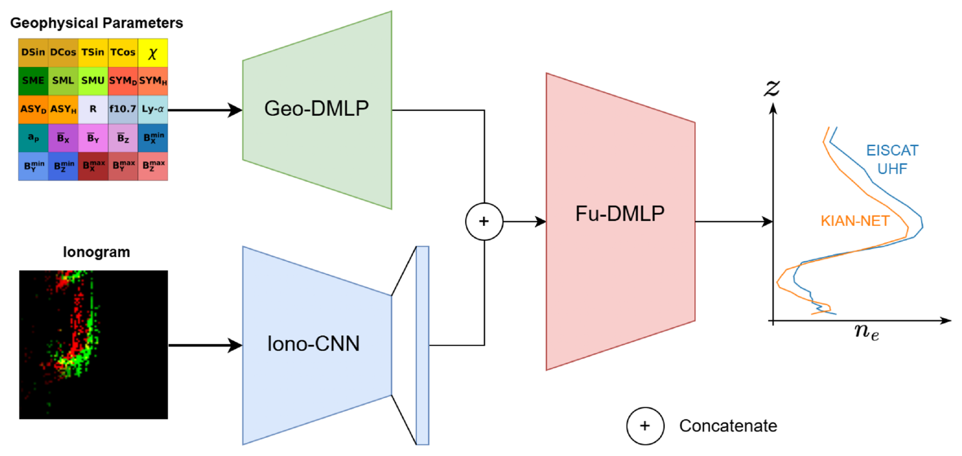
Figure 6 KIAN-Net architecture: A multi-modal neural network combining Iono-CNN for ionogram feature extraction, Geo-DMLP for geophysical parameter processing, and Fu-DMLP for feature fusion and final electron-density prediction.

3.2 Network Architecture

Our MMNN consists of three networks: (1) a Convolutional Neural Network (CNN) (Goodfellow et al., 2016, Chapter 9) to extract spatial features from ionogram echoes, (2) a Deep Multi-Layer Perceptron (DMLP) to extract scalar features from the geophysical parameters, and (3) a fusion DMLP that learns from the concatenated features of the previous two networks. We refer to these networks as Iono-CNN, Geo-DMLP, and Fu-DMLP, respectively, to simplify notation. Together, they constitute KIAN-Net (Kian's Ionospheric Assimilative Neural Network). Figure 6 provides an overview of the KIAN-Net architecture.

Figure 7 The Iono-CNN architecture: a 4-block convolutional neural network designed to extract spatial features from 3-channel (RGB) ionograms using stacked layers of Conv2D, BatchNorm2D, ReLU activation, and MaxPool2D. The diagram was made using the software developed by Iqbal (2018).

3.2.1 Iono-CNN

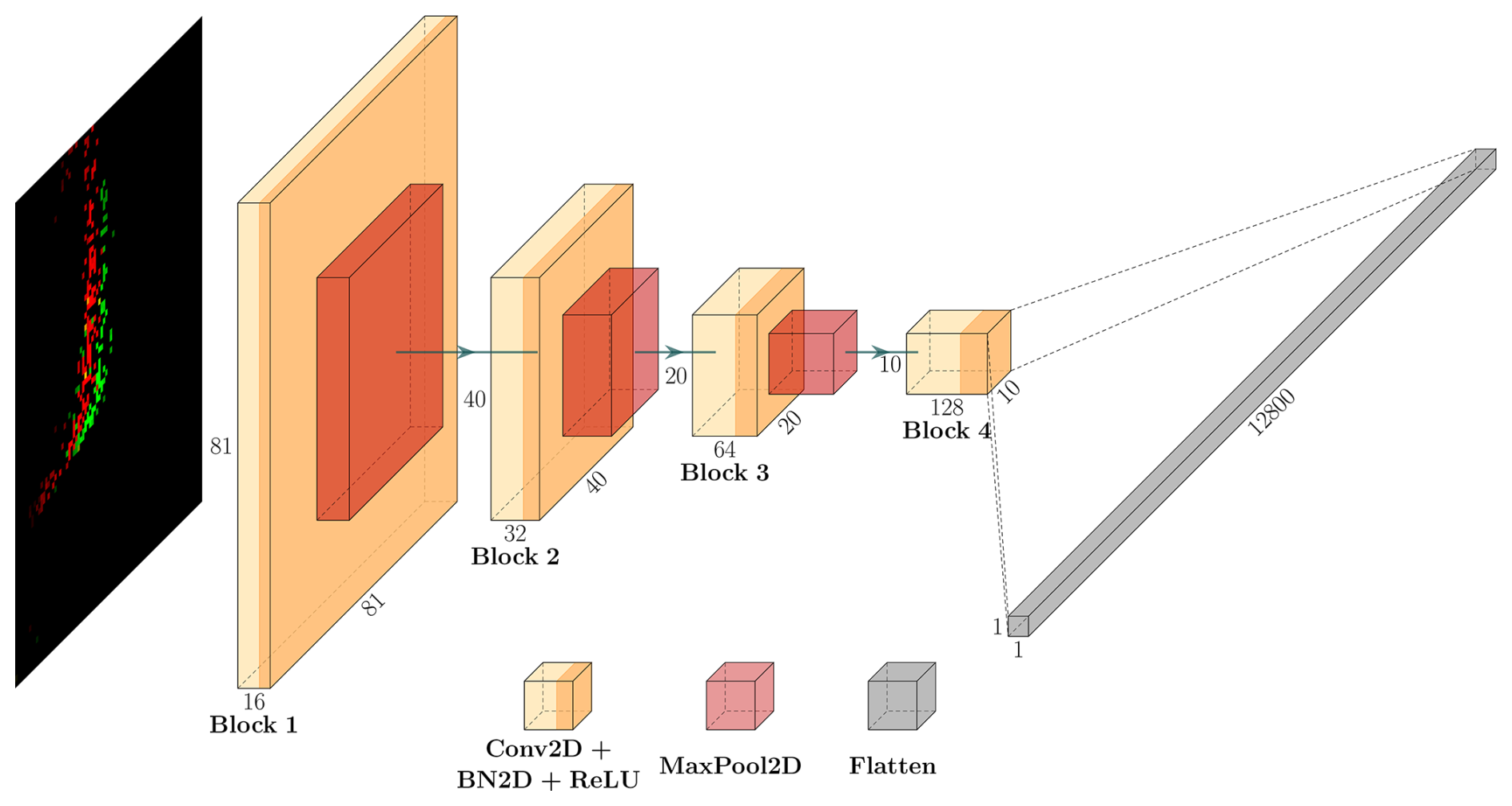
CNNs are able to extract features from ionograms containing E- and F-region echoes, as shown by Kvammen et al. (2024). Although they used single-channel ionograms, their work inspired us to build a CNN for three-channel (RGB) ionograms. Our Iono-CNN (Fig. 7) comprises four blocks, each containing:

• a Conv2D layer with 3 × 3 filters, stride 1, and padding 1;

• a BatchNorm2D layer;

• a ReLU activation (Nair and Hinton, 2010), which introduces nonlinearity while limiting outputs to [0,∞);

• a MaxPool2D layer with a 2 × 2 window (except in the final block).

We initialize all weights with He (Kaiming) initialization (He et al., 2015) to preserve variance through the ReLU nonlinearity. In the final layer, the feature maps are flattened into a 12 800-dimensional vector. The BatchNorm2D layers both accelerate convergence and smooth the loss surface by reducing internal covariate shift (Ioffe and Szegedy, 2015). Finally, the MaxPool2D layers downsample feature maps by selecting the maximum in each 2 × 2 window, the max-pooling lowers computational cost and captures spatially invariant dominant features (Goodfellow et al., 2016, Chapter 6).

3.2.2 Geo-DMLP

The Geo-DMLP maps 25 geophysical state parameters (Sect. 2.3) into a higher-dimensional (1024-dimensional) feature vector for estimating electron density, n_e(z). The network comprises five fully connected (FC) layers, each of which applies:

• a fully connected layer with trainable weights and biases

• batch normalization to reduce internal covariate shift (Ioffe and Szegedy, 2015)

• a ReLU activation (Goodfellow et al., 2016, Chapter 6) to introduce nonlinearity

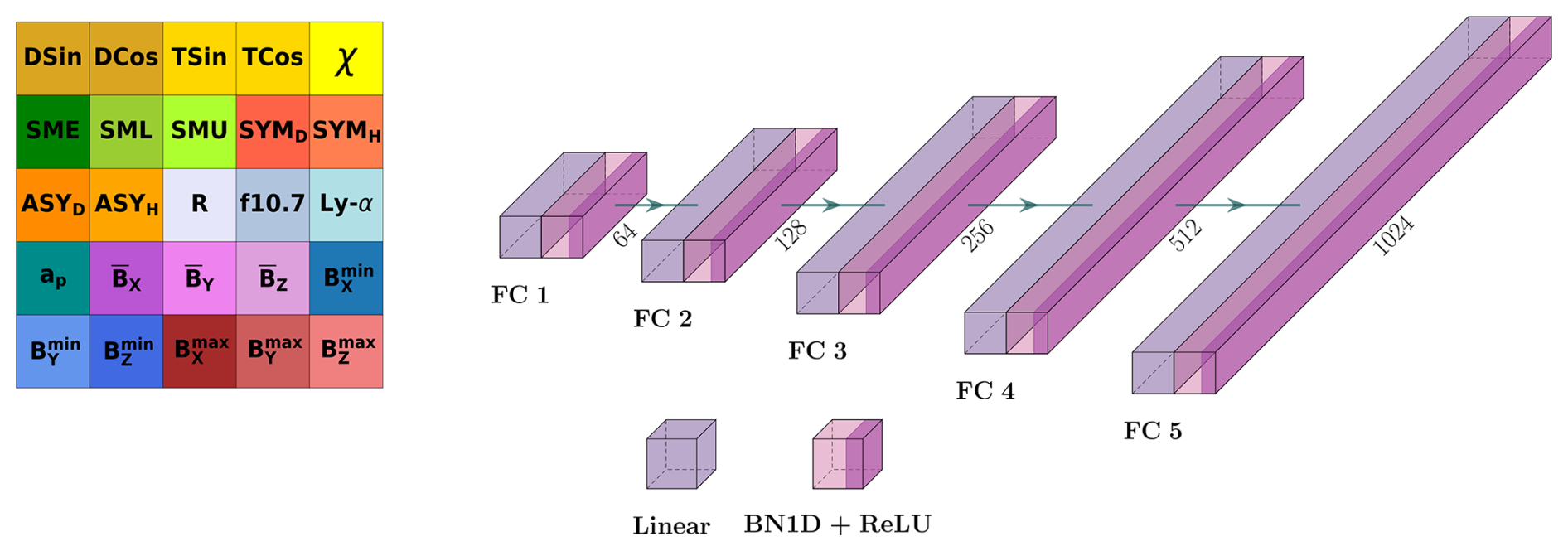
Figure 8 Geo-DMLP architecture: five fully connected layers transforming 25 geophysical inputs into a 1024-dimensional feature vector using FC layers, batch normalization, and ReLU activations. Inputs are color-coded by relevance (e.g., magnetic field components in shades of purple). The diagram was made using the software by Iqbal (2018).

The complete architecture is shown in Fig. 8.

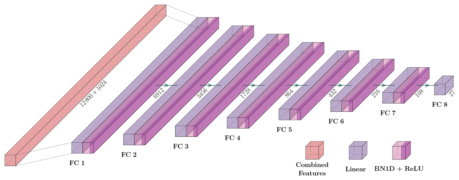
Figure 9 Fu-DMLP architecture: an 8-layer, encoder-style FC network that fuses the 12 800 and 1024-dimensional feature vectors from Iono-CNN and Geo-DMLP to predict 27 electron-density values over the 90–400 km range. The model uses FC layers, BatchNorm1D, and ReLU activations for stable training and progressive dimensionality reduction. Diagram by Iqbal (2018).

3.2.3 Fu-DMLP

To fuse the features from Iono-CNN and Geo-DMLP, we introduce Fu-DMLP (Fig. 9). The network takes the concatenated feature vector (12 800 + 1024 dimensions) and predicts 27 electron-density values across the 90–400 km range without explicit altitude inputs. Fu-DMLP is an eight-layer fully connected network arranged in an encoder-like fashion. In this model, each successive layer has approximately half the neurons of its predecessor, forming a bottleneck that compresses the representation before the final 27-dimensional output. Each layer consists of:

• a fully connected layer with trainable weights and biases;

• BatchNorm1D for stable activations (Ioffe and Szegedy, 2015);

• a ReLU activation (Goodfellow et al., 2016, Chapter 6) to introduce nonlinearity.

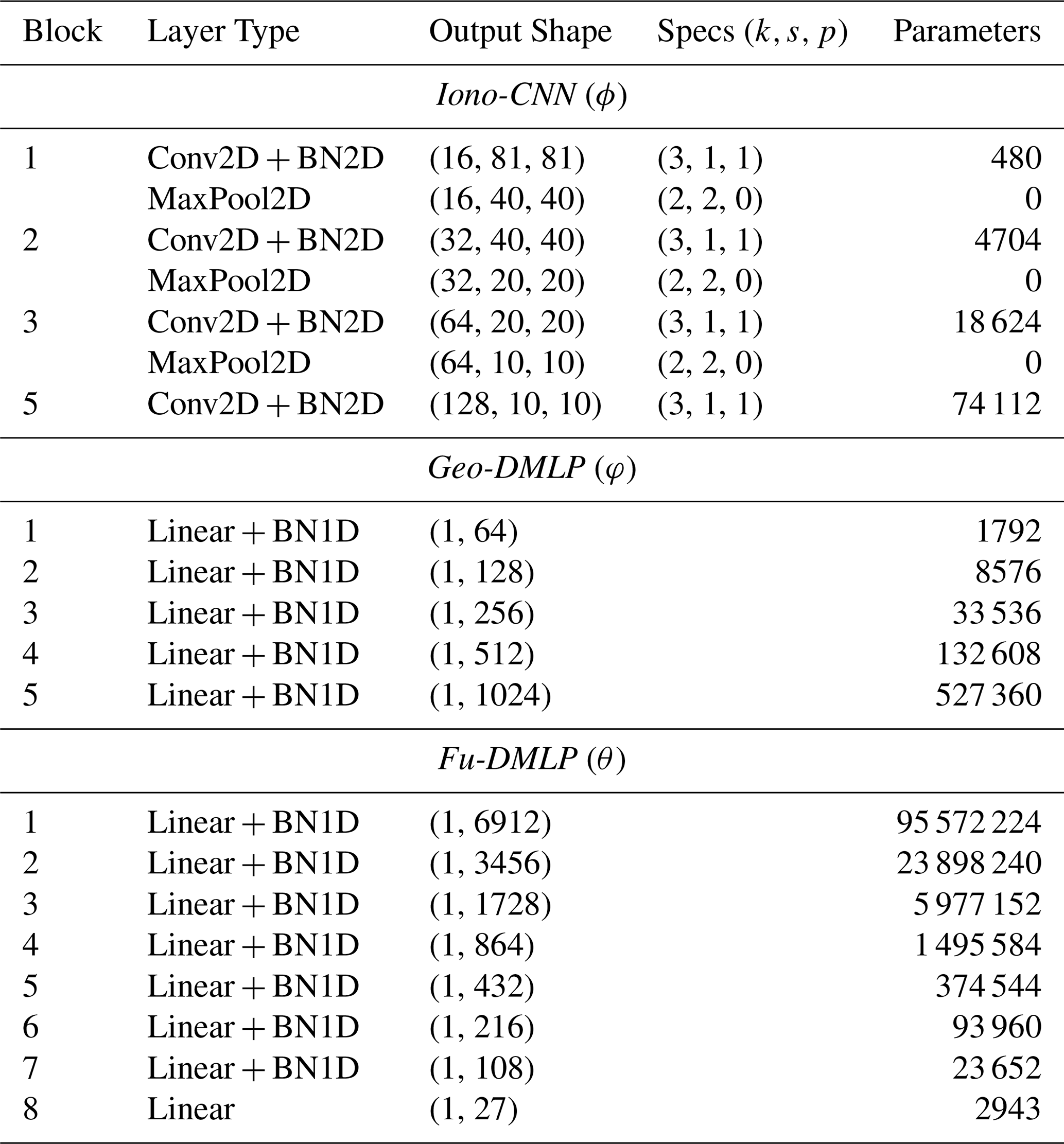
Table 2 Architectural specifications of KIAN-Net's three-component MMNN. Iono-CNN processes 3-channel RGB ionograms through four convolutional blocks (Conv2D + BatchNorm + ReLU + MaxPool) with 3 × 3 kernels. Geo-DMLP trains geophysical parameters through five linear layers, also including batch normalization in 1D (BN1D). Fu-DMLP combines features from both networks and is trained to predict 27 electron density values. Parameter counts include BatchNorm weights within preceding layers. Total learnable parameters: 127 438 299.

3.3 Training

The predictions generated by KIAN-Net were evaluated against the ground truth using the Huber loss function (Huber, 1964). This loss function combines the properties of both Mean Squared Error (MSE) and Mean Absolute Error (MAE), where small residuals are treated quadratically, while large residuals are treated linearly. This makes the network more robust to outliers (Terven et al., 2023), which can lead to more stable training that effectively damps the impact of short-scale ionospheric activities. This approach further reduces the impact of noisy observations and faulty data on the network gradients. The electron density profiles were normalized with log₁₀ in order to scale down in magnitude. Redefining the expression from Hastie et al. (2009), Huber Loss is expressed as:

$$\begin{array}{}\text{(5)}& L_{\mathit{\delta }}\left(a\right)=\left\{\begin{array}{ll}\frac{\mathrm{1}}{\mathrm{2}}(a{)}^{\mathrm{2}},& \text{if }\left|a\right|\le \mathit{\delta },\\ \mathit{\delta }\left|a\right|-\frac{\mathrm{1}}{\mathrm{2}}{\mathit{\delta }}^{\mathrm{2}},& \text{otherwise.}\end{array}\right.\end{array}$$

where a is the residual:

$$a={\log }_{\mathrm{10}}\left(n_{\mathrm{e}}\right(z\left)\right)-f\left(\left[h\right(I;\mathit{\varphi }),g(p;\mathit{\phi }\left)\right];\mathit{\theta }\right)$$

where n_e(z) are the true values, f are the model output values and δ>0 is a tunable hyperparameter that sets the transition point between MSE and MAE. We used the default value δ=1. In order to estimate the mapping function in Eq. (3), the optimal set of total KIAN-Net parameters $\widehat{\mathit{\omega }}$, where $[\widehat{\mathit{\theta }},\widehat{\mathit{\varphi }},\widehat{\mathit{\phi }}]\in \widehat{\mathit{\omega }}$, can be approximated by minimizing the total Huber Loss over N number of n_e profiles. This is mathematically defined as:

$$\begin{array}{}\text{(6)}& \begin{array}{rl}\widehat{\mathit{\omega }}=& {\text{arg\hspace{0.17em}min}}_{\mathit{\theta },\mathit{\varphi },\mathit{\phi }}\sum _{i=\mathrm{1}}^N\sum _{j=\mathrm{1}}^{\mathrm{27}}{L}_{\mathit{\delta }}\\ & \times \left({\log }_{\mathrm{10}}\right(n_{\mathrm{e}}\left(z_j\right))-f(\left[h\right(I;\mathit{\varphi }),g(p;\mathit{\phi }\left)\right];\mathit{\theta }\left)\right).\end{array}\end{array}$$

Optimization was performed using the Adaptive Moment Estimation (ADAM) algorithm (Kingma and Ba, 2014), which builds on the Stochastic Gradient Descent (SGD) algorithm, originally introduced by Robbins and Monro (1951). ADAM improves SGD by using adaptive learning rates, estimating first and second order momentum terms with exponentially decaying averages. These terms, mitigates the possibility of getting stuck in local minimas during training, as well as smoothening the corresponding loss surface. However, it is acknowledged that recent research propose convergence issues linked to ADAM for specific use cases (Reddi et al., 2019; Zou et al., 2021).

Both the network architecture and the training process were implemented using the PyTorch framework. The dataset was constructed by pairing ionograms and geophysical state parameters with the corresponding ground-truth electron-density profiles, forming sample triplets $\left(n_{\mathrm{e}}\right(z{)}_i,I_i,p_i)$. This dataset was then randomly split into training and validation sets with an $\mathrm{80}/\mathrm{20}$ ratio to mitigate splitting bias. Each set was loaded via PyTorch dataloaders: the training loader used a batch size of 256 and shuffled the samples after each epoch to reduce learning bias and improve generalization (Smith et al., 2020). For validation, the entire validation set was utilized as a single batch, with the sample order also randomized. The training ran over 350 epochs with an initial learning rate set to 0.01. For refined convergence, two schedulers were set at 200 and 300 epochs, reducing the learning rate to 0.001 and 0.0001, respectively.

4 Results

The global performance of KIAN-Net was evaluated by comparing its predictions n_e(z_i) with EISCAT UHF measurements from selected days in the years 2012, 2013, and 2018. The test dataset was entirely disjoint from the training dataset, using different years of data for training and testing. This approach ensures a fair evaluation of the model's ability to generalize to unseen geophysical conditions and solar cycle phases.

To determine how KIAN-Net's estimates of n_e(z_i) compare with existing methods, we included results from ARTIST 4.5 and E-CHAIM in our analysis. The E-CHAIM model was run with both the “storm” and “precip” flags enabled, meaning that global and auroral-zone information from the Ap, AE, and DST indices was used to estimate the electron density profile (Themens et al., 2017). We also generated estimates using each network component separately (Iono-CNN and Geo-DMLP) to assess their individual contributions and determine the relative influence of each input on the overall performance. To quantify goodness of fit, we used the testing dataset to compute the R² score, the root-mean-square error (RMSE), the Pearson correlation coefficient r_p, and the distance correlation r_d. A summary of these performance metrics are presented in Table 3.

Table 3 Comparison of five models using R²-score, RMSE, Pearson correlation (r_p), and distance correlation (r_d) metrics, averaged over all time steps in the testing dataset. KIAN-Net outperforms both its subcomponents (Iono-CNN and Geo-DMLP) and the baseline models (Artist 4.5 and E-CHAIM) across all metrics. Bold values indicate the best-performance.

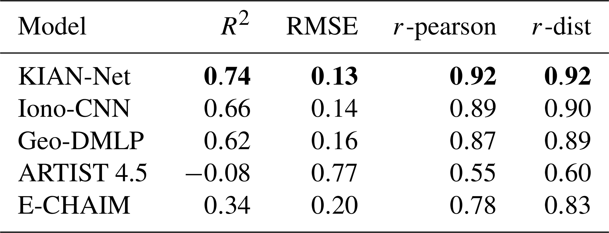
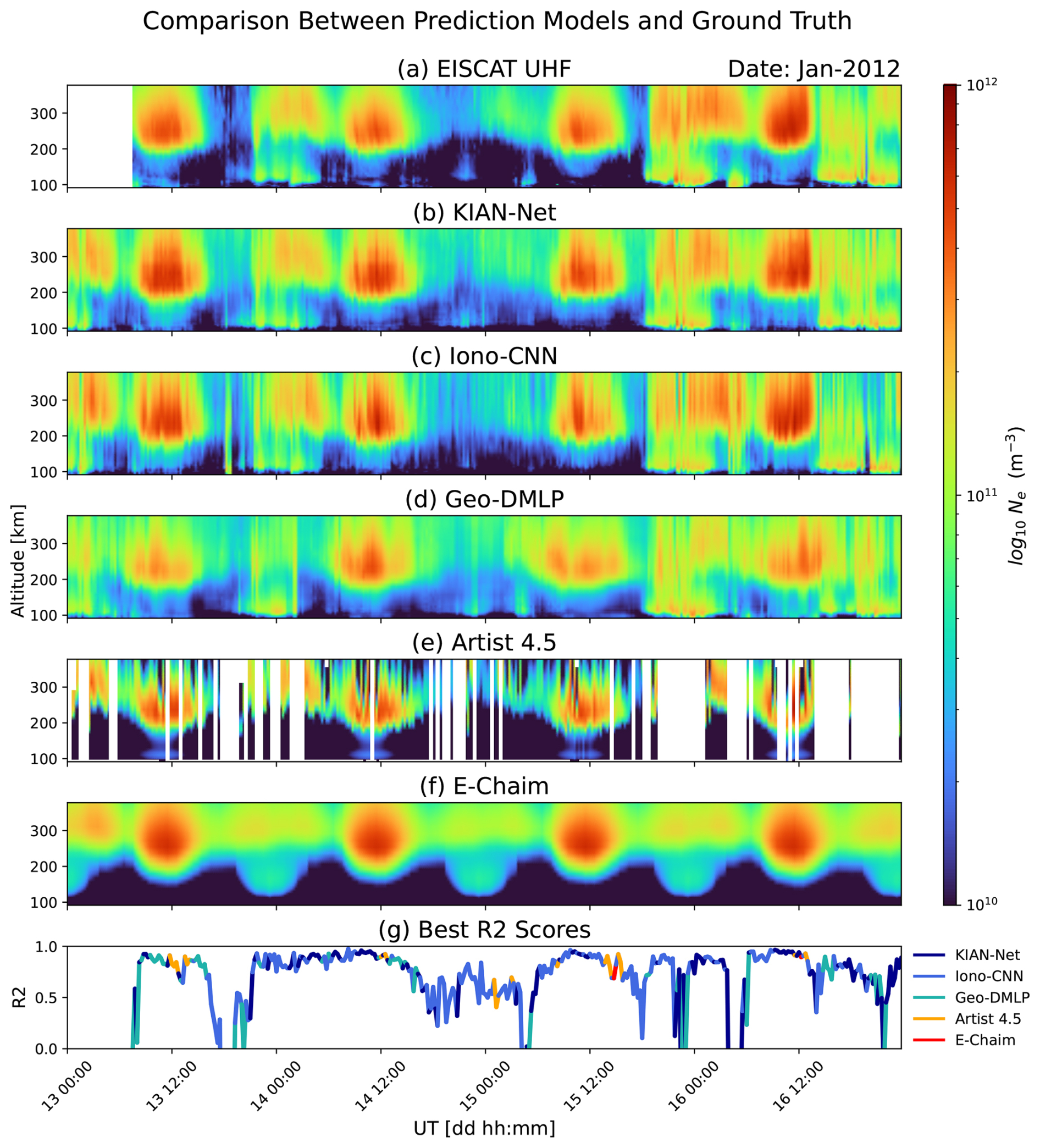
Figure 10 Comparison of electron-density profiles from 13 January 2012 to 17 January 2012 (00:00 UTC) against EISCAT UHF ground truth. (a) EISCAT UHF measurements of the electron density profiles. (b) Predictions made by KIAN-Net. (c) Predictions made by Iono-CNN. (d) Predictions made by Geo-DMLP. (e) Estimates made by ARTIST 4.5. (f) Estimates made by E-CHAIM. (g) The calculated R²-scores at each time step where the colours depict the model with the best corresponding R².

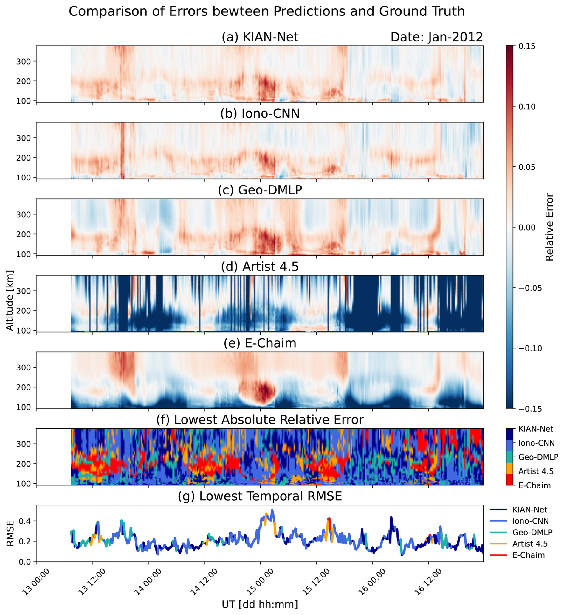
Figure 11 Relative error between model predictions and EISCAT UHF ground truth from 13 January 2012 to 17 January 2012 (00:00 UTC). (a) Relative error by KIAN-Net. (b) Relative error by Iono-CNN. (c) Relative error by Geo-DMLP. (d) Relative error by ARTIST. (e) Relative error by E-CHAIM. (f) Colour plot depicting the colour of the prediction with the least absolute relative error. (g) RMSE at each time step, with colors indicating the model achieving the lowest RMSE.

To illustrate model performances and further analyze the model outputs, we examine a four-day interval (13–17 January 2012) that captures full diurnal cycles and a representative range of geophysical activity. Results for this period are presented in Fig. 10, with corresponding relative errors in Fig. 11.

Visual inspection of Figs. 10 and 11 shows that all deep-learning models successfully approximate the electron-density profiles and agree well with the EISCAT UHF measurements. By direct comparison, KIAN-Net, Iono-CNN, and Geo-DMLP outperform ARTIST 4.5 and E-CHAIM on the test dataset, with superior quantitative metrics, as shown in Table 3. Overall, KIAN-Net, Iono-CNN, and Geo-DMLP achieve R² scores of 0.74, 0.66, and 0.62, respectively, while ARTIST 4.5 and E-CHAIM obtain R² of −0.08 and 0.34. Figure 10 also highlights that all models, including the deep learning models, struggle to estimate nighttime electron densities during weak auroral precipitation. There are several reasons for this. First, during low-density periods in the F region, such as under the ionospheric trough, ionograms often contain limited information about the electron density profile, particularly above auroral heights. The trough is typically associated with strong horizontal gradients and tilts in the ionosphere, which inhibit vertical-incidence signals from returning to the ionosonde receiver (Voiculescu et al., 2010; Zabotin et al., 2006). This limitation can be further enhanced by auroral absorption in the D-region, which reduces the signal-to-noise ratio of the ionosonde returns. Second, there is also a differences in sampling geometry, the EISCAT UHF radar provides altitude-resolved measurements within a narrow ∼ 1° field of view, whereas the Digisonde has a broader vertical field of view ∼ 30°. This difference, combined with the ionosonde's reduced sensitivity during trough and absorption conditions, makes direct comparisons between EISCAT profiles and ionogram-based estimates particularly challenging in the nighttime auroral region.

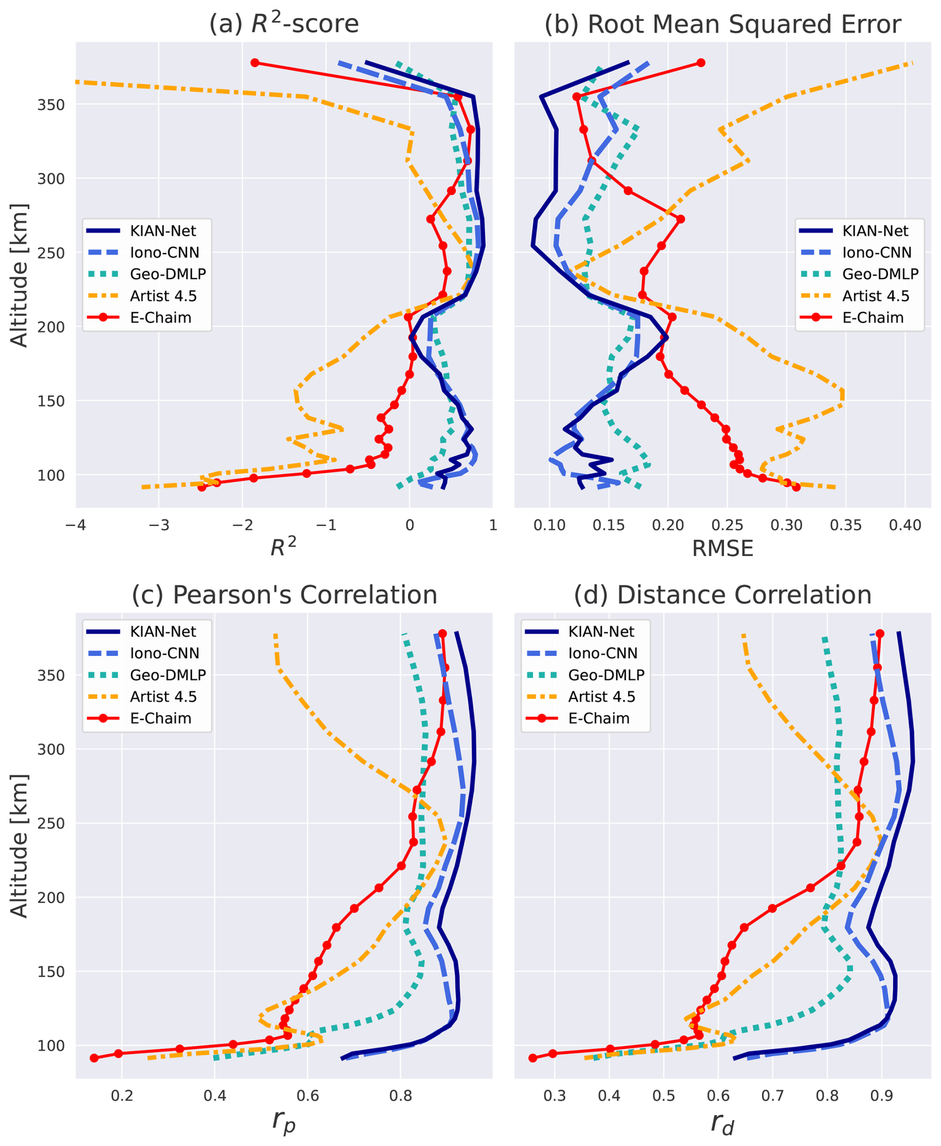
Figure 12 Calculated metrics between the models predictions (KIAN-Net, Iono-CNN, Geo-DMLP, ARTIST 4.5, E-CHAIM) and the EISCAT UHF electron density profiles along the temporal axis for each altitude ranging within 90–400 km. The performance metrics: (a) Calculated R²-score, (b) Root Mean Squared Error (RMSE), (c) Pearson's correlation coefficient (r_p), and (d) The Distance correlation (r_d), are shown as functions of altitude. Results are aggregated over all available time steps where EISCAT UHF has valid profiles (non-Nan values), with metrics calculated using normalized (0–1) electron density values. Higher R²/r_p/r_d and lower RMSE indicate better agreement with EISCAT UHF measurements.

Figure 12 presents the time-averaged performance metrics as a function of altitude. The metrics: R², RMSE, Pearson correlation (r_p), and distance correlation (r_d) are systematically better for the DL models at all altitudes below 350 km. In this region, ARTIST 4.5 often failed and was replaced by a constant n_e = 1 × 10⁸ m⁻³ to enable comparison with ISR observations. The performance gap is most pronounced in the E-region (100–160 km), where the KIAN-Net and Iono-CNN models achieve R²≳ 0.4 and RMSE≲ 0.2, whereas ARTIST 4.5 and E-CHAIM yield R²≪ 0 and RMSE≳ 0.2. This is further illustrated by the relative-error plots in Fig. 11d and e, which show that densities between 90 and 160 km are generally underestimated (blue shading). Correlation metrics also favour the DL models, with both r_p and r_d typically exceeding 0.90, and reaching ≥ 0.95 in the upper F-region for the KIAN-Net and Iono-CNN models, while ARTIST 4.5 and E-CHAIM exhibit correlations generally below 0.8.

5 Discussion

The estimates produced by KIAN-Net closely match those of Iono-CNN, indicating that the ionogram inputs dominate over the geophysical parameters used by Geo-DMLP. This is expected, since the ionogram traces contain direct information about the electron densities, whereas the relationship between electron densities and geophysical parameters is more indirect. Nevertheless, Geo-DMLP captures both the daily variation of the F-region and the auroral variation of the E-region n_e relatively well. At F-region heights, n_e is governed by the balance between recombination and photoionization, which to first order depends on EUV flux (captured by F10.7) and the solar zenith angle. For the test days, Geo-DMLP tends to overestimate the duration of the F-region, predicting higher n_e during both sunrise and sunset. We attribute this to significant day-to-day fluctuations of n_e due to variable ionospheric horizontal convection during these periods. Remarkably, Geo-DMLP also predicts E-region enhancements due to auroral precipitation, despite its limited information about the local ionosphere. The geophysical parameters most sensitive to auroral activity are the local magnetic-field fluctuations driven by the auroral electrojet. However, these fluctuations arise from currents spanning a much larger region than the localized E-region echoes detected by the ionogram. To further assess their role, we performed a preliminary absolute gradient impact analysis of the geophysical inputs. This analysis indicates that solar zenith angle and F10.7 contribute most strongly, followed by AE and local magnetic-field variations, consistent with their expected influence on F-region ionization and auroral precipitation. Although ionogram data dominate model performance, these results suggest that the geophysical parameters provide complementary and physically meaningful information. Further, our results show that the DL-models successfully captured nighttime electron density profiles with both E and F-region peaks, as further discussed in Appendix B.

ARTIST 4.5 systematically produced reasonable estimates of daytime bottom-side F-region densities. However, the quality of the topside densities is rather variable. This shortcoming stems from ARTIST's methodology, which derives an α-Chapman profile for the topside F-region peak using bottomside F-region densities. This approach is an oversimplification, especially during periods of high-energy deposition from the magnetosphere and loss of thermal equilibrium along the vertical column. During auroral activity, ARTIST 4.5 often fails to produce any n_e(z_i) estimates. When intense E-region ionization disrupts the ionosonde's ability to detect F-region echoes, ARTIST omits to make an electron density profile and instead scales the E-region as a sporadic E-layer.

In comparison, E-CHAIM, as an empirical mid- and high-latitude ionospheric model, generated continuous predictions throughout the test period. Using only the Ap, AE, and Dst indices as inputs, E-CHAIM does not respond to short-term or local variations, resulting in smoother n_e(z) profiles. Consequently, E-CHAIM does not fully capture day-to-day local variations of F-region densities and the rapidly varying auroral E-region densities. Near the foF2 peak, where all models perform reasonably well, KIAN-Net and Iono-CNN remain slightly superior, with R² scores typically above 0.95 and RMSE≈ 0.05. ARTIST 4.5 follows with R²≈ 0.75 and RMSE≈ 0.13, outperforming Geo-DMLP in this region. E-CHAIM shows weaker performance across most altitudes, except in the upper F-region (≥ 250 km), where its correlation coefficients reach ≳ 0.65.

There are several potential directions for future development of this method. First, incorporating additional EISCAT data from solar-maximum and summer conditions would balance the current dataset. Due to data availability, the considered dataset is weighted toward autumn, winter, and spring during the rising phase of the recent solar cycle. Dedicated summer campaigns should be conducted in the coming years to collect these missing observations. Second, extending this technique to include data from other ISR facilities, both across magnetic local time in the northern auroral zone (Sondre Strømfjord, Resolute Bay, Poker Flat, and EISCAT Svalbard) and at lower latitudes (Millstone Hill, Sanya, Arecibo, and Jicamarca), would broaden geographic and temporal coverage. For this task, it is not obvious if a single deep learning model should be trained with all available data to provide a global ionogram-inversion scheme, or if it is preferable with separate models for each IS-radar followed by an interpolation scheme, such as those used in Holt et al. (2002) and Zhang et al. (2005). Although KIAN-Net can operate using only ionograms or only geophysical parameters, we have not yet systematically evaluated how its performance degrades when one or more geophysical inputs are unavailable. Such “reduced-input” Geo-DMLP variants may effectively transition toward empirical models like E-CHAIM, this might make it possible to justify and make such models more responsive to geophysical conditions. Moreover, as computational resources increase, processing higher-resolution ionogram images with larger virtual-height ranges should further improve the quality of the estimates. Furthermore, E-CHAIM also includes an assimilative mode, A-CHAIM, which ingests ionosonde and GNSS-TEC data to adjust its output away from climatology, comparing A-CHAIM's assimilative performance with KIAN-Net would be of interest. In addition, incorporating further geophysical inputs into KIAN-Net, such as vertical TEC, the Polar Cap Index, and solar indices (e.g., F30 and MG II (Laštovička and Burešová, 2023)), may improve its accuracy. Finally, because ionograms may contain information about other plasma parameters, training KIAN-Net to predict electron and ion temperature profiles could extend its utility beyond density estimation.

6 Conclusions

We have presented a multi-modal neural-network, named KIAN-Net, to estimate ionospheric electron-density profiles from both ionogram images and geophysical parameters. The model was trained to learn the mapping from 25 readily available geophysical inputs and ionogram images to simultaneous electron-density profiles measured by the EISCAT UHF incoherent scatter radar in Tromsø. Its two subnetworks, Iono-CNN and Geo-DMLP, extract complementary features from the ionograms and geophysical state parameters, respectively. KIAN-Net and its two subnetworks performs favorably compared to the industry-standard ionogram-inversion algorithm (ARTIST 4.5) and the state-of-the-art high-latitude empirical ionospheric model (E-CHAIM). Notably, Geo-DMLP, which is trained only on geophysical parameters, effectively captures high-latitude spatial and temporal variability, caused by dynamic auroral precipitation and complex plasma convection, suggesting its utility as a local ionospheric model for Tromsø.

In total, over 10 000 ionogram–geophysical-parameter sample pairs were used to train and evaluate KIAN-Net. On an independent test set spanning multiple years, KIAN-Net achieved an R² of 0.74 against EISCAT observations, compared to R² = −0.08 for ARTIST 4.5 and R² = 0.34 for E-CHAIM. KIAN-Net also obtains RMSE≤ 0.17, Pearson correlation r_p≥0.92, and distance correlation r_d≥ 0.92. Detailed analysis shows that KIAN-Net provides robust and reliable electron density estimates (R² > 0.5) across diverse ionospheric conditions, including periods with significant auroral activity. Future work includes expanding the network to different latitudes and longitudes where ISR data are available and training it to predict additional plasma parameters (e.g., electron and ion temperatures) from the input data, further expanding the capabilities of the model.

Appendix A: Outlier-Filtering Procedure

The outlier-filtering procedure operates as follows. First, a principal component analysis (PCA) is applied to the collection of electron-density profiles for each individual day containing data. PCA is a dimensionality reduction technique that maps the original variables (electron densities at different altitudes) onto a new set of orthogonal axes, called principal components. These components are linear combinations of the original variables and are ordered so that the first component explains the largest variance in the dataset, the second the next largest, and so forth. By keeping only the first two components, each profile is represented in a compact two-dimensional form that captures its dominant variability, even though the components no longer correspond directly to the original physical variables (altitude and density). Second, outliers are detected using the interquartile range (IQR) method, where any value lying outside the lower and upper fences at Q1−1.5 IQR or Q3+1.5 IQR, with $\text{IQR}=\text{Q3}-\text{Q1}$, is flagged as a potential outlier. Finally, each identified outlier profile is processed by applying a 2D median filter (in altitude and time) with kernel = (5 × 5), which smooths the outlier by matching neighboring values while preserving the overall profile shape. Figure A1 shows an example of this filtering on EISCAT UHF profiles from 31 March 2022.

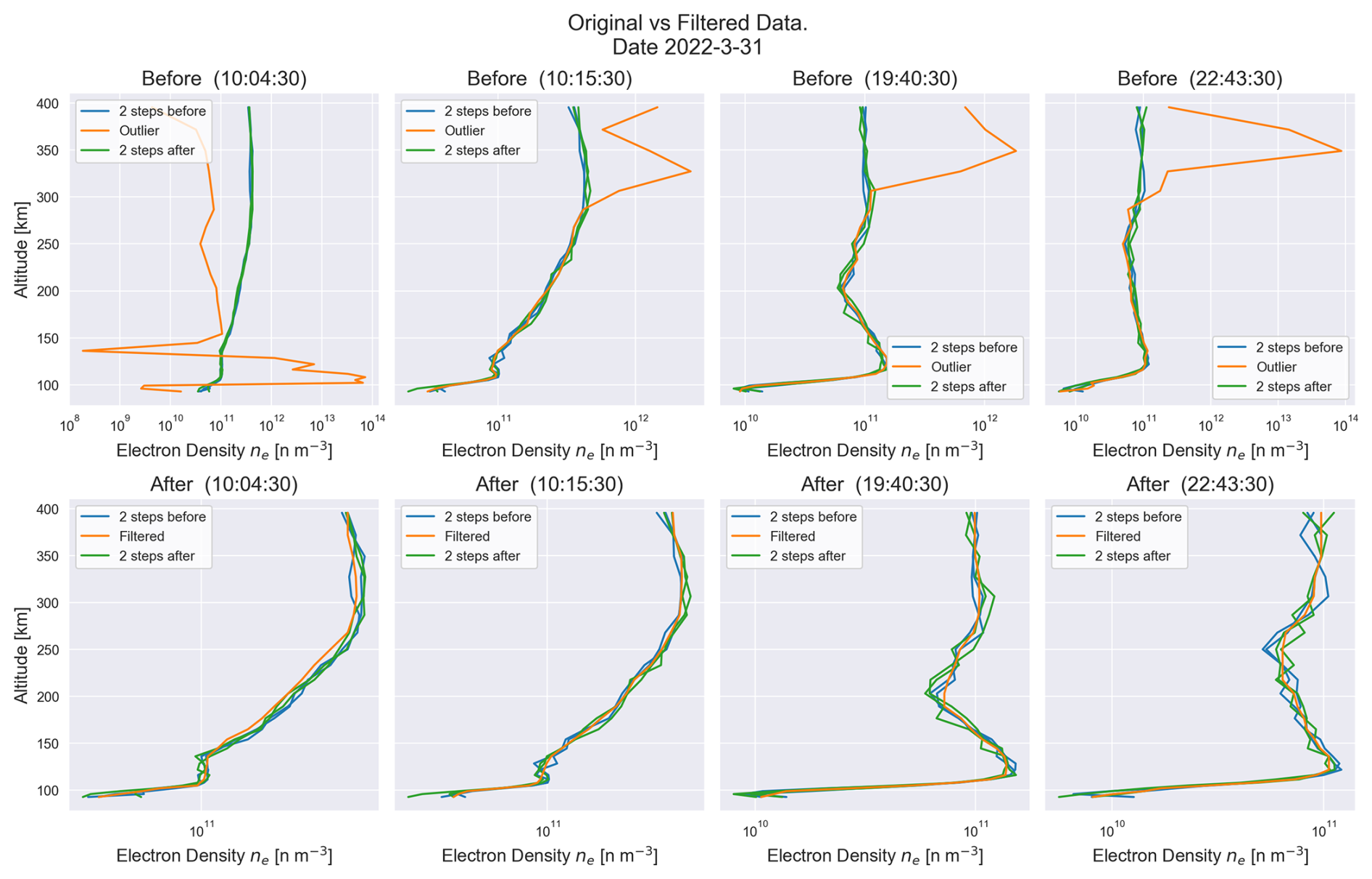
Figure A1 Example of outlier detection and median filtering applied to EISCAT UHF electron-density profiles from 31 March 2022. Each column corresponds to one detected outlier at different measurement times (labeled above each subplot). The top row (“Before”) shows the original profiles, and the bottom row (“After”) shows the profiles after median filtering with kernel = (5 × 5). The y-axis is radar range/altitude (km), and the x-axis is electron density on a logarithmic scale (m⁻³). The orange curve highlights the outlier profile, while the blue and green curves show the profiles from two time steps before and after the outlier, respectively.

Appendix B: Statistical Comparisons of Peak Electron Densities

Given that ARTIST 4.5 demonstrates high accuracy in detecting F-region electron-density peaks, we implemented a peak-identification routine using the find_peaks function from SciPy's signal-processing library. Prominence and related parameters were tuned to capture as many true peaks as possible. E-region peaks were identified within 90–190 km and F-region peaks within 190–350 km. For each model output, the routine records the altitude and magnitude of each detected peak in arrays corresponding to the original profiles. These model-derived peaks were then compared to those observed by the EISCAT UHF radar in a scatter plot (Fig. B1). The performance at peak retrieval was quantified using R², RMSE, and Pearson correlation r_p for each model output.

To assess how well each model captures the overall distribution of peak electron densities, we estimated probability density functions (PDFs) for the E- and F-region peak magnitudes using kernel density estimation (KDE) with a Gaussian kernel (Koutroumbas and Theodoridis, 2008). Similarity between predicted and observed PDFs was quantified via the Bhattacharyya coefficient (BC) (Bhattacharyya, 1943), Jensen–Shannon divergence (JS) (Menéndez et al., 1997), and Wasserstein distance (W) (Villani, 2009), summarized in Table B1. These metrics were chosen to provide a multifaceted evaluation of the agreement between predicted and observed electron density distributions. The BC captures the amount of overlap between the two distributions, providing an intuitive measure of similarity. The JS-div quantifies the similarity between two probability distributions by symmetrizing the Kullback-Leibler divergence (Kullback, 1997), offering a bounded and smoother measure that remains finite even when distributions do not share full support. The W-dist, reflects the minimal effort needed to transform one distribution into the other, giving insight into the overall shape and displacement of the distributions.

For E-region peaks (90–190 km), both KIAN-Net (R²=0.80, RMSE=0.23, r_p=0.90) and Iono-CNN (R²=0.81, RMSE=0.24, r_p=0.91) demonstrate superior performance compared to the baseline models. As shown in Fig. B1(a), Iono-CNN achieves the best peak-distribution alignment with EISCAT UHF peaks (BC=0.99, JS=0.02, W=0.05), slightly outperforming KIAN-Net (BC=0.97, JS=0.10, W=0.12). This indicates that direct ionogram inputs provide marginally higher discriminative power for E-region peak prediction than the fused multi-modal approach. In contrast, ARTIST 4.5 produces mostly constant E-region peak densities around log ₁₀(n_e)≈ 9.2 and some varying clustering below < 10.5, resulting in poor metrics (R² = −4.18, RMSE=0.91, r_p = −0.17) and low distribution similarity (BC=0.64, JS=2.66, W=0.82). E-CHAIM similarly fails to capture E-region variability (R² = −0.04, RMSE=0.56, r_p=0.06), producing quasi-static peaks near log ₁₀(n_e)≈ 10.7 and resulting in a spiked PDF with low similarity (BC=0.25, JS=2.97, W=0.48).

For F-region peaks (190–350 km), all models perform reasonably well. Iono-CNN maintains superior performance (R²=0.91, RMSE=0.12, r_p=0.96), but ARTIST 4.5 slightly outperforms KIAN-Net in peak magnitude estimation (R²=0.89, RMSE=0.11 versus R²=0.87, RMSE=0.14), as summarized in Table B1 and visualized in Fig. B1. This aligns with ARTIST's design focus on F-region Chapman profile modelling from foF2 information within ionograms, though its advantage is restricted to peak magnitudes rather than full-profile accuracy. However, this advantage applies only to peak values and not to full-profile accuracy (Table 3). E-CHAIM shows reduced performance (R²=0.63, RMSE=0.22, r_p=0.81) with a diverging tail forming slightly above log ₁₀(n_e)≈ 11. This is also observed in its F-region probability density function (Fig. B), attributable to systematic underestimation during periods of enhanced ionization on 14 January 00:00 UT and 16 January 2012. This temporal misalignment is reflected in its elevated Wasserstein Distance (W=0.21) compared to KIAN-Net (W=0.08).

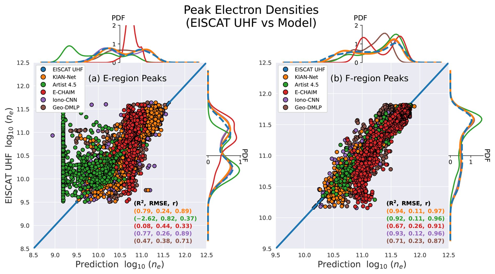
Figure B1 The E- and F-region peak electron densities measured by EISCAT UHF compared to peak predictions made by each prediction/estimation model. The R²-scores together with the RMSE and pearsons correlation r, are plotted in the same order corresponding to the legend. The PDFs are plotted respective to each axis to exhibit the variances in the distributions. (a) Detected E-region peak electron densities for each model plotted along x and y-axes (b) F-region peak electron densities for each model plotted along x and y-axes.

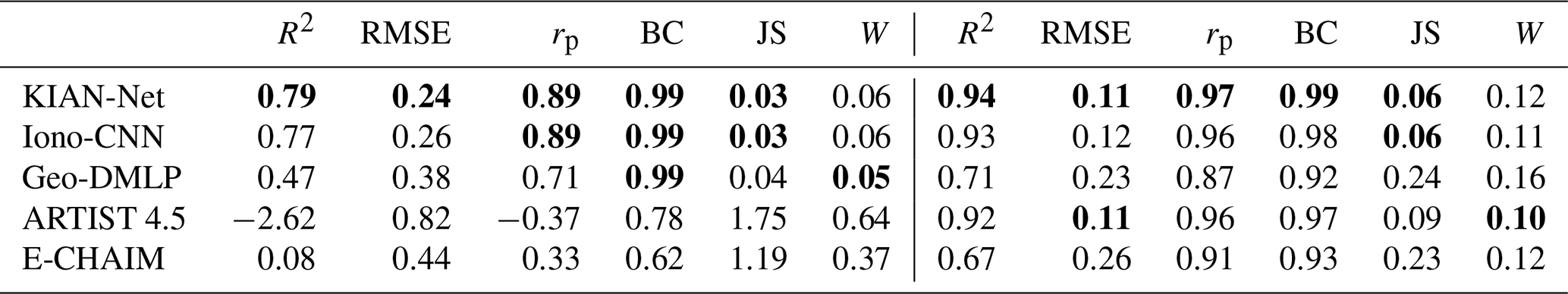
Table B1 Model performance on E- and F-region peak predictions (Fig. B1). Metrics for peak altitudes and magnitudes include R², RMSE, and Pearson correlation (r_p). Distribution similarity metrics for the PDFs are the Bhattacharyya coefficient (BC), Jensen–Shannon divergence (JS), and Wasserstein distance (W). Bold values indicate the best-performance.