Storm-time energy budget in the high latitude lower thermosphere–ionosphere: quantification of energy exchange and comparison of different drivers in TIE-GCM

The energy flow and energy balance in the Lower Thermosphere–Ionosphere (LTI) is governed by a number of processes that are driven by interactions between ions, neutrals and electrons. Even though these processes are well understood theoretically, and even though the framework to implement these processes exists in current global circulation models, the energy estimates for the different processes show large discrepancies between models, in large part because of limitations in available data sets. In this study, we explore numerically the energy inputs and energy transfer between ions, neutrals and electrons during the 2015 St. Patrick's day geomagnetic super-storm. We use NCAR's Thermosphere Ionosphere Electrodynamics General Circulation Model, version 2.0 (TIE-GCM 2.0) for estimating energy sources and sinks, energy transfer rates and the energy partitioning between species. Two independent TIE-GCM runs were executed: the first one used the Weimer 2005 empirical model, and the second used the Assimilative Mapping of Ionospheric Electrodynamics (AMIE) data assimilative technique. The resulting energy budget and the corresponding partitioning of energy between species are inter-compared between the two runs, before and at the peak of the storm. The energy budget is investigated individually for neutrals, ions and electrons, as different heating and cooling mechanisms are associated with each species. Discrepancies between the model runs are discussed and the way forward to close the gaps in present knowledge is highlighted.

1 Introduction

Energy flow in the Earth's Lower Thermosphere–Ionosphere (LTI) is a complex process involving collisional interactions between ions, electrons and neutrals (see, e.g., Sarris et al. (2026) and references therein). A key characteristic of the LTI system is that its energy balance is driven and controlled by external sources of forcing, including solar extreme ultraviolet (EUV) and X-ray irradiance, the solar wind impinging upon the Earth's magnetosphere and energetic particle precipitation. At the same time, upward-penetrating tides and gravity waves continuously deposit energy and momentum from the mesosphere and the troposphere below. During quiet times, or on long-term averages, the main energy input into the LTI is solar radiation, which is absorbed primarily by O₃, O₂, O, CO₂, N₂ and NO (Brasseur and Solomon, 2005). More specifically, O, the most abundant constituent at about 150 km and above, absorbs solar radiation in EUV, O₂ absorbs far ultraviolet radiation (100–200 nm) at altitudes of about 100–150 km, O₃ absorbs solar ultraviolet radiation of 200–300 nm at mid-atmospheric altitudes, and N₂ absorbs radiation ≤ 100 nm at altitudes between 100–200 km. However, during times of enhanced solar and geomagnetic activity, the main energy input into the LTI is energy from the solar wind impinging upon the Earth's magnetosphere, which can greatly exceed the energy input from solar EUV radiation. Furthermore, during active times, energetic charged particles are accelerated in the magnetosphere and precipitate along magnetic field lines into the auroral regions of the LTI. Energetic Particle Precipitation leads to energy deposition, conductivity changes, and chemical changes in the LTI and below, as the braking of precipitating electrons primarily between 90–200 km via collisions with the neutral atmosphere results in increased thermal plasma and heating, and also in enhanced conductivity within this region. During active times, at high latitudes, Joule heating is the most thermodynamically important process, dissipating electromagnetic energy from the magnetosphere. Joule heating greatly affects the state of the LTI by altering neutral winds, temperatures, composition and densities in a significant way. It is thought that, during active times, the effects of Joule heating on the upper atmosphere are more significant than those of EUV or energetic and auroral particle precipitation (e.g., Verkhoglyadova et al., 2016; Knipp et al., 2005). However, the exact quantification of Joule heating is largely unknown, primarily due to a lack of systematic measurements of all relevant terms contributing to Joule heating (see, e.g., Sarris, 2019; Palmroth et al., 2021; Tourgaidis et al., 2025a), leading to large discrepancies between models. It can thus be stated that Joule heating is among the least known and least quantified processes in the LTI, while being among the most significant ones in terms of the energy budget of the ionosphere-thermosphere system, in particular during active times.

Many studies have examined the energy budget of the ionosphere-thermosphere system through model runs of global circulation models. For example, Killeen et al. (1997), performed estimates of the energy budget in the lower thermosphere, using the NCAR Thermosphere–Ionosphere-General Circulation Model (NCAR-TIGCM). They found that LTI heating and cooling has complex morphological dependencies on latitude, longitude, altitude, geomagnetic activity, and season, and they discussed the altitude dependence of each heating term. At the highest altitudes resolved by TIGCM, they found a significant role by minor species chemistry at 175 km, and significant cooling by adiabatic expansion, NO cooling, and downward heat conduction, whereas at 125 km altitude, they found that direct solar insolation and Joule heating are the most important heating terms. Furthermore, they found an equal cooling role of NO and CO₂, with adiabatic expansion being of significance at high latitudes during summer. At 103 km, the lowest altitudes considered, they found that direct solar insolation, heat conduction, and adiabatic compressional effects dominate the heating, whereas the dominant cooling term at these altitudes was caused by CO₂, radiation, with heat advection and adiabatic expansion in the summer hemisphere playing minor roles. Finally, they found that NO cooling rates can double globally during high levels of geomagnetic activity. In another analysis of the LTI energy partition, Verkhoglyadova et al. (2016) used a combination of empirical models and Global Ionosphere-Thermosphere Model (GITM) (Ridley et al., 2006) simulations to investigate the heating and cooling rates in the LTI during two moderate storms caused by High-Speed Streams (HSSs) occurred on 22–31 January 2007 and 25 April–2 May 2011, corresponding to the descending phase of solar cycle 23 and the ascending phase of solar cycle 24, respectively. They used different coupling functions to estimate the energy input from the magnetosphere and consequently they calculated the Joule heating rates using empirical formulations. For the cooling rates, they used data from TIMED/SABER satellite, to derive nitric oxide (NO) and carbon dioxide (CO₂) cooling fluxes. They also performed GITM simulations to cross-compare the model outputs to the satellite derived cooling rates and the heating rates based on empirical estimations. For the external driving of the model, they used the Weimer-2005 and the AMIE formulation for defining the high latitude electric fields. By comparing the GITM outputs to the satellite and empirical data, they found that GITM consistently underestimates NO cooling and auroral heating. Furthermore, Verkhoglyadova et al. (2017), calculated the energy budget of the ionosphere-thermosphere for the storms of March 2013 and 2015 using the GITM model together with observational proxies. GITM was driven by solar wind data, the F10.7 index, the OVATION Prime model and the Weimer 2005 model. They found that Joule heating and infrared cooling are likely underestimated in GITM. Despite of significant modeling and observational efforts, the relative contributions from different external drivers to the energy budget in LTI is still a subject of debate, hindering efforts to forecast the state of the LTI, in particular during times of enhanced solar and geomagnetic activity (Heelis and Maute, 2020). At the same time, various mechanisms internal to the LTI convert, transport and redistribute the input energy from the system. Whereas these mechanisms are well-understood theoretically, their quantification also yields large discrepancies between different models.

In this paper, we present model results on the quantification of the various energy dissipation terms in the LTI during the geomagnetic storm of St. Patrick's day 2015, as estimated through a simulation using TIE-GCM. Through these simulations, we compare the magnitudes of the hemispherically-integrated heating and cooling terms during the evolution of the storm. In particular, we use two different common models of external driving of the LTI system, an empirical and an assimilative model, and we compare their effects on the energetics and overall energy budget of the LTI. In further detail: in Sect. 2.1 we present an overview of the St. Patrick's day 2015 geomagnetic storm and studies that have reported observations and modeling results of that event; in Sect. 2 we describe the TIE-GCM and the simulations that were conducted; and in Sect. 2.3 we present in more detail the two different models that are used in this study as external drivers for TIE-GCM to perform the three energy budget inter-comparisons. In Sect. 3 we describe the estimation methodology and the formulation that is used to calculate each heating and cooling term, listing the relevant TIE-GCM geophysical observables. In Sect. 4 we present the main results and inter-comparisons, estimated from the point of view of the neutrals, the ions and the electrons. In Sect. 5 we discuss the results of the simulations, and in Sect. 6 we summarize the main findings and conclusions of this study.

2 TIE-GCM simulation of St. Patrick's day storm

2.1 St. Patrick's day storm

On 17 March 2015, a severe geomagnetic storm of G4 class was recorded, reaching a minimum Dst index of approximately −223 nT. Known as the 2015 St. Patrick's Day storm, it was the strongest G4 event during Solar Cycle 24, one of only five such storms observed. The storm was triggered by a coronal mass ejection (CME) that occurred around 02:00–02:30 UT on 15 March. An interplanetary shock associated with this CME was detected by the Wind spacecraft at approximately 03:59 UT on 17 March. The onset of the geomagnetic storm at Earth was recorded near 14:00 UT, lasting roughly 18 h, with G3/G4 level geomagnetic conditions sustained for about 12 h. A minimum Dst of -223 nT was reached at approximately 23:20 UT. A detailed description of the storm can be found in Wu et al. (2016), and references therein. Due to its severity, this event has been extensively investigated: for example, Lyons et al. (2016), Prikryl et al. (2016), and Marsal et al. (2017) studied energy inputs into the high-latitude regions during this event, focusing on the ionospheric disturbances induced by these energy inputs. Yue et al. (2016), Zhang et al. (2017) and Wei et al. (2019) investigated the observed sub-auroral processes and the related coupling between the ionosphere and the magnetosphere. Zakharenkova et al. (2016) and Dmitriev et al. (2017) studied the response of the neutral winds to the high-latitude energy and momentum inputs and the effects that the storm had on neutral wind patterns. Goldstein et al. (2017) studied ring current dynamics and the enhancement of the plasmasphere. Kanekal et al. (2016) and Hudson et al. (2017) reported the prompt injection and acceleration of energetic electrons. Jaynes et al. (2018) and Ozeke et al. (2020) investigated ULF-driven radial diffusion during this event. Tourgaidis et al. (2025a) calculated the Joule heating rates during this event, using two of the most commonly used physics-based Global Circulation Models (GCM) of the Earth's upper atmosphere: the Global Ionosphere/Thermosphere Model (GITM) and the Thermosphere–Ionosphere-Electrodynamics General Circulation Model (TIE-GCM), as well as empirical models, and performed detailed comparisons between the various model runs.

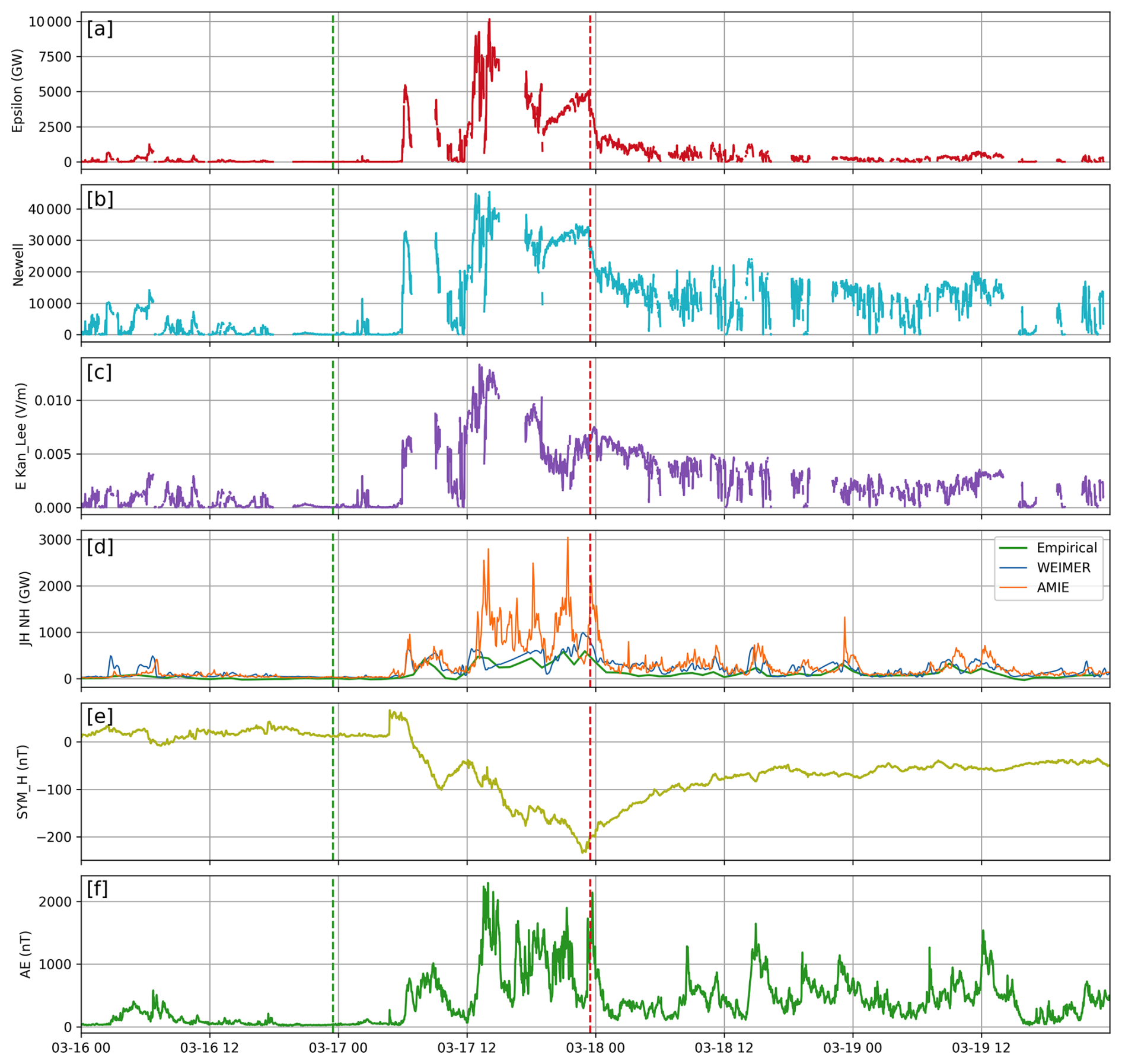
Figure 1 Description of the geomagnetic storm through various parameters: (a) Akasofou ϵ parameter, (b) Newell coupling function, (c) Kan–Lee electric field, (d) Joule heating estimates (Empirical, TIE-GCM Weimer, TIE-GCM Amie), (e) SYM-H index (f) AE index. The red dashed vertical line marks the time of minimum SYM-H index, indicating the peak of the storm. The blue dashed vertical line corresponds to 24 h before the peak of the storm.

An overview of the time evolution of all key parameters relevant to the coupling of the Magnetosphere-Ionosphere-Thermosphere system during this event are presented in Fig. 1. The Akasofu ϵ parameter (Akasofu, 1981), plotted in Fig. 1a, is a measure of the solar wind energy input into the magnetosphere. It is given as:

$$\begin{array}{}\text{(1)}& \mathit{ϵ}=V_{\text{sw}}{B}^{\mathrm{2}}{\sin }^{\mathrm{4}}(\mathit{\theta }/\mathrm{2})l_{\mathrm{0}}^{\mathrm{2}}\end{array}$$

where V_sw is the solar wind speed, B is the interplanetary magnetic field magnitude, $\mathit{\theta }={\tan }^{-\mathrm{1}}(B_y/B_x)$ is the IMF clock angle and l₀ is the characteristic length scale of the magnetopause (≈ 7 R_e). The Newell coupling function (Newell et al., 2007), plotted in Fig. 1b, is an empirical formula representing the efficiency of solar wind–magnetosphere coupling:

$$\begin{array}{}\text{(2)}& \mathrm{\Phi }=V_{\text{sw}}^{\mathrm{4}/\mathrm{3}}{B}_{\mathrm{T}}^{\mathrm{2}/\mathrm{3}}{\sin }^{\mathrm{8}/\mathrm{3}}(\mathit{\theta }/\mathrm{2})\end{array}$$

The Kan–Lee electric field (Kan and Lee, 1979), plotted in Fig. 1c, describes the magnetospheric convection electric field as it maps down to the high latitude ionosphere, giving a description of how energy from the solar wind enters the Earth's magnetosphere and ionosphere. Is expressed as:

$$\begin{array}{}\text{(3)}& E_{\text{KL}}=V_{\text{sw}}{B}_{\mathrm{T}}{\sin }^{\mathrm{2}}(\mathit{\theta }/\mathrm{2})\end{array}$$

where $B_{\mathrm{T}}=\sqrt{B_y^{\mathrm{2}}+B_x^{\mathrm{2}}}$ is the transverse component of the interplanetary magnetic field (IMF). The SYM-H index, plotted in Fig. 1e, is a high-resolution (1 min) analog of the Dst (Disturbance storm-time) index, and it represents the strength of the symmetric ring current around Earth. It is used to monitor geomagnetic storm activity with finer temporal resolution than Dst. The AE index (Auroral Electrojet index), plotted in Fig. 1, quantifies the intensity of auroral zone currents, specifically the eastward (EEJ) and westward (WEJ) electrojets. It is a key indicator of auroral and substorm activity, primarily reflecting variations in the Earth's high-latitude magnetic field caused by enhanced ionospheric currents. The Joule heating deposited onto the ionosphere-thermosphere during this time, calculated via an empirical formulation according to Knipp et al. (2005), is plotted in Fig. 1d. This is given as:

$$\begin{array}{}\text{(4)}& \text{JH}=\mathrm{29.41}\text{PC}+\mathrm{2.54}{\text{PC}}^{\mathrm{2}}+\mathrm{0.21}\text{Dst}+\mathrm{0.0023}{\text{Dst}}^{\mathrm{2}}\end{array}$$

where PC and Dst are the Polar Cap and Disturbance Storm Time indices, respectively. Together with the empirical formulation of Joule heating according to Knipp et al. (2005), in Fig. 1d we also plot the Joule heating rate calculated through TIE-GCM runs driven by the Weimer and AMIE models; these will be discussed in more detail in the following.

From the panels in Fig. 1 it can be seen that the SYM-H index becomes negative on 17 March, 06:53:00 UT, subsequently it presents a local minimum of −101 nT at 09:37:00 UT, another local minimum of −177 nT at 17:28:00 UT, and it reaches its minimum value of −234 nT at 22:47:00 UT. Subsequently, SYM-H keeps increasing after the peak of the storm while it continues to be negative for the next 4 d. The ϵ parameter, which is an estimation of the total power extracted from the solar wind/Interplanetary Magnetic Field into the magnetosphere, presents its first sharp rise to 5453 GW at 06:14:00 UT, its maximum value of 10157 GW at 14:06:00 UT, while around the minimum of the SYM-H index has an elevated value of around 5000 GW. Following on, its values drop rapidly and become comparable to the pre-storm period. The Newell coupling function and the Kan–Lee electric field follow the same trend as the ϵ parameter, with the difference that their values remained elevated after the storm, with respect to the pre-storm period. The Joule heating estimations through the Knipp et al. (2005) empirical formula and with the Weimer driver, are in good agreement, while there are large differences between these model results and the Joule heating as calculated by the AMIE run. Finally, regarding the AE index, there are many local maximums during the main phase of the storm and it has high correlation with the Joule heating calculated with the AMIE run. For the following analyses, we chose the time of the peak of the AMIE Joule heating which is closest to the minimum of the SYM-H index, i.e. at 23:30:00 UT of 17 March, marked with a dashed vertical red line in Fig. 1. As a pre-storm baseline timestep we chose one day before, i.e. at 23:30:00 UT of 16 March marked with a dashed blue line. It is noted that the interplanetary coupling functions ϵ, the Newell parameter and the Kan–Lee electric field include gaps in their timeseries resulting from data gaps of the interplanetary magnetic field measurements.

In this paper, using TIE-GCM (see Sect. 2), we simulate 4 d around the St. Patrick's day storm, starting from 2 d before and up to 2 d after the time of the minimum Dst index of the event, and we quantify the various energy sources and energy dissipation terms in the Lower Thermosphere–Ionosphere. Energy terms are viewed from the perspective of the neutrals, the ions and the electrons, allowing to monitor the energy transfer between species. We use two different electric potential models as external drivers to TIE-GCM (see Sect. 2.3), and we quantify and cross-compare the variations in the various energy terms based on the different external drivers.

2.2 The Thermosphere–Ionosphere – Electrodynamics General Circulation Model (TIE-GCM)

A global self-consistent simulation of the LTI environment during St. Patrick's day stom was performed using the National Center for Atmospheric Research (NCAR) Thermosphere–Ionosphere-Electrodynamics General Circulation Model (TIE-GCM). TIE-GCM is a three-dimensional global model of the thermosphere and ionosphere system, spanning altitudes from ∼ 100 up to ∼ 600 km. TIE-GCM is based on first-principles and, at each simulation time step, solves the momentum, energy and continuity equations for neutral, ion and electron species. In this study, version 2.0 of the TIE-GCM is used in the simulations.

Calculations of the various energy terms were performed at every grid point of TIE-GCM; as the focus of the study is the high latitude LTI, energy terms were integrated from 56° latitude up to the pole, and across all longitudes and altitudes. The TIE-GCM grid is pressure defined, thus in order to perform the integration a re-griding procedure was followed to translate the pressure defined grid to altitude defined. After the re-griding procedure, integrations were performed with a trapezoidal integration scheme, according to equation:

$$\int f\left(x\right)\approx \sum \left(\right[f\left(x_{k-\mathrm{1}}\right)+f\left(x_k\right)]/\mathrm{2})\times \mathrm{\Delta }x$$

The TIE-GCM uses an imposed electric field model as external driver for the specification of the electric potential at high magnetic latitudes. Two such models are used in this study, and the results from the two runs are inter-compared, as the external specification significantly affects the resulting energy flow. These external drivers are described in further detail in the following section.

2.3 External drivers of TIE-GCM – Electric Potential and Particle Precipitation Models

The thermosphere–ionosphere system is driven externally by high-latitude electric fields as well as auroral precipitation. TIE-GCM is correspondingly driven by models that provide specifications of high-latitude electric fields and particle precipitation. In this study, two different models are used, namely, the Weimer-2005 empirical model (Weimer, 2005), and the Assimilative Mapping of Ionospheric Electrodynamics (AMIE) procedure developed by Richmond and Kamide (1988). The Weimer-2005 empirical model of high-latitude ionospheric electric potential utilizes upstream solar wind and geomagnetic parameters to reconstruct convection patterns. The model is based on measurements of electric fields by the Dynamics Explorer 2 (DE-2) and the Defense Meteorological Satellite Program (DMSP) satellites. Model inputs include the interplanetary magnetic field (IMF) components B_x, B_y, and B_z, as well as the solar wind velocity V_x, which controls the strength of the convection. Additionally, the model incorporates the geomagnetic dipole tilt angle and universal time (UT) to account for seasonal and diurnal asymmetries in the potential pattern. Unlike models based on geomagnetic indices such as Kp or Dst, the Weimer model derives directly from solar wind conditions, enabling a more physically driven and hemispherically resolved specification of ionospheric electrodynamics (Weimer, 2005). This model offers higher spatial resolution and better IMF sensitivity than earlier empirical models like the Heelis et al. (1982) and the Weimer-2001 models. The Assimilative Mapping of Ionospheric Electrodynamics (AMIE) (Richmond and Kamide, 1988) model is a physics-based, data assimilative technique that produces time-dependent maps of high-latitude ionospheric electrodynamics. It assimilates diverse ground (ground magnetometers, ionospheric radars, incoherent scatter radars) and space-based observations. In addition to convection maps, AMIE provides conductivity, as well as ionospheric and field-aligned current estimations in a self-consistent physics-based framework.

It is noted that in the AMIE-driven simulation both the high-latitude electric potential and the auroral precipitation are derived from the AMIE solution, ensuring internal consistency between the electrodynamics and particle energy input. In contrast, in the Weimer-driven simulation, the electric potential is specified using the statistical Weimer (2005) model, while auroral precipitation is prescribed using an empirical parameterization based on the IMF Bz and By, and the solar wind velocity (see TIEGCM 2.0). Thus, the convection and precipitation forcing in the Weimer-driven simulation are not derived from a single electrodynamic solution but represent independent statistical descriptions. This difference in forcing consistency may contribute to differences in the simulated energy deposition and thermospheric response, particularly during the peak of the storm.

3 Estimation Methodology

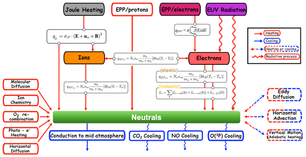
The energy state and energy balance of the LTI is determined by a number of processes that result in the storage, transport, and transformation of energy into various forms. These processes are governed by collisional interactions between species that determine the energy transfer between ions, neutrals and electrons, as well as by radiative heating due to EUV radiation and radiative cooling due to species such as CO₂, NO and O(³P). A schematic diagram of the energy flow and the associated processes and pathways in the LTI system is given in Fig. 2. In this figure, the transfer of energy towards and between the neutral species, ionized species and electrons of the thermosphere–ionosphere system is shown with arrows, as marked. These processes include: Joule heating, which is deposited to the neutrals and the ions; energy deposition from energetic precipitating protons, which deposit energy directly to the neutrals; energy deposition from energetic precipitating electrons, which deposit energy to the ionospheric electrons; EUV radiation, considered the most significant energy source during quiet times, which heats both the electrons and the neutrals; heat exchange due to temperature differences between: ions and neutrals, ions and electrons, electrons and neutrals; molecular diffusion at higher altitudes; chemical processes related to ion chemistry; heating due to O₂ recombination; photoelectron heating; horizontal diffusion; eddy diffusion, occurring primarily at regions closer to the mesosphere; horizontal advection; and adiabatic heating due to the vertical motion of neutral gases. The most significant radiative cooling terms in the thermosphere include CO₂ and NO, and to a smaller extent O(³P). Finally, a cooling term is conduction to the middle atmosphere. The processes that are calculated in TIE-GCM are marked with boxes having a solid outline, whereas processes that are not calculated and are thus not presented herein are marked with dashed outlines.

Figure 2 Energy flow in the Lower-Thermosphere–Ionosphere system.

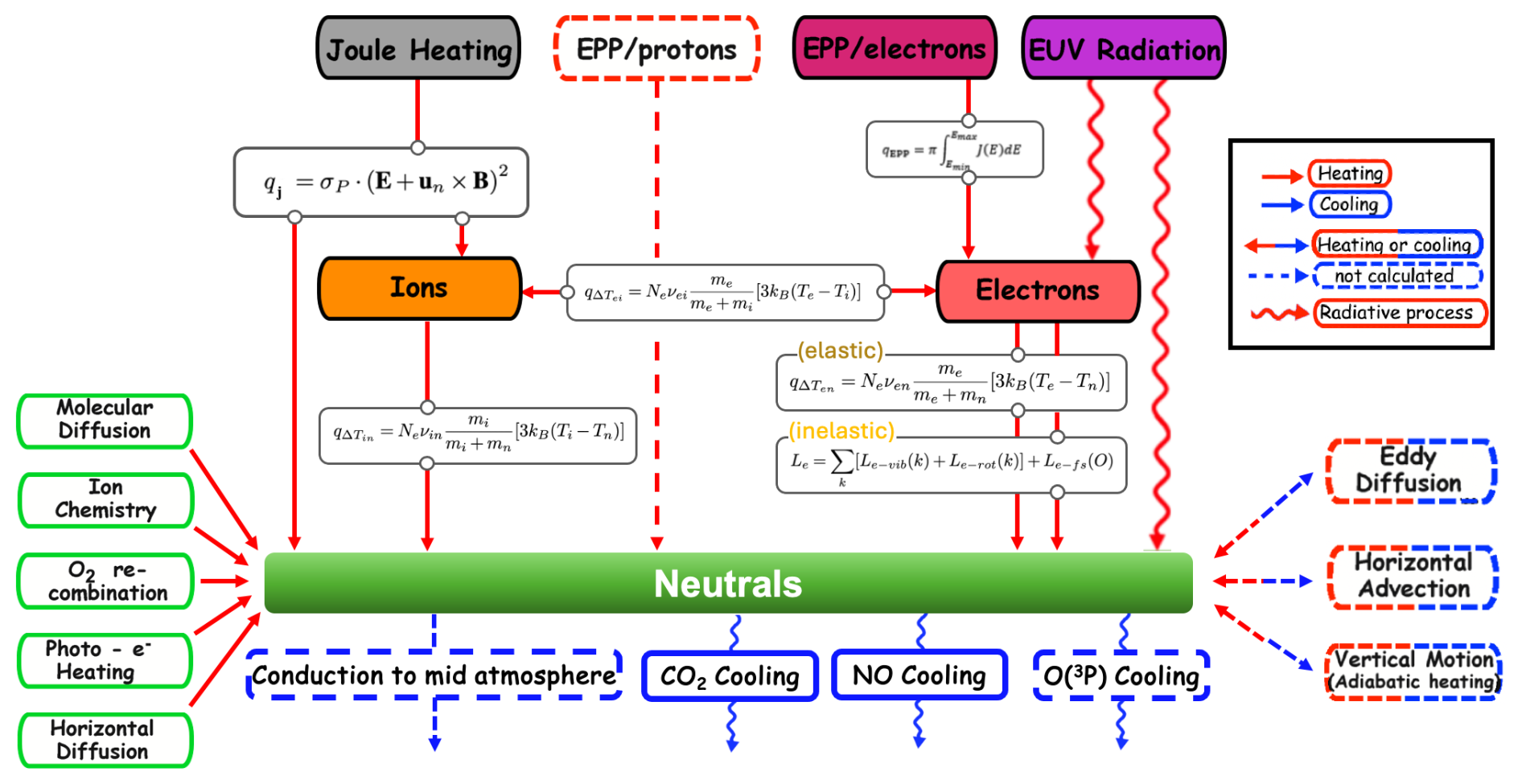
In this study, TIE-GCM is used to estimate numerically each of the energy flow process shown in Fig. 2. In brief, these processes include external heating processes, energy transfer between the neutrals, ions and electrons, and heating or cooling of the neutrals due to various other Thermosphere processes. External heating processes include Joule heating, which is deposited to the neutrals either promptly during active times, or indirectly through the initial heating of the ions and the subsequent energy exchange between ions and neutrals; Energetic Particle Precipitation, including energetic protons, which deposits energy directly to the neutrals, and energetic electrons, which ionize the neutral particles and create photoelectrons which subsequently get thermalized; solar extreme ultraviolet (EUV) radiation, which is the most significant heating energy source in the LTI, on long-term averages. Energy transfer can occur from the ions to the neutrals, between ions and electrons, and from the electrons to the neutrals. Finally, other neutral heating processes include molecular diffusion, ion chemistry, O₂ recombination, photo-electron heating, horizontal diffusion; eddy diffusion, horizontal advection and adiabatic heating, which can lead to either heating or cooling; radiative cooling from CO₂, NO and O(³P); and cooling due to conduction to the middle atmosphere. Each of the processes shown in this figure is discussed in more detail in the following section. The equations used and the overall estimation methodology are based on Daedalus MASE (Mission Assessment through Simulation Exercise) (Sarris et al., 2023b), which is an open-source package of scientific analysis tools aimed at research in the Lower Thermosphere–Ionosphere (LTI). Daedalus MASE was created with the purpose to assess the performance and demonstrate closure of the mission objectives of Daedalus (Sarris et al., 2020), a mission concept targeting to perform in-situ measurements in the LTI. However, through its successful usage as a mission-simulator toolset, Daedalus MASE has evolved to encompass numerous capabilities related to LTI science and modeling.

The calculations of the energy transfer and energy dissipation terms are based on calculations of a comprehensive list of geophysical parameters (or physical quantities) of the LTI, which are obtained through a TIE-GCM simulation of the solar storm of St. Patrick's day, March 2015. These geophysical observables include: (a) Plasma (ionosphere) parameters: Ion Drift velocity vector (v_i), Ion Temperature (T_i), Electron Temperature (T_e), Ion Number Density (N_i), Electron Number Density (N_e), Ion Composition (n_ix); (b) Neutral (thermosphere) parameters: Neutral Wind Velocity vector (u_n), Neutral Mass Density (ρ), Neutral Temperature (T_n), Neutral Composition (n_nx), and (c) LTI fields: the Magnetic Field vector (B), and the Electric Field vector (E). In the following section, each of the energy flow terms of Fig. 2 is described in further detail, including an overview of the theory and the main assumptions that are used in their derivation in TIE-GCM.

3.1 Heating and Cooling Rates

3.1.1 Joule heating

Joule heating is a major heat dissipation process in the LTI, particularly during active times. Joule heating is caused by collisions between ions and neutrals in the presence of a relative drift between the two (Vasyliūnas and Song, 2005). Ion-neutral collisions tend to drive the neutral gas in a similar convection pattern to that of the ions, which with time also generates kinetic energy (Codrescu et al., 1995; Richmond, 1995). The Joule heating estimation methodology based on TIE-GCM outputs is discussed in further detail in Tourgaidis et al. (2025a), who simulated Joule heating during several days around the superstorm of St. Patrick's day, 2015. Generally, Joule heating is deposited promptly into the neutral gas and also heats the ions. In turn, the ions are transferring heat to the neutral gas, as is further discussed below. The Joule heating rate per unit volume, q_Joule, is derived as:

$$\begin{array}{}\text{(5)}& q_{\mathrm{J}}={\mathit{\sigma }}_P\cdot (\mathit{E}+{\mathit{u}}_{\mathrm{n}}\mathrm{\times }\mathit{B}{)}^{\mathrm{2}}\end{array}$$

where σ_P is the Pedersen conductivity, E is the electric field vector, u_n is the neutral wind velocity vector, and B is the magnetic field vector. The dependence of Joule heating on the neutral wind is introduced here because the electric current that results in this heating is passing through the moving neutral gas in a way that the electric field of consequence to heating will depend on its vector in relation with that moving media. Joule heating is deposited to the neutrals either promptly, or through the heating of the ions and the subsequent energy exchange between the ions and neutrals, due to their difference in temperature. Due to the limited spatial resolution of Global Circulation Models such as TIE-GCM and GITM, only large-scale electric field structures are captured. On the other hand, it is known that sub-grid small scale electric field structures have a very significant impact to the amount of Joule heating, especially during geomagnetic storms (see, e.g. Matsuo and Richmond, 2008). To account for this, in TIE-GCM, the Joule heating rate, deposited to the neutrals, is multiplied by default by a factor of 1.5. However, as discussed by, e.g., Baloukidis et al. (2023), there are still many unknowns concerning the value that should be used as a function of altitude, solar activity and magnetic local time, leading to large discrepancies between models. These discrepancies and their potential sources have been explored in further detail by Tourgaidis et al. (2025a).

3.1.2 Energetic Precipitating Electrons

Energetic electron precipitation is another heating source in the LTI. Together with Joule heating, energetic particle precipitation passing through the LTI has profound effects on conductivity within this region, and significantly influences chemistry at altitudes below. Electron precipitation also contributes significantly to the observed electron density in the LTI (Verronen et al., 2015). Within the LTI, energetic precipitating electrons mainly ionize the neutral particles, and this also heats the electrons as the newly created electrons (photoelectrons) get thermalized. It is known through simulations that precipitating electrons with energies greater than ∼ 200 keV deposit their energy below the D-region ionosphere, at altitudes below ∼ 70 km, altering the chemistry of the neutral atmosphere and contributing to ozone destruction through the production of HO_x and NO_x. Precipitating electrons with energies of the order of 10 to 100 keV deposit their energy within the D and E region, at altitudes of approximately 70 to 120 km (e.g., Fang et al., 2008; Turunen et al., 2009; Miyoshi et al., 2010; Tesema et al., 2020), altering the chemical and electrical properties of the region and contributing to changes in conductivity and heating. Electrons of energies on the order of or below 1 keV deposit energy to the F region, causing electron density variations. A smaller fraction of the precipitating particle energy flows directly to the neutral gas, particularly via proton precipitation. However, due to a lack of detailed measurements of energetic proton precipitation, this energy fraction is not fully quantified. Electrons above energies of 10 keV provide a significant energy input into the LTI, while electrons above energies of 50 keV can have significant consequences in the chemical composition of the LTI and below, as they ionize neutrals in a series of chemical reactions that result in the production of H, OH and HO₂, which are termed collectively odd hydrogen, or HO_x, and N, NO and NO₂, which are termed collectively odd nitrogen, or NO_x; These are known to subsequently lead to the catalytic destruction of ozone (Randall et al. (2007).

Electron precipitation is typically caused by a variety of wave-particle interaction mechanisms (e.g., Chorus, Hiss, EMIC etc), which are well modeled and understood theoretically, albeit with significant quantitative uncertainties. These mechanisms have been well described theoretically and have been modeled in detailed wave-particle interaction codes (see, e.g., the comprehensive wave–particle interaction tool-set of models, in Tourgaidis and Sarris (2022), and references therein). Also, the effects of Energetic Precipitating Electrons have been implemented in chemistry-climate models that extend from the surface up to LTI altitudes (see, e.g., Verronen et al., 2016). The equation for the energy flux due to electron precipitation, is given as:

$$\begin{array}{}\text{(6)}& q_{\text{EPP}}=\mathit{\pi }\underset{E_{min}}{\overset{E_{max}}{\int }}J\left(E\right)\mathrm{d}E\end{array}$$

where J(E) is the differential energy flux as a function of energy and E_min and E_max are the lower and upper bounds of electron energy contributing to precipitation. However, there are still significant open questions regarding the impacts of EPP. For example, the formation rates of the various NO_x species that are attributed to energetic particle precipitation are currently not known. Furthermore, the coupling between chemical changes, atmospheric heating and cooling rates, and atmospheric dynamics is still an open question (Sinnhuber et al., 2012). Related to the energy balance and energy deposition in the LTI, a key open question is related to the thermal efficiency of the EPP heating. This is still an open question, as the collision cross-section of precipitating electrons with neutral species is energy dependent. This means that higher energy particles will have smaller collision cross-sections with the neutrals. Thus, higher energy particles are able to penetrate deeper into the atmosphere. At lower altitudes, inelastic collisions become significant, and the kinetic energy of the electrons is converted to thermal energy with higher efficiency. This thermal efficiency is known to be dependent on the particle kinetic energy and consequently on altitude in the LTI, but it is poorly known.

3.1.3 Energetic Precipitating Protons

Energetic proton precipitation is caused either by adiabatic loss when ions are transported toward Earth and experience widened loss cones, by the resonant interactions with EMIC waves, or by pitch angle diffusion due to increased field-line curvature radius. Energetic Precipitating Protons can be a significant source of heating of the neutrals in the LTI. Protons in the keV energy range deposit most of their energy in the E region, at altitudes between 100 and 160 km, whereas MeV proton energy deposition occurs at lower altitudes, typically in the D region and below (Galand, 2001). They impact the neutrals directly, and can be more significant at certain locations and times, such as the equatorial edge of the evening auroral oval (Galand et al., 2001). Energetic proton precipitation is generally considered to play a secondary role in affecting the LTI compared to energetic electron precipitation, since the ions usually carry lower energy flux and contribute less to the ionization of the upper atmosphere. This is due to the larger mass and shorter mean free path of protons in the lower thermosphere. Nevertheless, it has been found that, at times, proton precipitation can dominate over electrons in some regions; furthermore, studies have shown that medium-energy (10s of kev) precipitating protons can carry more energy flux than electrons (Tian et al., 2020), providing substantial energy deposition down to the ionosphere. At the same time, proton precipitation can lead to significant enhancements in the conductance (Galand and Richmond, 2001; Zou et al., 2014), and can distort the potential pattern in the LTI (Khazanov et al., 2003). As a conclusion, although it is secondary to the electron precipitation, the proton precipitation is still important (Newell et al., 2009), as, at times, it can be a major energy source, and thus a key contributor to auroral emission. Solar proton precipitation inside the polar cap is included in TIEGCM, with a characteristic energy in the default model configuration that is assumed to be 10 keV and an energy flux that is set to a very low default value (1 × 10⁻²⁰). A realistic and time-variable proton precipitation is an improvement that needs to be incorporated in future model runs.

3.1.4 Solar Radiation Heating

During quiet solar and geomagnetic conditions, solar UV Radiation is the most significant heating energy source in the LTI, leading to a significant increase in neutral temperatures in the thermosphere. In particular, solar extreme ultraviolet radiation, EUV and soft X rays are absorbed at altitudes above 90 km and lead to the ionization of the major LTI neutral species, N₂, O, and O₂, and to the creation of the ionosphere. EUV radiation and leads to the dissociation of the molecular species through direct photo-dissociation and to many indirect processes driven by ionization, the most important of which is the generation of energetic electrons. These electrons carry the excess energy that is transferred by photoionization, and lead to further ionization, dissociation, and excitation of the neutral constituents, and to a chain of elastic and inelastic processes that transfer the EUV radiation energy into the thermosphere and ionosphere.

Electrons are also heated by ionizing UV radiation. The resulting thermal energy is transferred from electrons to neutrals and ions. UV radiation is the strongest heating source on a global scale. By measuring the ratio of $T_{\mathrm{e}}/T_{\mathrm{n}}$, which is driven by EPP and UV radiation, it is possible to estimate the fraction of UV radiation that is deposited to the electrons and neutrals. However, it is noted that, similarly to T_i and T_n, co-temporal and co-spatial measurements of T_e and T_n are extremely rare.

There are several missions that have been providing long-term, high-resolution spectral irradiance measurements that have been used for calculating the ionization and dissociation rates in the thermosphere, and for providing the inputs for solar irradiance models. These, in turn, are standard inputs for general circulation models of the thermosphere and ionosphere, such as TIE-GCM. However, there are significant uncertainties related to the photoelectrons that are generated by ionization, which lead to further ionization and dissociation of the neutrals in the thermosphere. Furthermore, the deposition of solar EUV energy in the thermosphere is strongly dependent on both wavelength and altitude, peaking in the 100 to 200 km altitude range, and dropping sharply right below (see, e.g., Fig. 1b of Solomon and Qian, 2005).

More specifically, solar extreme ultraviolet (EUV) irradiance in TIE-GCM is specified using the EUVAC model (Richards et al., 1994) in the range 5–105 nm. EUVAC is based on the F74113 reference spectrum, measured during low solar activity, with adjustments applied in specific wavelength ranges (e.g., fluxes between 15–25 nm doubled and fluxes below 15 nm increased by a factor of three). Solar variability is parameterized using the F10.7 index (daily and 81 d average values). For wavelengths < 5 nm, GOES X-ray measurements are used to establish reference irradiance and variability. The 1.8–5 nm range follows the Hinteregger model (Hinteregger, 1981) based on the SC21REFW spectrum, while the 105–175 nm range is specified using the Woods and Rottman model (Woods and Rottman, 2002) derived from UARS/SOLSTICE observations.

3.1.5 Transfer of energy between species due to elastic collisions

In the presence of collisions between the ions, neutrals and electrons, a transfer of energy will occur that will be dependent upon the temperature difference between the species, the collision frequency and the total plasma density. In the LTI, electron temperatures are expected to always be higher than ion temperatures which, in turn, should be higher than neutral temperatures, namely $T_{\mathrm{e}}>T_{\mathrm{i}}>T_{\mathrm{n}}$. Thus, the ions are generally cooled by the transfer of heat to the neutral gas when the temperature of the ions, T_i is larger than the temperature of the neutrals, T_n (T_i>T_n). Similarly, the electrons are expected to have higher temperatures than the ions, leading to a heat transfer from the electrons to the ions. The ion-neutral heat transfer rate is given by:

$$\begin{array}{}\text{(7)}& q_{\mathrm{\Delta }{T}_{\text{in}}}=N_{\mathrm{i}}{\mathit{\nu }}_{\text{in}}{\displaystyle \frac{m_{\mathrm{i}}}{m_{\mathrm{i}}+m_{\mathrm{n}}}}\left[\mathrm{3}{k}_B\right(T_{\mathrm{i}}-T_{\mathrm{n}}\left)\right]\end{array}$$

where ν_in is the ion-neutral collision frequency (see Eq. 14 in Sarris et al., 2023b). Thus, simultaneous measurements of T_i and T_n together with knowledge of the ion-neutral collision frequency are needed for the estimation of the heat transfer rate from ions to the neutrals and its comparison with Joule heating rates. Such simultaneous measurements of T_i and T_n are extremely rare, and have only been made for a very limited amount of time by the Atmosphere Explorers AE-C and AE-E in the late 70s and early 80s (see, e.g., Fig. 11 of ESA-Daedalus-RfA, 2020), leading to large uncertainties and to a lack of quantitative understanding of the state of thermal equilibrium of the LTI. This has been highlighted by Peterson et al. (2023), who analyzed simultaneous electron, ion and neutral temperature measurements from AE-C below 140 km, together with remote sensing observations over the Millstone Hill Incoherent Scatter Radar, and demonstrated events where the condition $T_{\mathrm{e}}>T_{\mathrm{i}}>T_{\mathrm{n}}$, does not always hold true. They left open the potential of uncertainties in our quantification and understanding of processes in the LTI, highlighting the need for new measurements. The relative temperatures of ions and neutrals were further studied statistically by Pirnaris and Sarris (2023), who showed that there is a significant percentage of times where the condition $T_{\mathrm{e}}>T_{\mathrm{i}}>T_{\mathrm{n}}$ does not hold true, and pointed to the possibility of missing physics and quantitative understanding in the LTI. In TIE-GCM code, the T_i≥T_n condition is imposed and is always true.

Similarly to the ion-neutral heating rate, the electron-ion heating transfer rate due to electron-ion collisions is calculated according to:

$$\begin{array}{}\text{(8)}& q_{\mathrm{\Delta }{T}_{\text{ei}}}=N_{\mathrm{e}}{\mathit{\nu }}_{\text{ei}}{\displaystyle \frac{m_{\mathrm{e}}}{m_{\mathrm{e}}+m_{\mathrm{i}}}}\left[\mathrm{3}{k}_B\right(T_{\mathrm{e}}-T_{\mathrm{i}}\left)\right]\end{array}$$

where ν_ei is the electron-ion collision frequency (see Eq. 15 in Sarris et al., 2023b). Finally, the electron-neutral heat transfer rate is given by:

$$\begin{array}{}\text{(9)}& q_{\mathrm{\Delta }{T}_{\text{en}}}=N_{\mathrm{e}}{\mathit{\nu }}_{\text{en}}{\displaystyle \frac{m_{\mathrm{e}}}{m_{\mathrm{e}}+m_{\mathrm{n}}}}\left[\mathrm{3}{k}_B\right(T_{\mathrm{e}}-T_{\mathrm{n}}\left)\right]\end{array}$$

where ν_en is the electron-neutral collision frequency (see Eq. 16 in Sarris et al., 2023b). In general, whereas the heat transfer rates between ions and neutrals are expected to be significant, in particular during active times, the heat transfer rates between ions and electrons and also between electrons and neutrals are much smaller, as will be demonstrated below through simulation.

3.1.6 Radiative cooling

Radiative cooling in the LTI is driven by the emission of infrared radiation from molecules, the most significant of which in terms of radiative cooling are CO₂ and NO. The radiative cooling due to these species plays a crucial role in regulating the temperature and energy balance of the upper atmosphere, especially during geomagnetic disturbances. CO₂ cooling, at 15 µm, is a significant contributor to radiative cooling particularly between 40 and 120 km. NO cooling, at 5.3 µm, on the other hand, becomes the dominant radiative cooler above 120 km, especially during geomagnetic storms and auroral events. This is the altitude where Joule heating is expected to maximize, based on Global Circulation Model results and Incoherent Scatter Radar measurements (see, e.g., Baloukidis et al., 2023). Thus, even though NO is a relatively minor constituent of the thermosphere compared to other species, it plays a very important role in regulating the energy budget of the thermosphere (see, e.g., Mlynczak et al., 2005; Roble, 1995). Other molecules, such as O(³P), play a smaller role in radiative cooling; however in the results presented below only the two main radiative cooling terms, NO and CO₂, are included. In TIE-GCM, the parametrization of the two radiative cooling terms, ($L_{{\mathrm{CO}}_{\mathrm{2}}}$ and L_NO), is performed according to the following formulas:

$$\begin{array}{}\text{(10)}& \begin{array}{rl}{L}_{{\mathrm{CO}}_{\mathrm{2}}}=& \mathrm{2.65}\times {\mathrm{10}}^{-\mathrm{13}}{N}_{{\mathrm{CO}}_{\mathrm{2}}}{e}^{-\frac{\mathrm{960}}{T_{\mathrm{n}}}}{N}_{\mathrm{A}}\left(\left({\displaystyle \frac{N_{{\mathrm{O}}_{\mathrm{2}}}}{m_{{\mathrm{O}}_{\mathrm{2}}}}}+{\displaystyle \frac{N_{{\mathrm{N}}_{\mathrm{2}}}}{m_{{\mathrm{N}}_{\mathrm{2}}}}}\right)\right.\\ & \left.\times A{\mathrm{CO}}_{\mathrm{2}}+{\displaystyle \frac{N_{\mathrm{O}}}{m_{\mathrm{O}}}}B{\mathrm{CO}}_{\mathrm{2}}\right)\end{array}\end{array}$$

with ACO₂ = 2.5 × 10⁻¹⁵, T_n < 200 K, ACO₂ = 2.5 × 10⁻¹⁵ $(\mathrm{1}+\mathrm{0.03}(T_{\mathrm{n}}-\mathrm{200}\left)\right)$, T_n > 200 K, BCO₂ = 1 × 10⁻¹², T_n < 300 K, BCO₂ = 1 × 10${}^{-\mathrm{12}}\frac{T_{\mathrm{n}}}{\mathrm{300}}$, T_n < 300 K.

$$\begin{array}{}\text{(11)}& L_{\mathrm{NO}}=\mathrm{4.956}\times {\mathrm{10}}^{-\mathrm{12}}{N}_{\mathrm{A}}{N}_{\mathrm{NO}}{\displaystyle \frac{A\mathrm{NO}}{A\mathrm{NO}+\mathrm{13.3}}}{e}^{-\frac{\mathrm{2700}}{T_{\mathrm{n}}}}\end{array}$$

with $A\mathrm{NO}=\stackrel{\mathrm{‾}}{m}{N}_{\mathrm{A}}\mathrm{5}\times {\mathrm{10}}^{-\mathrm{4}}{e}^{-z}(\mathrm{6.5}\times {\mathrm{10}}^{-\mathrm{11}}\frac{N_{\mathrm{O}}}{m_{\mathrm{O}}}+\mathrm{2.4}\times {\mathrm{10}}^{-\mathrm{14}}\frac{N_{{\mathrm{O}}_{\mathrm{2}}}}{m_{{\mathrm{O}}_{\mathrm{2}}}})/\left(R{T}_{\mathrm{n}}\right)$.

3.1.7 Heat conduction and Heat Advection

The neutral heat conduction is a significant factor in the determination of neutral temperature, transferring energy between the LTI and the atmosphere below. Heat conduction to the middle atmosphere is the main mechanism of how the Thermosphere gets cooled. In TIE-GCM, the Global Scale Wave Model (GSWM) is used as a lower boundary model. GSWM is a numerical model of planetary waves and solar tides in the Earth's atmosphere from 0–125 km (Hagan et al., 1997). However, heat conduction is not explicitly calculated and is not presented in the results below.

In the LTI region, heat advection refers to the transfer of thermal energy by the movement of the neutral species. Heat advection plays a significant role in temperature variations within the LTI, particularly during geomagnetic storms. Vertical heat advection, driven by changes in vertical winds, is a dominant heating process particularly at middle latitudes. Horizontal advection arises from the effects of horizontal winds blowing relatively cold or warm air along and against temperature gradients. Calculations by Killeen et al. (1997) have shown that this term is of secondary importance, playing a role near the summer aurora1 oval, where the strong winds associated with the neutral wind pattern alternately heat and cool the thermosphere, depending on the direction of the local temperature gradients produced by Joule heating. Similarly to heat conduction, heat advection is also not calculated and is not presented below.

3.1.8 Electron cooling from inelastic collisions

In the LTI, both elastic and inelastic collisions are the dominant contributors to the cooling processes of the electron population. During elastic collisions of the electrons with ions and neutrals, as described above in Eqs. (8) and (9), respectively, the kinetic energy of the involved particles is conserved, while that does not hold true in the case of inelastic collisions. Inelastic collisions of electrons with molecules can lead to rotational and vibrational excitations of the involved molecules and consequently to the loss of energy and thus the cooling of the electrons. In TIE-GCM only the vibrational and rotational excitation of the N₂ and O₂ molecules are considered. In addition to the excitation of molecules, two more excitation mechanisms that involve atomic oxygen are expected to be important cooling procedures for the electrons. These are the fine structure excitation of atomic oxygen and the excitation of atomic oxygen to its lowest electronic state ¹D. The relative importance of the different electron cooling mechanisms is a function of the LTI conditions, and especially the neutral and electron temperatures and densities (see e.g. Fig. 9.17 in Schunk and Nagy, 2009). In TIE-GCM, the electron cooling is calculated according to equation:

$$\begin{array}{}\text{(12)}& L_{\mathrm{e}}=\sum _k\left[L_{\text{e-vib}}\right(k)+L_{\text{e-rot}}(k\left)\right]+L_{\text{e-fs}}\left(\mathrm{O}\right)\end{array}$$

where L_e-vib and L_e-rot is the cooling due to vibrational and rotational excitation, respectively and L_e-fs(O) is the cooling due to the fine structure excitation of atomic oxygen and k = N₂, O₂. The relevant formulas as used in TIE-GCM can be found in Schunk and Nagy (2009).

3.1.9 Molecular Diffusion, Horizontal Diffusion and Eddy Diffusion

Diffusive processes play a key role in shaping the thermosphere, as they are sufficiently strong to lead to the gravitational separation of the different neutral species (Schunk and Nagy, 2009). Diffusion processes for the ions are also influenced by the Earth's magnetic field. At the heart of the significance of diffusion in this region is their collisional nature, since collisions lead to the diffusion of plasma from high density to low density regions and to thermal diffusion. In the diffusion approximation that is followed in TIE-GCM, wave phenomena are not considered; furthermore, the flow is considered to be subsonic. Finally, the ions and electrons are assumed to move together, under the conditions of charge neutrality and charge conservation without electrical currents, a condition that is termed ambipolar diffusion.

Eddy diffusion, also known as turbulent diffusion, is stronger particularly in the lower domain of the thermosphere, up to 105 km altitude, where the various atomic and molecular species are thoroughly mixed. It is driven by turbulent mixing, primarily from the breaking of gravity waves and other instabilities. As altitude increases, molecular diffusion becomes increasingly more important and leads to the diffusive separation between the various neutral species. This diffusive separation region extends from about 110 to 500 km (Schunk and Nagy, 2009), where also most of the ionosphere and thermosphere interactions occur. Turbulent mixing is parameterized by a diffusion coefficient, known as the Eddy diffusion coefficent, which is termed as Kzz in TIE-GCM. Even though it is not well known quantitatively in the thermosphere, it is believed to play a crucial role in the transport of neutral constituents like atomic oxygen and in shaping the composition and temperature profiles of the thermosphere. In TIE-GCM, Eddy diffusion can be set to be day-of-year dependent, or pressure-dependent. The resulting hemispherically-integrated cooling or heating due to Eddy diffusion is relatively small, since it is stronger primarily near the lower boundary of the thermosphere and closer to the turbopause; thus it is not included in the calculations presented herein.

3.2 Thermodynamic equations in TIEGCM

3.2.1 Neutral thermodynamic equation

Thermodynamic calculations for estimating the neutral temperature in TIEGCM are performed by solving the thermodynamic equation for the neutrals, which includes a number of heating and/or cooling terms. The heating terms, Q_tot, include: Joule heating, solar radiation heating (EUV, Schuman–Runge bands and continuum), heating due to ion chemistry, heating generated by the recombination of the atomic oxygen (O₂) in the lower thermosphere, heating due to molecular diffusion, photoelectron heating, horizontal diffusion, heating due to electron-neutral collisions, heat transfer by vertical molecular heat conduction, adiabatic heating/cooling due to eddy diffusion, heat transfer due to vertical advection, adiabatic heating and cooling by the vertical neutral winds. Cooling terms, L_tot, include CO₂ cooling, NO cooling and O(³P) cooling. In TIE-GCM (TIEGCM Model Description, 2018) the thermodynamic equation for the neutral species is given as:

$$\begin{array}{}\text{(13)}& \begin{array}{rl}& {\displaystyle \frac{\partial T_{\mathrm{n}}}{\partial t}}\\ & =\stackrel{\begin{array}{c}\text{Heat\hspace{0.17em}\hspace{0.17em}transfer\hspace{0.17em}\hspace{0.17em}by\hspace{0.17em}\hspace{0.17em}vertical\hspace{0.17em}\hspace{0.17em}molecular\hspace{0.17em}\hspace{0.17em}conduction}\\ \text{and\hspace{0.17em}\hspace{0.17em}adiabatic\hspace{0.17em}\hspace{0.17em}heating/cooling\hspace{0.17em}\hspace{0.17em}by\hspace{0.17em}\hspace{0.17em}eddy\hspace{0.17em}\hspace{0.17em}diffusion}\end{array}}{\overbrace{{\displaystyle \frac{g{e}^z}{p_{\mathrm{0}}{C}_p}}{\displaystyle \frac{\partial }{\partial Z}}\left[{\displaystyle \frac{K_{\mathrm{T}}}{H}}{\displaystyle \frac{\partial T_{\mathrm{n}}}{\partial Z}}+K_{\mathrm{E}}{H}^{\mathrm{2}}{C}_p\mathit{\rho }\left({\displaystyle \frac{g}{C_p}}+{\displaystyle \frac{\partial T_{\mathrm{n}}}{H\partial Z}}\right)\right]}}\\ & -\stackrel{\begin{array}{c}\text{Heat\hspace{0.17em}\hspace{0.17em}transfer\hspace{0.17em}\hspace{0.17em}due\hspace{0.17em}\hspace{0.17em}to}\\ \text{horizontal\hspace{0.17em}\hspace{0.17em}advection}\end{array}}{\overbrace{{\mathit{v}}_{\mathrm{n}}\cdot \mathrm{\nabla }{T}_{\mathrm{n}}}}-\stackrel{\begin{array}{c}\text{Adiabatic\hspace{0.17em}\hspace{0.17em}heating\hspace{0.17em}\hspace{0.17em}and\hspace{0.17em}\hspace{0.17em}cooling}\\ \text{due\hspace{0.17em}\hspace{0.17em}to\hspace{0.17em}\hspace{0.17em}vertical\hspace{0.17em}\hspace{0.17em}winds}\end{array}}{\overbrace{w({\displaystyle \frac{\partial T_{\mathrm{n}}}{\partial Z}}+{\displaystyle \frac{R^{\ast }{T}_{\mathrm{n}}}{C_p\stackrel{\mathrm{‾}}{m}}})}}\\ & +\stackrel{\begin{array}{c}\text{Other\hspace{0.17em}\hspace{0.17em}heating\hspace{0.17em}\hspace{0.17em}and}\\ \text{cooling\hspace{0.17em}\hspace{0.17em}terms}\end{array}}{\overbrace{Q_{\text{tot}}-L_{\text{tot}}}}\end{array}\end{array}$$

where g is the gravitational acceleration, C_p is the specific heat, p₀ is the TIE-GCM reference pressure, K_T is the thermal conductivity, H is the scale height, K_E is the eddy diffusion coefficient, ρ is the neutral density, v_n is the horizontal neutral velocity, W is the vertical neutral velocity, R^∗ is the gas constant, $\stackrel{\mathrm{‾}}{m}$ is the mean mass of the neutral species, Q_tot are the heating terms and L_tot are the cooling terms as mentioned in the previous paragraph. In this paper we will not include in our calculations the contributions from the heat conduction, the eddy diffusion, the horizontal advection and the contributions of vertical winds. It is noted that, according to the TIE-GCM manual, the total heating, Q_tot, does not explicitly calculate the energy transfer from the ions to the neutrals, as shown in Fig. 2. Instead, it assumes that eventually all Joule heating (i.e., the Joule heating that is promptly deposited to the neutrals and the Joule heating that is deposited to the ions) will eventually go to the neutrals. This is due to the fact that, eventually, all Joule heating is thermal energy deposited to the neutrals (and partially radiated away again). To facilitate the discussion of the ion thermodynamics we employ the following conceptual model: Ions and neutrals are forced to convect relative to each other by the magnetospheric electric field and neutral inertia. Collisions between both randomize/thermalize their relative motion. Because the density of neutrals is much larger than of ions (factor 1000 in the F region, 10 000–100 000 in the E region), a single neutral will collide relatively rarely with an ion, with a collision time that is, on average, $\mathrm{1}/{\mathit{\nu }}_{\text{in}}\times n_{\mathrm{n}}/N_{\mathrm{e}}$, while an ion collision time is $\mathrm{1}/{\mathit{\nu }}_{\text{in}}$. By further neutral–neutral collisions, the collided neutrals transfer their gained thermal energy to all other neutrals, while the collided ions do not have this opportunity. This explains the aforementioned T_i>T_n. The ions transfer their thermal energy to cooler neutrals in further ion-neutral collisions. This justifies to split the Joule heating effect on the ions into two terms: $Q_{\mathrm{J}}^{T_{\mathrm{n}}}$, that goes promptly to the neutrals and $Q_{\mathrm{J}}^{T_{\mathrm{i}}}$, that initially heats the ions and eventually is deposited to the neutrals via the $q_{\mathrm{\Delta }{T}_{\text{in}}}$ term, as calculated by Eq. (7), and as further discussed below.

3.2.2 Ion thermodynamic equation

According to (Tourgaidis et al., 2025a), the total Joule heating is given as:

$$\begin{array}{}\text{(14)}& Q_{\mathrm{J}}=\sum _{\mathrm{n}}{\mathit{\nu }}_{\text{in}}{m}_{\mathrm{i}}{n}_{\mathrm{i}}({\mathit{u}}_{\mathrm{i}}-{\mathit{u}}_{\mathrm{n}}{)}^{\mathrm{2}}\end{array}$$

Furthermore, Lomidze et al. (2021) define the ion thermodynamic equation as:

$$\begin{array}{}\text{(15)}& Q_{\text{ie}}+F_{\text{in}}=L_{\text{in}}\end{array}$$

where

$$\begin{array}{}\text{(16)}& F_{\text{in}}=\sum _{\mathrm{n}}{\displaystyle \frac{n_{\mathrm{i}}{m}_{\mathrm{i}}}{m_{\mathrm{i}}+m_{\mathrm{n}}}}{\mathit{\nu }}_{\text{in}}{m}_{\mathrm{n}}({\mathit{u}}_{\mathrm{i}}-{\mathit{u}}_{\mathrm{n}}{)}^{\mathrm{2}}\end{array}$$

From Eqs. (14) and (16):

$$\begin{array}{}\text{(17)}& F_{\text{in}}={\displaystyle \frac{m_{\mathrm{n}}}{m_{\mathrm{n}}+m_{\mathrm{i}}}}{Q}_{\mathrm{J}}\end{array}$$

Equation (15) is the one used in TIE-GCM (TIEGCM Model Description, 2018). Thus, from the point of view of the ions, the heating rates include a fraction of the Joule heating and heating due to elastic collisions with electrons. On the other hand, ions are cooled due to ion-neutral collisions. In general, the contributions of the ion–electron collisions Q_ie are negligibly small, thus the part of the Joule heating deposited to the ions F_in, goes eventually to the neutrals through ion-neutral interactions (L_in).

3.2.3 Electron thermodynamic equation

For the estimation of the electron temperature, TIEGCM assumes a quasi-steady state and neglects heating due to horizontal gradients of the electron temperature and density, due to the thermaelectric heat flux, and due to the adiabatic expansion and heat advection. The heating rates for the electrons, include solar EUV, Joule heating contributions, deactivation of excited neutral and ion species, dissociative recombination of electrons and ions and energetic particle precipitation. In TIEGCM calculations (TIEGCM Model Description, 2018), only the solar EUV and the energetic particle precipitation are considered as heating sources as the contributions from the rest of the mechanisms are negligibly small. Regarding the cooling of the electrons, the calculations include cooling due to elastic collisions with neutrals (O, O₂, N₂), to vibrational excitation of N₂ and O₂, to rotational excitation of N₂ and O₂, and to the fine structure excitation of O.

$$\begin{array}{}\text{(18)}& \begin{array}{rl}& \stackrel{\begin{array}{c}\text{Heat\hspace{0.17em}\hspace{0.17em}transfer\hspace{0.17em}\hspace{0.17em}due\hspace{0.17em}\hspace{0.17em}to\hspace{0.17em}\hspace{0.17em}conduction}\\ \text{parallel\hspace{0.17em}\hspace{0.17em}to\hspace{0.17em}\hspace{0.17em}the\hspace{0.17em}\hspace{0.17em}geomagnetic\hspace{0.17em}\hspace{0.17em}field}\end{array}}{\overbrace{{\sin }^{\mathrm{2}}I{\displaystyle \frac{\partial }{H\partial Z}}\left(K^{\mathrm{e}}{\displaystyle \frac{\partial T_{\mathrm{e}}}{H\partial Z}}\right)}}+\stackrel{\begin{array}{c}\text{Heating\hspace{0.17em}\hspace{0.17em}due\hspace{0.17em}\hspace{0.17em}to\hspace{0.17em}\hspace{0.17em}solar}\\ \text{UV radiation\hspace{0.17em}\hspace{0.17em}and\hspace{0.17em}\hspace{0.17em}EPP}\end{array}}{\overbrace{\sum Q_{\mathrm{e}}}}\\ & =\stackrel{\begin{array}{c}\text{Cooling\hspace{0.17em}\hspace{0.17em}due\hspace{0.17em}\hspace{0.17em}to\hspace{0.17em}\hspace{0.17em}elastic\hspace{0.17em}\hspace{0.17em}and}\\ \text{inelastic\hspace{0.17em}\hspace{0.17em}collisions\hspace{0.17em}\hspace{0.17em}with\hspace{0.17em}\hspace{0.17em}neutrals}\\ \text{and\hspace{0.17em}\hspace{0.17em}ion–electron\hspace{0.17em}\hspace{0.17em}collisions}\end{array}}{\overbrace{\sum L_{\mathrm{e}}}}\end{array}\end{array}$$

where I is the geomagnetic dip angle and K^e is the electron thermal conductivity parallel to the geomagnetic field. In our calculations, only the heating due to solar EUV and EPP and the cooling terms are considered.

4 Results

The energy flow terms that are shown in Fig. 2 were calculated at every grid point of the TIE-GCM, and were subsequently hemispherically integrated, to provide the total absolute value of each heating term. In the following figures results for the north hemisphere are presented. These are shown below for two time instances of the St. Patrick's day storm of March 2025: at the peak of the storm, as indicated by the lowest value of the Dst index, and 24 h before the peak of the storm. The latter time is selected so as to remove diurnal effects from the estimates, and to provide a pre-storm value that can be reasonably compared to the storm-time values. In the following, the energy transfer terms are described in three different perspectives: energy flow according to the heating or cooling of the neutrals, according to the ions and according to the electrons. Hence, as an example, energy that is transferred from, e.g., the ions to the neutrals would be considered a cooling term for the ions, but a heating term for the neutrals. In the corresponding diagrams of Figs. 3–5, energy that is transferred from a species (i.e. acting as a cooling mechanism of the respective species) is marked with an outward blue arrow. Energy that is added to the species is marked with an inward-pointing, red arrow. A curved/wavy line and arrow indicate a radiative transfer process, whereas a dashed line marks a process that is not calculated in TIE-GCM or that is not included in our discussion due to comparatively very low values. Next to each diagram, the bar plots show the corresponding calculations of the various terms before the storm (left) and at the peak of the storm (right). The blue bars correspond to calculations that were performed using the Weimer-2005 model as driver of TIE-GCM, whereas the orange bars correspond to calculations that were performed using the AMIE model.

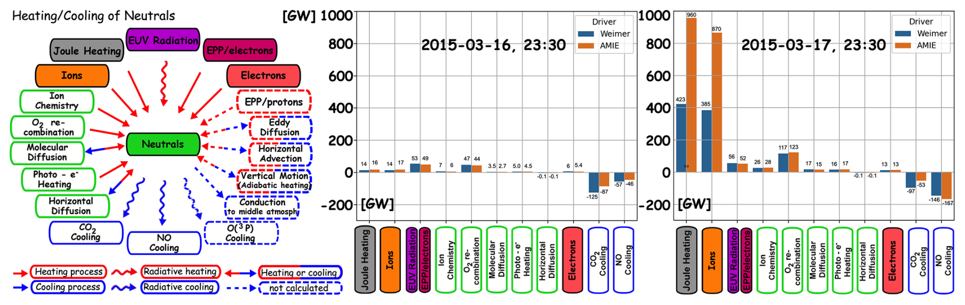
Figure 3 Left: Overview of the main energy sources and energy flow to and from the neutrals in the Lower Thermosphere–Ionosphere. Terms in solid arrows and boxes are estimated through TIE-GCM, whereas terms in dashed arrows and boxes are not calculated. Right (Middle): Quantification of the main energy terms at the peak of (one day before the peak of) St. Patrick's day storm. Two electric potential drivers are used, according to the Weimer 2005 and the AMIE models, as marked.

4.1 Energy Flow According to the Neutrals

The energy flow from and to the neutral species of the LTI is shown in the left panel of Fig. 3. As shown in this diagram, the neutrals are heated directly by EUV radiation, by Joule heating due to the differential velocity between the neutral winds and the ions under the effects of electric fields, by collisional interactions with the ions due to their differences in temperatures, by elastic collisions with electrons, by inelastic collisions with electrons, and by Energetic Precipitating Protons. The neutral species are cooled by heat conduction to the middle atmosphere, by horizontal and vertical heat advection, and by radiative cooling. The main radiative cooling elements in the LTI are CO₂ and NO. In principle, N₂ and O₂ also participate in IR radiation, however they are not included in TIE-GCM, and their radiative cooling effects are not included herein.

In the following, the energy sources and energy flow terms that are discussed in the left panel of Fig. 3 are calculated numerically based on TIE-GCM. In the middle and right panels of Fig. 3, two snapshots are plotted, corresponding to a quiet-time instance and to the peak of the storm. A movie of the evolution of these terms is included in Tourgaidis et al. (2025b). As discussed above, the peak of St. Patrick's day storm is defined by the time of minimum Dst and minimum SYM-H indices, which was on 17 March 2015, at 23:30. To illustrate the quiet-time energy sources and energy flow terms, a time instance one day before the peak of the storm is selected. Thus, the middle panel of Fig. 3 shows the quantification of the heating and cooling terms one day before the peak of St. Patrick's day storm, on 16 March 2015, at 23:30. This time is marked in Figure 1 with a blue dashed vertical line. At this time, small discrepancies can be seen in the two different estimates of Joule heating and the heating from the ions that are based on the different TIE-GCM runs with the two different external driving models, with the estimates that are based on the AMIE model showing larger amounts of heating compared to the Weimer model. As it is shown, the part of the Joule heating promptly deposited to the neutrals and the qΔT_in i.e. the heating of the neutrals due to collisions with the ions are almost equal, meaning that in quiet times half of the total Joule heating is promptly deposited to the neutrals and the other half goes directly to the ions and finally to the neutrals through ion-neutral collisions. Elastic and inelastic collisions with electrons are of little impact to the neutrals. The largest heating source during this time is the heating due to EUV and EPP heating followed by the heating due to the recombination of O₂. Radiative cooling by CO₂ is the largest cooling term, followed by the radiative cooling by NO. The least important heating terms are the heating due to the molecular diffusion, the horizontal diffusion and due to photoelectrons.

The right panel of Fig. 3 shows the quantification of the heating and cooling terms at the peak of St. Patrick's day storm, on 17 March 2015, at 23:30 UTC. This time is marked in Fig. 1 with a red dashed vertical line. In the right panel of Fig. 3, it is noted that Joule heating promptly deposited to the neutrals exceeds the heating deposited to the neutrals from the ions, which corresponds to the $q_{\mathrm{\Delta }{T}_{\text{in}}}$ term. Comparing the two different driving models, it is noted that the Weimer model gives lower estimates of Joule heating than the AMIE model. This, as discussed below, is attributed to the inclusion of smaller scales in the AMIE model, and also due to the fact that the AMIE model incorporates time-dependent observations and thus better reflects the state of the system. The heating due to EUV and EPP is only slightly elevated compared to the corresponding quiet time EUV and EPP heating. All the other heating terms, even though small compared to Joule heating and ion heating, are significantly increased with the exception of the heating due to horizontal diffusion. Regarding the cooling terms, it can be seen that CO₂ is a stronger cooling agent in the pre-storm time, whereas NO cooling is drastically increased post-storm, greatly exceeding CO₂ cooling. This has been reported in past studies, who have pointed out that during quiet times radiation in the IR is the dominant thermospheric cooling agent (see, e.g., Mlynczak et al., 2014), whereas cooling due to NO emission is greatly enhanced during storms, and is considered as a “natural thermostat” that contributes to the recovery of the thermosphere from the temperature increases due to Joule heating during solar geomagnetic storms, typically within 2–3 d (see, e.g., Mlynczak et al., 2003, 2005).

4.2 Energy Flow According to the Ions

The energy flow from and to the ion species of the LTI is shown schematically in Fig. 4. Thus, the ions are heated directly by Joule heating, due to the differential velocity between the neutral winds and ion drifts under the effects of electric fields. Ions also exchange energy with the electrons due to their differences in temperature, via electron-ion elastic collisions, that are dependent on the difference in temperatures between the electrons and the ions, according to Eq. (8). Finally, ions heat the neutral species via ion-neutral collisional interactions, due to their differences in temperatures, as discussed above and calculated via Eq. (7). A movie of the evolution of these terms is included in Tourgaidis et al. (2025b). In the middle panel of Fig. 4, corresponding to quiet-time conditions, we can see that, before the storm, Joule heating is the most significant heating source of the ions, and that the heating from the electrons is a small fraction (about 10 %) of the Joule heating. The total heating of the ions is transferred to the neutrals, which is considered a cooling term for the ions. In the right panel we can see that, at the peak of the storm, both the heating of the ions due to Joule heating and their cooling via heat transfer to the neutrals are largely increased.

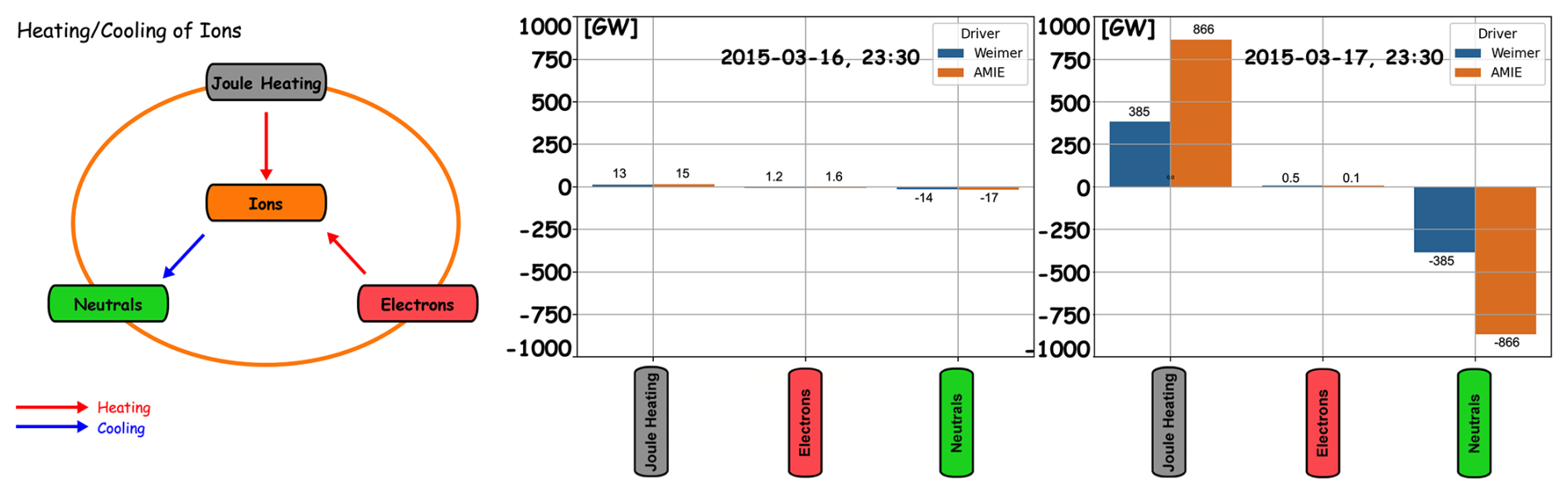
Figure 4 Left: Overview of the main energy sources and energy flow to and from the Ions in the Lower Thermosphere–Ionosphere. Terms in red arrows correspond to heating of the ions whereas terms in blue arrows correspond to cooling of the ions. Right (Middle): Quantification of the main energy terms at the peak of (one day before the peak of) St. Patrick's day storm. Two electric potential drivers are used, according to the models by Weimer 2005 and AMIE, as marked.

4.3 Energy Flow According to Electrons

The heating sources of electrons generally include solar EUV radiation, heating from electron precipitation, Joule heating, as well as heating from the deactivation of excited neutral and ion species and from the dissociative recombination of electrons with ions. On the other hand, electrons are cooled via electron-neutral elastic and inelastic collisions, as described in Eqs. (9) and (12), respectively (see Chap. 9.7 of Schunk and Nagy, 2009). Electrons are also cooled via collisions with the ions due to their temperature difference, as described in Eq. (8), as they are generally considered to be hotter than ions. Finally, electrons are also cooled by conduction. In TIE-GCM, only solar EUV radiation and energetic particle precipitation are considered as heating terms, while all other heating contributions are considered to be small and are neglected. As cooling terms, the energy transfer to the neutrals and ions is calculated. Furthermore, in TIE-GCM, a quasi-steady state is assumed for the electrons, and thus the thermal electric heat flux, horizontal gradients of electron temperature, T_e, and electron density, N_e, as well as adiabatic expansion and heat advection, are ignored. The heating and cooling sources of the electrons that are considered in the calculations herein are summarized schematically in the left panel of Fig. 5. The electron thermal conduction to lower altitudes, along their propagation parallel to the magnetic field, is not calculated herein; this is marked in a dashed blue box. The heating and cooling terms according to the electrons are presented quantitatively in the middle and right panels of Fig. 5, as above, whereas their time evolution is shown as a movie in Tourgaidis et al. (2025b). Both before and after the storm, there are very small differences between the heating and cooling rates between the Weimer 2005 and the AMIE model runs. Regarding the cooling rates, the differences of the cooling to the neutrals due to elastic collisions, and the cooling to the ions are very small. On the other hand the heat loss to the neutrals due to inelastic collisions become larger at the peak of the storm, following the pattern of the EUV/EPP heating. From the above, we can infer that at the peak of the storm the heating of the electrons is increased mostly due to enhanced EPP, and the cooling of the electrons is mainly controlled through the inelastic collisions with the neutrals.

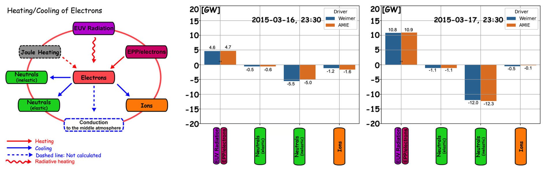
Figure 5 Left: Overview of the main energy sources and energy flow to and from the Electrons in the Lower Thermosphere–Ionosphere. Terms with red arrows correspond to heating of the electrons whereas terms with blue arrows correspond to cooling of the electrons. Right (Middle): Quantification of the main energy terms at the peak of (one day before the peak of) St. Patrick's day storm. Two electric potential drivers are used, according to the models by Weimer, and AMIE, as marked.

5 Discussion

Despite the comprehensive understanding of the basic framework that is presented in Fig. 2 and is demonstrated in the above calculations, there are significant gaps in the quantification of some of the key energy sources and processes, most notably Joule heating and the associated transfer of energy from the ions to the neutrals. This is primarily due to severe limitations in available data sets. It is noted, for example, that the entire available dataset of simultaneous ion, neutral and electron temperature measurements in the LTI at 100 to 200 km consists of only 60 h of observations (see, e.g., Fig. 11 of ESA-Daedalus-RfA, 2020), with the majority of measurements originating from the Atmosphere Explorer C and E satellites of the 1970s. Due to the lack of comprehensive measurements, the actual amount of Joule heating, the most important heating source in the LTI, varies greatly between estimation methodologies and input models. This has also been discussed and demonstrated in a study by Baloukidis et al. (2023), who compared Joule heating estimates from TIE-GCM and those derived from European Incoherent Scatter Scientific Association (EISCAT) radar measurements. That study found that TIE-GCM tends to overestimate Joule heating for low geomagnetic activity but underestimate them for high geomagnetic activity compared to EISCAT, and highlighted the need to account for small-scale effects in TIE-GCM. This has also been demonstrated by Tourgaidis et al. (2025a), who performed four different GCM simulations using TIE-GCM and GITM under two different electric potential models as external drivers, and compared the results against empirical model estimates. That study found that there are significant discrepancies between the GCMs, and even larger differences between GCMs and empirical models, that require new measurements and a revisit of the Joule heating estimates in the LTI.

Due to the lack of comprehensive co-located, co-temporal measurements, it is possible that even basic assumptions of the state of thermal equilibrium need to be revisited. For example, as recent re-analyses of the Atmosphere Explorer C, D and E datasets by Peterson et al. (2023) and Pirnaris and Sarris (2023) have shown, there are times when the temperatures of the neutrals, T_n, are higher than the temperatures of the ions, T_i, reversing the commonly accepted condition that T_i>T_n, which is enforced in current empirical models of the LTI, such as IRI-2020 (Bilitza et al., 2022) and NRLMSIS 2.0 (Emmert et al., 2021); this condition is also enforced in TIE-GCM v2.0. This leads to insufficient knowledge in understanding the effects of the external drivers to the overall energy budget and to the state variables of the LTI.

In comparing the various heating terms in Figs. 3–5, it can be seen that during the pre-storm time the heating due to EUV/EPP and the recombination of O₂ are the largest heating terms. At the peak of the storm, Joule heating and ion-neutral heating become the main heating sources by far, followed by the heating due to the recombination of O₂, whereas the heating due to the EUV/EPP is only slightly increased during the storm. Regarding the cooling of the neutrals, it can be seen that before the storm, the main cooling term is the CO₂ cooling, while at the peak of the storm the NO cooling becomes larger for both the AMIE and Weimer 2005 runs, although significant discepancies can be seen in their estimates.

With respect to the differences in the estimates of Joule heating between the Weimer 2005 and the AMIE models, it is noted that one crucial difference between the two model runs is the spatial scales that can be resolved by each. The Weimer-2005 empirical model has a resolution of ∼ 2–3° in magnetic latitude and ∼ 1h in MLT. On the other hand, the AMIE assimilative model is in general finer than empirical models, but is highly dependent on available data density. Typically, the AMIE model can achieve a resolution of ∼ 1–2° in magnetic latitude and ∼ 15–30 min in MLT. On the other hand, the grid resolution of TIE-GCM is 2.5° × 2.5° in latitude and longitude. Thus, due to its coarse spatial resolution, TIE-GCM cannot resolve small-scale (sub-grid) electric field variability. In reality though, the small-scale electric field variability can greatly enhance Joule heating due to its quadratic dependence on the electric field (Q_J=Σ_PE²); thus an underestimation of Joule heating is expected in the model, if sub-grid variability is not well represented. To partially compensate this, TIE-GCM employs an empirical Joule heating enhancement factor, termed Joulefac, which scales the modeled heating to account for unresolved small-scale structures. This approach provides a climatologically reasonable estimate of total heating but may underestimate localized responses during disturbed conditions. Moreover, the use of higher resolution electric fields from assimilative techniques instead of empirical models, compensates part of the small-scale variability but nevertheless, residual underestimation persists (i.e. scales below 1°). As discussed in Baloukidis et al. (2023), using a Joulefac parameter that is dependent on the solar wind parameters is required, but this relies on critically missing measurements in the LTI, where Joule heating maximizes.

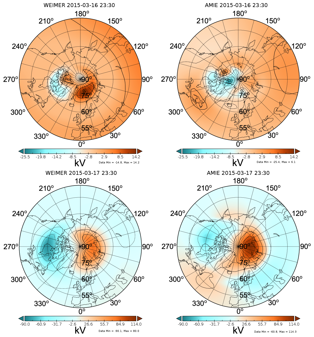
Figure 6 Electric potential maps: Upper-left: Weimer at baseline, Upper-right: AMIE at baseline, Lower-left: Weimer at peak, Lower-right: AMIE at peak.

To investigate the effect of the average electric field on the observed discrepancies in the modeled Joule heating, in Fig. 6 we plot the high-latitude electric potential for the two models and for the two time-steps used in this study. In the left-hand side of this figure the Weimer-2005 model results are given, whereas in the right-hand side figure the results of the AMIE model are given. As it can be seen from these panels, the Weimer-2005 model gives higher potential at the pre-storm baseline timestep, while the AMIE model gives higher potential at the peak of the storm. At the baseline timestep, the potential patterns of the two models are spatially different, while at the peak of the storm both models capture the two-cell structures quite similarly.

Another key missing aspect of Joule heating involves the characterization of its altitudinal distribution. Whereas ground-based measurements can provide the altitude profiles of Joule heating, they lack the required resolution, and also do not provide all measurements that are required in the estimation of Joule heating. As demonstrated by Vogt et al. (2023), a twin-spacecraft mission with altitudinal separation and with comprehensive instrumentation that performs measurements near the altitudes of interest would be able to provide the altitude profiles down to a couple of atmospheric scale heights under the spacecraft. This is essential for an LTI mission and would enable measurements with sufficient statistical significance, so as to derive the climatological characterization of Joule heating as a function of altitude, while also resolving the open question of the significance of Joule heating at small scales.

With respect to the differences in the heat exchange rates between ions and neutrals between the two model runs, it is noted that these are proportional to the Joule heating rate estimates, as shown in Figs. 3 and 4. This is because the heat exchange rates between ions and neutrals via collisional interactions will depend on the corresponding temperatures, T_i and T_n, as shown in Eq. (7). Since different Joule heating rates will result in different temperature increases of the ions, a higher Joule heating rate is indeed expected to result in higher ion-neutral heat exchange, as it is observed herein.

In Fig. 3, it can be seen that the cooling terms from the main radiative cooling species, NO and CO₂, are also significantly different for the two runs with the different drivers, both before the storm and during the peak of the storm, due to the different external drivers and the resulting different neutral temperatures of the LTI region.

It is noted that heat advection and heat conduction are also calculated in TIE-GCM and are a part of the energy budget of the neutrals and plasmas. The heat conduction term depends on gradients in temperature, whereas the heat advection will depend on gradient in the velocity. These terms are calculated at every step in TIE-GCM, but are not included in the presented analysis.

6 Summary and Conclusions

The storage, transport and transformation of energy in the Lower Thermosphere–Ionosphere (LTI) was studied via model runs using NCAR's TIE-GCM in order to estimate energy sources and sinks, energy transfer rates and the energy partitioning between the different species. The model runs were performed for the 2015 St. Patrick's day geomagnetic super-storm, for the period 15–21 March. To explore the variability in the quantification of the energy budget and energy flow, we performed estimates from two different simulations of TIE-GCM, using two different high latitude potential models as external drivers: one empirical model, Weimer 2005, and one assimilative model, AMIE. The resulting energy budget and the corresponding partitioning of energy between species were inter-compared between the two runs, before and after the storm. These two runs allow to explore the range of variability of various heating and cooling terms under the effect of the largely unknown high-latitude electric potential. We then quantified the variability of the main energy flow estimates from three different perspectives: that of the neutrals, of the ions and of the electrons, as different heating and cooling mechanisms are associated with each species. It is noted that, whereas in most studies the state of the LTI is presented from the viewpoint of the neutrals, herein a view of the main energy transfer terms is presented separately according to each species.

It was found that the largest differences in the energy flow for the different processes is observed primarily in the Joule heating rates, and in the associated heating from the ions to the neutrals. Specifically, it was found that the AMIE model run gives more than twice as large Joule heating and ion-to-neutral heating than the Weimer 2005 model. These discrepancies are attributed to the average electric field that is estimated by each of the model drivers, as higher fields will give higher Joule heating. The discrepancies are also due to the different temporal variability in the electric field and also due to the differences in the small spatial scales of the electric field that can be resolved by each of the models, as higher spatial and temporal variability will result in higher Joule heating. This sub-grid variability of the electric fields is a key unknown factor in LTI electrodynamics and energetics, and has significant implications for the quantification and prediction of the effects of energy inputs such as Joule heating for density enhancements in the LTI and the resulting drag effects on Low Earth Orbit satellites. The recently released TIEGCM 3.0 (High Altitude Observatory, 2025) offers higher spatial resolution compared to TIEGCM 2.0 that was used in this study, and subsequent investigations are needed to investigate the effects of smaller-scale sub-grid variability on the resulting Joule heating.

Together with the above issues related to spatial resolution of the models, the discrepancies are also related to the fundamental differences of the forcing models: whereas the Weimer (2005) model represents a statistical, climatological average response to given solar wind and IMF conditions, the AMIE model incorporates time-dependent observations and thus better reflects the actual, event-specific electrodynamic state of the system. During the storm maximum, when the magnetosphere–ionosphere system departs significantly from an average behavior, deviations from climatological patterns become substantial. Under such highly disturbed conditions, the use of boundary conditions that closely represent the instantaneous electrodynamics becomes particularly critical. The enhanced Joule heating in the AMIE-driven simulation therefore likely reflects a more realistic representation of the storm-time energy input.

The quantification of the various energy terms, their variability, and the discrepancies between models, highlights the need for the accurate quantification of Joule heating, as the single most important term with the highest magnitude and highest variability, both during the evolution of the storm-time event that was simulated, but also when different model runs are inter-compared. This has significant implications for our knowledge and understanding of the storm-time response of the LTI to the external forcing. Through the model runs it is concluded that obtaining new, systematic measurements of all required parameters for the calculation of Joule heating is required to improve our understanding of the energy balance and energy transfer processes. Obtaining co-located, co-temporal measurements within this region requires placing state-of-the-art instruments on an in situ platform that samples this region along track, providing statistically significant measurements (e.g., Sarris et al., 2023a). Such mission concepts are actively pursued at ESA and NASA (e.g., Sarris et al., 2020; Pfaff et al., 2022; ESA/NASA-ENLoTIS-Report, 2024). The measurements gathered in this manner will enable estimating the actual Joule heating into the LTI and will reveal how collisions between neutral and charged species affect the energetics of the LTI, providing a critically missing link in the energy budget of the LTI.