What is the neutral wind in height-integrated ionospheric electrodynamics?

In many studies of the electrodynamics of the coupled ionosphere-thermosphere (IT) system at high latitudes, the ionosphere is represented as a two-dimensional spherical shell and the height-integrated ionospheric Ohm's law is used to understand IT electrodynamic coupling. Thermospheric winds play a central role in IT electrodynamics, but they are generally ignored in existing empirical models and assimilative methods. While the primary issue is a lack of comprehensive wind measurements, there is also a gap in the literature on how to represent the thermospheric winds – which often exhibit strong variations with altitude – in a height-integrated description of high-latitude IT electrodynamics, and what the associated sources of error might be. Here we highlight that there is in general no single suitable definition of the neutral wind term in high-latitude, height-integrated IT electrodynamics. Instead, two neutral wind terms weighted by Hall and Pedersen conductivities appear in the height-integrated Ohm's law. Using altitude profiles of neutral winds and ionospheric conductivities respectively derived from sounding rocket chemical release experiments near Poker Flat, Alaska, and Poker Flat Incoherent Scatter Radar (PFISR) measurements, we find magnitude differences of order 10–100 m s⁻¹ between the two neutral wind terms. The difference in magnitude increases with increasing geomagnetic activity. We show that a commonly used expression for Joule heating in terms of height-integrated quantities is a lower bound of the actual height-integrated Joule heating. We demonstrate how during geomagnetically quiet periods both the magnitude and direction of the neutral wind may influence total Joule heating, while during active periods the neutral wind influences total Joule heating primarily via its orientation relative to the plasma convection. We also find that measurements of the thermospheric wind at altitudes of ∼100–120 km are a more accurate estimate of the thermospheric wind terms in expressions of height-integrated, high-latitude electrodynamics than simply assuming the neutral winds are zero in Earth's corotating frame of reference. This points to the possible utility of, for example, Fabry–Perot interferometers that measure 557.7-nm (green-line) emissions around this altitude range.

1 Introduction

Earth's overlapping ionosphere-thermosphere (IT) region is the site of mechanical and electrodynamic coupling between the neutral atmosphere and plasmas of both terrestrial (magnetospheric and ionospheric) and extraterrestrial (solar wind) origin. Much of the electrodynamics within this region can be described in terms of a three-fluid model consisting of neutral, ion, and electron fluids in the presence of a strong background magnetic field (see Sect. 9.5 in Parker, 2007).

A common point of reference for a vast number of experimental investigations of high-latitude IT electrodynamics is the component of the ionospheric Ohm's law that is perpendicular to the main magnetic field, assuming steady-state stress balance between Lorentz and collisional drag forces and neglecting all other forces in the ion momentum equation (Sect. 5 in Chapman, 1956; Sect. 3.2.1 in Vasyliunas, 2012):

$$\begin{array}{}\text{(1)}& {\displaystyle }{\displaystyle }{\mathit{j}}_{⟂}={\mathit{\sigma }}_{\mathrm{P}}\left({\mathit{E}}_{⟂}+\mathit{u}\times \mathit{B}\right)+{\mathit{\sigma }}_{\mathrm{H}}\mathit{b}\times \left({\mathit{E}}_{⟂}+\mathit{u}\times \mathit{B}\right),\end{array}$$

with j_⟂ the perpendicular current density, σ_P and σ_H the Pedersen and Hall conductivities, and E_⟂, B, and u the perpendicular ionospheric electric field, the total (background plus perturbation) magnetic field, and the thermospheric wind. The unit vector b points in the direction of B. The corresponding Joule heating (heating rate per volume) is given by

$$\begin{array}{}\text{(2)}& {\displaystyle }{\displaystyle }{w}_J={\mathit{j}}_{⟂}\cdot \left({\mathit{E}}_{⟂}+\mathit{u}\times \mathit{B}\right)={\mathit{\sigma }}_{\mathrm{P}}|\left({\mathit{E}}_{⟂}+\mathit{u}\times \mathit{B}\right){|}^{\mathrm{2}}.\end{array}$$

Both j_⟂ and w_J are independent of reference frame in (magnetic) Galilean relativity (Mannucci et al., 2022) by virtue of the fact that they are defined in terms of the sum of the electric field and the “neutral wind dynamo” u×B.

Some notable experimental investigations of Eqs. (1) and (2) include that of Thayer (1998) and those based on the Joule II suborbital sounding rocket campaign (Sangalli et al., 2009; Burchill et al., 2012), while others have focused on experiment-model comparisons, modeling, or theoretical aspects (e.g. Baloukidis et al., 2023; Song et al., 2005; Strangeway, 2012). Thayer (1998) used incoherent scatter radar measurements at a temporal resolution of ∼17 min to present the first examination of how the neutral wind u modifies height profiles of Joule heating. The Joule II-based study of Sangalli et al. (2009) used in situ measurements of electric field, bulk ion drift, neutral wind, and electron density in the vicinity of a relatively quiescent auroral breakup in northern Alaska to estimate the errors in E-region ion-neutral momentum transfer collision frequency and Joule heating altitude profiles that would arise if the neutral winds were assumed to be zero. In their separate analysis of these and additional rocket and ground-based observations from the same campaign, Burchill et al. (2012) found evidence for horizontal or vertical structuring in ion-neutral collision frequencies on scales of 1–10 km.

Comprehensive measurements of altitude profiles such as those presented by Sangalli et al. (2009) and Burchill et al. (2012) are rare. Much more frequently one encounters a height-integrated form of the ionospheric Ohm's law:

$$\begin{array}{}\text{(3)}& {\displaystyle }{\displaystyle }{\mathit{J}}_{⟂}={\mathrm{\Sigma }}_{\mathrm{P}}\left({\mathit{E}}_{⟂}+\mathit{U}\times \mathit{B}\right)+{\mathrm{\Sigma }}_{\mathrm{H}}\mathit{b}\times \left({\mathit{E}}_{⟂}+\mathit{U}\times \mathit{B}\right),\end{array}$$

where Σ_P and Σ_H are the Pedersen and Hall conductances (conductivities integrated over altitude, explicitly ${\mathrm{\Sigma }}_c=\int {\mathit{\sigma }}_c\mathrm{d}h$ with c either H or P). This form is obtained by integrating Eq. (3) over altitude assuming that B is radial, that B and E_⟂ are independent of altitude over ionospheric E- and F-region altitudes (∼100–250 km), and that U is a height-averaged neutral wind, or a representative or effective neutral wind. Most often the wind is “neglected”, which is generally equivalent to assuming it is zero in Earth's rotating frame of reference (e.g. Amm, 1995; Amm et al., 2008; Vanhamäki and Juusola, 2018; Matsuo, 2020; Weimer and Edwards, 2021). (Appendix A provides a brief summary of the implications of assuming the E-field is constant with altitude.) One also encounters an expression for the height-integrated Joule heating rate,

$$\begin{array}{ll}{\displaystyle }{W}_J& {\displaystyle }=\int w_J\mathrm{d}h={\mathit{J}}_{⟂}\cdot \left({\mathit{E}}_{⟂}+\mathit{U}\times \mathit{B}\right)\\ \text{(4)}& {\displaystyle }& {\displaystyle }={\mathrm{\Sigma }}_{\mathrm{P}}{\left({\mathit{E}}_{⟂}+\mathit{U}\times \mathit{B}\right)}^{\mathrm{2}},\end{array}$$

that is also defined in terms of a typically unspecified or unused effective neutral wind U. Last, one encounters estimates of ionospheric conductances via the expressions likewise defined in terms of U,

$$\begin{array}{}\text{(5)}& {\displaystyle }& {\displaystyle }{\mathrm{\Sigma }}_{\mathrm{H}}=-\widehat{\mathit{b}}\cdot \left[{\mathit{J}}_{⟂}\times \left({\mathit{E}}_{⟂}+\mathit{U}\times \mathit{B}\right)\right]/|{\mathit{E}}_{⟂}+\mathit{U}\times \mathit{B}{|}^{\mathrm{2}};\text{(6)}& {\displaystyle }& {\displaystyle }{\mathrm{\Sigma }}_{\mathrm{P}}={\mathit{J}}_{⟂}\cdot \left({\mathit{E}}_{⟂}+\mathit{U}\times \mathit{B}\right)/|{\mathit{E}}_{⟂}+\mathit{U}\times \mathit{B}{|}^{\mathrm{2}}.\end{array}$$

The approach represented by Eq. (4) for estimating height-integrated Joule heating based on height-integrated quantities dates at least back to the work of Cole (1975) and continues to be used widely (see Thayer, 1998, and references therein). The study of Billett et al. (2018) stands out as the only observational study of global distributions of ionospheric Joule heating that has included information, via an empirical model, about an effective wind pattern. On the other hand, the approach represented by Eqs. (5) and (6) for estimating conductances based on height-integrated quantities originates with Amm (2001). This approach has been used by a number of studies over the past two decades, and has elsewhere been referred to as the “electrodynamic method” (e.g. Green et al., 2007; Weimer and Edwards, 2021; Hatch et al., 2024). To our knowledge, all published studies in which conductance distributions have been estimated experimentally via Eqs. (5) and (6) have assumed U=0 (Amm, 1995; Amm et al., 2015; Weimer and Edwards, 2021; Hatch et al., 2024).

The height-integrated approach to ionospheric electrodynamics represented by Eqs. (3)–(6) is heavily simplified: Earth's magnetic field lines are not radial, ionospheric electric fields do not necessarily map along field lines (Farley, 1959), and the horizontal components of the neutral wind exhibit the nearly permanent presence of vertical shears over altitudes of 80–140 km (Heppner and Miller, 1982; Larsen, 2002; Sangalli et al., 2009). More advanced treatments of ionospheric electrodynamics that account for such complications, such as that presented by Richmond (1995), nevertheless remain unused in a large number of experimental studies and data assimilation techniques (e.g. Richmond and Kamide, 1988; Matsuo, 2020; Laundal et al., 2022, 2025a), primarily for lack of a body of robust 3D measurements of the IT system needed to make use of them (Palmroth et al., 2021). For similar reasons, in the majority of existing global MHD models the coupling between the magnetosphere and the IT system is founded on what Mannucci et al. (2022) term a “key magnetosphere-ionosphere coupling equation” derived from current continuity (their Eq. 11; see also Merkin and Lyon, 2010; Mukhopadhyay et al., 2021, and references therein) in which the neutral wind is assumed to be zero or constant with altitude.

In this study, we explore some of the implications of the commonly employed assumption that the neutral wind is independent of altitude that is necessary to arrive at Eqs. (3)–(6) as well as the current continuity equation used in magnetosphere-ionosphere coupling. In Sect. 2 we summarize central quantities and equations in a height-integrated description of IT electrodynamics when the neutral wind is not assumed to be independent of altitude. In Sect. 3 we present three basic questions that are raised by this alternative formalism, and answer them using neutral wind profiles derived from rocket-borne trimethylaluminum (TMA) chemical release experiments launched from the Poker Flat Research Range (PFRR) between 2007–2018 together with conductivity profiles calculated from measurements made by the Poker Flat Incoherent Scatter Radar (PFISR). In Sect. 4 we summarize our findings, and discuss how they can be used to understand the role of the neutral winds in 2D descriptions of IT electrodynamics.

2 Defining the neutral wind in height-integrated IT electrodynamics

If one assumes that u does vary with height, integration of Ohm's law (Eq. 1) over ionospheric altitudes yields

$$\begin{array}{}\text{(7)}& {\displaystyle }{\displaystyle }{\mathit{J}}_{⟂}={\mathrm{\Sigma }}_{\mathrm{P}}{\mathit{F}}_{\mathrm{P}}+{\mathrm{\Sigma }}_{\mathrm{H}}\widehat{\mathit{b}}\times {\mathit{F}}_{\mathrm{H}}\end{array}$$

where

$$\begin{array}{}\text{(8)}& {\displaystyle }& {\displaystyle }{\mathit{F}}_c={\mathit{E}}_{⟂}+{\mathit{U}}_c\times \mathit{B};\text{(9)}& {\displaystyle }& {\displaystyle }{\mathit{U}}_c={\displaystyle \frac{\mathrm{1}}{{\mathrm{\Sigma }}_c}}\int {\mathit{\sigma }}_c\mathit{u}\mathrm{d}h;\end{array}$$

and c is either H or P. The integration is performed over all ionospheric altitudes. We refer to the conductivity-weighted neutral wind terms U_H and U_P as the Hall-weighted or Pedersen-weighted neutral winds. The latter has been termed the “effective neutral wind” by Lu et al. (1995) and plays a role in estimates of height-integrated Joule heating and the Pedersen conductance, which we discuss later in this section. The distinction between the Hall-weighted and Pedersen-weighted neutral winds disappears when the two conductivity profiles differ by no more than a constant factor, or when the neutral wind u does not vary with altitude. As noted in the Introduction, these idealized conditions are rarely manifest in measured altitude profiles of the conductivities and neutral winds (e.g. Larsen, 2002).

Integrating the right-hand side of the expression for Joule heating density (Eq. 2), we obtain the height-integrated Joule heating rate

$$\begin{array}{ll}{\displaystyle }& {\displaystyle }{W}_J=\int w_J\mathrm{d}h=\int {\mathit{\sigma }}_{\mathrm{P}}|\left({\mathit{E}}_{⟂}+\mathit{u}\times \mathit{B}\right){|}^{\mathrm{2}}\mathrm{d}h\\ \text{(10)}& {\displaystyle }& {\displaystyle }={\mathrm{\Sigma }}_{\mathrm{P}}\left[E_{⟂}^{\mathrm{2}}+\mathrm{2}{\mathit{E}}_{⟂}\cdot \left({\mathit{U}}_{\mathrm{P}}\times \mathit{B}\right)\right]+\int {\mathit{\sigma }}_{\mathrm{P}}|\mathit{u}\times \mathit{B}{|}^{\mathrm{2}}\mathrm{d}h.\end{array}$$

Because of the integral in the last term involving $|\mathit{u}\times \mathit{B}{|}^{\mathrm{2}}$, this expression cannot directly be brought into the more familiar form ${\mathrm{\Sigma }}_{\mathrm{P}}{\left({\mathit{E}}_{⟂}+\mathit{U}\times \mathit{B}\right)}^{\mathrm{2}}$ for some appropriately chosen U (cf. Eq. 4). However, one may show explicitly via the Cauchy–Bunyakovsky–Schwarz inequality (see Appendix B) that $\int {\mathit{\sigma }}_{\mathrm{P}}\Vert \mathit{u}\times \mathit{B}{\Vert }^{\mathrm{2}}\mathrm{d}h\ge {\mathrm{\Sigma }}_{\mathrm{P}}{\left({\mathit{U}}_{\mathrm{P}}\times \mathit{B}\right)}^{\mathrm{2}}$. Then the following inequalities hold:

$$\begin{array}{ll}{\displaystyle }& {\displaystyle }{W}_J\ge {\mathrm{\Sigma }}_{\mathrm{P}}{\left({\mathit{E}}_{⟂}+{\mathit{U}}_{\mathrm{P}}\times \mathit{B}\right)}^{\mathrm{2}}={\mathrm{\Sigma }}_{\mathrm{P}}{F}_{\mathrm{P}}^{\mathrm{2}};\\ \text{(11)}& {\displaystyle }& {\displaystyle }{\mathrm{\Sigma }}_{\mathrm{P}}\le W_J/F_{\mathrm{P}}^{\mathrm{2}}.\end{array}$$

Thus when the “effective” neutral wind U is specified to be the Pedersen-weighted neutral wind U_P in Eqs. (4) and (6), these equations are in fact lower and upper bounds, respectively, on the true height-integrated Joule heating and Pedersen conductance. When the neutral wind does not vary with altitude we have ${\mathit{U}}_{\mathrm{P}}={\mathit{U}}_{\mathrm{H}}=\mathit{U}$ in Inequality (11), such that the height-integrated Joule heating $W_J={\mathrm{\Sigma }}_{\mathrm{P}}(\mathit{E}+\mathit{U}\times \mathit{B}{)}^{\mathrm{2}}$ and the Pedersen conductance ${\mathrm{\Sigma }}_{\mathrm{P}}=W_J/(\mathit{E}+\mathit{U}\times \mathit{B}{)}^{\mathrm{2}}$ as given by Eqs. (4) and (6).

From the foregoing we see that for estimation of height-integrated Joule heating, the Pedersen-weighted neutral wind U_P constitutes the most natural definition of the “effective” neutral wind, as indirectly suggested by Lu et al. (1995).

3 Experimental investigation of Hall- and Pedersen-weighted neutral winds

Equations (7)–(9) illustrate that there is in general not one, but two, neutral wind terms in height-integrated treatments of IT electrodynamics. The neutral wind appears as two separate terms weighted separately by the Hall and Pedersen conductivity profiles, here defined by Eq. (9) and respectively denoted by U_H and U_P. This situation raises the following questions:

1. How large is the observed difference between U_H and U_P? (Sect. 3.2)

2. How much better are various rule-of-thumb approximations for the neutral wind (e.g. the suggestion from Lu et al., 1995, that the “winds at 160 km” are representative of the ”effective neutral wind”) than simply assuming ${\mathit{U}}_{\mathrm{H}}={\mathit{U}}_{\mathrm{P}}=\mathit{u}=\mathrm{0}$? (Sect. 3.3)

3. How much does the lower-bound approximation Σ_P(U_P×B)² underestimate the true contribution of the purely wind-dependent term $\int {\mathit{\sigma }}_{\mathrm{P}}\Vert \mathit{u}\times \mathit{B}{\Vert }^{\mathrm{2}}\mathrm{d}h$ in the expression for height-integrated Joule heating given by Eq. (10)? (Sect. 3.4)

To answer these questions we use horizontal neutral wind profiles derived from TMA chemical release experiments carried by sounding rockets during five campaigns launched from PFRR (Mesquita, 2021, and references therein), as well as vertical conductivity profiles derived from PFISR measurements and empirical models of ionospheric and atmospheric composition, atmospheric temperature, and Earth's magnetic field.

3.1 Measurements and models

Figure 1 shows a summary of the 15 wind profiles used in this study, with the zonal and meridional components displayed respectively in the left and center columns, and the horizontal magnitudes in the right column. The vertical component is not estimated and is ignored throughout this study. The text label at right shows the date, campaign name, and K_p value for each group of wind profiles. The chronological ordering of the rows of Fig. 1 coincidentally also orders the wind profiles by K_p, aside from the last row (Super Soaker campaign) for which K_p was lowest (K_p=0.3). The magnitudes of the wind profiles show a clear tendency to increase with increasing K_p.

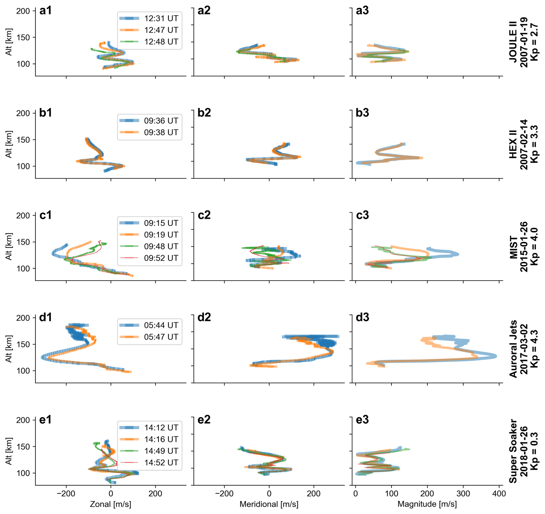
Figure 1 Summary of neutral wind profiles used in this study, given in the same order as the rocket campaigns in Table 1. The zonal and meridional components are shown in the left and center columns, with the magnitude profiles shown in the right column. The campaign name and degree of geomagnetic activity are indicated in the caption at far right in each row.

Table 1 summarizes some details of each rocket, including the time of each measurement (center time of images used for triangulation of chemical release experiments) and the availability of PFISR measurements.

Burchill et al. (2012)Sangalli et al. (2009)Scott (2009)Larsen et al. (2022)Akbari et al. (2022)Mesquita et al. (2020)

Table 1 Rockets from which neutral wind measurements are used in this study.

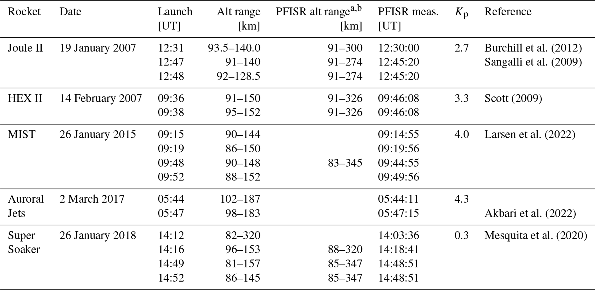
^a We exclude PFISR measurements for which ${\mathit{\sigma }}_{n_e}/n_e\ge \mathrm{1}$. (n_e: plasma density. ${\mathit{\sigma }}_{n_e}$: plasma density uncertainty).
^b Valid PFISR measurements are available over 87–345 km unless otherwise noted. Vertical (elevation = 90°) beam measurements are used.

For each wind profile shown in Fig. 1 we calculate corresponding U_H and U_P vectors via Eq. (9). This calculation requires conductivity profiles, which we calculate using PFISR measurements, the NRLMSIS^® 2.0 empirical atmospheric model (Emmert et al., 2020), and the International Reference Ionosphere (IRI) 2016 model (Bilitza et al., 2017), following the methodology of Ieda (2020). The steps of this process are summarized and illustrated in Appendix C and Fig. C1.

3.2 Statistics of U_H and U_P

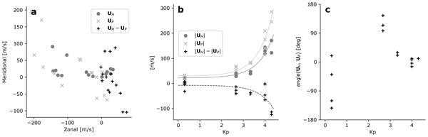
After performing the procedure described in the previous subsection for all 15 neutral wind profiles, we obtain the estimates of U_H and U_P as well as their difference (U_H−U_P) shown in Fig. 2a. For these neutral wind profiles the zonal component of U_H and U_P tend to be negative (westward), while the meridional components tend to be positive (northward). The magnitudes of U_H and U_P are of order 10–100 m s⁻¹. Given the magnitude of the geomagnetic field at PFRR (∼54 000 nT at 110 km altitude), these magnitudes correspond to electric field equivalents of ∼0.5–5 mV m⁻¹.

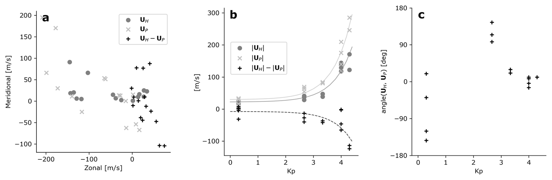
Figure 2 (a) Statistics of U_H, U_P, and U_H−U_P. (b) The magnitude of U_H and U_P, and the difference in magnitudes, vs. K_p. The solid lines are nonlinear fits of the form $a\exp (K_{\mathrm{p}}/b)+c$ to $\left|{\mathit{U}}_{\mathrm{H}}\right|$ and $\left|{\mathit{U}}_{\mathrm{P}}\right|$, and the dashed line their difference. (c) The angle measured from the direction of U_H to the direction U_P vs. K_p. These plots answer Question 1 posed at the beginning of Sect. 3 (“How large is the observed difference between U_H and U_P?”).

Figure 2b plots the magnitudes of U_H and U_P and shows that they increase approximately exponentially with increasing K_p. The difference $\left|{\mathit{U}}_{\mathrm{H}}\right|-\left|{\mathit{U}}_{\mathrm{P}}\right|$ (black crosses) is almost everywhere negative; the only two instances in which $\left|{\mathit{U}}_{\mathrm{H}}\right|>\left|{\mathit{U}}_{\mathrm{P}}\right|$ are found for K_p=0.3. The difference is increasingly negative for increasing K_p.

The solid lines in Fig. 2 demonstrate that an exponential function of the form $a\exp (K_{\mathrm{p}}/b)+c$ suitably describes the magnitudes of U_H and U_P. The dashed line displays the difference between these fit functions and follows the overall trend of $\left|{\mathit{U}}_{\mathrm{H}}\right|-\left|{\mathit{U}}_{\mathrm{P}}\right|$. Fit parameters for $\left|{\mathit{U}}_{\mathrm{H}}\right|$ and $\left|{\mathit{U}}_{\mathrm{P}}\right|$ are derived by performing a nonlinear regression that minimizes the residuals for all three sets of points shown in Fig. 2 simultaneously, subject to Huber loss (Huber, 1973), to provide a robust estimate of the best-fit parameters. The fits are performed using the least_squares function of SciPy (Virtanen et al., 2020). We obtain similar results (not shown) with a standard linear loss function and when each of the sets of points are fit separately.

Figure 2c displays the angle between U_H and U_P measured from the direction of U_H to the direction of U_P. This is calculated as

$${\displaystyle }\text{angle}({\mathit{U}}_{\mathrm{H}},{\mathit{U}}_{\mathrm{P}})=\text{atan2}\left(U_{\mathrm{H},y},U_{\mathrm{H},x}\right)-\text{atan2}\left(U_{\mathrm{P},y},U_{\mathrm{P},x}\right),$$

where x and y refer respectively to the zonal and meridional wind components. The angle appears to tend toward zero for increasing K_p, indicating that U_H and U_P tend to become more aligned with increasing geomagnetic activity.

3.3 Proxies for the Hall- and Pedersen-weighted neutral winds

Here we address Question 2 posed at the beginning of this section: How much better are various rule-of-thumb approximations for the neutral wind than simply assuming ${\mathit{U}}_{\mathrm{H}}={\mathit{U}}_{\mathrm{P}}=\mathit{u}=\mathrm{0}$? To answer this question, Fig. 3a shows the error distribution $\text{Error}\left({\mathit{U}}_{\mathrm{P}}={\mathit{u}}_{\text{proxy}}\right)=|{\mathit{U}}_{\mathrm{P}}-{\mathit{u}}_{\text{proxy}}|$ associated with the assumption U_P=u_proxy, where u_proxy is taken to be one of 0, u₁₆₀, ${\mathit{u}}_{{\mathit{\sigma }}_{\mathrm{P}}\text{peak}}$, or ${\mathit{u}}_{{\mathit{\sigma }}_{\mathrm{H}}\text{peak}}$. These are respectively the zero vector, the neutral wind at 160 km altitude, the neutral wind at the altitude where the Pedersen conductivity profile peaks, and the neutral wind at the altitude where the Hall conductivity profile peaks. Each distribution is presented as a vertical box-and-whisker plot, where each box indicates (from top to bottom) the upper quartile Q3, the median, and lower quartile Q1. The horizontal lines above and below are respectively given by the largest value not exceeding Q3+1.5IQR and the smallest value not below Q1−1.5IQR, where $\text{IQR}=Q\mathrm{3}-Q\mathrm{1}$ is the interquartile range. (The range Q1−1.5IQR to Q3+1.5IQR is a common rule of thumb for identifying statistical outliers; see, e.g. Dekking et al., 2005.) In Fig. 3a these lines simply indicate the minimum and maximum of each distribution, since no values are outside these thresholds.

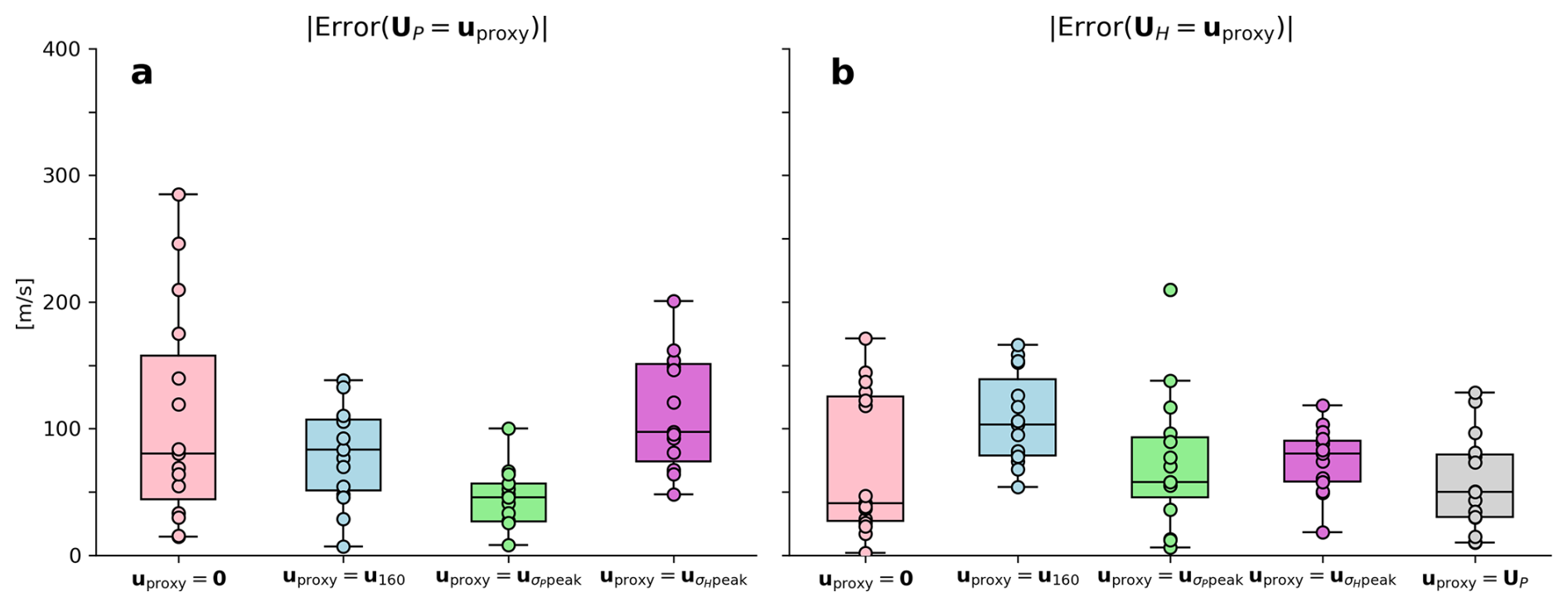
Figure 3 (a) For 15 neutral wind profiles, box-and-whisker plots of the magnitude of the Pedersen-weighted neutral wind (U_P, pink), the magnitude of the differences between U_P and the neutral wind at 160 km altitude (u₁₆₀, blue), the magnitude of the difference between U_P and the neutral wind at the height at which the Pedersen conductance maximizes (${\mathit{u}}_{{\mathit{\sigma }}_{\mathrm{P}}\text{peak}}$, green), and the magnitude of the difference between U_P and the neutral wind at the height at which the Hall conductance maximizes (${\mathit{u}}_{{\mathit{\sigma }}_{\mathrm{H}}\text{peak}}$, violet). The first and second represent the error associated with assuming U_P=0 m s⁻¹ and U_P=u₁₆₀; the latter two represent the error associated with assuming U_P is one of the two proxies. The horizontal lines above and below each box-and-whisker plot are the minimum and maximum except in panel (b) for ${\mathit{u}}_{\text{proxy}}={\mathit{u}}_{{\mathit{\sigma }}_{\mathrm{P}}\text{peak}}$, shown in green, where one value is an outlier (see main text). (b) Same layout as panel (a), but for the Hall-weighted neutral wind U_H and with an additional box-and-whisker plot (gray at far right) to assess U_H=U_P. The point of this figure is to answer Question 2 posed at the beginning of Sect. 3 by assessing whether any proxy for the Hall- and Pedersen-weighted neutral winds statistically incurs less error than simply assuming that they are zero.

In analogy with Fig. 3a, Fig. 3b shows the error associated with assuming U_H=u_proxy. One value in the distribution of errors for ${\mathit{u}}_{\text{proxy}}={\mathit{u}}_{{\mathit{\sigma }}_{\mathrm{P}}\text{peak}}$ (shown in green) is identified as an outlier.

Figure 3a demonstrates that for the 15 neutral wind profiles examined in this study, assuming ${\mathit{U}}_{\mathrm{P}}={\mathit{u}}_{{\mathit{\sigma }}_{\mathrm{P}}\text{peak}}$ (green) statistically incurs less error than assuming U_P=0 (pink), U_P=u₁₆₀ (blue), or ${\mathit{U}}_{\mathrm{P}}={\mathit{u}}_{{\mathit{\sigma }}_{\mathrm{H}}\text{peak}}$ (purple). For U_H, Fig. 3b shows that assuming U_H=0 (pink) incurs the lowest median error of any proxy, although the median error and overall range of errors is also similar for all of the remaining proxies besides u₁₆₀.

Lu et al. (1995) found via simulation that the “effective neutral wind pattern” U_P is equivalent to the neutral wind pattern at 160 km altitude. This rule of thumb has been employed by Baker et al. (2004) and Billett et al. (2018). Our experimental test (Fig. 3a) seems to refute this proposed rule of thumb, revealing that it yields a larger error than the more naïve assumption that u=0 for the majority of the 15 neutral wind profiles examined in this study.

3.4 Underestimation of wind contribution to Joule heating

To address Question 3 posed at the beginning of this Section, we compare the neutral wind term $\int {\mathit{\sigma }}_{\mathrm{P}}\mathrm{|}\mathit{u}\times \mathit{B}{\mathrm{|}}^{\mathrm{2}}\mathrm{d}h$ calculated by integrating the altitude profile of the product σ_P u with the term Σ_P|U_P×B|² that is calculated from height-integrated quantities.

We calculate $\int {\mathit{\sigma }}_{\mathrm{P}}\mathrm{|}\mathit{u}\times \mathit{B}{\mathrm{|}}^{\mathrm{2}}\mathrm{d}h$ for all 15 rocket launches using the wind profile u measured by each rocket and the corresponding Pedersen conductivity altitude profile σ_P derived from PFISR measurements, as described in Sect. 3.1 and Appendix C. We then calculate for each rocket launch the lower-bound approximation of this integral, Σ_P|U_P×B|², using each value of U_P presented in Sect. 3.2 and the height integral of the corresponding altitude profile of the Pedersen conductivity Σ_P.

Figure 4a shows that the lower-bound approximation (y axis) underestimates the true value (x axis), as expected from the analysis in Sect. 2. Figure 4b indicates the percent underestimation ranges from 9 % to 96 %, with the magnitude of underestimation decreasing as $\int {\mathit{\sigma }}_{\mathrm{P}}\mathrm{|}\mathit{u}\times \mathit{B}{\mathrm{|}}^{\mathrm{2}}\mathrm{d}h$ increases. Last, Fig. 4c shows that the gap between ${\mathrm{\Sigma }}_{\mathrm{P}}|{\mathit{U}}_{\mathrm{P}}\times \mathit{B}{|}^{\mathrm{2}}$ and $\int {\mathit{\sigma }}_p|\mathit{u}\times \mathit{B}{|}^{\mathrm{2}}\mathrm{d}h$ tends to decrease with increasing K_p.

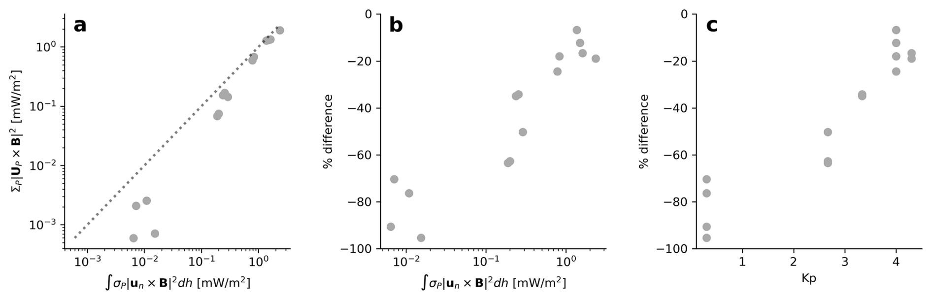
Figure 4 (a) Comparison of the difference between the integral $\int {\mathit{\sigma }}_{\mathrm{P}}\mathrm{|}\mathit{u}\times \mathit{B}{\mathrm{|}}^{\mathrm{2}}\mathrm{d}h$ (last term on RHS of Eq. 10) calculated from altitude profiles of σ_P and u and the lower-bound approximation Σ_P|U_P×B|² calculated from height-integrated quantities. (b) Percent difference between the value of the integral and the lower-bound approximation, relative to the value of the integral. (c) Percent difference as a function of K_p. The point of this figure is to answer Question 3 posed at the beginning of Sect. 3 as to how much the lower-bound approximation calculated from height-integrated quantities underestimates the magnitude of the true integral.

4 Discussion

This study aims to clear up misconceptions about how to incorporate thermospheric winds, which are sparsely sampled, and highly variable and structured in altitude, into IT data assimilation techniques that rely on 2D uniform slabs to describe IT electrodynamics. The assumption of a steady-state force balance between Lorentz and collisional drag forces is central to the expressions for the ionospheric Ohm's law and Joule heating we have used. The accuracy of assumed steady-state stress balance can be assessed by comparing the ion inertial term to the collisional drag term in the ion momentum equation, i.e. by the ratio ${\mathit{\tau }}_{\text{relax}}/{\mathit{\tau }}_{\text{var}}$, where ${\mathit{\tau }}_{\text{relax}}\sim {\mathit{\nu }}_{\text{in}}^{-\mathrm{1}}$ is the ion–neutral relaxation time and τ_var is the characteristic timescale of variability. In the 110–130 km altitude range ν_in is large, making τ_relax of order ∼0.01–0.1 s; here inertial effects become significant only for variability on comparable sub-second timescales. Even under highly active conditions, typical electrodynamic variability occurs on timescales of seconds to minutes, implying that the inertial term is smaller than the drag term by at least an order of magnitude.

Even for fluctuations at several Hz (representative of extreme Alfvénic forcing), the inertial contribution would remain ≲10 % of the drag term, and substantially smaller for more typical variability. Other neglected terms, such as pressure gradients and gravity, are smaller still ($\sim {\mathrm{10}}^{-\mathrm{4}}$ of the drag term). Therefore, in the altitude range where the conductivities maximize, the steady-state balance between Lorentz and collisional drag forces is expected to be accurate to within a few tens of percent under extreme conditions, and considerably more accurate under typical conditions. Thus while transient departures from steady state may occur during highly dynamic events or at very small spatial scales, the quasi-steady approximation we have used is generally robust for describing high-latitude electrodynamics in this altitude range (e.g. Vasyliunas, 2012).

The analysis in Sect. 2 shows how height integration of the ionospheric Ohm's law yields two separate neutral wind vectors (defined by Eq. 9), and that height-integrated variables can only produce a lower-bound estimate of the isolated contribution of neutral winds to Joule heating (third term on the right-hand side of Eq. 10). This analysis has some bearing on the “key MI coupling equation” derived from current continuity that is mentioned in the introduction,

$$\begin{array}{}\text{(12)}& {\displaystyle }{\displaystyle }\mathrm{\nabla }\cdot {\mathit{J}}_{⟂}=-j_{\parallel },\end{array}$$

where the integrated perpendicular current J_⟂ is given by a height- or field line-integrated form of Ohm's law (i.e. ${\mathit{J}}_{⟂}=\overline{\overline{\mathrm{\Sigma }}}\cdot \left[{\mathit{E}}_{⟂}+\mathit{U}\times \mathit{B}\right]$) in terms of an ionospheric conductance tensor $\overline{\overline{\mathrm{\Sigma }}}$, the potential electric field ${\mathit{E}}_{⟂}=-{\mathrm{\nabla }}_{⟂}\mathrm{\Phi }$, and an effective neutral wind U. The development in Sect. 2 shows that it is strictly speaking not possible to formulate the height-integrated ionospheric Ohm's law as given by Eq. (7) in terms of the conductance tensor $\overline{\overline{\mathrm{\Sigma }}}$, because F_H and F_P are generally not identical. However, it is unclear from the results presented in Fig. 3 how much the differences between U_H and U_P might affect the description of IT electrodynamics in models that employ some form of this equation. This topic may be the subject of a future investigation.

Regarding representation of MI coupling in global models, Eq. (12) is not the state of the art: Ionosphere-thermosphere models such as the Whole Atmosphere Community Climate Model With Thermosphere and Ionosphere Extension (WACCM-X, Liu et al., 2018) and the Thermosphere-Ionosphere-Electrodynamics General Circulation Model (Qian et al., 2014) use the 2D continuity equation given in the more advanced treatment of Richmond (1995). The Richmond (1995) equation generalizes Eq. (12) and does, in fact, take stock of the three-dimensional nature of the neutral wind field. Approaches similar to that of Richmond (1995) have also been presented (Maute et al., 2021; Zhu et al., 2022; Laundal et al., 2025b).

The results in Sect. 3 constitute the first experimental comparison of the two neutral wind vectors, showing that with increasing geomagnetic activity the difference in magnitude of these vectors increases (Fig. 2b) while the vectors themselves become more aligned (Fig. 2c). It is nevertheless difficult to draw general conclusions about U_H and U_P solely on the basis of the estimates shown in Fig. 2a, as these estimates are representative of only one location (PFRR) for a sparsely sampled range of universal times (∼06:00–14:00 UT) and one season (January to March), as indicated in Table 1. It nevertheless seems reasonable that the range of magnitudes of U_H and U_P shown in Fig. 2a is typical at high latitudes during low to moderate geomagnetic activity.

Section 3.3 addresses the commonly employed assumption in experimental studies that the winds are zero in Earth's corotating frame of reference, as well as the concept of a two-dimensional “effective neutral wind” pattern introduced by Lu et al. (1995) and employed by both Baker et al. (2004) and Billett et al. (2018). These studies take the effective neutral wind pattern to be the neutral winds at 160 km altitude, u₁₆₀, although analysis in Sect. 2 indicates that a more suitable definition for the effective neutral wind is the Pedersen-weighted neutral wind U_P, which appears in both the height-integrated Ohm's law (Eq. 7) and the lower-bound estimate of Joule heating (Inequality 11).

Given the scarcity of simultaneous measurements of the quantities needed to calculate U_P and U_H (altitude profiles of conductivities and neutral wind), another motivation for this study is to investigate potential proxies for U_P and U_H. Figure 3a explores the accuracy of four proxies for U_P. Statistically speaking, the best proxy for U_P is ${\mathit{u}}_{{\mathit{\sigma }}_{\mathrm{P}}\text{peak}}$, the neutral wind at the altitude of the peak Pedersen conductivity (located between 115 and 128 km altitude for the 15 rocket flights presented in Table 1). In contrast, the proxy for U_H with the lowest median error is the zero vector (pink).

Regardless, all proxies perform similarly in the sense that all are associated with errors of order at least several tens of m s⁻¹. While this result is subject to the same caveat given above regarding limited sampling, it does suggest that one should be skeptical of “quick fixes” for the neutral wind problem, including ignoring the winds or using wind estimates from higher altitudes such as those estimated via Fabry–Perot interferometers attuned to the 630-nm (red) line (e.g. Shiokawa et al., 2014, and references therein), which tend to cover the F-region ionosphere. On the other hand Fabry–Perot interferometers attuned to 557.7 nm (green-line) emissions, which tend to peak between 100 and 130 km altitude, could provide neutral wind estimates relevant for analysis of high-latitude IT electrodynamics. The primary caveat with these measurements is that the peak height of green-line emissions can range over ∼80 to 180 km altitude via the influence of auroral precipitation (Whiter et al., 2023).

Section 3.4 provides an experimental demonstration of the analytic result that the isolated contribution of neutral winds to Joule heating ($\int {\mathit{\sigma }}_{\mathrm{P}}|{\mathit{u}}_n\times \mathit{B}{|}^{\mathrm{2}}\mathrm{d}h$, third term on the right-hand side of Eq. 10) is underestimated when calculated from height-integrated quantities as ${\mathrm{\Sigma }}_{\mathrm{P}}|{\mathit{U}}_{\mathrm{P}}\times \mathit{B}{|}^{\mathrm{2}}$. Figure 4c shows that the contribution estimated from height-integrated quantities tends to approach the true contribution with increasing K_p.

To further illustrate how the neutral wind affects height-integrated Joule heating, each panel in Fig. 5 plots the three terms in Eq. (10) as a function of a hypothetical electric field, assuming the electric field is either perpendicular or parallel to U_P×B (left and right columns, respectively). The values for the neutral wind and Pedersen conductance are taken from the Super Soaker and Auroral Jets campaigns, corresponding respectively to quiet (top row) and active (bottom row) geomagnetic conditions. The total Joule heating (thick gray line) is also plotted in each panel, along with the approximate total Joule heating (dotted gray line) given by replacing the third term $\int {\mathit{\sigma }}_{\mathrm{P}}|{\mathit{u}}_n\times \mathit{B}{|}^{\mathrm{2}}\mathrm{d}h$ with the approximation ${\mathrm{\Sigma }}_{\mathrm{P}}|{\mathit{U}}_{\mathrm{P}}\times \mathit{B}{|}^{\mathrm{2}}$, as in Inequality 11. Electric field values in the top row vary from −10 to 10 mV m⁻¹, and from −50 to 50 mV m⁻¹ in the lower row, corresponding to typical ranges during geomagnetically quiet and active periods (e.g. Walach et al., 2021).

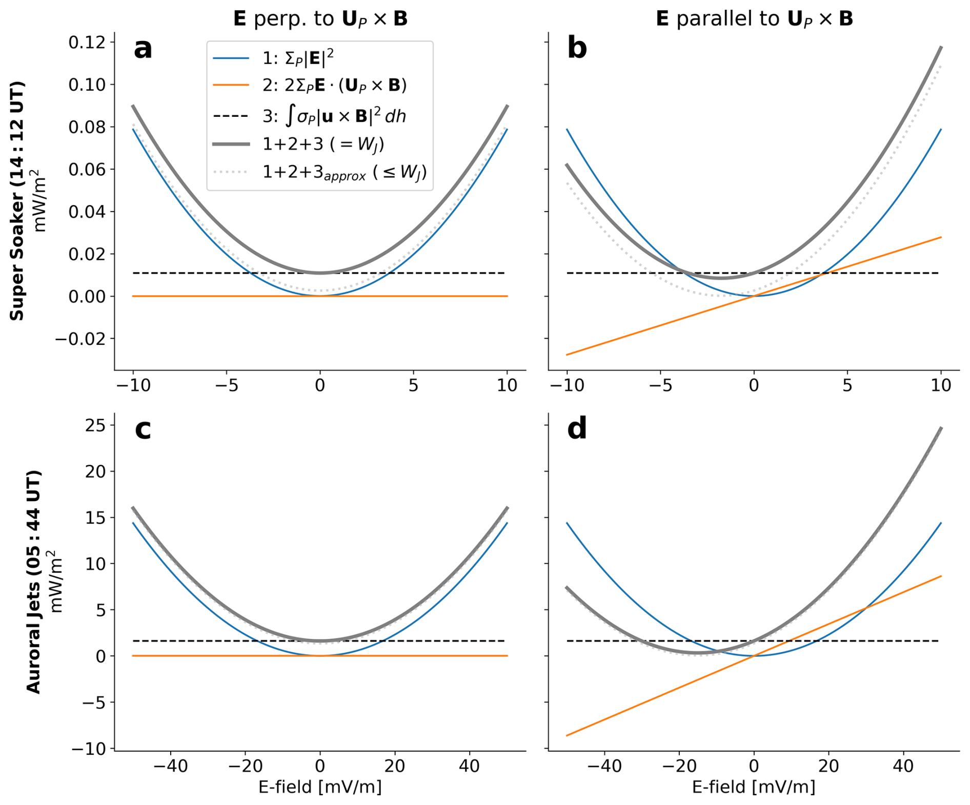
Figure 5 Comparison of terms in Eq. (10) during quiet (top row, Super Soaker campaign) and active (bottom row, Auroral Jets campaign) geomagnetic conditions for a hypothetical electric field that is either perpendicular or parallel to U_P×B (left and right columns, respectively). The blue, orange, and dashed black lines respectively correspond to the first, second, and third terms in Eq. (10). The thick, gray line shows the sum of all three terms, and the dotted gray line shows the sum when the third term ($\int {\mathit{\sigma }}_{\mathrm{P}}|{\mathit{u}}_n\times \mathit{B}{|}^{\mathrm{2}}\mathrm{d}h$) is replaced with the approximation ${\mathrm{\Sigma }}_{\mathrm{P}}|{\mathit{U}}_{\mathrm{P}}\times \mathit{B}{|}^{\mathrm{2}}$. Note that the range of both Joule heating values and electric field values in the bottom row is larger than in the top row.

When the electric field is perpendicular to U_P×B (Fig. 5a and c), the second term (orange line) is zero by definition. In this case, the total Joule heating $W_J={\mathrm{\Sigma }}_{\mathrm{P}}|\mathit{E}{|}^{\mathrm{2}}+\int {\mathit{\sigma }}_{\mathrm{P}}|\mathit{u}\times \mathit{B}{|}^{\mathrm{2}}\mathrm{d}h$. The contribution of the neutral winds is to shift the parabola representing Joule heating upward. That is, the neutral winds make a constant and non-negative contribution to the overall Joule heating. The difference between the true total Joule heating and the approximate total Joule heating, dictated by Inequality 11, can be seen by comparing the thick gray line and dotted gray line that respectively represent them.

When the electric field is parallel to U_P×B (Fig. 5b and d) the situation is more complicated, since the second term offsets total Joule heating via a linear dependence on the electric field. The two cases shown in these panels illustrate that the vertex, or minimum, is shifted horizontally such that it is located at $\mathit{E}=-{\mathit{U}}_{\mathrm{P}}\times \mathit{B}$. The minimum Joule heating value would be zero if the third term $\int {\mathit{\sigma }}_{\mathrm{P}}|{\mathit{u}}_n\times \mathit{B}{|}^{\mathrm{2}}\mathrm{d}h$ were equal to the approximation ${\mathrm{\Sigma }}_{\mathrm{P}}|{\mathit{U}}_{\mathrm{P}}\times \mathit{B}{|}^{\mathrm{2}}$. It is precisely the difference between the true term and its approximation that causes true Joule heating (thick gray line) to be everywhere greater than zero, in agreement with Inequality 11. When the third term is replaced by the approximation ${\mathrm{\Sigma }}_{\mathrm{P}}|{\mathit{U}}_{\mathrm{P}}\times \mathit{B}{|}^{\mathrm{2}}$, the minimum of the approximate total Joule heating (dotted gray lines) is zero as expected.

Two additional general conclusions can be drawn from Fig. 5: (1) During quiet geomagnetic conditions (top row), the neutral wind influences total Joule heating via both its orientation with respect to the convection electric field (second term, horizontal shifting of the parabola) and its magnitude (third term, vertical shifting). (2) During active conditions (bottom row), the magnitude of the neutral wind is likely less important, with its primary influence being to reduce or enhance the the total Joule heating. This can most easily be seen in Fig. 5 as the difference between the parabola that defines the total Joule heating (thick gray line) and the parabola that defines the first term (blue line).

In summary, in this study we have pointed out a fundamental limitation of 2D descriptions of IT electrodynamics: In a 2D representation, the governing equation (ionospheric Ohm's law) contains two neutral wind terms that are separately weighted by the altitude profiles of Hall and Pedersen conductivities. Furthermore, even when an appropriately defined neutral wind term is used (the Pedersen-weighted neutral wind), any estimate of height-integrated Joule heating on the basis of height-integrated and averaged quantities is mathematically guaranteed to be a lower bound of the actual height-integrated Joule heating, with some tendency for the pure neutral wind term to be less strongly underestimated with increasing K_p.

At a basic level this study is one more voice in the chorus of recent literature calling for additional neutral wind measurements (Sarris, 2019; Heelis and Maute, 2020; Palmroth et al., 2021; Dhadly et al., 2023). However, results in Fig. 3 show that estimates of height-integrated electrodynamic quantities might be improved simply by having an estimate of the neutral wind at a single altitude near the altitude at which the Pedersen conductivity peaks. This points to the utility of techniques and measurements that enable estimation of the neutral wind profiles over limited ranges of altitudes between 120–200 km where the Pedersen conductivity profile may peak, including Doppler spectroscopy based on emissions from atomic oxygen at 558 nm (Branning et al., 2022; Dhadly et al., 2023, and references there in) as well as next-generation incoherent scatter radar systems such as PFISR and the upcoming EISCAT_3D facility (Zhan and Kaeppler, 2025; Reistad et al., 2024, and references therein).

It remains to be seen how important the distinction between the Hall- and Pedersen-weighted neutral winds is for calculations of the height-integrated current density as given by Eq. (7). It likewise remains to be seen whether estimates of the Hall and Pedersen conductances on the basis of estimates of the height-integrated perpendicular current and electric field, as is done by Weimer and Edwards (2021) and Hatch et al. (2024), can be improved by inclusion of limited information about the neutral winds. We suggest that it would be valuable to compare height-integrated Joule heating estimated directly from altitude profiles (Eq. 10) and from height-integrated variables (Eq. 4), and to carry out similar comparisons for height-integrated current density (Eq. 1 vs. Eq. 7) and conductance ($\int {\mathit{\sigma }}_{\mathrm{H},\mathrm{P}}\mathrm{d}h$ vs. Eq. 3). Such a study would be experimentally very demanding, as it would require comprehensive information about the state of the coupled ionosphere-thermosphere system.

Appendix A: Relationship between assumed E-field height independence and scale size of variations

Here we briefly show how one effectually assumes a limit on the scale size of variations of E_⟂ across field lines by assuming E_⟂ does not vary with altitude.

Suppose magnetic field lines are locally tilted by an angle θ relative to the vertical direction (i.e. inclination $I=\mathrm{90}\mathit{°}-\mathit{\theta }$), and that we have a coordinate system $x^{\prime }y{z}^{\prime }$ that is such that z^′ is parallel to field lines locally and x^′ and y are perpendicular. This coordinate system is tilted relative to a local xyz coordinate system, with the x direction of the latter determined by ensuring that the field lines are contained within the xz plane and the z direction upward. The transformations from xyz to $x^{\prime }y{z}^{\prime }$ coordinates are then

$$\begin{array}{l}{\displaystyle }{x}^{\prime }=x\cos \mathit{\theta }-z\sin \mathit{\theta };\\ {\displaystyle }{z}^{\prime }=x\sin \mathit{\theta }+z\cos \mathit{\theta }.\end{array}$$

The perpendicular electric field ${\mathit{E}}_{⟂}\left(x^{\prime },y\right)={\mathit{E}}_{⟂}\left(x\cos \mathit{\theta }-z\sin \mathit{\theta },y\right)=E_{⟂,x^{\prime }}{\widehat{\mathit{x}}}^{\prime }+E_{⟂,y}\widehat{\mathit{y}}$.

We now examine the integral over height of the first term on the right-hand side of Eq. (1),

$$\begin{array}{}\text{(A1)}& {\displaystyle }{\displaystyle }\underset{z_{\mathrm{1}}}{\overset{z_{\mathrm{2}}}{\int }}{\mathit{\sigma }}_{\mathrm{P}}\left(z\right){\mathit{E}}_{⟂}\left(x\cos \mathit{\theta }-z\sin \mathit{\theta },y\right)\mathrm{d}z,\end{array}$$

where for simplicity we take u=0. Moving E_⟂ outside the integral requires that E_⟂ be approximately invariant between z₁ and z₂, or equivalently (via the dependence of E_⟂ on x^′) over a horizontal distance $d=(z_{\mathrm{2}}-z_{\mathrm{1}})\tan \mathit{\theta }$. For example, if the local field inclination I=70° and the effective vertical extent of the ionosphere ${\mathrm{\Delta }}_z=z_{\mathrm{2}}-z_{\mathrm{1}}=\mathrm{50}$ km, assuming E_⟂ does not vary with altitude is equivalent to assuming that it does not vary over a distance d≈18 km, or about 0.2°. The situation is more drastic in the Southern Hemisphere, where if the inclination I=50° the distance is ∼30 km, or 0.3°.

Thus one effectually assumes a limit on the scale size of variations of E_⟂ across field lines by assuming E_⟂ does not vary with altitude. An example of where this could be taken into account is given in the text immediately following Eq. (9) in Aikio et al. (2012).

Appendix B: Cauchy–Bunyakovsky–Schwarz proof

Let $L_w^{\mathrm{2}}(X,\mathit{\mu })$ be a weighted L² space over X with measure μ. The corresponding inner product for functions f and g is

$$\begin{array}{}\text{(B1)}& {\displaystyle }{\displaystyle }\langle f,g\rangle =\underset{X}{\int }f\left(t\right)\stackrel{\mathrm{‾}}{g\left(t\right)}w\left(t\right)\mathrm{d}t,\end{array}$$

with w(t)>0 for all t. The inner product (Eq. B1) obeys the Cauchy–Bunyakovsky–Schwarz inequality

$${\displaystyle }{\left|\langle f,g\rangle \right|}^{\mathrm{2}}\le \langle f,f\rangle \langle g,g\rangle .$$

Taking f=1, g=u_i (the i^th component of the neutral wind u), and μ=σ_P, we have

$${\displaystyle }{\left|\int {\mathit{\sigma }}_{\mathrm{P}}{u}_i\mathrm{d}h\right|}^{\mathrm{2}}={\mathrm{\Sigma }}_{\mathrm{P}}^{\mathrm{2}}{U}_{\mathrm{P},i}^{\mathrm{2}}\le {\mathrm{\Sigma }}_{\mathrm{P}}\int {\mathit{\sigma }}_{\mathrm{P}}{u}_i^{\mathrm{2}}\mathrm{d}h,$$

or rearranging,

$${\displaystyle }\int {\mathit{\sigma }}_{\mathrm{P}}{u}_i^{\mathrm{2}}\mathrm{d}h\ge {\mathrm{\Sigma }}_{\mathrm{P}}{U}_{\mathrm{P},i}^{\mathrm{2}}.$$

Summing this inequality for each component of u we find

$$\begin{array}{}\text{(B2)}& {\displaystyle }{\displaystyle }\int {\mathit{\sigma }}_{\mathrm{P}}\mathrm{|}\mathit{u}{\mathrm{|}}^{\mathrm{2}}\mathrm{d}h\ge {\mathrm{\Sigma }}_{\mathrm{P}}\mathrm{|}{\mathit{U}}_{\mathrm{P}}{\mathrm{|}}^{\mathrm{2}}.\end{array}$$

If in addition the magnetic field B is approximately constant between altitudes of ∼80–200 km, then multiplying both sides of Inequality B2 by |Bsin θ|² and applying the geometric definition of the cross product ($\mathrm{|}\mathit{u}\mathrm{|}\mathrm{|}\mathit{B}\mathrm{|}\sin \mathit{\theta }=\mathit{u}\times \mathit{B}$) we have

$$\begin{array}{}\text{(B3)}& {\displaystyle }{\displaystyle }\int {\mathit{\sigma }}_{\mathrm{P}}\mathrm{|}\mathit{u}\times \mathit{B}{\mathrm{|}}^{\mathrm{2}}\mathrm{d}h\ge {\mathrm{\Sigma }}_{\mathrm{P}}\mathrm{|}{\mathit{U}}_{\mathrm{P}}\times \mathit{B}{\mathrm{|}}^{\mathrm{2}}.\end{array}$$

Appendix C: Calculation of conductivity profiles

Hall and Pedersen conductivity profiles σ_H and σ_P are derived following Ieda (2020), with

$$\begin{array}{}\text{(C1)}& {\displaystyle }{\displaystyle }\left({\mathit{\sigma }}_{\mathrm{H}},{\mathit{\sigma }}_{\mathrm{P}}\right)=\left({\mathit{\sigma }}_{\mathrm{H},e}-{\mathit{\sigma }}_{\mathrm{H},i},{\mathit{\sigma }}_{\mathrm{P},e}+{\mathit{\sigma }}_{\mathrm{P},i}\right).\end{array}$$

Subscripts e and i refer to the contributions from electrons and ions. For each conductivity the ion contribution is a sum over ion species:

$$\begin{array}{}\text{(C2)}& {\displaystyle }{\displaystyle }{\mathit{\sigma }}_{\mathit{\{}\mathrm{H},\mathrm{P}\mathit{\}},i}=\sum _{l={\mathrm{NO}}^{+},{\mathrm{O}}_{\mathrm{2}}^{+},{\mathrm{O}}^{+}}{\mathit{\sigma }}_{\mathit{\{}\mathrm{H},\mathrm{P}\mathit{\}},l}.\end{array}$$

The contribution from each charged particle species j (NO⁺, ${\mathrm{O}}_{\mathrm{2}}^{+}$, O⁺, and e⁻) is given by

$$\begin{array}{}\text{(C3)}& {\displaystyle }{\displaystyle }\left({\mathit{\sigma }}_{\mathrm{H},j},{\mathit{\sigma }}_{\mathrm{P},j}\right)={\displaystyle \frac{e{n}_j}{B}}\left({\displaystyle \frac{k_j^{\mathrm{2}}}{\mathrm{1}+k_j^{\mathrm{2}}}},{\displaystyle \frac{k_j}{\mathrm{1}+k_j^{\mathrm{2}}}}\right),\end{array}$$

with $k_j={\mathrm{\Omega }}_j/{\mathit{\nu }}_{jn}$, and Ω_j and ν_jn respectively the gyrofrequency and collision frequency for momentum transfer between charged particle species j and neutrals.

Expressions for ν_jn are given in Appendix A of Ieda (2020) for the three ion species just mentioned and neutral species N₂, O₂, and O. These expressions take stock of non-resonant collisions between parental pairs such as ${\mathrm{O}}_{\mathrm{2}}^{+}$ and O₂ that are neglected by, for example, Schunk and Nagy (2009), but are nevertheless an essential part of the description of ion-neutral collisions for ion and neutral temperatures below approximately 600 K.

Figure C1 illustrates the quantities involved in the calculation of conductivity for a wind profile measured during the Mesospheric Inversion Layer Stratified Turbulence (MIST) campaign on 26 January 2015. In Fig. C1a densities of neutral species are given by the NRLMSIS^® 2.0 empirical atmospheric model (Emmert et al., 2020). In Fig. C1b the electron density (labeled e⁻) is measured by PFISR, and the ion species densities are given by multiplying the electron density by the fractional composition of each species as given by the International Reference Ionosphere (IRI) 2016 model (Bilitza et al., 2017). In Fig. C1c the electron and ion temperatures are measured by PFISR, and the neutral temperature is given by IRI 2016.

From these density and temperature profiles we calculate collision frequencies (Fig. C1d) and conductivity profiles (Fig. C1e) that are ultimately used to estimate the zonal (labeled U_H and U_P) and meridional (labeled V_H and V_P) components of the Hall- and Pedersen-weighted neutral winds, which are indicated with vertical lines in Fig. C1f. The Supplement contains figures corresponding to Fig. C1 for the remaining 14 wind profiles.

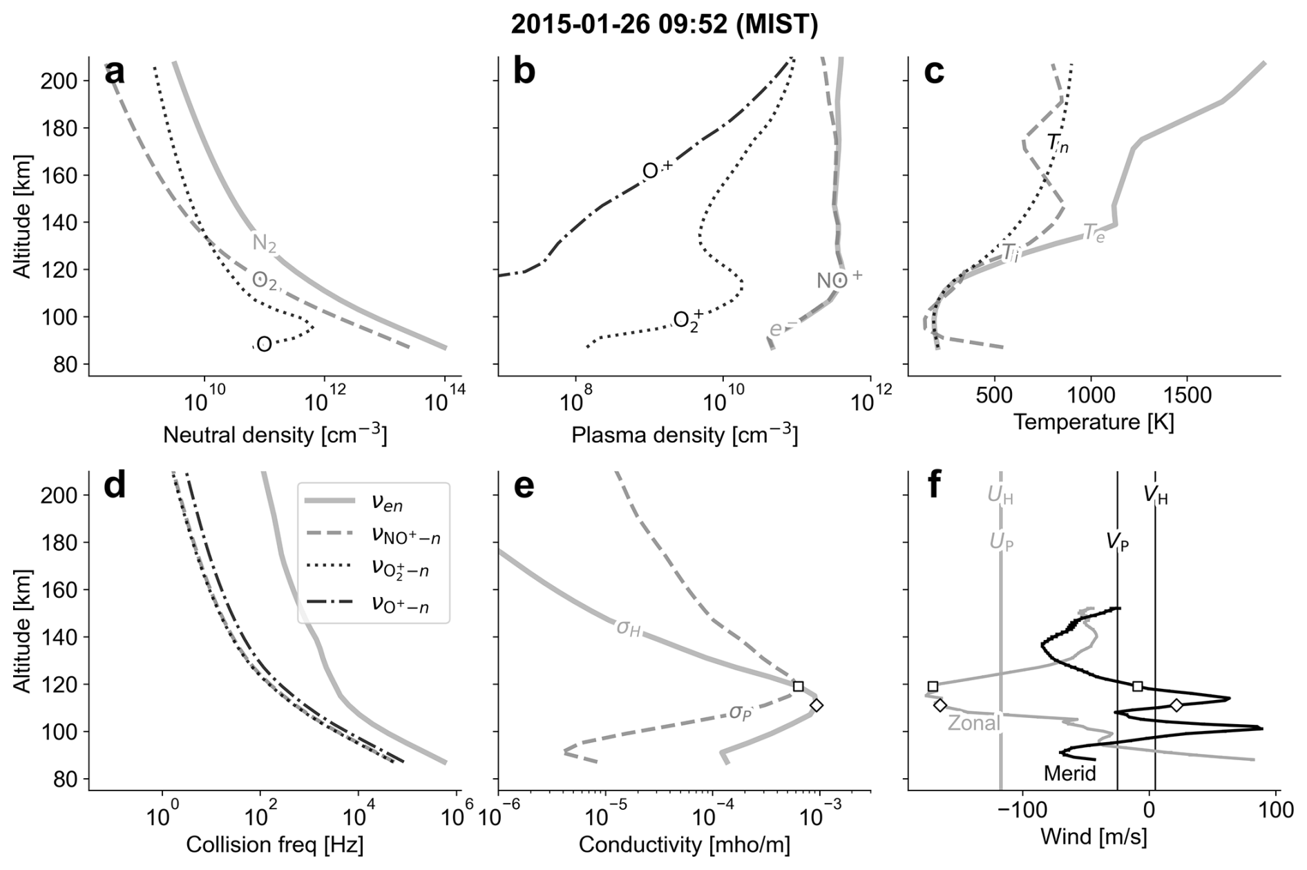
Figure C1 Illustration of altitude profiles needed for calculation of zonal and meridional components of the Hall- and Pedersen-weighted winds via Eq. (9). These profiles correspond to the MIST rocket launched 26 January 2015 09:52 UT during moderate geomagnetic activity (K_p=4.0; see Fig. 1c1–c3). (a) Neutral density profiles from NRLMSIS^® 2.0 model. (b) PFISR plasma density profile (e⁻) with fractional ion species densities given by IRI 2016. (c) PFISR electron and ion temperature profiles, and IRI 2016 neutral temperature profile. (d) Ion-neutral collision frequencies calculated from profiles in panels (a–c). (e) Hall and Pedersen conductivity profiles (solid and dashed lines). The peaks of the Hall and Pedersen conductivity profiles are respectively indicated by a diamond and a square. (f) Neutral wind profiles. Zonal (U_H and U_P) and meridional (V_H and V_P) components of the Hall- and Pedersen-weighted neutral winds are indicated with vertical lines. Neutral wind components at peaks of the Hall and Pedersen conductivity profiles respectively also indicated by diamond and square symbols.