Evanescent acoustic-gravity modes in the isothermal atmosphere: systematization and applications to the Earth and solar atmospheres

The objects of research in this work are evanescent wave modes in a gravitationally stratified atmosphere and their associated pseudo-modes. Whereas the former, according to the dispersion relation, rapidly decrease with distance from a certain surface, the latter, having the same dispersion law, differ from the first by the form of polarization and the nature of decrease from the surface. Within a linear hydrodynamic model, the propagation features of evanescent wave modes in an isothermal atmosphere are studied. Research is carried out for different assumptions about the properties of the disturbances. In this way, a new wave mode – anelastic evanescent wave mode – was discovered that satisfies the dispersion relation ${\mathit{\omega }}^{\mathrm{2}}=k_{x}g\left(\mathit{\gamma }-\mathrm{1}\right)$. Also, the possibility of the existence of a pseudo-mode related to it is indicated. The case of two isothermal media differing in temperature at the interface is studied in detail. It is shown that a non-divergent pseudo-mode with a horizontal scale $k_x\sim \mathrm{1}/\mathrm{2}{H}_{\mathrm{1}}$ can be realized on the interface with dispersion ω²=k_xg. Dispersion relation ${\mathit{\omega }}^{\mathrm{2}}=k_{x}g\left(\mathit{\gamma }-\mathrm{1}\right)$ at the interface of two media is satisfied by the wave mode, which has different types of amplitude versus height dependencies at different horizontal scales k_x. The applicability of the obtained results to clarify the properties of the f-mode observed on the Sun is analyzed.

1 Introduction

Acoustic-gravity waves (AGWs) in the Earth's atmosphere have been studied theoretically and experimentally for more than 60 years. The linear theory of AGW (Hines, 1960; Yeh and Liu, 1974; Francis, 1975) admits the existence in the atmosphere of a continuous spectrum of freely propagating waves, consisting of acoustic and gravity regions on the dispersion plane, as well as of evanescent modes, which can only propagate horizontally.

The freely propagating AGWs effectively transfer the energy and momentum between various atmospheric layers and thus play an important role in the dynamics and energy balance of the atmosphere. These waves are generated by various sources (both natural and technogenic ones), which are accompanied by a significant energy output into the atmosphere. Further, when the AGWs propagate upward, the energy conservation compensates for the decrease in the atmospheric density with the height by exponentially increasing amplitude. Therefore at a certain height the waves become nonlinear. Significant progress in the development of the nonlinear theory of AGWs was achieved by a number of authors, in particular, Belashov (1990), Nekrasov et al. (1995), Kaladze et al. (2008), Stenflo and Shukla (2009), and Huang et al. (2014). Numerical modeling of the freely propagating AGWs in the realistic viscous and heat-conducting atmosphere is an important area of modern studies of these waves (i.e., Cheremnykh et al., 2010; Vadas and Nicolls, 2012).

Satellite observations of AGWs in the Earth's polar thermosphere indicate a prevailing presence of waves with oscillation periods concentrated around the Brunt–Väisälä period and of horizontal scales of about 500–700 km (Johnson et al., 1995; Innis and Conde, 2002; Fedorenko et al., 2015). Azimuths of the propagation of these AGWs demonstrate the close connection with the directions of background winds in the thermosphere. Moreover, the amplitudes of the waves depend on the speed of headwind, but do not depend on height (Fedorenko and Kryuchkov, 2013; Fedorenko et al., 2018). These experimental results cannot be sufficiently explained by the theory of freely propagating AGWs. They may indicate waveguide or evanescent (along a horizontal surface) propagation of at least part of the observed waves.

As well as freely propagating AGWs, evanescent wave modes also play an important role in atmospheric dynamics of the Sun and planets. Evanescent waves propagate horizontally in an atmosphere, vertically stratified by gravity, subject to the presence of vertical gradients of parameters. The energy of these waves should decrease both up and down from the level at which they are generated. Therefore, evanescent waves are most effectively generated in areas of presence of significant vertical gradients of temperature and density or strong local currents. For example, in the solar atmosphere suitable conditions for realization of evanescent modes occur at the boundary between the chromosphere and corona. This follows from the analysis made by Jones (1969) for the so-called non-divergent modes of solar oscillations. In the Earth's atmosphere, such waves can be efficiently generated at sharp vertical temperature gradients, for example, at the base of the thermosphere or at the heights of the tropopause and mesopause. Also, evanescent wave modes can emerge in the presence of strong inhomogeneous winds, for example, in the region of the polar circulation of the thermosphere.

The study of evanescent waves traditionally gets less attention than the study of freely propagating AGWs. The most known of them are the horizontal Lamb wave and vertical oscillations with Brunt–Väisälä (BV) frequency (Beer, 1974; Waltercheid and Hecht, 2003). In hydrodynamics, physics of terrestrial and solar atmosphere, the surface gravity mode with dispersion ω²=k_xg, is also well studied (Tolstoy, 1963; Jones, 1969). In particular, it was shown that it is the fundamental mode (f-mode) of oscillations in the solar atmosphere (Jones, 1969). Experimental f-mode observations are used to study flows, refinement of the solar radius, and other parameters of the Sun (Ghosh et al., 1995; Antia, 1998). In the Earth's atmosphere, evanescent waves are often observed at altitudes near the mesopause using ground-based instrumentation (Shimkhada et al., 2009).

In this paper, different types of evanescent acoustic-gravity modes characteristic of an isothermal atmosphere are investigated using a set of linearized hydrodynamic equations. In particular, the possibility of the existence of a new type of evanescent acoustic-gravity mode with the dispersion ${\mathit{\omega }}^{\mathrm{2}}=k_{x}g\left(\mathit{\gamma }-\mathrm{1}\right)$ is proved in the assumption of anelasticity of the disturbance. Also, the possibility of realizing the evanescent modes in the model of a thin temperature gap is studied.

2 Evanescent modes in the isothermal atmosphere

Consider an unbounded ideal isothermal atmosphere, stratified in a field of gravity. Linear perturbations in such a medium satisfy a set of four first-order hydrodynamic equations (Hines, 1960). These equations are convenient to bring to a set of two second-order equations for the perturbations of the horizontal V_x and vertical V_z particle velocities (Tolstoy, 1963):

$$\begin{array}{}\text{(1)}& {\displaystyle }& {\displaystyle }{\mathit{\rho }}_{\mathrm{0}}{\displaystyle \frac{{\partial }^{\mathrm{2}}{V}_x}{\partial t^{\mathrm{2}}}}=-{\mathit{\rho }}_{\mathrm{0}}g{\displaystyle \frac{\partial V_z}{\partial x}}+{\displaystyle \frac{\partial }{\partial x}}\left[{\mathit{\rho }}_{\mathrm{0}}{c}^{\mathrm{2}}\left({\displaystyle \frac{\partial V_x}{\partial x}}+{\displaystyle \frac{\partial V_z}{\partial z}}\right)\right],\text{(2)}& {\displaystyle }& {\displaystyle }{\mathit{\rho }}_{\mathrm{0}}{\displaystyle \frac{{\partial }^{\mathrm{2}}{V}_z}{\partial t^{\mathrm{2}}}}={\mathit{\rho }}_{\mathrm{0}}g{\displaystyle \frac{\partial V_x}{\partial x}}+{\displaystyle \frac{\partial }{\partial z}}\left[{\mathit{\rho }}_{\mathrm{0}}{c}^{\mathrm{2}}\left({\displaystyle \frac{\partial V_x}{\partial x}}+{\displaystyle \frac{\partial V_z}{\partial z}}\right)\right],\end{array}$$

where ρ₀, γ, and g denote background atmosphere density, ratio of specific heats, and acceleration of gravity, respectively; $c=\sqrt{\mathit{\gamma }gH}$ is the sound speed, $H=-{\mathit{\rho }}_{\mathrm{0}}/\left(d{\mathit{\rho }}_{\mathrm{0}}/\mathrm{d}z\right)=kT/mg$ is the density-scale height, T is the temperature, k is the Boltzmann constant, and m is the molecular mass of the atmospheric gas.

Solutions to Eqs. (1) and (2) are searched for in the form

$$\begin{array}{}\text{(3)}& V_x,V_z\sim \exp \left(az\right)\exp \left[i\left(\mathit{\omega }t-k_{x}x\right)\right],\end{array}$$

where ω and k_x are cyclic frequency and horizontal component of the wave vector, respectively; parameter a sets the vertical scale of the change in the amplitude of velocities, V_x and V_z, with the height, z. For brevity, we will refer to a as the stratification of the corresponding mode.

Equations (1) and (2) admit, similarly to Hines (1960), on the existence on the “frequency–wave number” plot of regions of freely propagating gravity and acoustic waves, in which $a=\frac{\mathrm{1}}{\mathrm{2}H}\pm i{k}_z$ and k_z is the vertical component of the wave vector. Also, from Eqs. (1) and (2) we get the solutions in the form of evanescent wave modes with real a and propagating horizontally (Waltercheid and Hecht, 2003). Solutions in the form of evanescent modes are usually obtained by imposing additional conditions on the perturbation properties.

2.1 Non-divergent and pseudo-non-divergent modes

Let us note the well-known hydrodynamics approximation of perturbations incompressibility (see, e.g., Ladikov-Roev and Cheremnykh, 2010), for which

$$\begin{array}{}\text{(4)}& \mathrm{div}\mathit{V}={\displaystyle \frac{\partial V_x}{\partial x}}+{\displaystyle \frac{\partial V_z}{\partial z}}=\mathrm{0}.\end{array}$$

In frames of this approximation, we obtain the following equations from Eqs. (1) and (2):

$$\begin{array}{}\text{(5)}& {\displaystyle }& {\displaystyle \frac{{\partial }^{\mathrm{2}}{V}_x}{\partial t^{\mathrm{2}}}}=-g{\displaystyle \frac{\partial V_z}{\partial x}},\text{(6)}& {\displaystyle }& {\displaystyle \frac{{\partial }^{\mathrm{2}}{V}_z}{\partial t^{\mathrm{2}}}}=g{\displaystyle \frac{\partial V_x}{\partial x}}.\end{array}$$

After substituting Eq. (3) into Eqs. (5) and (6), we find that

$$\begin{array}{ll}{\displaystyle }& {\displaystyle }-{\mathit{\omega }}^{\mathrm{2}}{V}_x=i{k}_{x}g{V}_z,\\ {\displaystyle }& {\displaystyle }-{\mathit{\omega }}^{\mathrm{2}}{V}_z=-i{k}_{x}g{V}_x.\end{array}$$

This yields a dispersion equation for incompressible wave modes in the form

$$\begin{array}{}\text{(7)}& {\mathit{\omega }}^{\mathrm{2}}=k_{x}g.\end{array}$$

Given the dispersion found, we obtain an expression for the polarization of the incompressible modes:

$$\begin{array}{}\text{(8)}& V_z=i{V}_x.\end{array}$$

Further, from the condition (Eq. 4) and polarization (Eq. 8) we get a=k_x. Insofar as a is a real value, then non-divergent (ND) wave mode has no periodic vertical solution and is horizontally propagating.

Let us show that the dispersion relation (Eq. 7) is also satisfied by another wave mode. After using this relation in Eqs. (1) and (2), we get

$$\begin{array}{}\text{(9)}& {\displaystyle }& {\displaystyle }{V}_x\left(\mathit{\gamma }H{k}_x-\mathrm{1}\right)-i{V}_z\left(\mathrm{1}-\mathit{\gamma }aH\right)=\mathrm{0},\text{(10)}& {\displaystyle }& {\displaystyle }i{V}_x\left(\mathrm{1}-\mathit{\gamma }Ha-\mathit{\gamma }\right)-V_z\left(\mathrm{1}+{\displaystyle \frac{\mathit{\gamma }H{a}^{\mathrm{2}}}{k_x}}-{\displaystyle \frac{\mathit{\gamma }a}{k_x}}\right)=\mathrm{0}.\end{array}$$

From Eqs. (9) and (10) follow

$${\displaystyle }{a}^{\mathrm{2}}-{\displaystyle \frac{a}{H}}+{\displaystyle \frac{k_x}{H}}\left(\mathrm{1}-k_{x}H\right)=\mathrm{0},$$

which implies that there are two solutions to this equation:

$$\begin{array}{}\text{(11)}& a=k_x,a={\displaystyle \frac{\mathrm{1}}{H}}-k_x.\end{array}$$

The first solution in Eq. (11) corresponds to the non-divergent (ND) wave mode, and the second one we call pseudo-non-divergent mode (NDp). The expression for polarization NDp is obtained from Eq. (9) and has the form

$${\displaystyle }{V}_x\left({\displaystyle \frac{\mathrm{1}}{\mathit{\gamma }H}}-k_x\right)=-i\left(k_x-{\displaystyle \frac{\mathit{\gamma }-\mathrm{1}}{\mathit{\gamma }H}}\right)V_z.$$

Also for this mode, the following equation holds:

$${\displaystyle }\mathrm{div}\mathit{V}={\displaystyle \frac{V_z}{H}}{\displaystyle \frac{\left(\mathrm{1}-\mathrm{2}{k}_{x}H\right)}{\left(\mathrm{1}-\mathit{\gamma }{k}_{x}H\right)}},$$

which shows that for the NDp mode divV=0 only when $k_x=\mathrm{1}/\mathrm{2}H$.

2.2 Anelastic and pseudo-anelastic modes

Let us show that Eqs. (1) and (2) indicate that another wave mode, not previously studied, may exist. To do this, we introduce, according to Bannon (1996), the anelastic linear perturbations, which satisfy the condition

$$\begin{array}{}\text{(12)}& \mathrm{div}\left({\mathit{\rho }}_{\mathrm{0}}\mathit{V}\right)=\mathrm{0}.\end{array}$$

In the isothermal atmosphere with barometric density distribution we have

$${\displaystyle \frac{\partial {\mathit{\rho }}_{\mathrm{0}}}{\partial z}}=-{\displaystyle \frac{{\mathit{\rho }}_{\mathrm{0}}}{H}};$$

therefore, for such anelastic perturbations, the following equation holds:

$$\begin{array}{}\text{(13)}& \mathrm{div}\mathit{V}={\displaystyle \frac{V_z}{H}}.\end{array}$$

Substituting Eq. (13) into Eqs. (1) and (2), we get

$$\begin{array}{ll}{\displaystyle }& {\displaystyle \frac{{\partial }^{\mathrm{2}}{V}_x}{\partial t^{\mathrm{2}}}}=g\left(\mathit{\gamma }-\mathrm{1}\right){\displaystyle \frac{\partial V_z}{\partial x}},\\ {\displaystyle }& {\displaystyle \frac{{\partial }^{\mathrm{2}}{V}_z}{\partial t^{\mathrm{2}}}}=-g\left(\mathit{\gamma }-\mathrm{1}\right){\displaystyle \frac{\partial V_x}{\partial x}}.\end{array}$$

Thus, given Eq. (3), this should be

$$\begin{array}{}\text{(14)}& {\displaystyle }& {\displaystyle }{\mathit{\omega }}^{\mathrm{2}}{V}_x=i{k}_{x}g\left(\mathit{\gamma }-\mathrm{1}\right)V_z,\text{(15)}& {\displaystyle }& {\displaystyle }{\mathit{\omega }}^{\mathrm{2}}{V}_z=-i{k}_x\left(\mathit{\gamma }-\mathrm{1}\right)g{V}_x.\end{array}$$

Then the dispersion equation for anelastic (AE) modes takes the form

$$\begin{array}{}\text{(16)}& {\mathit{\omega }}^{\mathrm{2}}=k_{x}g\left(\mathit{\gamma }-\mathrm{1}\right).\end{array}$$

With the resulting dispersion, polarization follows from Eqs. (14) and (15):

$$\begin{array}{}\text{(17)}& V_x=i{V}_z.\end{array}$$

Further, taking into account Eq. (13), we obtain $a=\frac{\mathrm{1}}{H}-k_x$. Consequently, the AE mode also does not have a solution periodic vertically and can only propagate horizontally.

After substituting the dispersion (Eq. 16) into Eqs. (1) and (2), we get

$$\begin{array}{}\text{(18)}& {\displaystyle }& {\displaystyle }{V}_x\left(\mathrm{1}-\mathit{\gamma }+\mathit{\gamma }H{k}_x\right)-i{V}_z\left(\mathrm{1}-\mathit{\gamma }aH\right)=\mathrm{0},\text{(19)}& {\displaystyle }& {\displaystyle }i{V}_x\left(\mathrm{1}-\mathit{\gamma }+\mathit{\gamma }Ha\right)+V_z\left(\mathrm{1}-\mathit{\gamma }-{\displaystyle \frac{\mathit{\gamma }H{a}^{\mathrm{2}}}{k_x}}+{\displaystyle \frac{\mathit{\gamma }a}{k_x}}\right)=\mathrm{0},\end{array}$$

whence we get a pair of values a identical to Eq. (11). Consequently, there is another wave solution that satisfies Eq. (16): we call it the pseudo-anelastic (AEp) mode. The first value in Eq. (11) corresponds to the AEp wave mode, and the second to the AE one.

Polarization of the AEp mode has the form

$${\displaystyle }{V}_x\left(k_x-{\displaystyle \frac{\mathit{\gamma }-\mathrm{1}}{\mathit{\gamma }H}}\right)=-i\left({\displaystyle \frac{\mathrm{1}}{\mathit{\gamma }H}}-k_x\right)V_z$$

that follows from Eqs. (18) or (19).

3 General properties of evanescent modes

Let us prove that the different types of evanescent modes characteristic of an isothermal atmosphere are related. We substitute Eq. (3) into Eqs. (1) and (2) without additional conditions that were imposed in Sect. 2 when deriving ND and AE modes. As a result, we get

$$\begin{array}{}\text{(20)}& {\displaystyle }& {\displaystyle }{V}_z\left(a-{\displaystyle \frac{g}{c^{\mathrm{2}}}}\right)-i{k}_x{V}_x\left(\mathrm{1}-{\displaystyle \frac{{\mathit{\omega }}^{\mathrm{2}}}{k_x^{\mathrm{2}}{c}^{\mathrm{2}}}}\right)=\mathrm{0},\text{(21)}& {\displaystyle }& {\displaystyle }{V}_x\left(a-{\displaystyle \frac{N^{\mathrm{2}}}{g}}\right)-i{k}_x{V}_z\left({\displaystyle \frac{N^{\mathrm{2}}}{{\mathit{\omega }}^{\mathrm{2}}}}-\mathrm{1}\right)=\mathrm{0},\end{array}$$

where $N^{\mathrm{2}}=\frac{g}{H}\frac{\left(\mathit{\gamma }-\mathrm{1}\right)}{\mathit{\gamma }}$ is the square of the Brunt–Väisälä frequency.

From Eqs. (20) and (21) we obtain the dispersion equation

$$\begin{array}{}\text{(22)}& \left({\displaystyle \frac{\mathrm{1}}{\mathit{\gamma }H}}-a\right)\left(a-{\displaystyle \frac{\mathit{\gamma }-\mathrm{1}}{\mathit{\gamma }H}}\right)=k_x^{\mathrm{2}}\left({\displaystyle \frac{N^{\mathrm{2}}}{{\mathit{\omega }}^{\mathrm{2}}}}-\mathrm{1}\right)\left(\mathrm{1}-{\displaystyle \frac{{\mathit{\omega }}^{\mathrm{2}}}{k_x^{\mathrm{2}}{c}^{\mathrm{2}}}}\right).\end{array}$$

Expressions ω²=N² and ${\mathit{\omega }}^{\mathrm{2}}=k_x^{\mathrm{2}}{c}^{\mathrm{2}}$ are well-known dispersions of Brunt–Väisälä oscillations with $a=\mathrm{1}/\mathit{\gamma }H$ and Lamb waves (L) with $a=\left(\mathit{\gamma }-\mathrm{1}\right)/\mathit{\gamma }H$; in addition to these known modes, dispersion (Eq. 22) also admits the existence of additional solutions in the form of BV pseudo-modes (BVp) with ω²=N², $a=\left(\mathit{\gamma }-\mathrm{1}\right)/\mathit{\gamma }H$ and Lamb pseudo-modes (Lp) with ${\mathit{\omega }}^{\mathrm{2}}=k_x^{\mathrm{2}}{c}^{\mathrm{2}}$, $a=\mathrm{1}/\mathit{\gamma }H$ (Beer, 1974; Waltercheid and Hecht, 2003).

Then represent Eq. (22) in the form of a quadratic equation with respect to a:

$${\displaystyle }{a}^{\mathrm{2}}-{\displaystyle \frac{a}{H}}+{\displaystyle \frac{{\mathit{\omega }}^{\mathrm{2}}}{c^{\mathrm{2}}}}-k_x^{\mathrm{2}}+{\displaystyle \frac{k_x^{\mathrm{2}}{g}^{\mathrm{2}}}{{\mathit{\omega }}^{\mathrm{2}}{c}^{\mathrm{2}}}}\left(\mathit{\gamma }-\mathrm{1}\right)=\mathrm{0}.$$

The solution to this equation is

$$\begin{array}{}\text{(23)}& a={\displaystyle \frac{\mathrm{1}}{\mathrm{2}H}}\pm \sqrt{{\displaystyle \frac{\left(k_{x}g-{\mathit{\omega }}^{\mathrm{2}}\right)\left({\mathit{\omega }}^{\mathrm{2}}-k_{x}g\left(\mathit{\gamma }-\mathrm{1}\right)\right)}{{\mathit{\omega }}^{\mathrm{2}}{c}^{\mathrm{2}}}}+{\left(k_x-{\displaystyle \frac{\mathrm{1}}{\mathrm{2}H}}\right)}^{\mathrm{2}}},\end{array}$$

from which it follows that for modes with dispersions ${\mathit{\omega }}^{\mathrm{2}}=k_{x}g\left(\mathit{\gamma }-\mathrm{1}\right)$ and ω²=k_xg there are two possible values: a=k_x and $a=\frac{\mathrm{1}}{H}-k_x$. The first value corresponds to modes ND and AEp, and the second to NDp and AE.

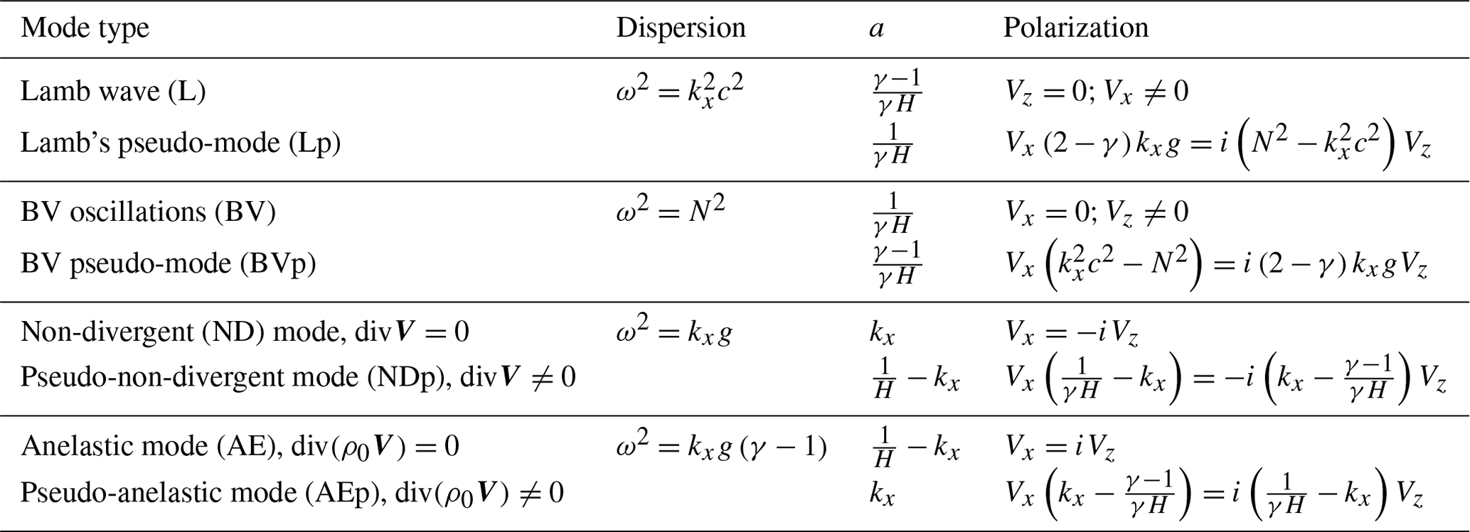
Thus, each evanescent mode can be associated with a pseudo-mode which satisfies the same dispersion relation but differs in polarization and dependence of the amplitude from the height, i.e., in its stratification. Table 1 presents the properties of different evanescent modes characteristic of the isothermal atmosphere: BV oscillations, Lamb waves, non-divergent and anelastic modes, along with associated pseudo-modes: BVp, Lp, NDp, AEp. Table 1 shows that for all pseudo-modes, the polarization changes depending on the value of k_x. Wave modes AE and ND at $k_x=\mathrm{1}/\mathrm{2}H$ completely coincide with AEp and NDp, respectively.

Table 1 Properties of different evanescent acoustic-gravity modes.

The location of the dispersion curves for anelastic and non-divergent modes relative to gravity and acoustic regions in the (ω,k_x) plane is shown in Fig. 1. The ${\mathit{\omega }}^{\mathrm{2}}=k_{x}g\left(\mathit{\gamma }-\mathrm{1}\right)$ mode touches the gravity region of freely propagating AGWs at the same value $k_x=\mathrm{1}/\mathrm{2}H$ at which the ω²=k_xg curve touches the acoustic region (see Fig. 1). In this case, the dispersion curves of AE and ND modes are symmetric relative to the “characteristic” curve (see Beer, 1974), which separates the AGW acoustic region from the AGW gravity region. In fact, the characteristic curve is the geometric mean of the dispersion curves of AE and ND modes with ${\mathit{\omega }}^{\mathrm{2}}=\sqrt{k_x^{\mathrm{2}}{g}^{\mathrm{2}}\left(\mathit{\gamma }-\mathrm{1}\right)}=N{k}_{x}c$.

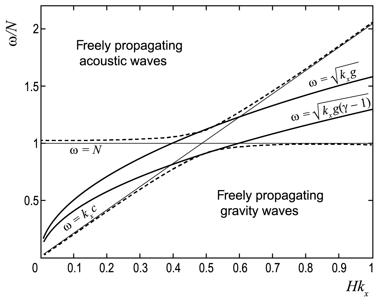
Figure 1 Dispersion dependencies ω=f(k_x): (1) boundaries between acoustic and gravity regions for freely propagating waves (dashed lines); (2) evanescent modes: $\mathit{\omega }=\sqrt{k_{x}g}$ (upper solid curve) and $\mathit{\omega }=\sqrt{k_{x}g\left(\mathit{\gamma }-\mathrm{1}\right)}$ (lower solid curve), ω=N (thin horizontal line), and ω=k_xc (thin sloping straight line).

From Fig. 1 we see that the dispersion curves of different evanescent modes have intersections at separate points. A Lamb dispersion curve with ${\mathit{\omega }}^{\mathrm{2}}=k_x^{\mathrm{2}}{c}^{\mathrm{2}}$ intersects the BV curve with ω²=N² at the point $k_x=N/c$. However, these modes cannot interact with each other by reason of different polarizations and values of a. At the same time, the pairs Lp-BV and L-BVp completely coincide in these properties and are indistinguishable at the intersection points.

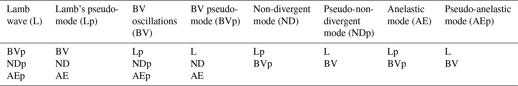
Dispersion curves ω²=k_xg and ${\mathit{\omega }}^{\mathrm{2}}=k_{x}g\left(\mathit{\gamma }-\mathrm{1}\right)$ intersect with the Lamb curve and the BV curve at points $k_x=\mathrm{1}/\mathit{\gamma }H$, $k_x=\left(\mathit{\gamma }-\mathrm{1}\right)/\mathit{\gamma }H$. In addition, the ND mode curve intersects with the Lamb curve at the same value k_x at which the AE mode curve intersects with the BV curve (see Fig. 1). ND and AE modes cannot interact with the Lamb mode and BV oscillations due to different polarizations (Table 1). Pseudo-modes NDp and AEp, at the points of intersection with the Lamb wave and the BV oscillations, have the same polarization and values of a. Similarly, ND and AE are indistinguishable at the points of intersection with Lp and BVp. Table 2 shows all evanescent modes that coincide with each other at the points of intersection of the dispersion curves, and between which interaction is possible. The cases of ND and AE mode curves intersection with curves ($a=\mathrm{1}/\mathrm{2}H)$, which separate the area of freely propagating AGWs from the evanescent area, are not presented in Table 2.

Table 2 The coincidence of the evanescent mode properties at the intersection points of the dispersion curves. Note: the bottom rows show the modes that are indistinguishable from the corresponding mode of the top row at the point of intersection of the dispersion curves.

3.1 The energy of evanescent modes in an isothermal atmosphere

In Sects. 2 and 3, we considered a model of an unbounded isothermal stratified atmosphere to determine which types of evanescent modes can satisfy the initial system of Eqs. (1) and (2). However, in an infinitely extended medium, the necessary condition for the existence of evanescent modes is the absence of unlimited growth of oscillation energy above and below the height level at which they are generated. It is easy to verify that in an isothermal infinite atmosphere, none of the modes listed in Table 1 satisfy this condition.

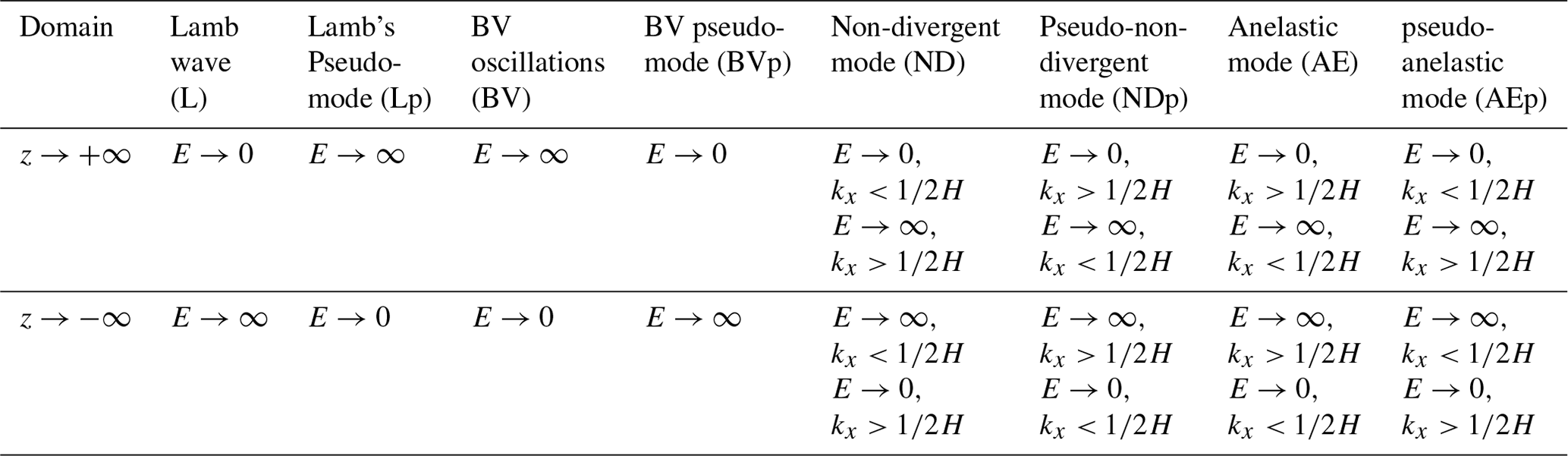
Suppose further that an evanescent wave is generated at a certain altitude level z=0. The kinetic energy density $E\sim \mathit{\rho }\left(z\right)\left(V_x^{\mathrm{2}}+V_z^{\mathrm{2}}\right)$ of waves should decrease both up and down from the level z=0. When $z\to +\mathrm{\infty }$ the energy density $E\sim \exp \left(\mathrm{2}a-\frac{\mathrm{1}}{H}\right)z\to \mathrm{0}$, if $a<\mathrm{1}/\mathrm{2}H$, and E→∞, if $a>\mathrm{1}/\mathrm{2}H$. When $z\to -\mathrm{\infty }$ the energy density E→0, if $a>\mathrm{1}/\mathrm{2}H$, and E→∞, if $a<\mathrm{1}/\mathrm{2}H$. Based on these considerations, it is not difficult to understand how the energy density varies with height for different types of evanescent modes in an infinite isothermal atmosphere (see Table 3). Therefore, for the realization of such modes, it is necessary to have boundaries in the medium at which the condition for reducing energy in both directions from this boundary can be satisfied.

Table 3 The change in energy density of evanescent modes with height in an infinite isothermal atmosphere.

The presence of boundaries is not the only condition that can limit the energy of the evanescent mode. If the equality $a=\mathrm{1}/\mathrm{2}H$ holds for these modes, then their energy does not vary with height in an isothermal atmosphere. For an infinite atmosphere, this solution does not seem to be physical, but it can make sense for a real atmosphere of finite height. As follows from Eq. (11), for the ND and AE modes, as well as their pseudo-modes, the condition $a=\mathrm{1}/\mathrm{2}H$ performed at the point $k_x=\mathrm{1}/\mathrm{2}H$. Also, at this point, the ND mode is identical to the NDp mode, and the AE mode completely coincides with AEp. In addition, when $k_x=\mathrm{1}/\mathrm{2}H$ these evanescent modes adjoin the border of regions of freely propagating AGWs (see Fig. 1).

Consider some features of the energy balance for the evanescent modes. It follows from Eq. (20) that

$$\begin{array}{}\text{(24)}& {\left|V_z\right|}^{\mathrm{2}}{\left(a-{\displaystyle \frac{g}{c^{\mathrm{2}}}}\right)}^{\mathrm{2}}=k_x^{\mathrm{2}}{\left|V_x\right|}^{\mathrm{2}}{\left(\mathrm{1}-{\displaystyle \frac{{\mathit{\omega }}^{\mathrm{2}}}{k_x^{\mathrm{2}}{c}^{\mathrm{2}}}}\right)}^{\mathrm{2}}.\end{array}$$

Combining Eqs. (22) and (24) gives the relation

$$\begin{array}{ll}{\displaystyle }& {\displaystyle }{\mathit{\rho }}_{\mathrm{0}}{\left|V_x\right|}^{\mathrm{2}}\left(\mathrm{1}-{\displaystyle \frac{{\mathit{\omega }}^{\mathrm{2}}}{k_x^{\mathrm{2}}{c}^{\mathrm{2}}}}\right)\left(a-{\displaystyle \frac{N^{\mathrm{2}}}{g}}\right)\\ \text{(25)}& {\displaystyle }& {\displaystyle }={\mathit{\rho }}_{\mathrm{0}}{\left|V_z\right|}^{\mathrm{2}}\left({\displaystyle \frac{N^{\mathrm{2}}}{{\mathit{\omega }}^{\mathrm{2}}}}-\mathrm{1}\right)\left({\displaystyle \frac{g}{c^{\mathrm{2}}}}-a\right).\end{array}$$

The average density of the kinetic energy of the perturbations is $E_{\mathrm{k}}=\frac{\mathrm{1}}{\mathrm{4}}{\mathit{\rho }}_{\mathrm{0}}\left(V_x^{\mathrm{2}}+V_z^{\mathrm{2}}\right)$, and of the potential energy it is $E_{\mathrm{p}}=\frac{\mathrm{1}}{\mathrm{4}}{\mathit{\rho }}_{\mathrm{0}}\left(V_x^{\mathrm{2}}\frac{{\mathit{\omega }}^{\mathrm{2}}}{k_x^{\mathrm{2}}{c}^{\mathrm{2}}}+V_z^{\mathrm{2}}\frac{N^{\mathrm{2}}}{{\mathit{\omega }}^{\mathrm{2}}}\right)$ (Yeh and Liu, 1974; Fedorenko, 2010). Therefore, from Eq. (25) it follows that for the evanescent modes E_k≠E_p. At the same time, for freely propagating AGWs, the equality E_k=E_p is always fulfilled (Yeh and Liu, 1974). At the point $a=\mathrm{1}/\mathrm{2}H$ where evanescent modes on the plane (ω,k_x) in Fig. 1 are adjacent to areas of freely propagating AGWs, the equality $a-\frac{N^{\mathrm{2}}}{g}=\frac{g}{c^{\mathrm{2}}}-a$ holds. Taking this circumstance into account, from Eq. (25) we obtain

$$\begin{array}{}\text{(26)}& {\displaystyle \frac{{\mathit{\rho }}_{\mathrm{0}}}{\mathrm{4}}}\left({\left|V_x\right|}^{\mathrm{2}}+{\left|V_z\right|}^{\mathrm{2}}\right)={\displaystyle \frac{{\mathit{\rho }}_{\mathrm{0}}}{\mathrm{4}}}\left({\left|V_x\right|}^{\mathrm{2}}{\displaystyle \frac{{\mathit{\omega }}^{\mathrm{2}}}{k_x^{\mathrm{2}}{c}^{\mathrm{2}}}}+{\left|V_z\right|}^{\mathrm{2}}{\displaystyle \frac{N^{\mathrm{2}}}{{\mathit{\omega }}^{\mathrm{2}}}}\right);\end{array}$$

that is, at this point E_k=E_p.

4 Evanescent modes at the interface of isothermal media

Let us consider the possibility of realization of evanescent modes in the atmosphere at a thin interface between two isothermal half-spaces of infinite extent, which differ in temperature T. Let the boundary be localized at some altitude level z=0. In the lower half-space (z<0) we have T=T₁, while in the upper half-space (z>0) we have T=T₂ and it is assumed that T₂>T₁. Note that a similar model was considered by Rosental and Gough (1994). We will search for solutions to Eqs. (1) and (2) in the form of $V_x,V_z\sim \exp \left(a_{\mathrm{1}}z\right)\exp \left[i\left(\mathit{\omega }t-k_{x}x\right)\right]$ for the lower half-plane and in the form $V_x,V_z\sim \exp \left(a_{\mathrm{2}}z\right)\exp \left[i\left(\mathit{\omega }t-k_{x}x\right)\right]$ for the upper half-plane. Substituting these dependencies into Eqs. (1) and (2) yields

$$\begin{array}{}\text{(27)}& {\displaystyle }& {\displaystyle }{a}_{\mathrm{1}}={\displaystyle \frac{\mathrm{1}}{\mathrm{2}{H}_{\mathrm{1}}}}\pm {\left({\displaystyle \frac{\mathrm{1}}{\mathrm{4}{H}_{\mathrm{1}}^{\mathrm{2}}}}-{\displaystyle \frac{{\mathit{\omega }}^{\mathrm{2}}}{c_{\mathrm{1}}^{\mathrm{2}}}}+k_x^{\mathrm{2}}-k_x^{\mathrm{2}}{\displaystyle \frac{N_{\mathrm{1}}^{\mathrm{2}}}{{\mathit{\omega }}^{\mathrm{2}}}}\right)}^{\mathrm{1}/\mathrm{2}},\text{(28)}& {\displaystyle }& {\displaystyle }{a}_{\mathrm{2}}={\displaystyle \frac{\mathrm{1}}{\mathrm{2}{H}_{\mathrm{2}}}}\pm {\left({\displaystyle \frac{\mathrm{1}}{\mathrm{4}{H}_{\mathrm{2}}^{\mathrm{2}}}}-{\displaystyle \frac{{\mathit{\omega }}^{\mathrm{2}}}{c_{\mathrm{2}}^{\mathrm{2}}}}+k_x^{\mathrm{2}}-k_x^{\mathrm{2}}{\displaystyle \frac{N_{\mathrm{2}}^{\mathrm{2}}}{{\mathit{\omega }}^{\mathrm{2}}}}\right)}^{\mathrm{1}/\mathrm{2}}.\end{array}$$

Here indices 1 and 2 denote the values in the lower and upper half-spaces, respectively.

The density of the kinetic energy of evanescent waves should decrease from the level z=0 both up and down. This condition limits the possible values of a₁ and a₂. In the upper half-space (z>0), when $z\to +\mathrm{\infty }$, the energy density $E_{\mathrm{2}}\sim \exp \left(\mathrm{2}{a}_{\mathrm{2}}-\frac{\mathrm{1}}{H_{\mathrm{2}}}\right)z\to \mathrm{0}$ if $a_{\mathrm{2}}<\mathrm{1}/\mathrm{2}{H}_{\mathrm{2}}$. In the lower half-space (z<0), when $z\to -\mathrm{\infty }$, the energy density $E_{\mathrm{1}}\sim \exp \left(\mathrm{2}{a}_{\mathrm{1}}-\frac{\mathrm{1}}{H_{\mathrm{1}}}\right)z\to \mathrm{0}$ if $a_{\mathrm{1}}>\mathrm{1}/\mathrm{2}{H}_{\mathrm{1}}$. Therefore, it is necessary to take in Eq. (27) for a₁ the solution with a “+” sign and in Eq. (28) for a₂ with a “−” sign, so that the energy decreases on both sides of the interface.

It is also necessary to consider that the possible values of a₁ and a₂ must satisfy the boundary condition (Tolstoy, 1963; Rosental and Gough, 1994), arising from Eqs. (1) and (2):

$$\begin{array}{}\text{(29)}& {\left.{\mathit{\rho }}_{\mathrm{1}}{c}_{\mathrm{1}}^{\mathrm{2}}{\displaystyle \frac{g{k}_x^{\mathrm{2}}-{\mathit{\omega }}^{\mathrm{2}}{a}_{\mathrm{1}}}{{\mathit{\omega }}^{\mathrm{2}}-c_{\mathrm{1}}^{\mathrm{2}}{k}_x^{\mathrm{2}}}}\right|}_{z=-\mathrm{0}}={\left.{\mathit{\rho }}_{\mathrm{2}}{c}_{\mathrm{2}}^{\mathrm{2}}{\displaystyle \frac{g{k}_x^{\mathrm{2}}-{\mathit{\omega }}^{\mathrm{2}}{a}_{\mathrm{2}}}{{\mathit{\omega }}^{\mathrm{2}}-c_{\mathrm{2}}^{\mathrm{2}}{k}_x^{\mathrm{2}}}}\right|}_{z=+\mathrm{0}},\end{array}$$

where ρ₁ and ρ₂ are the densities on both sides of the boundary. The procedure for deriving equality (Eq. 29) is exactly the same as in the papers by Cheremnykh et al. (2018a, b). When obtaining Eq. (29) we require continuity of the vertical velocity component (kinematic condition) and perturbed pressure (dynamic condition). In the barometric atmosphere we have ρc²=γp₀, where p₀ is the equilibrium pressure, which must be continuous across the interface. Therefore, when γ₁=γ₂, Eq. (29) can be written as

$$\begin{array}{}\text{(30)}& {\displaystyle \frac{g{k}_x^{\mathrm{2}}-{\mathit{\omega }}^{\mathrm{2}}{a}_{\mathrm{1}}}{{\mathit{\omega }}^{\mathrm{2}}-c_{\mathrm{1}}^{\mathrm{2}}{k}_x^{\mathrm{2}}}}={\displaystyle \frac{g{k}_x^{\mathrm{2}}-{\mathit{\omega }}^{\mathrm{2}}{a}_{\mathrm{2}}}{{\mathit{\omega }}^{\mathrm{2}}-c_{\mathrm{2}}^{\mathrm{2}}{k}_x^{\mathrm{2}}}}.\end{array}$$

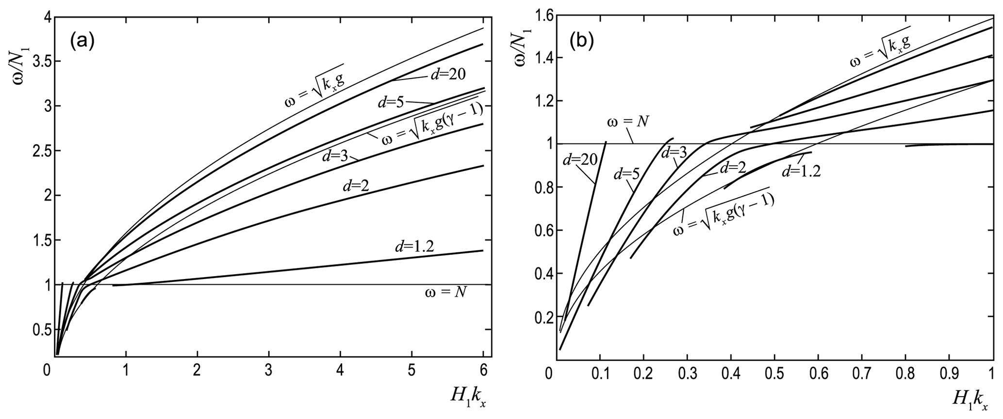
Figure 2 Dispersion dependencies ω=f(k_x) at the boundary of the discontinuity for different values of the parameter d. General dependence (a), long-wave part in more detail (b).

Dispersion dependencies of ω=f(k_x) calculated numerically by means of Eq. (30) are shown in Fig. 2a for different values of the parameter $d=H_{\mathrm{2}}/H_{\mathrm{1}}$. On each of these curves, the condition for decreasing energy up and down from the interface is satisfied. The long-wavelength part of the spectrum, where the most interesting features appear, is shown in more detail in Fig. 2b. Also shown in these figures are the dispersion curves $\mathit{\omega }=\sqrt{k_{x}g}$ and $\mathit{\omega }=\sqrt{k_{x}g\left(\mathit{\gamma }-\mathrm{1}\right)}$ for the ND and AE wave modes. The discontinuities of the ω=f(k_x) curves, as well as their cut-off for smaller k_x values, are due to requirements $a_{\mathrm{1}}>\mathrm{1}/\mathrm{2}{H}_{\mathrm{1}}$ and $a_{\mathrm{2}}<\mathrm{1}/\mathrm{2}{H}_{\mathrm{2}}$. Some features of the behavior of ω=f(k_x) will be discussed below.

As shown by Miles and Roberts (1992), the dispersion Eq. (30) can be rewritten to a polynomial form suitable for analysis:

$$\begin{array}{ll}{\displaystyle }& {\displaystyle }{\mathit{\omega }}^{\mathrm{8}}-\mathrm{2}{c}_{\mathrm{1}}^{\mathrm{2}}\left(d+\mathrm{1}\right)k_x^{\mathrm{2}}{\mathit{\omega }}^{\mathrm{6}}+\left[c_{\mathrm{1}}^{\mathrm{4}}{\left(d+\mathrm{1}\right)}^{\mathrm{2}}{k}_x^{\mathrm{4}}+\left(\mathrm{2}\mathit{\gamma }-\mathrm{1}\right)k_x^{\mathrm{2}}{g}^{\mathrm{2}}\right]\\ \text{(31)}& {\displaystyle }& {\displaystyle }\times {\mathit{\omega }}^{\mathrm{4}}-\mathrm{2}\left(\mathit{\gamma }-\mathrm{1}\right)c_{\mathrm{1}}^{\mathrm{2}}\left(d+\mathrm{1}\right)k_x^{\mathrm{4}}{g}^{\mathrm{2}}{\mathit{\omega }}^{\mathrm{2}}-c_{\mathrm{1}}^{\mathrm{4}}{\left(d-\mathrm{1}\right)}^{\mathrm{2}}{k}_x^{\mathrm{6}}{g}^{\mathrm{2}}=\mathrm{0}.\end{array}$$

Non-physical solutions (Miles and Roberts, 1992) arising from quadratic expressions under the radicals were excluded from consideration while obtaining Eq. (31) (see Eqs. 27 and 28). Solutions of Eq. (31) can be analyzed by studying their asymptotic behavior.

If $k_x^{\mathrm{2}}{c}_{\mathrm{1}}^{\mathrm{2}}\gg {\mathit{\omega }}^{\mathrm{2}}$, then from Eq. (31), we get

$${\displaystyle }{\mathit{\omega }}^{\mathrm{4}}-{\displaystyle \frac{\mathrm{2}{N}_{\mathrm{1}}^{\mathrm{2}}}{d+\mathrm{1}}}{\mathit{\omega }}^{\mathrm{2}}-{\displaystyle \frac{{\left(d-\mathrm{1}\right)}^{\mathrm{2}}}{{\left(d+\mathrm{1}\right)}^{\mathrm{2}}}}{k}_x^{\mathrm{2}}{g}^{\mathrm{2}}\approx \mathrm{0}.$$

It follows from this expression that

$$\begin{array}{}\text{(32)}& {\mathit{\omega }}^{\mathrm{2}}={\displaystyle \frac{\mathrm{1}}{d+\mathrm{1}}}\left[N_{\mathrm{1}}^{\mathrm{2}}+\sqrt{N_{\mathrm{1}}^{\mathrm{4}}+{\left(d-\mathrm{1}\right)}^{\mathrm{2}}{k}_x^{\mathrm{2}}{g}^{\mathrm{2}}}\right].\end{array}$$

Equation (32) contains an interesting dependence of the frequency on the parameter d. In the limit d→∞, the dispersion ω²≈k_xg of the ND (NDp) mode, independent of the properties of both environments, follows from Eq. (32). With d→1 and using Eq. (32), we obtain the dispersion of the BV (BVp) mode with the parameters of the lower medium, that is, ${\mathit{\omega }}^{\mathrm{2}}\approx N_{\mathrm{1}}^{\mathrm{2}}$. The indicated asymptotic features are visible on the curves shown in Fig. 2 below.

In the long-wave limit, i.e., at k_x→0, from Eq. (31) it follows that

$${\displaystyle }\left(\mathrm{2}\mathit{\gamma }-\mathrm{1}\right){\mathit{\omega }}^{\mathrm{4}}-\mathrm{2}\left(\mathit{\gamma }-\mathrm{1}\right)c_{\mathrm{1}}^{\mathrm{2}}\left(d+\mathrm{1}\right)k_x^{\mathrm{2}}{\mathit{\omega }}^{\mathrm{2}}-c_{\mathrm{1}}^{\mathrm{4}}{\left(d-\mathrm{1}\right)}^{\mathrm{2}}{k}_x^{\mathrm{4}}\approx \mathrm{0}.$$

Hence we find that

$$\begin{array}{}\text{(33)}& {\displaystyle }{\mathit{\omega }}^{\mathrm{2}}={\displaystyle \frac{c_{\mathrm{1}}^{\mathrm{2}}{k}_x^{\mathrm{2}}}{\mathrm{2}\mathit{\gamma }-\mathrm{1}}}\left[\left(\mathit{\gamma }-\mathrm{1}\right)\left(d+\mathrm{1}\right)+\sqrt{{\mathit{\gamma }}^{\mathrm{2}}{\left(d+\mathrm{1}\right)}^{\mathrm{2}}-\mathrm{4}d\left(\mathrm{2}\mathit{\gamma }-\mathrm{1}\right)}\right].\end{array}$$

For the considered small k_x, for different values of d, from Eq. (33) we obtain the family of Lamb-type acoustic modes (see Fig. 2b). For large values of d, using Eq. (33), we obtain the expression ${\mathit{\omega }}^{\mathrm{2}}\approx c_{\mathrm{1}}^{\mathrm{2}}{k}_x^{\mathrm{2}}d=c_{\mathrm{2}}^{\mathrm{2}}{k}_x^{\mathrm{2}}$; i.e., the oscillation frequency is determined by the characteristics of the medium in the upper half-space.

The evanescent modes' frequencies lie on the (ω,  k_x) plane between the acoustic and gravity regions of freely propagating AGWs determined for upper and lower media separately (see Fig. 1). It is necessary to take into account when considering evanescent modes at the boundary of two isothermal media with different temperatures that the evanescent regions are different in the upper and lower half-planes. On the  (ω,   k_x) plane, these regions are shifted more relative to each other the more the value of d is. At the same time, the wave modes at the interface of the media should remain evanescent in both media, and their dispersions should be enclosed within the overlap region of two evanescent regions. The cut-off curves for evanescent regions in the media under consideration are obtained in the case of the null expressions under the radicals in Eqs. (27) and (28). Gaps on the ω=f(k_x) dispersion curves are due to the evanescent areas of the two media not matching (see Fig. 3).

Figure 3 Dispersion dependencies of the ω=f(k_x) type at the temperature discontinuity boundary for d=2 (a), d=3 (b), d=5 (c), and d=20 (d). The dashed curves represent the boundaries of the areas with free propagation of AGWs in the upper and lower half-spaces, respectively.

Note that the dispersion curves ω=f(k_x) for values d≤4 are mostly inside both evanescent regions (see Fig. 3a, b), except for the longest waves. When d≥4, the dispersion curve ω=f(k_x) breaks into two separate branches (see Fig. 3c, d). The long-wave branch is acoustic, and another branch with k_x≥0.4H₁ is surface gravity by its physical nature.

5 Characteristic scales of ND and AE evanescent modes on the discontinuity

In an unlimited isothermal medium, evanescent modes are separate “pure” solutions of hydrodynamic equations. At the interface between two isothermal media with different temperatures, dispersion of the evanescent modes has a combined character, comprising different types of “pure” modes, depending on the value of the parameter d and spectral properties ω   (k_x).

For some values of d, the curves of the dispersion Eq. (30) approach fairly closely the curves ω²=k_xg and ${\mathit{\omega }}^{\mathrm{2}}=k_{x}g\left(\mathit{\gamma }-\mathrm{1}\right)$, and also intersect them at different points. These intersection points correspond to the specific value of k_x at which the dispersions of the ND and AE modes are realized, in the model under consideration, in a “pure” form. Let us now examine these cases in more detail. For this purpose, we substitute the dispersion relations ω²=k_xg and ${\mathit{\omega }}^{\mathrm{2}}=k_{x}g\left(\mathit{\gamma }-\mathrm{1}\right)$ directly into Eqs. (27) and (28), and then into the boundary condition (Eq. 30).

As was shown in Sect. 2, for the dispersion relations ω²=k_xg and ${\mathit{\omega }}^{\mathrm{2}}=k_{x}g\left(\mathit{\gamma }-\mathrm{1}\right)$, the values of each of the parameters a₁ and a₂ are the same for both relations and are determined by Eq. (11). Consider the valid values of a₁ and a₂ for these dispersions with regard to the requirement of energy decay in both directions from the interface $a_{\mathrm{1}}>\mathrm{1}/\mathrm{2}{H}_{\mathrm{1}}$ and $a_{\mathrm{2}}<\mathrm{1}/\mathrm{2}{H}_{\mathrm{2}}$.

5.1 Dispersion of the form ω²=k_xg

For a dispersion of the form ω²=k_xg, we first analyze the stratification of the ND mode with a₁=k_x, a₂=k_x. In order for the energy of this mode to decay in both directions from the discontinuity, the following inequalities $\mathrm{1}/\mathrm{2}{H}_{\mathrm{1}}<k_x<\mathrm{1}/\mathrm{2}{H}_{\mathrm{2}}$ must be satisfied, i.e., H₁>H₂. Therefore, the ND mode can be realized at the discontinuity if the ambient temperature in the upper region is less and the density is greater than they are in the lower region. This situation corresponds to the unstable state of the atmosphere (see Roberts, 1991).

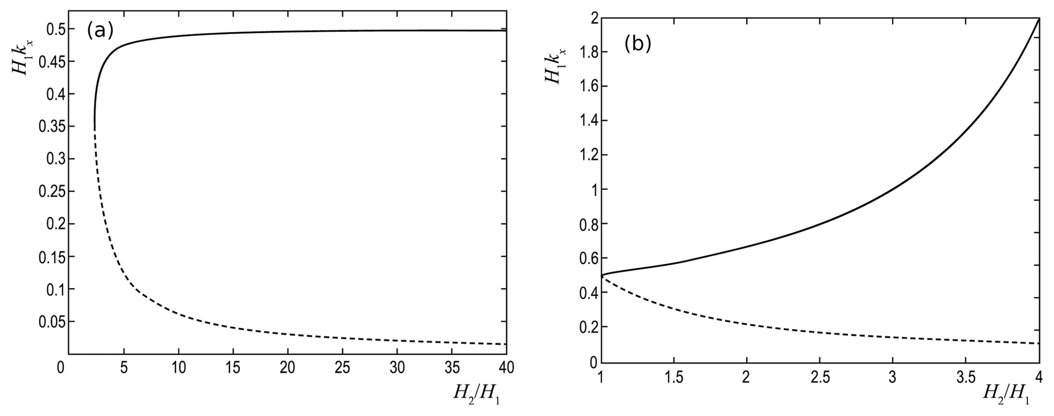
Figure 4 Horizontal scales k_xH₁, on which the modes with the dispersions ω²=k_xg (a) and ${\mathit{\omega }}^{\mathrm{2}}=k_{x}g\left(\mathit{\gamma }-\mathrm{1}\right)$ (b) are realized, depending on $d=H_{\mathrm{2}}/H_{\mathrm{1}}$. (See text for details.)

Take the stratification of the NDp modes in the form of $a_{\mathrm{1}}=\frac{\mathrm{1}}{H_{\mathrm{1}}}-k_x$, $a_{\mathrm{2}}=\frac{\mathrm{1}}{H_{\mathrm{2}}}-k_x$. The energy in this case decreases both ways from the discontinuity, if $\mathrm{1}/\mathrm{2}{H}_{\mathrm{2}}<k_x<\mathrm{1}/\mathrm{2}{H}_{\mathrm{1}}$, i.e., when H₂>H₁. This condition corresponds to the stable state and the case under consideration. For the NDp mode from the dispersion Eq. (30) we get

$$\begin{array}{ll}{\displaystyle }& {\displaystyle }{H}_{\mathrm{2}}\left({\displaystyle \frac{\mathrm{1}}{\mathit{\gamma }{H}_{\mathrm{2}}}}-k_x\right)\left(\mathrm{2}{k}_x-{\displaystyle \frac{\mathrm{1}}{H_{\mathrm{1}}}}\right)=\\ {\displaystyle }& {\displaystyle }{H}_{\mathrm{1}}\left({\displaystyle \frac{\mathrm{1}}{\mathit{\gamma }{H}_{\mathrm{1}}}}-k_x\right)\left(\mathrm{2}{k}_x-{\displaystyle \frac{\mathrm{1}}{H_{\mathrm{2}}}}\right),\\ \text{(34)}& {\displaystyle }& {\displaystyle }{k}_x\ne \mathrm{1}/\mathit{\gamma }{H}_{\mathrm{1}},k_x\ne \mathrm{1}/\mathit{\gamma }{H}_{\mathrm{2}}.\end{array}$$

From Eq. (34) it follows that

$$\begin{array}{}\text{(35)}& k_x={\displaystyle \frac{d+\mathrm{1}}{\mathrm{4}d{H}_{\mathrm{1}}}}\left(\mathrm{1}\pm \sqrt{\mathrm{1}-{\displaystyle \frac{\mathrm{8}d}{\mathit{\gamma }\left(d^{\mathrm{2}}-\mathrm{1}\right)}}}\right).\end{array}$$

Figure 4a shows values of k_x for which the dispersion curve ω²=k_xg intersects with the calculated dispersion curve ω=f(k_x) depending on the parameter d. The upper solid curve in this figure corresponds to the solution (Eq. 35) with the sign “+” before the radical and shows the points of intersection with the shorter wavelength branch. The lower dashed curve corresponds to the solution with a sign “−” and represents the points of intersection with the long-wavelength branch. For the upper curve $k_x\to \mathrm{1}/\mathrm{2}{H}_{\mathrm{1}}$ when d→∞. For d<2.5, there are no intersections of the curve ω=f(k_x) calculated numerically from Eq. (30) with the curve for the dispersion ω²=k_xg.

When combining the stratifications for ND modes as a₁=k_x and for NDp modes as $a_{\mathrm{2}}=\frac{\mathrm{1}}{H_{\mathrm{2}}}-k_x$, Eq. (30) yields the only possible value of $k_x=\mathrm{1}/\mathrm{2}{H}_{\mathrm{2}}$. For a combination of stratifications $a_{\mathrm{1}}=\frac{\mathrm{1}}{H_{\mathrm{1}}}-k_x$ (NDp), a₂=k_x (ND) we get $k_x=\mathrm{1}/\mathrm{2}{H}_{\mathrm{1}}$. Both of these cases do not satisfy the condition of energy decrease with height.

Thus, consideration of the possible values of a₁ and a₂ leads to the conclusion that on the interface of two isothermal media with H₂>H₁, the NDp mode can only be implemented with a dispersion ω²=k_xg and a specific scale $k_x\sim \mathrm{1}/\mathrm{2}{H}_{\mathrm{1}}$.

5.2 Dispersion of the form ${\mathit{\omega }}^{\mathrm{2}}=k_{x}g\left(\mathit{\gamma }-\mathrm{1}\right)$

For the AE stratification of the form $a_{\mathrm{1}}=\frac{\mathrm{1}}{H_{\mathrm{1}}}-k_x$, $a_{\mathrm{2}}=\frac{\mathrm{1}}{H_{\mathrm{2}}}-k_x$ and for the AEp stratification of the form a₁=k_x, a₂=k_x, from the dispersion Eq. (30) follows the identity H₁=H₂. Therefore, such modes are not realized at a temperature discontinuity. Apparently, to study the conditions of realization of AE and AEp modes, it is necessary to consider atmospheric models in which height profile H(z) is continuous.

It should be noted that for the dispersion of the form ${\mathit{\omega }}^{\mathrm{2}}=k_{x}g\left(\mathit{\gamma }-\mathrm{1}\right)$, cases of combined mode stratifications are possible, satisfying the condition of decreasing energy on both sides of the boundary. So, for the combination of stratifications a₁=k_x (AEp), $a_{\mathrm{2}}=\frac{\mathrm{1}}{H_{\mathrm{2}}}-k_x$ (AE) from Eq. (30), we obtain the relation

$${\displaystyle }{H}_{\mathrm{2}}{k}_x\left(\mathrm{2}-\mathit{\gamma }\right)=H_{\mathrm{1}}\mathit{\gamma }\left(k_x-{\displaystyle \frac{\mathit{\gamma }-\mathrm{1}}{\mathit{\gamma }{H}_{\mathrm{1}}}}\right),$$

whence $k_x=\frac{\mathit{\gamma }-\mathrm{1}}{H_{\mathrm{1}}\left[\mathit{\gamma }-\left(\mathrm{2}-\mathit{\gamma }\right)d\right]}$. In this case, the inequality $d<\mathit{\gamma }/\left(\mathrm{2}-\mathit{\gamma }\right)$ must be satisfied. When $\mathit{\gamma }=\mathrm{5}/\mathrm{3}$ we get the following restriction: d<5. Given this limitation and condition $k_x>\mathrm{1}/\mathrm{2}d{H}_{\mathrm{1}}$, we find that a mode with a dispersion of ${\mathit{\omega }}^{\mathrm{2}}=k_{x}g\left(\mathit{\gamma }-\mathrm{1}\right)$ and stratification of AE type for the upper half-space and of AEp type for the lower half-space can propagate at the boundary in the range $\mathrm{1}<d<\mathrm{5}$ and for $k_x>\mathrm{1}/\mathrm{2}{H}_{\mathrm{1}}$. For the stratifications $a_{\mathrm{1}}=\frac{\mathrm{1}}{H_{\mathrm{1}}}-k_x$ (AE), a₂=k_x (AEp) from Eq. (30) we obtain the relation

$${\displaystyle }{H}_{\mathrm{2}}\mathit{\gamma }\left(k_x-{\displaystyle \frac{\mathit{\gamma }-\mathrm{1}}{\mathit{\gamma }{H}_{\mathrm{2}}}}\right)=H_{\mathrm{1}}{k}_x\left(\mathrm{2}-\mathit{\gamma }\right).$$

It implies the ratio $k_x=\frac{\mathit{\gamma }-\mathrm{1}}{H_{\mathrm{1}}\left[\mathit{\gamma }d-\left(\mathrm{2}-\mathit{\gamma }\right)\right]}$, in which the parameter d can take any values with d>1, and the horizontal wave number is limited by the inequality $k_x<\mathrm{1}/\mathrm{2}{H}_{\mathrm{1}}$. Features of the behavior of the ${\mathit{\omega }}^{\mathrm{2}}=k_{x}g\left(\mathit{\gamma }-\mathrm{1}\right)$ mode at the discontinuity, depending on the scale k_x, are shown in Fig. 4b.

6 Discussion

Let us dwell on some of the results in terms of their use for the analysis of experimental data.

With the f-mode observed on the Sun, one should identify the mode that we classify as the ND mode, for which ω²=k_xg, V_z∼exp (k_xz) and divV=0 (Roberts, 1991). In the framework of the considered temperature discontinuity model, it was shown that with T₁<T₂ (corresponding to the chromosphere–corona interface) the condition for decreasing amplitude with height to both sides of the interface is satisfied only by the NDp mode with ω²=k_xg, $V_z\sim \exp \left(\frac{\mathrm{1}}{H}-k_x\right)z$ and divV≠0. When the ratio d→∞ (i.e., $H_{\mathrm{2}}/H_{\mathrm{1}}\to \mathrm{\infty })$, the NDp mode with $k_x\to \mathrm{1}/\mathrm{2}{H}_{\mathrm{1}}$ asymptotically approaches the ND mode. On the interface between the chromosphere and the solar corona, d is large but of finite magnitude: d∼50 (Jones, 1969; Athay, 1976). Therefore, the condition of the presence of a free surface, which is required for the realization of the ND mode, is fulfilled only approximately. Therefore, in the framework of the temperature discontinuity model, the f-mode observed on the Sun should not be associated with the non-divergent ND mode, but with non-divergent pseudo-mode NDp.

For the Earth's atmosphere, the maximum possible value of d is observed at the interface between the thermosphere with T₂∼800–1500 K (depending on solar activity) and the underlying atmosphere with T₁∼300 K. When d=5, the dispersion (Eq. 30) asymptotically tends to ${\mathit{\omega }}^{\mathrm{2}}=k_{x}g\left(\mathit{\gamma }-\mathrm{1}\right)$ with k_x→∞. Therefore, it can be expected that evanescent modes in this case will be close to ${\mathit{\omega }}^{\mathrm{2}}=k_{x}g\left(\mathit{\gamma }-\mathrm{1}\right)$.

In other layers of the Earth's atmosphere we have d≤1.3 (Jursa, 1985). As follows from Eq. (33), for small values of d≤1.3 and for the wavelengths in the interval $k_x\sim \left(\mathrm{0.5}-\mathrm{1.5}\right)H_{\mathrm{1}}$, the relation ω²→N² is satisfied (see Fig. 2). Therefore, it can be expected that at small positive temperature gradients in the atmosphere, waves with a frequency close to the frequency of Brent–Väisälä should prevail. These conclusions experimentally confirm (Shimkhada et al., 2009) the results of observations of short-period evanescent waves with small wavelengths at altitudes near the mesopause.

7 Main results

In the paper, different types of evanescent acoustic-gravity modes characteristic of an isothermal atmosphere are investigated. A new mode was derived in the form of anelastic acoustic-gravity wave mode with the dispersion equation ${\mathit{\omega }}^{\mathrm{2}}=k_{x}g\left(\mathit{\gamma }-\mathrm{1}\right)$. The main properties of the AE mode are presented in Table 1 in comparison with other known evanescent modes. It is shown that for both anelastic and non-divergent modes there are pseudo-modes that satisfy the same dispersions but have different polarization and the dependence of the amplitude of the disturbances on the height.

For AE and ND evanescent modes, the value of $k{}_x\to \mathrm{1}/\mathrm{2}H$ sets a special scale (wavelength) at which these modes are identical to their pseudo-modes AEp and NDp. In addition, at the same point they are adjacent to the boundaries of the continuous spectrum (AE mode to the gravity region and ND mode to the acoustic region, respectively).

The features of the evanescent modes' realization at the interface of two isothermal media are considered. It is shown that in this case, dispersions of evanescent modes are combined, merging the features of different types of modes characteristic of an unbounded isothermal atmosphere. This effect is most pronounced in the following asymptotic cases: (1) when d→∞, we obtain the dispersion for the ND (NDp) mode in the form ω²≈k_xg; (2) when d→1, for scales k_x∼H₁, a mode with ${\mathit{\omega }}^{\mathrm{2}}\approx N_{\mathrm{1}}^{\mathrm{2}}$ is realized; (3) for k_x→0, a Lamb wave with a dispersion relation of the form ${\mathit{\omega }}^{\mathrm{2}}\approx c_{\mathrm{2}}^{\mathrm{2}}{k}_x^{\mathrm{2}}$ is obtained, which depends only on the parameters of the medium in the upper half-space.

It was demonstrated that on the interface of two isothermal media with T₂>T₁, the NDp mode with the dispersion ω²=k_xg and the selected scale $k_x\sim \mathrm{1}/\mathrm{2}{H}_{\mathrm{1}}$ is realized. At the same time, the ND mode does not satisfy the condition of decreasing energy on each side of the interface. Dispersion ${\mathit{\omega }}^{\mathrm{2}}=k_{x}g\left(\mathit{\gamma }-\mathrm{1}\right)$ on the interface of two media is satisfied by the wave mode, which has different types of amplitude versus height dependencies at different horizontal scales k_x. When $k_x>\mathrm{1}/\mathrm{2}{H}_{\mathrm{1}}$, the height dependence of AE amplitude for z>0 and AEp amplitude for z<0 satisfy the condition of decreasing energy from the interface. By contrast, when $k_x<\mathrm{1}/\mathrm{2}{H}_{\mathrm{1}}$, this condition is satisfied by AEp amplitude for z>0 and AE amplitude for z<0.

It is important to note that according to our analysis in the framework of the temperature discontinuity model, (1) the f-mode observed on the Sun should not be associated with the non-divergent (ω²=k_xg, divV=0) mode, but with its non-divergent pseudo-mode (ω²=k_xg, divV≠0). (2) At the interface between the Earth's thermosphere and the underlying atmosphere it can be expected that evanescent modes with short wavelengths will be close to the new mode (${\mathit{\omega }}^{\mathrm{2}}=k_{x}g\left(\mathit{\gamma }-\mathrm{1}\right))$. (3) Oscillations with a frequency close to the frequency of Brent–Väisälä should prevail at altitudes near the Earth's mesopause.