Juice/SWI during the Lunar-Earth-Gravity-Assist (LEGA) – Part 3: Observations of the Earth as calibration target

On 19 and 20 August 2024 the Jupiter Icy Moons Explorer (Juice) executed during its cruise phase towards Jupiter a combined Lunar Earth Gravity Assist (LEGA) maneuver. These close flybys of the Moon and the Earth provided so far the best opportunity to test the behavior, performance, and calibration of the Submillimetre Wave Instrument (SWI) onboard Juice. This paper shows typical data taken during the Earth Gravity Assist and the following few days. Data quality and problems resulting from unexpected behavior of the hardware are discussed.

1 Introduction

The Submillimetre Wave Instrument (SWI) onboard Juice is a 29 cm single dish radio telescope operating simultaneously in the two frequency bands 530–638 and 1066–1286 GHz. Though the instrument's nominal functional and performance tests have been carried out already during the Near Earth Commissioning Phase (NECP) from May to July 2023, the combined Lunar Earth Gravity Assist (LEGA) provides a unique test environment to investigate in much more detail the performance and behavior of SWI in space. For the first time after the launch of Juice on 14 April 2023 the following kind of tests could be performed:

• The close distance of only about 6800 km to the Earth's surface during closest approach of the Earth Gravity Assist allowed to perform true limb sounding of the Earth's atmosphere. This observation geometry provides the largest spectral line contrast in brightness temperature during the entire cruise phase of Juice. It was necessary to check, if the instrument can measure and process such an input signal in the expected way.

• In addition this small distance between the Earth and the spacecraft allowed to observe the Earth as a target which fills the complete antenna pattern of the instrument – even a few days after closest approach the Earth had an apparent diameter of still ten to thirty times the full beam width of the instrument. This condition allows to check the total power calibration approach without detailed knowledge of the various telescope efficiency numbers (see e.g. Kutner and Ulich, 1981), first of all the telescope main beam efficiency, which is the ratio of power received in the main beam of the antenna pattern to the total power received by the antenna.

• The high brightness temperature level of the Earth's continuum radiation allowed a fast detection and evaluation of possible standing wave patterns created in the optical path of SWI's telescope.

• In general, the close distance and large apparent size of the Earth provided such a strong input signal to the instrument that spectral lines of water vapor, ozone, and oxygen could be detected within only a few seconds of integration time. This was not possible during NECP, because during that time the Earth's apparent diameter was only a fraction of SWI's beam width and the received signal was simply too weak. As a consequence the LEGA provided for the first time the opportunity to test the instrument's performance over the entire spectral tuning range.

• The huge amount of various optically thick and thin spectral transitions in the Earth's atmospheric spectrum, in combination with observations requiring only short integration times, provide a comprehensive data set to test and study the instrument's end-to-end measurement performance.

• The high spectral density and large number of closely spaced ozone spectral lines originating in the Earth's atmosphere allowed us to investigate and evaluate the behavior of the side band ratio for different tunings of the instrument.

• Finally scans across the sharp edge of the Earth's disk towards cold space provide data which allow an estimate of SWI's antenna pattern (Moreno et al., 2026, this issue). Especially the beam width of the pattern's main lobe could be measured with sufficient quality to verify the optical design of the telescope.

The basic idea of the analysis of SWI's LEGA data is to consider the Earth as a well-known target and to compare the observation results with theoretically expected results. Any deviation of the observations from the expectations is then considered primarily as an instrumental effect. However, this approach should not be taken as a strict rule: it is always possible that the Earth shows an unexpected behavior, which simply has not been taken into account in the modeling of the expected spectra. For example, currently we do not take into account small scale local atmospheric variations of clouds and tropospheric water vapor, which may be well resolved by the instrument at the extreme close distance to the Earth around the closest approach.

This paper is the third of a series of four publications in this special issue The first-ever lunar-Earth flyby: a unique test environment for Juice. Part 1 (Hartogh et al., 2026) provides a description of the functional characteristics of SWI and its operational principles; Part 2 (Cavalié et al., 2026) describes in detail the concept of SWI's observation modes, the operations planning, and the overall observation strategy of SWI for the Cruise Phase. This paper presents typical data obtained during LEGA and provides an overview of the current status of the ongoing data analysis to better understand the instrument behavior and related systematic measurement errors. Finally the last paper (Part 4, Moreno et al., 2026) of the series presents in-flight measurements of the instrument's main beam width, the beam side lobe level, the antenna pointing, and receiver co-alignment.

2 Instrument Description

In this section we shortly summarize the instrument and its measurement principle. SWI is essentially a small 29 cm single dish radio telescope. Using a polarizing grid as beam splitter behind the primary, secondary and tertiary mirrors of the telescope optics, the received electromagnetic radiation is fed into two independent heterodyne receivers, which are usually operated simultaneously. The two receivers are both tunable and operate in the frequency range of 530–638 and 1066–1286 GHz, respectively. Each of the two receivers is equipped with two different spectrometers: a chirp transform spectrometer (CTS) and a digital autocorrelation spectrometer (ACS). The CTS analyses the intermediate frequency signal in the range of 5.5–6.5 GHz with 10 000 equidistant channels (i.e. 1 GHz instantaneous bandwidth with 100 kHz resolution), while the ACS analyzes the intermediate frequency signal in the range of 4.4–8.8 GHz with 1024 equidistant channels (i.e. 4.4 GHz instantaneous bandwidth with 4.3 MHz resolution). At any time only one type of these two different spectrometers can be operated: either both receivers use the CTS or the ACS. Examples of spectra taken with these two kinds of spectrometers are shown in Sect. 4.3.

It is important to keep in mind that the receivers of SWI are so-called double sideband receivers, which are sensitive for two frequency bands at the same time: the upper sideband (USB) at frequencies given by the local oscillator frequency plus the intermediate frequency and the lower sideband (LSB) frequencies given by the local oscillator frequency minus the intermediate frequency. As a consequence two spectral line transitions with sky frequencies differing by e.g. 12 GHz will show up at the same intermediate frequency in the CTS spectrum. It is not possible to separate the two contributions from the two sidebands and then to show them separately as function of the sky frequency. Instead it is easier to always show the data as function of the intermediate frequency (IF) and to set up the theoretical models in a way to also provide double sideband data.

For more information see also Hartogh et al. (2026, this issue).

2.1 Total Power Calibration Approach

The challenge in spectro radiometric observations is the precise calibration of the received radiation intensity into physical units. A well-designed and properly built instrument always shows a linear relationship between the received radiation intensity (specified as Rayleigh-Jeans brightness temperature) and the observed IF-power.

To calibrate the received radiation intensity emitted by a science target – here the Earth – it is always necessary to observe two reference blackbody loads of known, different physical temperature – the hot load at temperature T_h and the cold load at temperature T_c. Observing these two loads provide two points (T_c,P_c) and (T_h,P_h), which allow to determine the two coefficients a and b of the linear calibration curve $P\left(T\right)=ax+b$ (see Fig. 1). Knowing the calibration curve then allows to calibrate any received power P_a in terms of the corresponding brightness temperature T_a:

$$\begin{array}{}\text{(1)}& T_{\mathrm{a}}={\displaystyle \frac{T_{\mathrm{h}}(P_{\mathrm{a}}-P_{\mathrm{c}})-T_{\mathrm{c}}(P_{\mathrm{a}}-P_{\mathrm{h}})}{P_{\mathrm{h}}-P_{\mathrm{c}}}}\end{array}$$

It is also possible to calculate the receiver noise temperature T_n, which corresponds to the observed power for a target at a temperature of zero Kelvin (i.e. which does not emit at all):

$$\begin{array}{}\text{(2)}& T_{\mathrm{n}}={\displaystyle \frac{T_{\mathrm{h}}{P}_{\mathrm{c}}-T_{\mathrm{c}}{P}_{\mathrm{h}}}{P_{\mathrm{h}}-P_{\mathrm{c}}}}\end{array}$$

SWI uses the cold sky as calibration cold load, which has a brightness temperature of essentially zero Kelvin at the observed frequencies. Entering T_c=0 into Eqs. (1) and (2) simplifies these equations to

$$\begin{array}{}\text{(3)}& T_{\mathrm{a}}={\displaystyle \frac{T_{\mathrm{h}}(P_{\mathrm{a}}-P_{\mathrm{c}})}{P_{\mathrm{h}}-P_{\mathrm{c}}}}\end{array}$$

and

$$\begin{array}{}\text{(4)}& T_{\mathrm{n}}={\displaystyle \frac{T_{\mathrm{h}}{P}_{\mathrm{c}}}{P_{\mathrm{h}}-P_{\mathrm{c}}}}\end{array}$$

If the instrument would be perfectly stable it would be sufficient to determine the calibration curve only once and then to calibrate any observed power P_a to the corresponding brightness temperature T_a. However, in practice the instrument is not stable: both the slope of the calibration curve and the noise temperature T_n do vary with time and environmental conditions. Especially temperature variations (e.g. caused by the instrument warm-up after power-on) cause a change of the amplification gain of various amplifiers within both the receiver and the spectrometer hardware, which translates directly into a change of the slope of the calibration curve. In addition temperature changes of the mixer diodes within the receiver hardware causes changes of the receiver noise temperature itself.

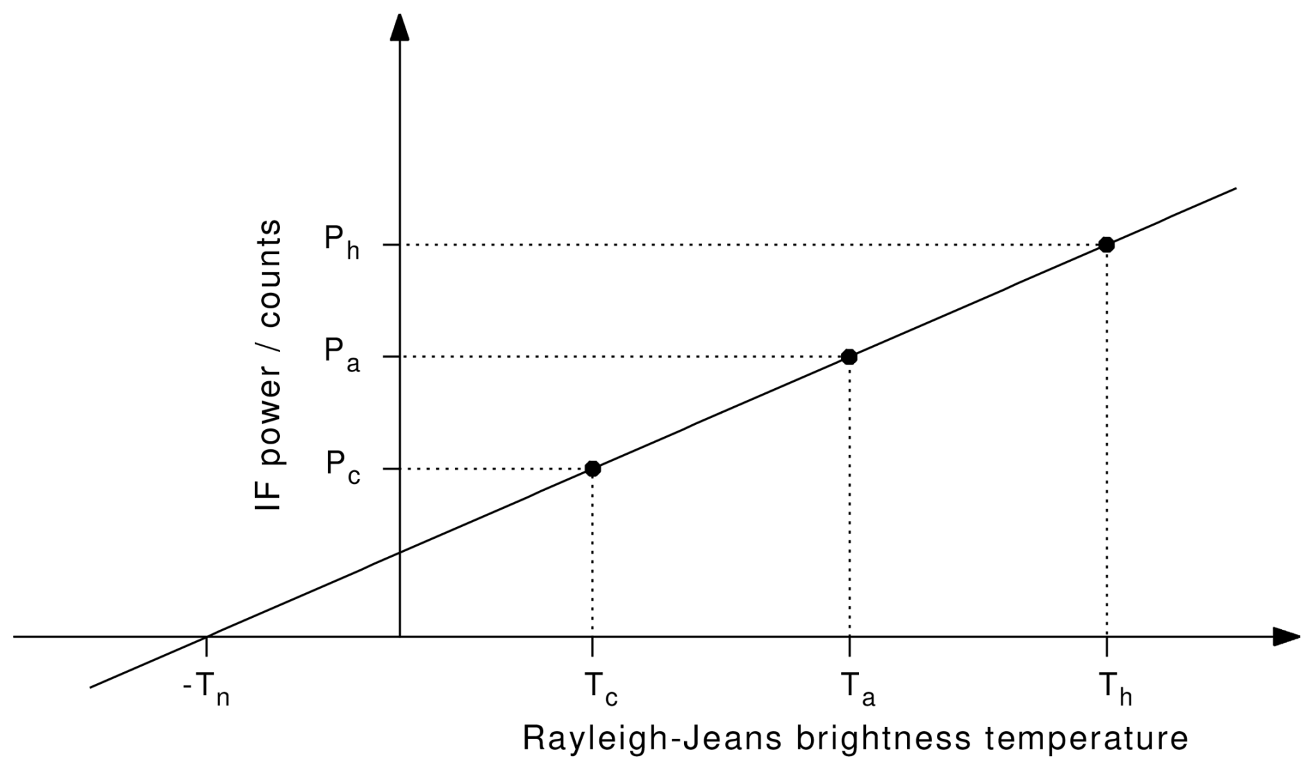
Figure 1 Illustrates the standard two-load total power calibration scheme using a hot and a cold load at different temperatures.

To compensate for such a variation it is necessary to periodically repeat the observations of the hot and cold load in order to obtain the correct calibration curve close to the time of any observation. The time interval between these periodic observations of the calibration loads depends solely on the stability and drift behavior of the instrument. It just has to be determined by observing the instrumental drift behavior under operational conditions (see e.g. Schieder and Kramer (2001) and Ossenkopf (2008) for a detailed discussion of this issue). As a rule of thumb usually this time interval between the periodic observations of the calibration loads is on the order of 10 to 30 s.

2.2 The Calibration Flip Mirror Issue

To properly perform the described calibration procedure SWI is equipped with an internal hot load and a so-called calibration flip mirror, which flips the receivers input signal from the telescope optics to the internal hot load (Hartogh et al., 2026, this issue). Unfortunately, after launch it has been discovered that the flip mirror mechanism has a significantly reduced lifetime: instead of the required minimum of 54 000 flip cycles the life time is currently estimated to about only 10 000 cycles before the mechanism finally gets mechanically stuck. This issue creates a serious problem for the intended usage of SWI. Therefore, the SWI team needs to find ways to reduce the amount of needed flip mirror cycles, and to find ways to perform the total power calibration without observing the internal hot load.

A possible way out of this situation has been provided by the empirical observation that the receiver noise temperature T_n is quite stable: repeating four times a measurement of T_n for a fixed set of 150 different tunings (75 tunings per receiver) shows a noise temperature depending on tuning, but for each tuning the individual measurements scatter only by about 4 % around the median value. This behavior of the instrument suggests to replace the hot load observation by the nearly stable receiver noise temperature. Combining Eqs. (3) and (4) allows to eliminate T_h and P_h:

$$\begin{array}{}\text{(5)}& {\displaystyle }{T}_{\mathrm{a}}& {\displaystyle }=T_{\mathrm{h}}{\displaystyle \frac{P_{\mathrm{a}}-P_{\mathrm{c}}}{P_{\mathrm{h}}-P_{\mathrm{c}}}}\text{(6)}& {\displaystyle }& {\displaystyle }=T_{\mathrm{h}}{\displaystyle \frac{P_{\mathrm{c}}}{P_{\mathrm{h}}-P_{\mathrm{c}}}}{\displaystyle \frac{P_{\mathrm{a}}-P_{\mathrm{c}}}{P_{\mathrm{c}}}}\text{(7)}& {\displaystyle }& {\displaystyle }=T_{\mathrm{n}}{\displaystyle \frac{P_{\mathrm{a}}-P_{\mathrm{c}}}{P_{\mathrm{c}}}}\end{array}$$

The expression $(P_{\mathrm{a}}-P_{\mathrm{c}})/P_{\mathrm{c}}$ allows to cancel out time variations of the slope of the calibration curve, as long as the time interval between the measurement of P_a and P_c is short enough. Performing Allan variance measurements under operational conditions helps to find the maximum length of this time interval (see e.g. Schieder and Kramer, 2001).

2.3 Observation Sequence

In practice this modified calibration approach means to execute any observation of a science target as a pair of observations: usually half of the total observing time is spent on the target while the other half is spent on cold sky. The SWI science observations are accomplished via different scripts or science modes that provide different ON/OFF calibration patterns (for a comprehensive summary see Cavalié et al., 2026, this issue). Depending on the stability of the instrument the total observing time needs to be split into many of such pairs with accordingly shortened observation time. In radio astronomy this approach is known as the so-called position switched observation sequence. An observation of the hot load is not done during the observation. Instead it is only necessary to have a trustworthy measurement of T_n, done at any time before or after the actual observation of the science target. Here the term trustworthy means to have a good idea how large the error of the used noise temperature is, i.e. how large the difference between the unknown noise temperature at the time of the science observation and the used noise temperature is. This knowledge can be only obtained by carefully and periodically monitoring the instrument behavior and its response to changing environmental temperatures – it is necessary to understand instrumental drift effects and take them properly into account.

3 Expected Spectra of the Earth

In order to evaluate the quality and measurement error of the SWI data it is necessary to have a model of the Earth capable to predict the expected data. The model consists of two parts: the first part is just the model of the Earth's atmosphere, i.e. the altitude profiles of temperature, pressure, and the mixing ratios of water vapor, oxygen, and ozone, to cover the main spectral features, and the second part is the radiative transfer model, which calculates the brightness temperature spectrum of the Earth as seen by SWI from space for the given atmospheric profiles.

3.1 Earth Atmosphere Model

The atmospheric temperature, pressure, water vapor and ozone mixing ratio profiles used in this work have been taken from the Modern-Era Retrospective Analysis for Research and Applications, Version 2 (MERRA-2) database (Gelaro et al., 2017; Global Modeling And Assimilation Office and Pawson, 2015). This database provides these data with a time resolution of three hours and a spatial resolution of 0.5° in latitude and 0.625° in longitude. Within the scope of the data analysis presented in this work we expect this database to reproduce the Earth's atmosphere with sufficient accuracy. Taking into account SWI's large footprint size (during the observations taken on e.g. the 21 August 2024 it had a diameter of 500 to 800 km for the 600 GHz receiver and about half this size for the 1200 GHz receiver), we decided to follow a climatological approach. Thus the data have been resampled the following way: average over 24 h in time, average over all longitudes (i.e. zonal average), and average over a 10° range in latitude (starting from the equator to 10°, 10 to 20°, 20 to 30°, …)

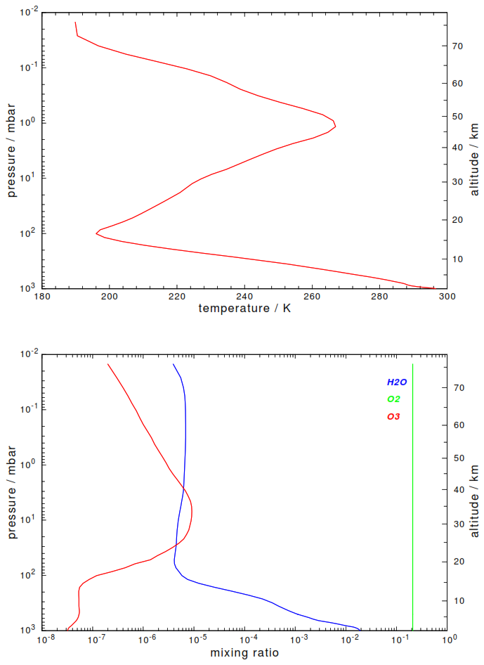
Figure 2 The temperature and mixing ratio profiles used in this work for the modeling of Earth spectra.

In this work we focus on the data analysis of SWI observations in nadir looking geometry. Because the sub-spacecraft latitude during the days after closest Earth approach has been varying between 16 and 17 degrees southern latitude, the Earth atmosphere model has been taken from the MERRA-2 data averaged between 10 and 20° southern latitude. Within the days when the LEGA Earth observations were performed, these averaged profiles do not show significant time variations with date, so the data for the 22 August 2023 (see Fig. 2) have been taken to represent the atmosphere for all Earth observations during the LEGA segment (20–23 August 2023).

3.2 Radiative Transfer Model

The radiative transfer model is a straight forward line-by-line and layer-by-layer model, which has been initially developed at MPS (Jarchow and Hartogh, 1995, 1997; Seele and Hartogh, 1999; Hartogh et al., 2010a, b; Rezac et al., 2014) and improved ever since. The atmosphere is represented by a stack of discrete layers of typically Δx_i=1 km thickness, where the temperature, pressure, and mixing ratios in each layer is uniform (see Fig. 3). The radiation I(x_N) passing through such a stack of N layers can be calculated as

$$\begin{array}{}\text{(8)}& \begin{array}{rl}{I}_N\equiv I\left(x_N\right)& =I\left(x_{\mathrm{0}}\right)e^{-{\sum }_{i=\mathrm{1}}^N{\mathit{\mu }}_i\mathrm{\Delta }{x}_i}\\ & +\sum _{i=\mathrm{1}}^N{J}_i{\mathit{\mu }}_i{e}^{-{\sum }_{j>i}^N{\mathit{\mu }}_j\mathrm{\Delta }{x}_j}\mathrm{\Delta }{x}_i\end{array}\end{array}$$

In case of a medium in thermodynamic equilibrium the source function J_i is given for each layer i by the Planck function

$$\begin{array}{}\text{(9)}& J_i(\mathit{\nu },T)={\displaystyle \frac{\mathrm{2}h{\mathit{\nu }}^{\mathrm{3}}}{c^{\mathrm{2}}}}{\displaystyle \frac{\mathrm{1}}{e^{h\mathit{\nu }/hT}-\mathrm{1}}}\end{array}$$

where T denotes the temperature and ν the frequency. Each layer's absorption coefficient μ_i is given by

$$\begin{array}{}\text{(10)}& {\mathit{\mu }}_i(\mathit{\nu },T)=N\cdot {\displaystyle \frac{\mathit{\nu }}{{\mathit{\nu }}_{\mathrm{0}}}}\cdot f(\mathit{\nu },{\mathit{\nu }}_{\mathrm{0}})\cdot I_{\mathrm{ab}}\left(T\right)\end{array}$$

where N is the number density of the emitting resp. absorbing molecules, ν₀ the transition frequency of the spectral line under consideration, and f(ν,ν₀) the spectral line shape function, which takes into account the pressure broadening effect caused by molecular collisions and the Doppler broadening effects caused by the thermal movement of the molecules. Here our radiative transfer code uses always the Voigt function, which is the convolution of a Lorentz function with a Gauss function. The Zeeman splitting of the oxygen transitions has not been taken into account in our radiative transfer model. As a consequence the model is currently not suitable to derive mesospheric temperatures from the oxygen transitions at 1120.7 and 1179.9 GHz, which both have been observed by SWI during LEGA. Finally the spectral line intensity I_ab(T) has been calculated using the HITRAN 2008 spectral line catalog (Rothman et al., 2009).

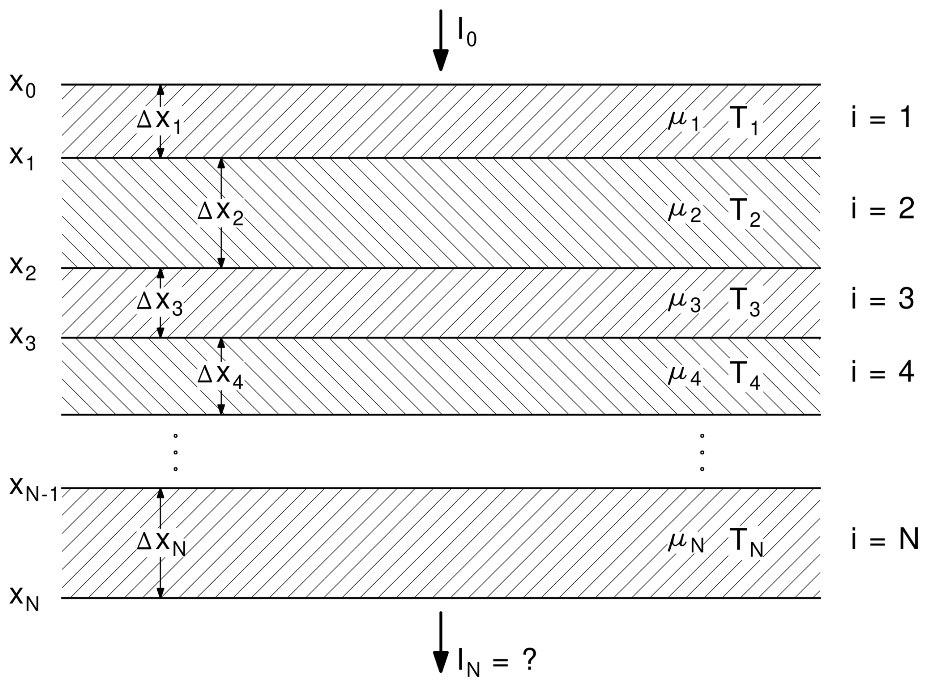
Figure 3 Illustration of the layer-by-layer approach used to calculate the radiation transfer through the Earth's atmosphere.

In case of several different molecular species and several spectral line transitions for each of these species the absorption coefficient needs to be calculated for each transition and each species separately and then these individual contributions finally need to be summed up to obtain the total absorption. Hence our model belongs to the line-by-line radiation transfer models.

4 Results

4.1 Total Power Calibration

The LEGA observations of the Earth offer the first opportunity to evaluate the SWI calibration approach as described in Sect. 2.1 and 2.2. The idea here is to focus on those observations when the instrument was pointing towards Earth's center, i.e. to analyze all observations with a nadir looking geometry. This approach has several advantages:

• Because of the close distance of the Earth during LEGA its apparent size is much larger than the beam width, so the Earth is essentially filling the entire beam. Thus no detailed knowledge of the beam pattern is needed, instead the expected spectra can be calculated using a simple pencil beam geometry for the radiative transfer.

• The data do not strongly depend on the exact pointing (contrary to e.g. limb viewing geometry). A miss-pointing on the order of a couple of beam-widths would not cause a significant change of the observed signal.

• No limb darkening or brightening effects need to be taken into account, because SWI sees only a small fraction of the apparent disk around its center.

Further simplification of the calculations is possible because the strong water vapor transitions within SWI's frequency range do not allow the ground emission to reach the instrument. For SWI the Earth simply looks like a gas planet with water vapor in the altitude range of 6 to 16 km providing the continuum background radiation. However, this situation does also provide some challenge: the continuum level depends critically on the exact temperature and water vapor concentration within this altitude range.

All of the observations executed during LEGA have been searched for nadir viewing spectra. These data have been found in 1- and 2-dimensional mapping observations (observation script name SWI_2D_MAP_OTF_V1) and spectral scans (observation script name SWI_SPECTRAL_SCAN_CTS_PS_V1 and SWI_SPECTRAL_SCAN_ACS_PS_V1). For a detailed description of these observation modes see Cavalié et al. (2026, this issue). In this work only observations involving the CTS are shown, the observations and analysis involving the ACS will be presented in a future publication.

4.1.1 1-Dimensional Maps

The observing scheme for 1- and 2-dimensional maps differs from the general principle described in Sect. 2.3. Instead of a set of target–sky pairs the target is observed on-the-fly, i.e. the target is rastered pixel by pixel without an intended observation of cold sky in-between (Ossenkopf, 2009). Instead cold sky data are automatically observed by simply setting the size of the map larger than the size of the target. An example of a 1-dimensional map is show in Fig. 4. It can be easily seen that the cold sky has been observed twice, once at the begin and a second time at the end of the observation. Averaging these spectra to a single P_c reference spectrum then allows to calculate the quantity $(P_{\mathrm{a}}-P_{\mathrm{c}})/P_{\mathrm{c}}$ for all of the pixels of the 1-dimensional scan. Multiplying all of these “partly” calibrated pixels with a single T_n spectrum obtained from a former or later measurement – which made use of the instrument internal hot load – then results in absolute scale calibrated data. Without explicitly mentioning a spectral channel index j in the equations it still needs to be understood that each pixel is associated with an entire CTS spectrum of 10 000 channels. Averaging these 10 000 channels to a single number for each individual pixel finally provides a simple overview of the observation versus time. Fig. 5 shows such kind of overview for the two spectrometers CTS1 and CTS2, respectively for the two receivers (CTS1 is connected to the 600 GHz receiver and CTS2 is connected to the 1200 GHz receiver). It can be clearly seen that the brightness temperature for the cold sky observing parts are close to zero and on the same level before and after crossing the Earth's disk. This indicates a stable instrument during the observation and justifies the on-the-fly approach a posteriori. To obtain now the spectrum in nadir viewing geometry only a small subset of the on-disk pixels around the central pixel have been averaged. During LEGA SWI has executed in total twelve such 1-dimension scans (either in vertical or horizontal direction), which could be analyzed this way.

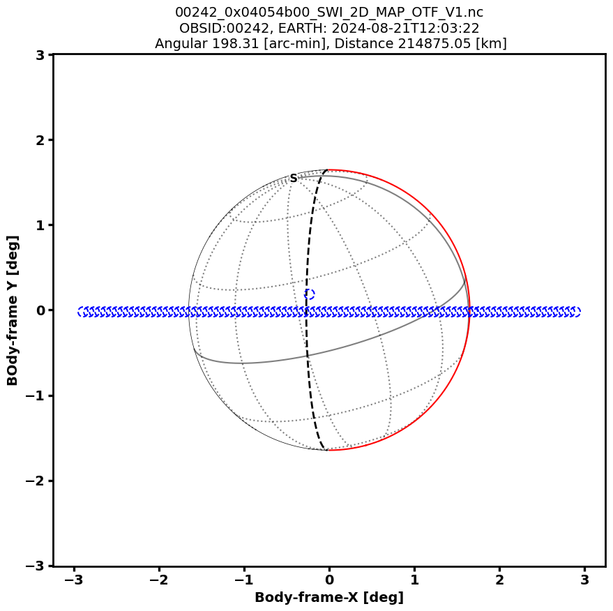
Figure 4 Example (ObsID 242) of the observing geometry for a 1-dimensional scan across the Earth's disk in East–West direction. The blue circles represent the position and beam size of the low frequency or so-called 600 GHz receiver. At the position of each circle an individual measurement or spectrum of 1.5 s integration time has been taken. The south pole is at the top of the disk (indicated by the “S”) and the equator is slightly below the center of the apparent disk.

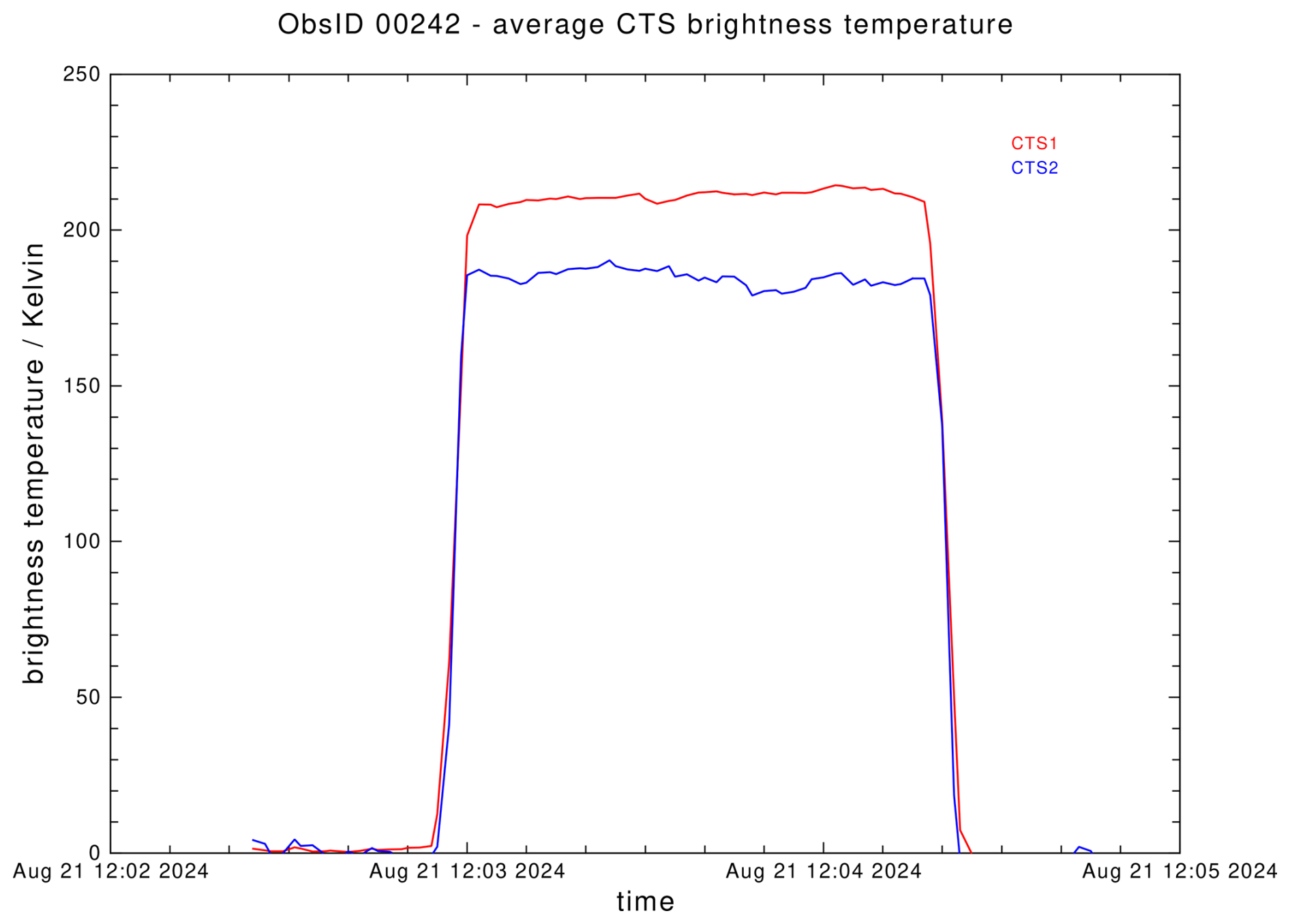
Figure 5 The average brightness temperature (average over the spectrometer channels) versus time for the observation shown in Fig. 4. Shown in red are the data obtained with the CTS1 connected to 600 GHz receiver, shown in blue are the data obtained with the CTS2 connected to 1200 GHz receiver. The whole scan across the Earth's disk took about 90 s.

4.1.2 2-Dimensional Maps

2-dimensional maps are just an extension of 1-dimensional maps. They are executed as a sequence of 1-dimensional scans where each scan is increasingly being shifted perpendicular to the scan direction. An example of such a 2-dimensional map with equal stepsize in x- and y-direction is shown in Figs. 6 and 7. To obtain the nadir viewing spectra only the central nine pixels of the apparent disk have been averaged to a single spectrum. This procedure guarantees to exclude limb contribution from the average. In total eight of such maps have been executed during LEGA, resulting in eight more nadir viewing data points.

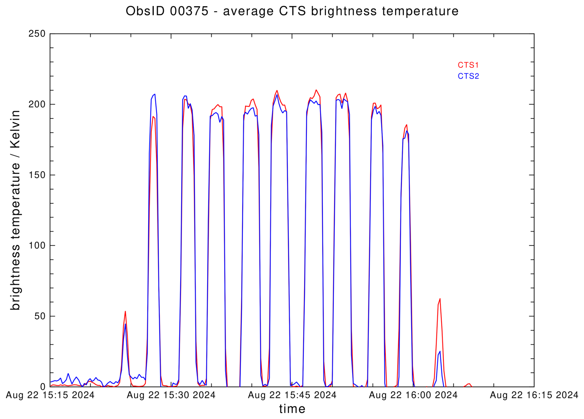
Figure 6 The average brightness temperature versus time for a 2-dimensional 15 × 15 pixel map of the Earth (ObsID 375). This figure is similar to Fig. 5, it can be considered just as a sequence of 1-dimensional scans. Each pixel had an integration time of 14 s, the entire map took nearly 1 h.

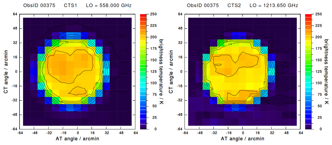
Figure 7 The average brightness temperature data shown in Fig. 6 plotted as function of the viewing direction. The data for the 600 GHz receiver are shown on the left, the data for the 1200 GHz receiver are shown on the right. The local oscillator frequency is indicated on top of each panel. The observed sky frequency is actually this local oscillator frequency plus 6 GHz (upper sideband) and minus 6 GHz (lower sideband). The orientation of the Earth is identical to Fig. 4, the south pole is at the top of the disk and the equator is slightly below the center of the apparent disk.

4.1.3 Spectral Scan Observations in Nadir Viewing Geometry

Spectral scan observations using the observation mode SWI_SPECTRAL_SCAN_CTS_PS_V1 (see Cavalié et al., 2026, this issue) are the third kind of observations with a clean nadir viewing geometry during LEGA. These observations are of special value because they cover a wide range of local oscillator tunings which are not covered by the 1- and 2-dimensional scans across the Earth. Here the observation scheme actually follows the scheme described in Sect. 2.3. Slightly simplified the basic building block of such observation is as follows:

1. let SWI view towards the center of the Earth

2. tune the local oscillator of the 600 and 1200 GHz receiver to the intended frequency

3. take simultaneously spectra with CTS1 and CTS2 (P_a data)

4. let SWI view towards cold sky

5. take simultaneously spectra with CTS1 and CTS2 (P_c data)

This building block is repeated until the list of intended tunings has been completely processed. In total seven observations with 11 tunings each have been executed during LEGA (see Cavalié et al., 2026, this issue), providing almost 77 further data points for the investigation of the quality of the total power calibration.

4.1.4 Comparison with the Earth Model

As previously discussed, in order to save the number of available flip cycles for the Jupiter science phase, nearly all of the data taken during LEGA do not include an observation of the instrument internal hot load. As described in Sect. 2.2, the current idea to still calibrate the data into physical units (i.e. Rayleigh-Jeans brightness temperature in Kelvin) is to take the needed noise temperatures T_n from instrument tests performed at other dates. Here we take advantage of the data collected during regular Payload Checkout Windows with measurements of system noise temperatures for a fixed set of 75 tunings for each of the two receivers. This receiver health test has been executed during the Near Earth Commissioning Phase in June 2023, during the first and second Payload Checkout in January respectively July 2024, and finally a fourth time during Payload Checkout Window 3 in March 2025. So as best estimate for the (not measured) noise temperatures during LEGA the median value for each tuning has been taken. It has been observed empirically that almost all of the noise temperature measurements scatter within just 4 % around the corresponding median value. This observation is valid for both the 600 GHz and the 1200 GHz receiver. Because T_n in Eq. (7) acts as a scaling factor for T_a the immediate conclusion is that the error of the calculated T_a cannot be smaller than 4 % of its value. This means a finally calibrated brightness temperature of e.g. 200 K is expected to have an error of 0.04 × 200 K = 8 K. This value defines the task of the comparison with the expected brightness temperature of the Earth Model: do the calibrated data of the LEGA observations fall within a range of ±8 K around the expected values? This comparison also answers the question of whether the measured system noise temperatures are reasonable at all, or if they are systematically off.

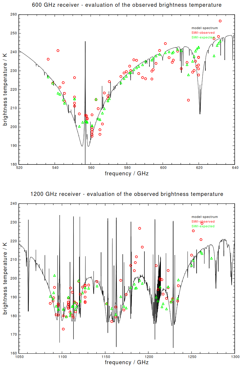
Figure 8 Comparison of the calibrated brightness temperatures (red circles) for the 600 GHz receiver with the expected brightness temperatures (green triangles) from the model of the Earth. Shown as black solid curve is the single sideband model spectrum of the Earth.

Figure 8 shows the results for the 600 GHz and the 1200 GHz receiver. The red circles show the calibrated brightness temperatures from the observations, the green triangles show the corresponding expected value from the model spectrum of the Earth. Shown as black solid curve is the single sideband model spectrum of the Earth. Because SWI is a double sideband receiver each observation has been plotted versus the corresponding LO-frequency – it must be kept in mind that each symbol represents the signal contribution from a frequency ±6 GHz apart from the LO frequency. In exactly the same way the expected brightness temperatures (green symbols) have been calculated from the underlying single sideband spectrum. Looking first at the comparison results for the 600 GHz receiver it is obvious that the LEGA data are consistent with the overall shape of the Earth's spectrum. With the exception of only a few outliers we found that 90 % of the calibrated brightness temperatures deviate less than 5 % from the expected value, which is close to the value expected from the scatter of the noise temperature measurements. However, the 1200 GHz receiver shows a slightly inconsistent pattern. Up to frequencies of 1170 GHz the deviation of the measured and expected brightness temperatures is well within the expected 4 % deviation, but around 1185 and 1260 GHz the observed brightness temperatures are found to be systematically about 5 % to 6 % too high. This inconsistent behavior cannot be explained by an inappropriate Earth model, because the data do match the expectations very well within the frequency range of 1080 to 1170 GHz. Instead it is considered to be an instrumental effect and needs more investigation of the SWI hardware behavior itself.

In summary two conclusions can be drawn from this comparison: (1) the noise temperatures measured during commissioning phase and the first three instrument checkouts are valid and accurate – there are outliers, but the data are not consistently off in a systematic way; (2) so far the calibrated data presented in this work do not suggest to introduce any instrument specific or hardware related correction factors, calibration load emissivities, or load coupling efficiencies. The straight forward calibration approach as described in Sect. 2.1 works already well, providing a robust and reliable calibration of the measured output power to the physical quantity of brightness temperature.

4.2 Limb Scan

The small distance of only 6800 km at the Earth's closest approach on 20 August 2024 at 21:57 UTC allowed a very special observation, which can be performed only within a small time window around that event: true limb scanning of the Earth's atmosphere. True limb scanning means that the beam width of the instrument at the tangential point along the viewing direction is much smaller than the thickness of the atmosphere itself. This observation geometry provides the longest path length through the atmosphere and thus the largest amplitude for any spectral line. It is an excellent test case to check within only a minute of observing time if SWI is measuring the correct spectral line shape or if there are any unexpected instrumental effects which severely distort the observed spectra.

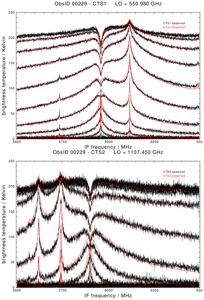
The observation scheme was identical to the case of 1-dimensional maps as described in Sect. 4.1.1: spectra have been taken on-the-fly without any periodic observations of cold sky in between. The viewing direction of SWI was an inertial pointing chosen to let the Earth drift under SWI's beam during the gravity assist maneuver. The local oscillator of the 600 and 1200 GHz receivers were tuned to 550.980 and 1107.450 GHz, respectively, which allowed to observe in the upper sideband the strong ground state transitions of water vapor at 557 GHz (ortho water) and 1113 GHz (para water). The Earth's limb entered SWI's field of view on 20 August 2024 at 21:20 UTC, 30 min before closest approach. At that time the altitude of the Juice spacecraft above ground was 12 020 km and the distance to the limb was 17250 km, resulting in a beam width at the limb of 40 and 23 km for the 600 GHz respectively the 1200 GHz receiver. SWI's beam went across the Earth's disk with a speed of 6.65 km s⁻¹, so the limb scan across the 100 km thick atmosphere took only 15 s. Because an individual spectrum has been taken every 1.625 s the nominal altitude stepsize between individual spectra is 10.8 km – less than the beam width of the instrument for both receivers. In other words the spectra – especially for the 600 GHz receiver – do heavily overlap regarding the sampled altitude range. Figure 9 shows in black the set of observed limb spectra for both the 600 GHz and the 1200 GHz receiver and in red the corresponding set of expected spectra. The 600 GHz receiver spectrum shows the 110–101 target transition of ortho-H${}_{\mathrm{2}}^{\mathrm{16}}$O at an IF frequency of 5950 MHz and two additional O₃ transitions at an IF frequency of 5730 resp. 6120 MHz. The 1200 GHz spectrum shows the 111–000 target transition of para H${}_{\mathrm{2}}^{\mathrm{16}}$O at an IF frequency of 5900 MHz (upper sideband), the 111–000 transition of para H${}_{\mathrm{2}}^{\mathrm{18}}$O at an IF frequency of 5750 MHz (lower sideband), and an O₃ transitions at an IF frequency of 5620 MHz.

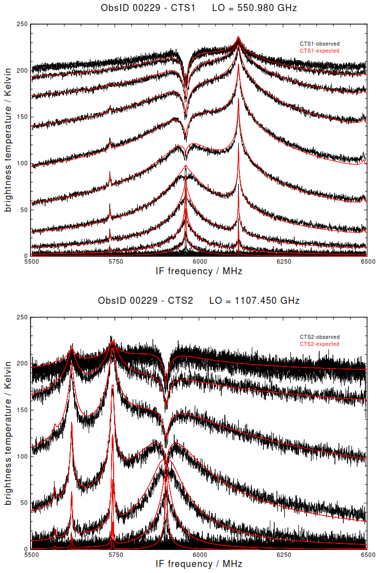
Figure 9 The set of limb spectra (ObsID 229, black curves) observed on 20 August 2024 at 21:20 UTC, 30 min before closest approach to the Earth. Each trace corresponds to a single spectrum taken with an integration time of 1.5 s. Because SWI's viewing direction slowly crosses the Earth's limb from space towards the center of the Earth during this observation, each spectrum has been taken at a different tangential height, which leads to an increasing pressure broadening for each individual spectral line. Shown in red are the expected spectra as calculated with the Earth model described in Sect. 3.

The agreement between the expected and observed spectra is excellent, especially the absence of any periodic baseline ripples caused by e.g. standing waves in the instrument optical path demonstrates a high quality of the SWI hardware.

4.3 Spectral Scan

The scientific purpose of a Spectral Scan observation is to explore the spectrum of a science target (Jupiter and the Galilean satellites) over the entire frequency range covered by SWI. This is done by systematically stepping the local oscillator frequency through the entire tuning range of both receivers and to take spectra either in position switching or frequency switching mode. The basic building block of such an observation in position switching mode has been already described in Sect. 4.1.3; for a detailed description of these observing modes see Cavalié et al. (2026, this issue).

During the LEGA a large amount of these spectral scan observations have been performed in order to test the implemented observation schemes (also called observation scripts) and also to obtain first information about the behavior and performance of the instrument when the local oscillator frequency is not stable anymore for hours, but changes literally every minute. To evaluate the instrument performance here the Earth signal is once again considered as basically known test signal and deviations from the expected spectra are taken as a strong indicator pointing to unexpected hardware behavior or improper use of the existing hardware. This way it was especially possible to evaluate the entire table of local oscillator settings: which tunings work well, which ones have to be taken with precaution, and which ones do fail and must be marked as unusable.

In the following sections two examples of such spectral scan observations are shown: the first observation made use of the CTS as spectrometer while the second observation used the ACS instead.

4.3.1 CTS

Figure 10 shows an example (ObsID 289 and 290) of a position switched spectral scan using the CTS as spectrometer. The pointing direction has been chosen towards the Earth's limb to increase the spectral line amplitude. The black curve shows the observed spectra and the red curve the expected spectra. Solid blue ticks indicate transitions of H${}_{\mathrm{2}}^{\mathrm{16}}$O, dotted blue ticks of H${}_{\mathrm{2}}^{\mathrm{17}}$O, dashed blue ticks of H${}_{\mathrm{2}}^{\mathrm{18}}$O, solid and dashed green ticks those of ¹⁶O₂ respectively ¹⁶O¹⁸O, and the red ticks finally indicate the vast majority of ¹⁶O₃ transitions. Contrary to the data shown before in this paper here the y-axis does not provide the brightness temperature in units of Kelvin, but instead provides the radiation intensity as a dimensionless number. The reason for this is as follows: most of the tunings executed during the LEGA spectral scan observations have been used for the very first time, but because of the calibration flip mirror issue described in Sect. 2.2, it has been decided not to take spectra of the internal hot load. Consequently we do not have T_n data for all of the tunings. Hence the data can be only partly processed to the quantity $(P_{\mathrm{a}}-P_{\mathrm{c}})/P_{\mathrm{c}}$. To enable easy comparison with the expected spectra then both – the observed and the expected spectrum – have been normalized to unity, i.e. the entire spectrum has been divided by its average: $y_{j,\mathrm{normalized}}=y_j/{\sum }_{j=\mathrm{1}}^m{y}_j$. This way to compare the observed data with the expected spectra has been also applied to the ACS data shown in Figure 11. Here it is not the intention to identify and explain each single detected transition, but instead to show the quality of the observed spectra for a set of well working tunings.

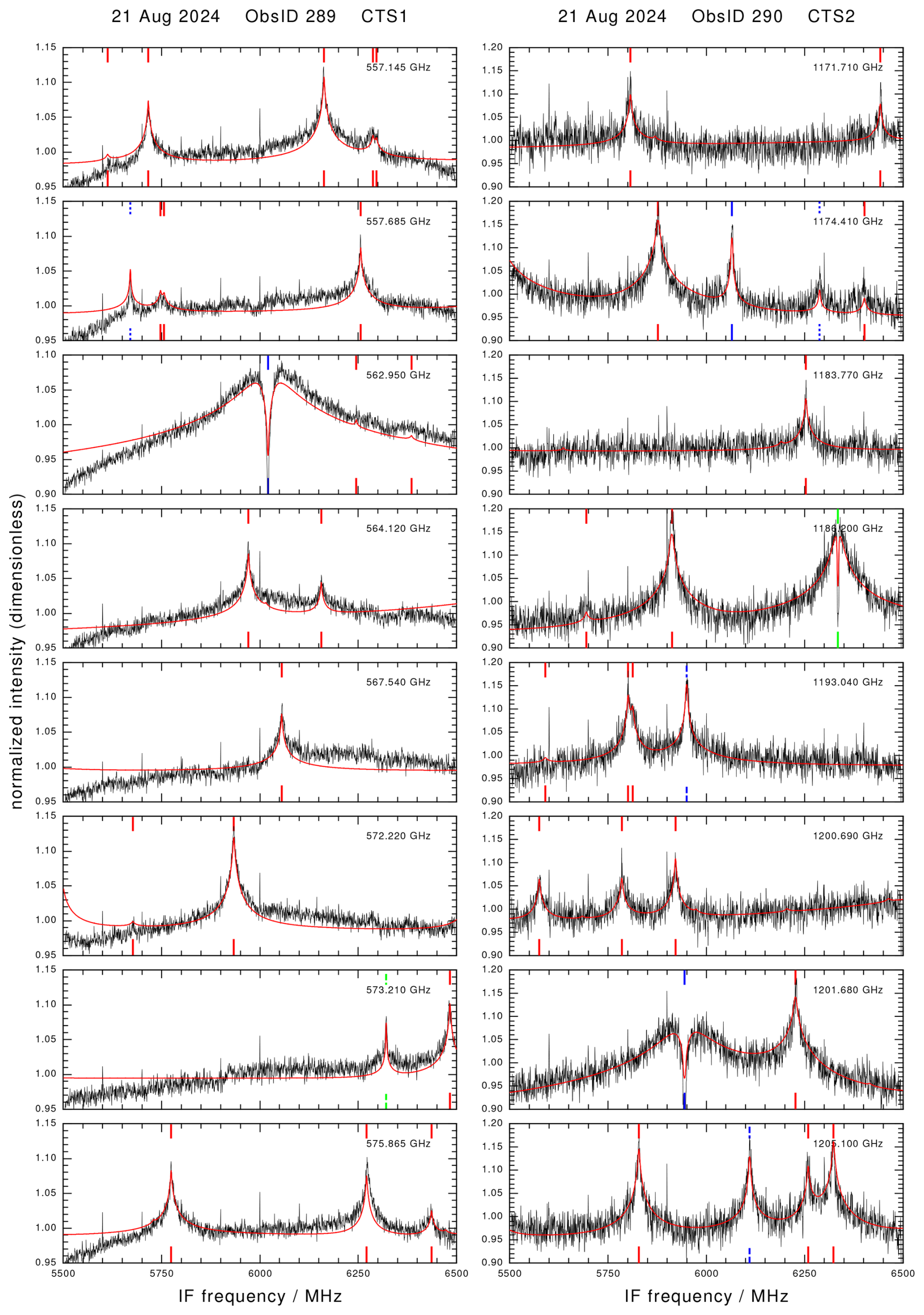
Figure 10 Example of a position switched spectral scan in limb viewing geometry using the CTS as spectrometer. The left column shows spectra obtained with the 600 GHz receiver, the right one those obtained with the 1200 GHz receiver. The local oscillator frequency of each single spectrum is indicated within each panel; the coloured ticks indicate the source molecule of each spectral line transitions and are explained in Sect. 4.3.1. The integration time for each individual spectrum was 25 s.

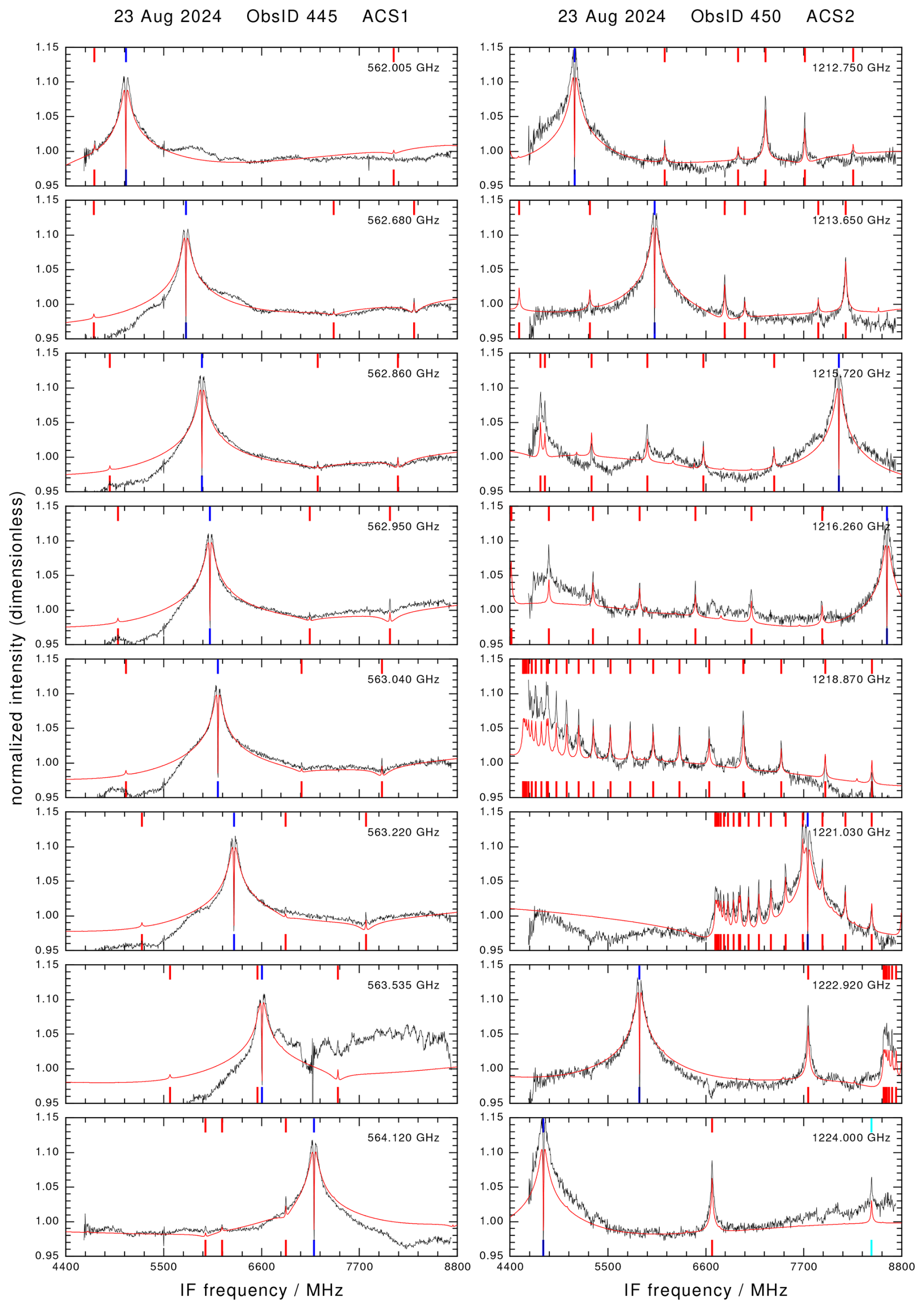
Figure 11 Example of a position switched spectral scan in nadir viewing geometry using the ACS as spectrometer. The left column shows spectra obtained with the 600 GHz receiver, the right one those obtained with the 1200 GHz receiver. The local oscillator frequency of each single spectrum is indicated within each panel; the coloured ticks indicate the detected molecule as in Fig. 10; the single light blue tick in the lower right panel indicate the J=1–0 transition of HF at 1232.476 GHz. The integration time for each individual spectrum was 10 s.

When looking carefully at the spectra a set of weak narrow peaks at IF frequencies of 5600, 5700, 5800, … MHz are visible. These peaks are actually an instrumental effect, because a frequency comb with 100 MHz fundamental frequency is used for the frequency calibration of the CTS spectra. This calibration signal is turned off before taking science data, but because of a too short delay between the turn off command and the start of the science observation there is still a remainder visible in the science data. Increasing that delay will be the proposed solution to avoid these remainders in future.

4.3.2 ACS

Figure 11 shows an example (ObsID 445 and 450) of a position switched spectral scan using the ACS as spectrometer. In this case the pointing direction has been chosen towards the Earth's nadir direction. This spectral scan demonstrates clearly, how advantageous it is to calculate the expected spectrum as double sideband spectrum, if the observed spectrum is a double sideband spectrum as well. The upper right panel for ACS2 with local oscillator frequency 1212.750 GHz shows at an IF frequency of 5080 MHz the strong 422–413 transition of para-H₂O in the lower sideband of the 1200 GHz receiver. Increasing stepwise the local oscillator lets this transition move to higher IF frequencies and finally leave the IF range analyzed by the ACS. Instead – when further increasing the LO frequency to 1218.870 GHz – a set of ozone transitions are observed in the lower sideband. Continuing to increase the LO frequency lets this ozone pattern move towards higher IF frequencies, but at the same time another strong transition enters the spectrometer's frequency range and is moving in the opposite direction from higher to lower IF frequencies. This transition is the strong 220–211 transition of para-H₂O, but now detected in the upper sideband of the receiver. This spectral transition is actually at a 14 GHz higher sky frequency than the set of ozone transitions, but overlaps with these ozone transitions in the IF. It is clearly visible that this effect is only properly modeled when modeling the expected spectrum also as a double sideband spectrum.

Now looking at all of the spectra for the ACS1 it is obvious that the spectrum for the local oscillator frequency of 563.535 GHz is different from all of the others: it does not match the expected spectrum as well as the other spectra do, though the change in LO frequency is only small. Exactly this is the way how we evaluate the instrument performing for each tuning: if the deviation from the expectation is significantly larger than on average, then that tuning must be flagged “bad” and not used any longer until a workaround is found. Without the Earth providing a known and strong test signal this efficient procedure would not have been possible.

5 Conclusions

In this paper we present first results of the Earth observations executed with the SWI instrument during the LEGA, which provided a unique opportunity to thoroughly investigate the instrument's performance using the Earth as a known calibration target. The following conclusions have been drawn from the work presented in this paper:

1. The system temperatures as measured in space are valid and can be directly used for the total power calibration of SWI's science data.

2. The system temperatures of both receivers appear to be sufficiently stable to allow a lookup table approach for the total power calibration, which mitigates the limited lifetime problem for the hot load calibration flip mirror. Though this approach works in general very well, there are many observations, which deviate by more than 7 % from the expected value. Especially the 1200 GHz receiver displays in the range of 1170 to 1220 GHz local oscillator frequency deviations of 8 % to 12 %. Taking into account the fact that the power consumption of the receivers change with the tuning, these large deviations may be caused by different thermal stabilization times of the receiver hardware. So more detailed investigation of the instrument's drift behavior have to be carried out first, to understand how to best mitigate these effects.

3. The spectra provided by SWI do not show strong and severe standing wave ripples, which are usually present in optical on-axis telescope designs – here SWI clearly benefits from its off-axis telescope design.

4. The instrument internal xy-scanning mechanism (the so-called AT- and CT-mechanism) works reliably: 2-dimensional maps of the Earth are reproducable and do not suffer from severe loss of motor steps.

This work covers just a fraction of the extensive data set of SWI LEGA observations; further work is needed e.g. to complete the total power calibration of the ACS data in order to obtain a comprehensive understanding of the instrument performance.