A near-sunset atmospheric sounding during the 14 October 2023 annular solar eclipse over Natal

Solar eclipses are transient atmospheric events that cause rapid localized reduction in solar radiation, which produces complex changes associated with the vertical coupling of the layers. This study investigates how the neutral atmosphere responded vertically to the 14 October 2023 annular solar eclipse over Natal, Brazil (5.79° S, 35.2° W). This event presented a unique setup i.e., the maximum obscuration of ∼ 88.5 % occurred near sunset in a coastal transition between land and ocean. A stratospheric balloon sounding launched immediately before the umbra reached Natal was used. The balloon collected atmospheric profiles (temperature, pressure, relative humidity, and ozone concentration) over 1.45 h, with the umbra passing over the balloon at ∼ 22.35 km altitude for 3 min and 36 s. Comparison with average October profiles, model and reanalysis data revealed clear vertical patterns: (i) A notable cooling of 4–5 K in the tropopause region (14 km altitude); (ii) increased vertical temperature fluctuations, especially above 14 km; (iii) a decrease in atmospheric pressure of 0.2–0.7 hPa above 12 km; (iv) strong vertical oscillation in ozone concentration, with an increase of up to 1.7 ppm above 20 km altitude; (v) higher relative humidity between 5 and 18 km altitude compared to control profiles. These observations of complex, small-scale fluctuations and clear responses in the vertical atmospheric field align with previous reports and theoretical expectations of solar eclipse effects, confirming the importance of an annular eclipse as a significant driver of localized atmospheric dynamics.

1 Introduction

Basically, three manifestations of solar eclipses can be observed on the Earth's surface: (i) a total eclipse, which occurs under the umbra when the Moon completely covers the Sun's disk; (ii) a partial eclipse, where the penumbra crosses the surface; and (iii) an annular eclipse, which is similar to a total eclipse, but the Moon does not completely block the sunlight, producing a “ring of fire” effect. Under the umbra, the total obscuration of sunlight creates a temporary artificial night, whereas for the other two cases, only a reduction in sunlight is perceived. Solar eclipses are rare events; for context, from 2010 to 2019, only 18 solar eclipses occurred, one-third of which were total eclipses. Additionally, a majority of these eclipse paths cross the ocean areas, further reducing the possibility of them being observed from the surface.

A solar eclipse is a very special phenomenon for atmospheric science because it can produce rapid changes in the entire neutral atmosphere and ionosphere. The local blocking of sunlight by the Moon creates a shadow in a column of the atmosphere, with a diameter of ∼ 270 km, which typically moves at a supersonic speed of ∼ 470 m s⁻¹. Thus, the duration of the obscuration is only a few minutes at any given point on Earth. The temporary absence of the Sun reduces the radiation (e.g., Zerefos et al., 2000), which, in turn, can decrease the temperature (e.g., Founda et al., 2007), increase the relative humidity (e.g., Tzanis et al., 2008) and diminish the atmospheric pressure on the surface (e.g., Pasken et al., 2023).

In the ionosphere, the blocking of sunlight, even for a brief period, is sufficient to reduce the ionization of the chemical constituents (e.g., Yang et al., 2025). This reduction produces secondary effects, such as bow waves (e.g., Zhang et al., 2017), which can also disturb the neutral wind in the thermosphere propagating over long distances (e.g., Harding et al., 2018). This rapid change in the horizontal pressure gradient can generate waves at different atmospheric levels (e.g., McIntosh and ReVelle, 1984; Paulino et al., 2020). Other impacts of eclipses, such as effects on atmospheric electricity near the surface (e.g., Manohar et al., 1995) and the reduction in photovoltaic energy production (e.g., Madhavan and Venkat Ratnam, 2021) have also attracted considerable attention from the scientific community, resulting in a large volume of literature. Therefore, the atmospheric response to solar eclipses remains a highly current topic of scientific investigation, with many theoretical and observational aspects still to be understood.

In particular, the thermodynamics of the atmosphere makes the vertical response quite complex, producing peculiar effects for each eclipse. Additionally, obtaining vertical soundings of the atmosphere during rapid events such as these is a real experimental challenge. Satellite measurements have been used (e.g., Basha et al., 2025; Paulino et al., 2025), however their utility depends on the coincident passages of the satellite orbits across the eclipse path.

Another possibility is sounding the atmosphere, which is generally conducted using stratospheric balloons (e.g., Harrison et al., 2016; Das et al., 2023). However, this instrumentation offers limited coverage, typically from the surface extending up to stratospheric heights. In general, vertical structures and fluctuations in temperature, pressure, relative humidity, and ozone concentration have been reported, revealing different responses between the land and ocean (e.g., Basha et al., 2025).

Understanding how eclipses produce vertical structures in the atmosphere is a key point for advancing our knowledge of the atmospheric layer coupling. The geographical location of Natal (5.79° S, 35.2° W), which is on the northeast coast of Brazil, combined with the dynamics of the 14 October 2023 annular solar eclipse, which crossed Natal near sunset, created a very unique configuration to investigate the behavior of the atmosphere under these conditions. Although this annular eclipse preserved 11.5 % of the sunlight, many structures were found in the vertical profiles of the atmosphere, and key features will be discussed.

2 Experiment and observation

2.1 Database

The data used in this study were obtained from soundings using stratospheric balloon soundings conducted on 13 and 14 October 2023. Additionally, all data collected during the month of October from 1999 to 2023 were used to calculate its climatological profile. These measurements are part of the Southern Hemisphere ADditional OZonesondes (SHADOZ) project, which has monitored ozone in the Southern hemisphere since 1998 (Thompson et al., 2017; Witte et al., 2017, 2018). The measurements include temperature, pressure, relative humidity, wind direction, speed, and ozone concentration (the latter determined using an electrochemical cell) during the ascent of the balloons.

The electrochemical concentration cell (ECC) ozonesonde sensor consists of a nonreactive Teflon gas-sampling pump connected to a buffered potassium iodide solution in the cathode and a saturated potassium iodide solution in the anode. Consequently, the iodine/iodide electrode reaction is used to measure the ozone concentration (Witte et al., 2017). The data are recorded via telemetry, at a transmission rate of typically 1 Hz. Assuming a balloon ascent rate with a vertical speed of 5 m s⁻¹ and that there is an interval of 20–30 s for the response of the electrochemical concentration cell, the estimated vertical resolution is approximately 100–150 m.

Additionally, ozone column uncertainty estimates are provided for each sounding. Witte et al. (2018) describe in detail how ozone concentration uncertainties are determined. Basically, the uncertainty is calculated by combining instrumental errors and chemical variables. From the troposphere to the tropopause, where ozone concentrations are low, uncertainties come mostly from the sensor and variations in the background electric current. In contrast, in the stratosphere, where ozone concentrations are higher, uncertainties related to pump efficiency and stoichiometry become dominant. Combining and vertically integrating these factors along the profile results in a typical uncertainty of 5 % to 6 % for the total ozone column.

In the present work, a balloon was launched on 14 October 2023 (the day of the eclipse), when the region was under the influence of the eclipse penumbra. The flight lasted for approximately 1.45 h, covering the path of the “ring of fire” over Natal until close to sunset. Furthermore, a launch was performed on 13 October 2023 to facilitate the comparison between the day of the eclipse and the day before. Two other flights were also recorded in October 2023. All data collected in October from 1999 to 2023, excluding the data of the eclipse day, were used to create a climatological profile for the comparisons.

Additionally, comparisons with the Naval Research Laboratory Mass Spectrometer Incoherent Scatter (NRLMSISE-00) model (Picone et al., 2002) and European Centre for Medium-Range Weather Forecasts (ECMWF) Reanalysis version 5 (ERA5) (Hersbach et al., 2020) were performed.

2.2 14 October 2023 sounding

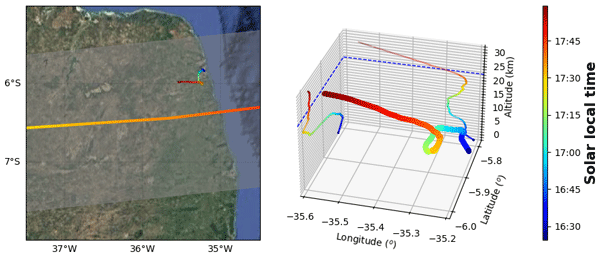
Figure 1 shows the spatial and temporal evolution of the balloon sounding conducted on 14 October 2023 during the annular solar eclipse. The first step to understanding the dynamics involved in these measurements, it was to convert the universal time (UTC) to solar local time (SLT), which depends on the latitude and longitude of the observation points. The same conversion was applied to the temporal evolution of the eclipse path.

Figure 1 The spatial and temporal evolution of the sounding during 14 October 2023 annular solar eclipse is shown above. The left panel displays the coverage of the umbra region, where the color of the central line indicates the corresponding solar local time (SLT), as shown in the color bar. The other colored line, overlaying the Natal region, represents the horizontal path of the balloon, with its color also indicating the solar local time.The right panel illustrate the vertical trajectory of the flight. The dashed blue line marks the exact time and altitude when the elipse passed over the balloon. The map on the left panel was created using Cartopy library (Met Office, 2010–2015).

The SLT is shown in Fig. 1 as the colored lines, one representing the central path of the eclipse and the other showing the trajectory of the balloon over the Natal region. Additionally, the extent of the umbra can be seen as a light gray area in the left panel, where it is clear that the sounding was completely within the eclipse umbra. The right panel shows the vertical evolution of the sounding as a function of latitude and longitude. The dashed blue line indicates the altitude where the eclipse crossed the balloon path.

The balloon was launched at 18:29:44 UTC, and the flight lasted of 5227 s, or ∼ 1.45 h. The eclipse began at 15:03:50 UTC and ended at 20:55:16 UTC. The estimated time for the eclipse umbra to pass over the balloon was 19:50:16 UTC. Notably, the duration of annularity was estimated at 3 min and 36 s. During this interval, the balloon collected about 216 measurements and ascended vertically more than 1.4 km within the shadow of the umbra.

During this flight, it was possible to measure several atmospheric parameters such as pressure, geopotential altitude, temperature, relative humidity, ozone partial pressure, ozone concentration, and wind speed and direction. This experiment was highly unique due to both the eclipse itself, which was annular with an obscuration of around 88.5 % over Natal, and the timing of the flight, which was very close to sunset.

3 Results and discussion

Figure 2 shows vertical temperature profiles for October measured by the balloon flights over Natal (colored lines) and control profiles estimated using the Naval Research Laboratory Mass Spectrometer and Incoherent Scatter model version 2.1 (light gray solid line) and European Centre for Medium-Range Weather Forecasts Reanalysis version 5 (dotted gray line). The average profile for October (dot-dashed olive line) includes all flights during these months from 1999 to 2023 and its standard deviation is represented by the shaded olive area. In addition, the vertical temperature profile obtained on 13 October 2023 (one day before the eclipse) is shown by the dotted blue line while the profile on 14 October 2023 is represented by the solid red line.

Figure 2 Vertical profiles of temperature obtained from stratospheric balloons, the MSIS model and the ERA5 reanalysis. The average profile for all flights conducted during October from 1999 to 2023 is represented by the olive dot-dashed curve, with the shaded olive area showing the standard deviation. The profile collected on 13 October 2023 is represented by the dotted blue line and the profile measured on 14 October 2023 is shown by the solid red line. The dotted gray line show the profile from the ERA5 reanalysis, while the NRLMSISE-00 model is shown by the solid gray line. The inset box in the chart displays the temperature difference between the 14 October 2023 profile and both the MSIS model (dashed gray line) and the climatological October average profile (dashed olive line). The light gray horizontal band with the black dashed line in the center represents the altitude range where the eclipse umbra crossed the path of the balloon. The horizontal cyan areas illustrate regions where statistically significant differences (at a 90 % confidence level) were observed between the profile collected on 14 October 2023 and the climatological mean for October.

In Fig. 2, the horizontal light gray area represents the altitudinal range of the Moon's shadow (umbra), with the dashed black line indicating its center. Figure 2 also includes a small inset box that highlights the altitude range from 14 to 30 km, displaying the differences between the 14 October 2023 profile and both the MSIS and the October average profiles.

The statistical significance of the profile perturbations was calculated using a hypothesis test, assuming that the atmospheric field measurements follow a normal distribution, with the mean and standard deviation calculated from all profiles obtained during the months of October from 1999 to 2023. A 90 % confidence criterion was used to plot the horizontal cyan areas in Fig. 2 and in the subsequent figures presented in this work. As a reference, approximately four balloon launches are conducted per month over Natal, totaling 62 flights, excluding the data from the day of the eclipse.

In the lower troposphere, up to 4–5 km altitude, there are some differences in the profiles when compared to the MSIS control profile. This is probably a response to tropospheric activity, which has strong day-to-day variability. An inversion in the temperature profile is also observed, which is statistically significant compared to the climatological profile. The MSIS model does not predict this inversion, whereas the ERA5 reanalysis profile shows an inversion at the same altitude, but with a smaller amplitude. Between altitudes of 5 and 13 km, the profiles are very close to each other. However, a slight heating on 14 October 2023 was observed compared to the climatological profile.

From 14 km, around the tropopause, pronounced perturbations are visible in both the ERA5 and the observed profiles from 13 and 14 October 2023. Comparing the profile from the day of the eclipse to the others, a distinct cooling in the tropopause was revealed. This cooling reaches about 5 K when compared to the October average profile and more than 4 K relative to the MSIS model. Furthermore, this cooling extended well beyond the standard deviation, making it statistically significant around 18 km altitude. It is worth noting that during this period, the measurements were taken under the influence of the eclipse penumbra, which began over Natal at approximately the time of the balloon launch. Another interesting result was a rise of about 1 km in the tropopause when compared to the climatological data.

Above the tropopause, in the lower stratosphere, variations in the temperature profile measured on 14 October 2023 were observed as compared to the model, reanalysis and climatological profiles. These changes were almost always anti-correlated to the variation observed on the day before the eclipse. Although temperature variations are common at these altitudes, as seen in the individual measured profiles, the oscillation recorded on October 14 stands out because it completely mirrors the patterns of the day before and a significant cooling of ∼ 8 K was observed above 24 km. This cooling is within the altitudinal range statistically significant compared to the overall average. Furthermore, the differences between this specific profile, the October average, and the MSIS models (shown in the small box chart) follow the exact same trend. This strongly indicates that the temperature behavior on 14 October 2023 was unique, directly influenced by the passage of the eclipse.

Changes in Earth's surface temperature are probably among the most studied effects during an eclipse. This is mainly because these measurements are easier collected, either using regular meteorological stations hit by the Moon's shadow or via temporary setups built just for the event. As solar radiation drops, a clear decrease in air temperature is commonly observed (e.g., Founda et al., 2007; Namboodiri et al., 2011).

In contrast, vertical temperature profiles during an eclipse are harder to be investigated because they need a more specific experimental configuration. Nevertheless, some studies have used satellites (e.g., Good, 2016; Paulino et al., 2025; Basha et al., 2025) and vertical soundings (e.g., Harrison et al., 2016; Das et al., 2023; Pasken et al., 2023) to examine how these profiles respond to a local eclipse. In general, researchers have observed cooling and vertical fluctuations in the tropopause, which agrees with our current results. In addition, previous work has also pointed out variations in the tropopause altitude and differences between how land and ocean respond.

Figure 3 is similar to Fig. 2, but displays the atmospheric pressure. The observed profiles are very close to each other and it is difficult to distinguish them in the chart, except for the ERA5 profiles, which were lower than the others, primarily in the upper levels. The small box on the upper left corner emphasizes the region from 9 to 29 km altitude. There it is possible to see that the pressure on 14 October 2023 was slightly lower than the average profile, but higher than the ERA5 data. The difference between the 14 October 2023 profile and the climatological profile decreases with altitude, going from about −0.75 hPa near the tropopause up to the lower stratosphere. This reduction in the pressure is within the confidence level of 99 % based on the climatological records.

Figure 3 Same as Fig. 2, but showing the atmospheric pressure.

Previous observations have reported drops in atmospheric pressure during solar eclipses. For example, Pasken et al. (2023) showed that the pressure reduced slightly during and after the passage of the 21 August 2017 solar eclipse in St. Louis, United States. The temperature gradient produced by the atmospheric cooling can trigger pressure fluctuations with gravity waves as a prominent response (Paulino et al., 2020).

Figure 4 shows the vertical profiles for the Ozone concentration, measured on 13 October 2023 (dotted blue line), 14 October 2023 (solid red line) and the average for October (dot-dashed olive line). The shaded olive area represents the standard deviation of the mean, calculated considering all soundings collected on October from 1999 to 2023. The Ozone concentration below 20 km altitude is very small, less than 1 part per million and the profiles have a lot of oscillation. In this case, two points can be highlighted: (i) a decrease in ozone concentration between approximately 4 and 9 km in altitude and (ii) an increase in ozone concentration between 10 and 14 km in altitude. The observed decrease is almost entirely within the statistically significant region of 90 %, whereas the increase is greater than the average and lies outside the standard deviation region, but has only a few points with 90 % statistical confidence.

Figure 4 Same as Fig. 2, but showing the Ozone concentration. Error bars represent the uncertainties in the ozone concentration discussed in the previous section.

In the stratosphere, it was also observed an increase in ozone concentration above 27.5 km altitude. It reached 1.7 ppm at 29 km, as shown in the zoomed-in box of Fig. 4. This rise in ozone concentration is also statistically significant, since it is within the confidence region of 90 % marked by the cyan area.

Previous studies on total ozone levels during solar eclipses showed an increase of about 4 % in the total ozone column when measured with Dobson spectrophotometers (Fournier d'Albe and Rasool, 1956; Stranz, 1961). Later, Zerefos et al. (2000) found a 30 DU change in ozone concentration caused by diffuse radiation. Mateos et al. (2014) reported a similar trend during the solar eclipse of 3 November 2013 over Spain.

Theoretically, it is expected to see an increase in ozone concentration within the eclipsed column of the atmosphere due to ozone photochemistry. However, a theoretical study revised the enhancement to increase down to 1 % (Hunt, 1965), and more recently, Bernhard et al. (2025) pointed out that the actual change is too small to be measured confidently.

The present observations showed large fluctuations. However, above an altitude of 21 km, just after the passage of the Moon's shadow, the concentration of ozone is practically always higher than it was observed in climatological October over Natal, reaching an increase of a few ppmv in the higher levels. Therefore, these findings match the predictions and represent an interesting result, as the measurements were taken locally and avoid the limitations found in other experiments. This observed increase in ozone concentration of the present work is also supported by previous balloon launches. For instance, a rise of a few ppbv in the troposphere was reported during the 26 December 2019 solar eclipse over Gadanki (Akhil Raj and Ratnam, 2021).

Figure 5 shows the vertical profiles for relative humidity collected during October over Natal. The solid red line represents the measurements on the day of the eclipse. The dotted blue line represents the measurements one day before. The dot-dashed olive line represents the average for October from 1999 to 2023. Again the shaded olive area represents the standard deviation of the mean. Gray dotted line represent the ERA5 reanalysis for the relative humidity on the day of the eclipse. Red error bars represent a rough estimation for the uncertainties for the measurements of relative humidity on 14 October 2023.

Figure 5 Same as Fig. 2, but for relative humidity. The red error bars show an approximate estimation of the uncertainties based on the results of Miloshevich et al. (2009).

The error estimation for relative humidity measurements in SHADOZ launches involves applying empirical correction algorithms to raw radiosonde data to counteract solar radiation dry bias and sensor time-lag under extreme conditions (Miloshevich et al., 2009). Typical residual error is relatively low in the lower troposphere, ranging from ±3 % to ±5 %. However it becomes significant above the tropopause reaching ±10 % to ±20 % due to sensor exposure to temperatures below −40 °C.

Day-to-day variability in the measurements is also very clear for relative humidity. The profile from 14 October 2023 differs significantly from the others, especially above 5 km. From 5 to about 21 km, relative humidity was almost always higher on the day of the eclipse and there were calculated two statistical significant regions, one around 5–7 km and another around 13–14 km.

Above 21 km, which matches the timing of the umbra passing over the balloon, the relative humidity starts to drop, falling below the other measurements. Although the absolute values at these altitudes are very low (less than 1 %) and it was within the standard deviation influence.

Observations in eight Indian cities showed a considerable increase in relative humidity during the 21 June 2020 solar eclipse (Pratap et al., 2021). A similar increase in surface relative humidity was also reported by Tzanis et al. (2008) during the 19 March 2006 solar eclipse in Athens. In contrast, Funari and dos Santos (2018) observed a drop in relative humidity over Brazil during the eclipse of 12 November 1966. More recently, Basha et al. (2025) have also reported an increase in relative humidity over the United States during the 8 April 2024 solar eclipse. In that work, they used data from the COSMIC-2 satellites over both the ocean and land. Their study also revealed fluctuations in the vertical profiles.

During a solar eclipse, the blocking of sunlight is expected to cause an increase in relative humidity, primarily near the surface. This is because evaporation decreases, which subsequently makes the air more humid.

4 Conclusions

During the annular solar eclipse on 14 October 2023, an atmospheric sounding was conducted using a stratospheric balloon over Natal, Brazil. This was a unique experiment due to the geographical region and the nature of the eclipse. The Moon's shadow, creating a “ring of fire”, crossed Natal very close to sunset. The balloon was launched immediately after the penumbra reached the city, collecting atmospheric parameters such as temperature, pressure, relative humidity and ozone concentration for over 1.45 h. The Moon's shadow crossed the balloon at approximately 19:50 UTC when it was at an altitude of about 22.35 km. The eclipse lasted 3 min and 36 s, allowing the instruments to record 216 measurements while the umbra was present. The investigation showed that the atmosphere responds with complex structures and small fluctuations of these atmospheric fields. More specifically, the following was observed:

• Some vertical fluctuations in the temperature profile were observed, with high amplitudes above 14 km. The tropopause experienced a cooling of 4–5 K when compared with the control and average measurements;

• A drop in the pressure of 0.2–0.7 hPa was observed above 12 km altitude, with vertical variations along the altitudes;

• The ozone concentration presented many vertical oscillations, and an increase above 20 km reaching 1.7 ppm was observed;

• Between 5 and 18 km of altitude, the relative humidity increased compared to the control profiles.

All the experimental results are in agreement with previous observations and are consistent with the expected effects of the solar eclipse on the atmosphere. This supports the interpretation about the importance of the annular solar eclipse as a transient event affecting the local structure and dynamics of the atmosphere.