High-latitude MSTIDs over the EISCAT-3D site: solar activity and seasonal dependency

This work involves an investigation of high-latitude medium scale traveling ionospheric disturbances (MSTIDs) over the newly established EISCAT-3D radar site. We have used the ground backscatter data from an HF radar located at Hankasalmi, Finland (∼62.3° N, ∼26.61° E geographic coordinates), which is a part of the SuperDARN (Super Dual Auroral Radar Network). Data from solar maximum (2001 & 2014) and minimum (1996 & 2009) years from solar cycles 23 and 24 have been used to investigate the characteristics, seasonal variation, and possible generating sources of high-latitude daytime MSTIDs. Irrespective of the seasons and solar activity conditions, a dominant fraction of MSTIDs propagates equatorward with velocity in the range of 50–150 m s⁻¹ and period in the range of 30–60 min. Their occurrence shows seasonal and solar activity dependency. They normally occur during winter and equinoctial months. During solar maximum conditions, the occurrence is comparatively higher (∼72 %) than during solar minimum years (below 50 %). Furthermore, the MSTIDs' occurrence shows a dependence on IMF B_z, being generally higher during intervals of prolonged northward or southward IMF B_z, and lower during small or fluctuating IMF B_z conditions. Our results indicate that MSTIDs occurrence shows seasonal variation as well as dependence on the solar forcing. Therefore, this statistical study will help in providing comprehensive insight about the MSTIDs which will be effective in scheduling future experimental runs of EISCAT-3D to explore their 3-dimensional structures.

1 Introduction

Traveling ionospheric disturbances (TIDs) are propagating electron density perturbations in the ionosphere. They pose a persistent challenge due to their ability to severely affect radio propagation, often leading to disruption of radio-communications, increased convergence time of the precise point positioning of Global Navigation Satellite Systems (GNSS), and distortion of radio signals from astronomical sources (Boyde et al., 2025; Carter et al., 2023; Maletckii and Astafyeva, 2024). They are believed to be the manifestation of atmospheric gravity waves (Hines, 1960; Hocke and Schlegel, 1996; Hunsucker, 1982). Based on their scale sizes, TIDs are categorized as large, medium, and small scale (Hunsucker, 1982). Large scale TIDs (LSTIDs) having wavelengths of more than 1000 km, propagate towards the equator with a velocity in the range of 400–1000 m s⁻¹, have a period of more than 1 h and are mostly generated by geomagnetic activity in the auroral region (Ding et al., 2008; Tsugawa et al., 2004). Small scale TIDs (SSTIDs) have wavelengths less than 100 km and are usually generated by lower atmospheric gravity waves (Boyde et al., 2022). Medium scale TIDs (MSTIDs) normally propagate equatorward with a velocity of a few hundred m s⁻¹, a period in the range of 30–60 min, and wavelength of a few hundred km (Grocott et al., 2013; Hocke and Schlegel, 1996; Huang et al., 2016; Ishida et al., 2008; Rathi et al., 2025; Shiokawa et al., 2003) and are believed to be generated by various sources (e.g., external solar forcing, internal atmospheric forcing, and natural hazards).

MSTIDs have been observed and reported over both mid and high-latitude regions (Grocott et al., 2013; Huang et al., 2016; Ishida et al., 2008; Shiokawa et al., 2003). Mid-latitude MSTIDs have been investigated extensively, and observations indicate that they generally occur during geomagnetic quiet time (Ding et al., 2011; Huang et al., 2016), whereas MSTIDs over high latitudes occur during both geomagnetic quiet and active times. They are believed to be generated by multiple sources such as Joule heating by geomagnetic storms and substorms, gravity waves generated by tropospheric convection, and the solar terminator (Grocott et al., 2013; Ishida et al., 2008; Prikryl et al., 2022, 2025). There are studies which explored high-latitude MSTIDs utilizing datasets from various ground and satellite-based instruments over both hemispheres (Frissell et al., 2016; Grocott et al., 2013; Ishida et al., 2008; Negale et al., 2018; Ogawa et al., 1987; Prikryl et al., 2022, 2025; Shiokawa et al., 2013; Vlasov et al., 2011; Xiong et al., 2025). These studies reported MSTIDs that normally propagate towards the equator and whose occurrence shows seasonal variation. However, a lack of agreement exists in the observed seasonal dependence; with peak occurrence in both summer (Vlasov et al., 2011) and winter (Moges et al., 2024b; Negale et al., 2018; Ogawa et al., 1987) months. In addition, there are two schools of thought on their generation with respect to geomagnetic activity. There are studies which reported high-latitude MSTIDs during geomagnetic quiet and/or moderately disturbed times and suggested that the occurrence of these MSTIDs did not increase with increasing geomagnetic activity (Frissell et al., 2016; Ishida et al., 2008; Ogawa et al., 1987). On the other hand, Prikryl et al. (2022, 2025) reported that MSTIDs over high-latitudes can also be generated by atmospheric gravity waves induced through Joule heating by external solar forcing (geomagnetic storms and/or substorms). More recently, Xiong et al. (2025) reported that high-latitude daytime MSTIDs can also be observed during prolonged northward IMF B_z conditions and explored the possible role of intermittent lobe reconnection behind their generation. It is thus very apparent that a wide variety of generation or seeding mechanisms are associated with high-latitude MSTIDs. However, there is still much uncertainty surrounding their seasonal variation and the conditions that make a particular mechanism dominant.

This study aims to explore the seasonal variation and generating sources of the high-latitude MSTIDs using ground backscatter data of the Hankasalmi radar. The rationale behind selecting the Hankasalmi radar is the geographic location and the operational range that coincides partially with the newly established EISCAT-3D radar. EISCAT-3D is the most advanced high power three-dimensional imaging radar for atmospheric, ionospheric, and near-Earth space investigations. Since it requires high power and high cost for experimental runs, a prior understanding of ionospheric irregularities (e.g., their characteristics, occurrence patterns with respect to season and external solar forcing) is required before its operational phase. In order to deepen our understanding, we have investigated daytime MSTIDs during solar maximum (2001 & 2009) and minimum years (1996 & 2009) from solar cycles 23–24 over this region and have used different approaches to characterize the observed MSTIDs while also investigating the role of external solar forcing behind their occurrence.

2 Instruments, Data, and Analyses Methods

In the present study, we have used the data from an HF radar located at Hankasalmi, Finland (∼62.3° N, ∼26.61° E geographic coordinates). The Hankasalmi radar (hereafter HAN) is a part of the SuperDARN (Super Dual Auroral Radar Network), an international array of coherent radars in the Northern and Southern Hemispheres (Greenwald et al., 1995; Chisham et al., 2007). In the normal mode of operation, the HAN radar uses 16 beams for scanning with azimuthal separation of 3.24°, where each beam typically consists of 75 range gates of size 45 km, with the first range gate sampling at 180 km from the radar location (for a full field of view thus spanning ∼3500 km). Each beam typically has a dwell time of ∼3 s and thus the radar completes a full 16 beam scan in ∼1 min (in the initial phase of operation the radar had dwell time of ∼7 s with a full scan in ∼2 min).

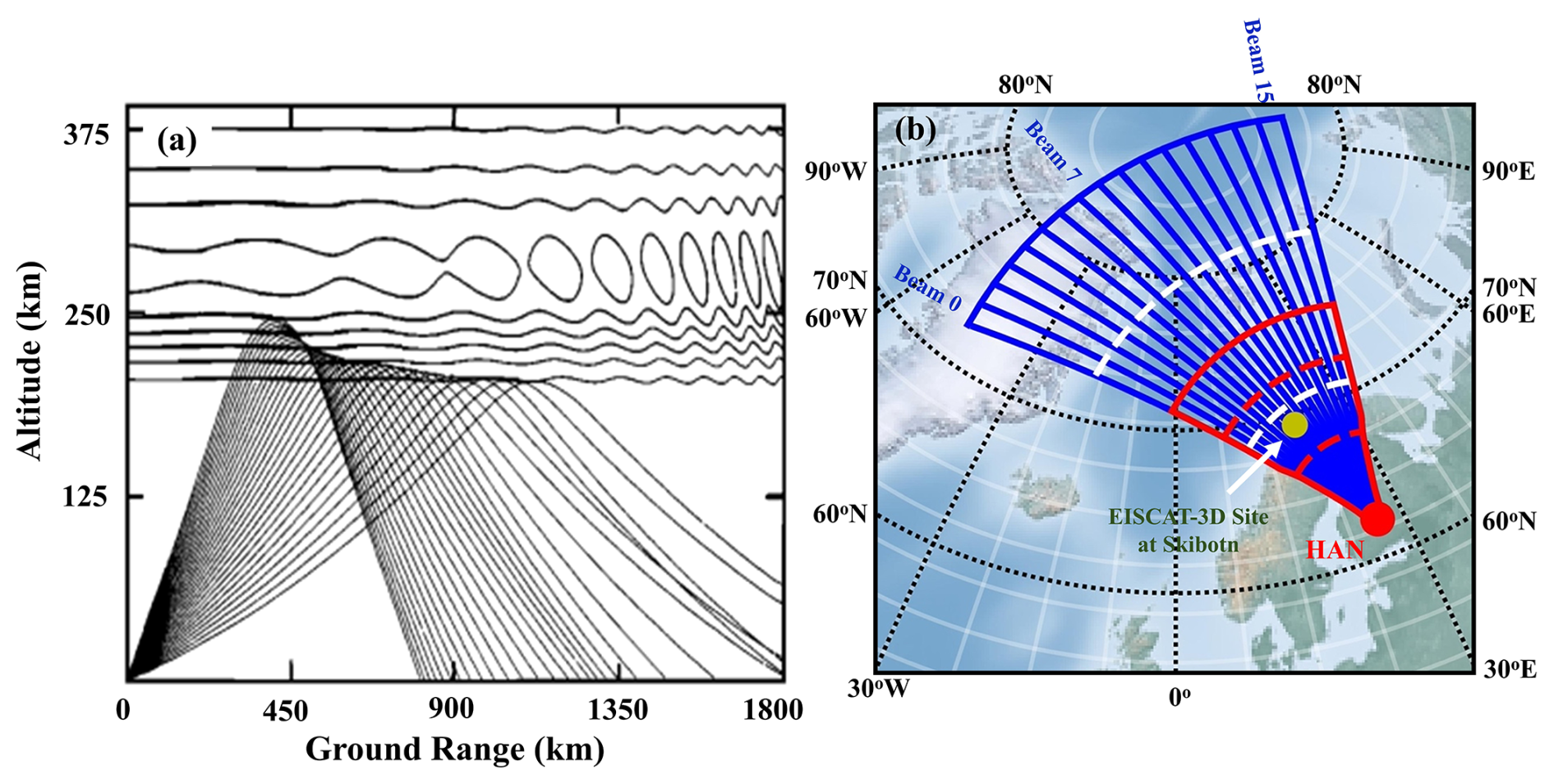
Figure 1 (a) Model ray paths of HF propagation through a TID modulated ionosphere (adapted from Samson et al., 1990). (b) Field of view (FOV) of HAN radar in GBS ranges (blue FAN plot) and ionospheric mapped ranges (red FAN plot). The red and yellow dots show the locations of the HAN radar and EISCAT-3D at Skibotn, respectively. HAN radar range gates 20 and 45 (bounding the area under study) are indicated by the white dashed (GBS ranges) and red dashed (mapped ranges) curves.

A SuperDARN radar works on the principle of coherent scattering and receives backscatter signals from the ionosphere as well as from the ground. Such radars receive ionospheric backscatter if the transmitted signal intersects with the ionospheric target orthogonally to the magnetic field (achieved through ionospheric refraction of the signal). Further refraction of the signals directs the transmitted signals to the ground, from which they can propagate back to the radar. This is known as ground backscatter (GBS). Modulations/fluctuations in ionospheric plasma density caused by MSTIDs affect the GBS by focussing/defocussing of the signals (Grocott et al., 2013; Samson et al., 1989, 1990) as shown in Fig. 1a. It is apparent from the figure that the location of the TID signature in GBS will be displaced from its actual location at the ionospheric height. Therefore, we have mapped the GBS to the ionosphere using the standard geolocation functions in the pyDARN python library (SuperDARN Data Visualization Working Group, 2025) to estimate the location of the observed MSTIDs. The field of view (FOV) of the HAN radar in GBS ranges is represented by the blue FAN plot whereas the red FAN plot represents the mapped ionospheric ranges in Fig. 1b. The location of the HAN radar and EISCAT-3D at Skibotn, Norway are represented by the red and yellow dots, respectively. EISCAT-3D is located close to beam 7 (the nearly northward pointing beam) of the HAN radar. Therefore, in this study we have used data from beam 7 (as the central beam) in our analysis. We also restrict the analysis to radar range gates 20–45, which is the region where the maximum amount of radar ground backscatter was observed. This region is confined between the white dashed curves (in GBS ranges) and red dashed curves (in mapped ranges) in Fig. 1b.

MSTIDs observed between 60 and 90° latitude are categorized as high-latitude MSTIDs. As the HAN radar probes the same ionospheric region (as shown by its FOV in Fig. 1b), the main objective of this study is to investigate the propagation characteristics and occurrence of high-latitude MSTIDs during different solar activity conditions. We have therefore used HAN GBS data for solar minimum (1996 & 2009) and maximum (2001 & 2014) years from solar cycles 23 and 24. To determine the propagation characteristics, viz. velocity, period, and direction of propagation [azimuth angle (clockwise from geographic north)] of the observed MSTIDs in the GBS, the multichannel maximum entropy method (MULMEM) has been used (Grocott et al., 2013; Ishida et al., 2008; Shibata, 1987; Strand, 1977; Ulrych and Bishop, 1975). This method uses cross-spectral analysis to determine the parameters of MSTIDs from the GBS time series. We note that GBS depends on the ionospheric plasma density which reduces significantly during nighttime (Milan et al., 1997), therefore, the present study focusses on daytime MSTIDs observed in the GBS.

MSTIDs have periods of ∼30–60 min, therefore, we have performed the MULMEM analysis on a window of 160 min, such that it covers at least 2–3 wave periods. The analysis is then performed across an 8 h time series with the window shifted in 1 min increments. Each overlapping window segment produces a set of propagation parameters/characteristics [period, velocity and azimuth (clockwise from geographic north)] that is attributed to the centre time of the window, therefore with each slide of this window we build up a time-series of parameters. The MULMEM algorithm uses three time series from three radar cells (combination of beams and range gates) to determine these propagation characteristics of the observed MSTIDs. The location of EISCAT-3D at Skibotn lies within the beam 7 of HAN radar, therefore, in the present study we considered beam set (5, 7, 9). The range gates are chosen based on the region of higher GBS occurrence and it is seen that, during daytime, consistently higher GBS was observed between range gates 20 and 45. Therefore, our chosen combinations of the beam-range sets (cells) are [(5, r); (7, r+4); (9, r)], where r (range gates) varies from 20 to 45. To detect the existence of MSTIDs, the MULMEM method first checks whether the GBS time series data is continuous or not. A time series comprising non-continuous data is considered unfit to be processed further. After the initial check, the time series of period values is calculated using cross-spectral analysis and is followed by calculating the concordance rate, where the number of determined period values is divided by total data points in the time series of period. When the concordance rate is greater than 10 % (to remove the cases with very few MSTID detections), the algorithm proceeds with the presence/existence of a TID. Once the presence of a TID in the time series is confirmed, the algorithm determines the propagation parameters/characteristics. Using cross spectral analysis, it determines the dominant period within the time window (160 min). In selecting the dominant period for each time window, it checks and only considers if the dominant period across all the three time windows is within ±5 min. Then it evaluates the velocity and azimuth after estimating the separation and time delay between the cells. The window is then shifted and the cross-spectral analysis repeated. Ultimately, a set of three time-series of parameters is produced for each three-cell set, from which a mean time-series of parameters is derived for each cell set. To estimate the uncertainty of the parameters we have determined their standard deviation across the three time series for every MSTID event. The maximum uncertainty across the considered four years in period, velocity, and azimuth is observed to be 12 %, 9.5 %, and 9.8 % of the respective average values. We further considered if the presence of a MSTID is detected in multiple three-cell sets. In those cases, we again checked the standard deviation of the parameters across all the cell sets at each time. For such cases where parameters show similar values (with standard deviation <20 %) for different cell sets, we consider those as single MSTID events. Figure 2a shows an example (on 27 January 2014) of such cases where parameters are nearly the same in different cell sets and count as a single MSTID event.

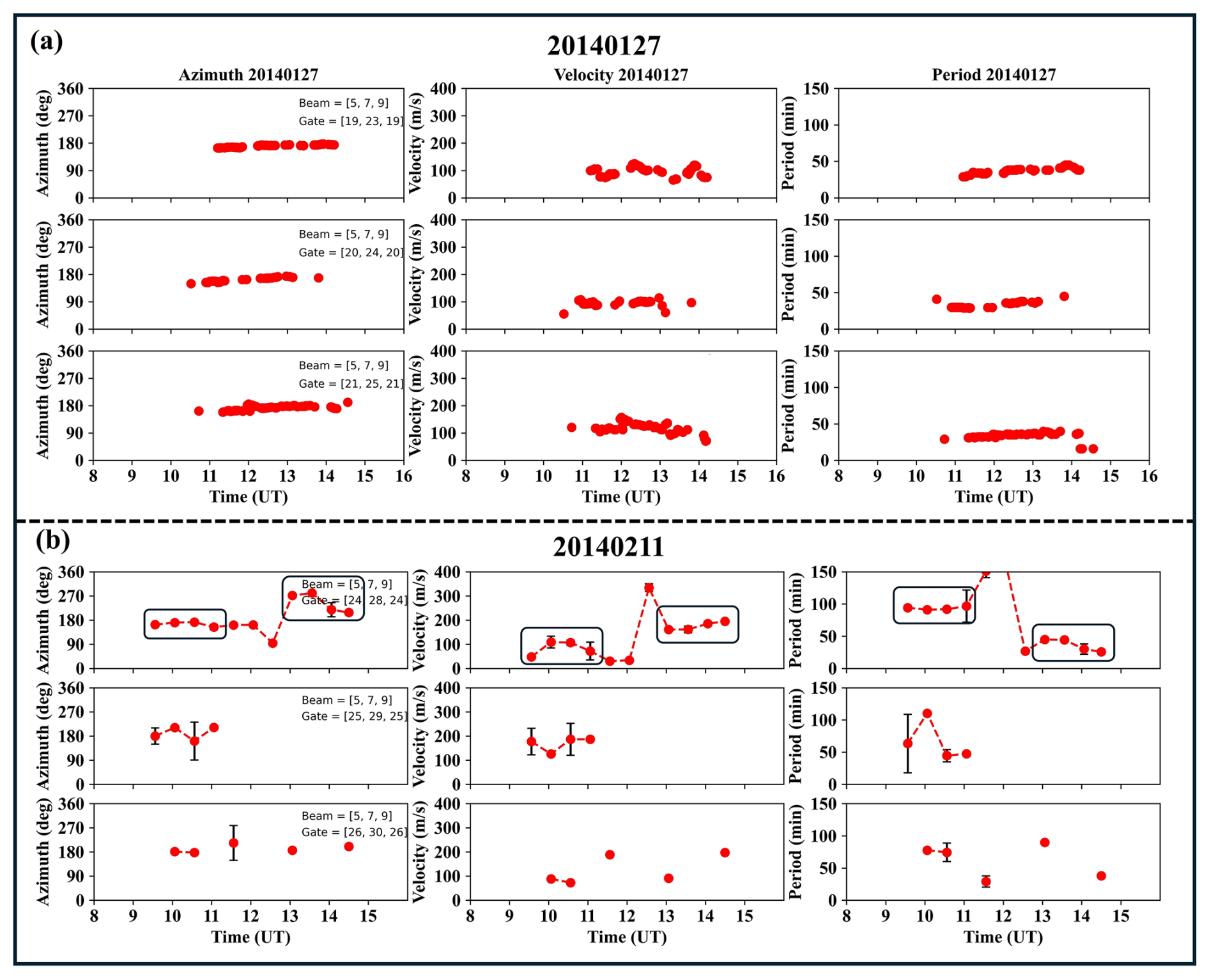
Figure 2 Parameters (azimuth, velocity, and period) determined using MULMEM for the MSTIDs observed on two different days; (a) on 27 January 2014 and (b) on 11 February 2014. The black rectangles in subfigure (b) represents the parameters of two different MSTIDs observed on the same day.

A separate half an hour non-overlapping window is considered to check temporal variations in the parameters by assessing the mean and standard deviation of each window. Figure 2b is representative of this analysis, where average parameters for every half an hour window and their standard deviation (shown by error bars) are plotted for different cell sets. For the first cell set (first row of Fig. 2b), two different values of the parameters are observed (marked with black rectangles) for different time ranges. In such scenarios, where parameters show two different values (azimuth difference ≥90°; velocity & period difference ≥ double) either with time and/or different cell sets, we count them as two different MSTIDs. Also, we checked the standard deviation of each half an hour window and made sure it is less than 20 % of the average value for each parameter. The number of such cases are few and in most of those cases MSTIDs are observed at different times. The cases where the parameters show high temporal variations/fluctuations (Azimuth ≥45°; Velocity ≥50 m s⁻¹; Period ≥15 min) with larger standard deviations ($\ge \pm \mathrm{20}$ % of the values) and/or scattered values with time (as shown in second and third row of Fig. 2b) are not considered/counted.

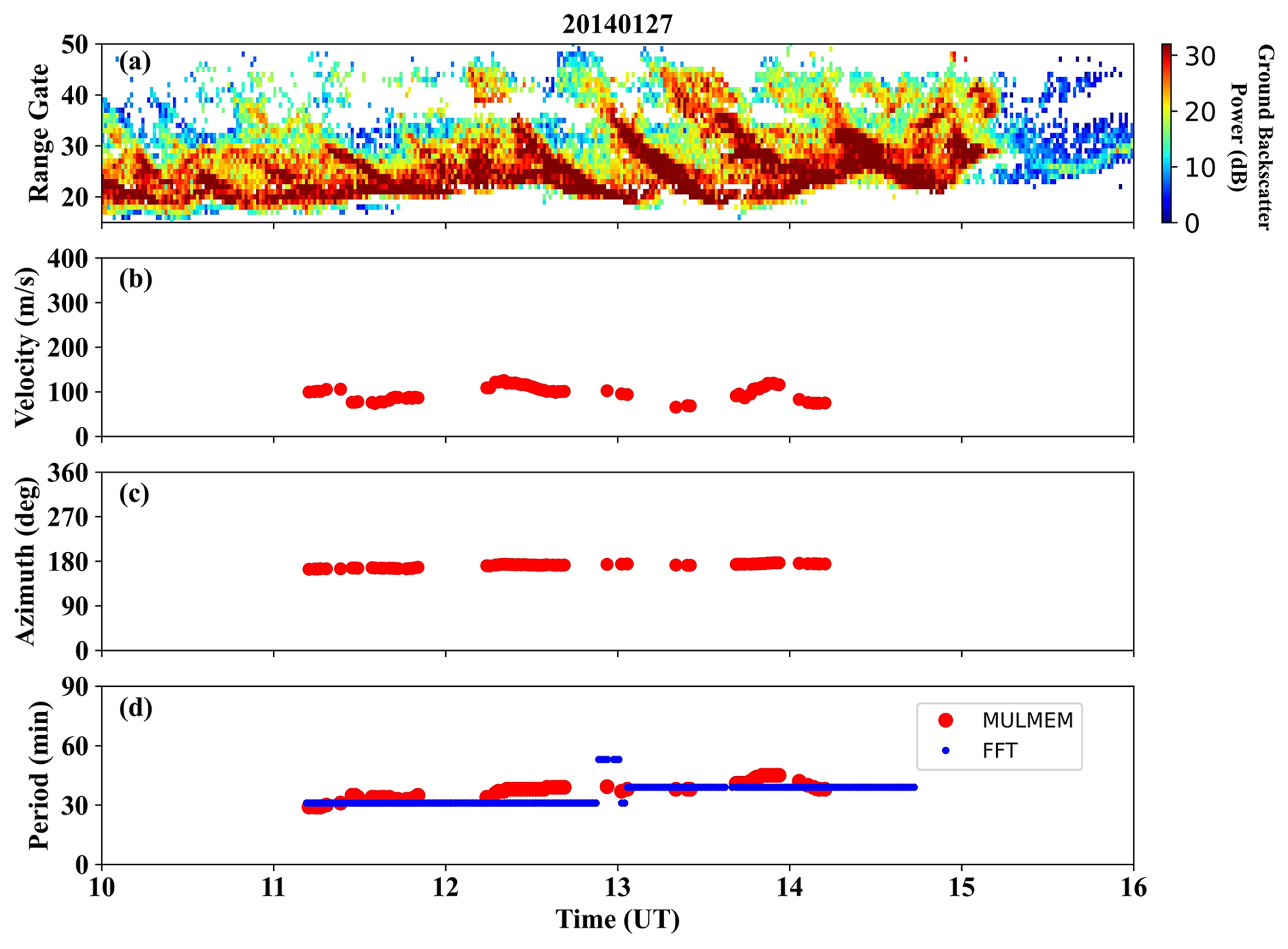
Figure 3 (a) An example showing MSTID in RT plot, (b–c) velocity and azimuth angle (clockwise from geographic north) determined using MULMEM, (d) comparison of period determined using MULMEM (red curve) and FFT (blue curve).

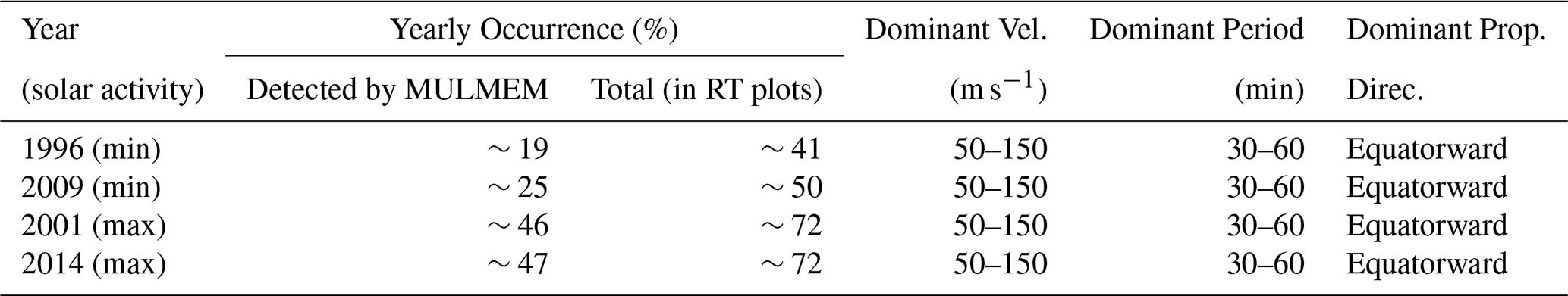
MSTIDs cause focussing/defocussing of SuperDARN GBS, therefore they appear as bands of high GBS. To confirm the presence of MSTIDs and their propagation, we have also checked the Range Time (RT) (e.g. Fig. 3a) and FAN (which shows spatial coverage of GBS power across the radar's FOV, see Fig. S1 in the Supplement) plots for each case. In the present study we have visually inspected the RT plots for MSTID signatures and compared them with the results obtained from MULMEM. As mentioned above, due to the detection approach of MULMEM there are instances where the method failed to identify MSTIDs when cross checked with the RT plots (Table 1). We presume this is due to the requirement for a clear signal to be present in the 3 radar cells. In many of these cases, a signal was present in at least one cell, enabling a Fast Fourier Transform (FFT) analysis to determine a dominant period. For all the MSTID events observed in the RT plots we therefore also performed an FFT analysis to determine their period (using the same window size from the time series of beam 7) by selecting time series between the range gates 20 and 45 (as selected for MULMEM). Figure 3 shows an example MSTID (Fig. 3a), and its parameters obtained from MULMEM (red curves in Fig. 3b–d: velocity, azimuth angle, & period) & FFT (blue curve in Fig. 3d: period). We have also provided a comparison of the MSTIDs detected using the MULMEM analysis, and the total number of MSTIDs observed in the RT plots for each year (see Table 1).

Table 1 Showing the year wise MSTIDs' percentage occurrence (detected by MULMEM and total observed in the RT plots) and their dominant characteristics (velocity, period, & azimuth).

3 Results

This section presents a statistical overview of the high-latitude daytime MSTIDs observed during different solar activity conditions. As described in the previous section, we have applied different methods to detect and determine their characteristics. A detailed description about their occurrence and characteristics is given below.

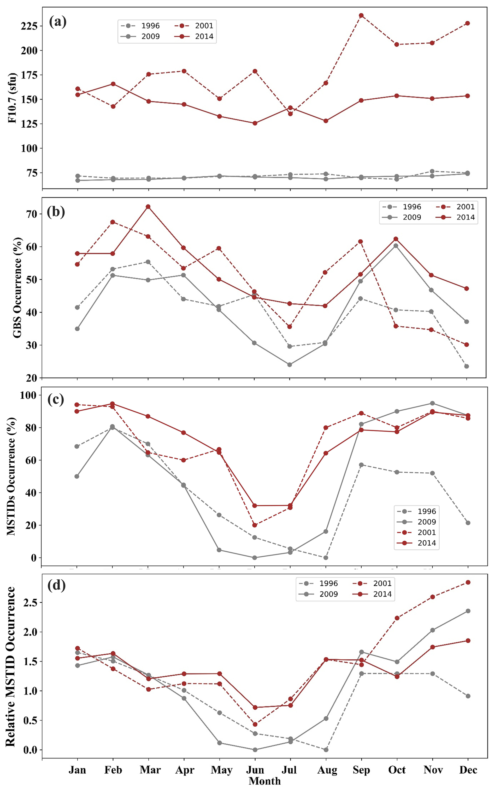
Figure 4 (a) Monthly average F10.7 index, (b) monthly % occurrence of ground backscatter, (c) monthly % occurrence of the MSTIDs, and (d) relative occurrence of MSTIDs with respect to GBS occurrence during solar minimum and maximum years of solar cycle 23 and 24.

3.1 Seasonal and solar activity dependence of MSTIDs' occurrence

As observed and reported earlier, SuperDARN GBS depends on a number of factors including the refraction and absorption of the transmitted signal, the occurrence of plasma structures, and the ionospheric density. In general, the higher the ionospheric density the greater will be the level (signal to noise ratio) of GBS (Milan et al., 1997). In the present study, due to higher ionospheric density in the daytime and thus higher GBS, we have considered the daytime observations from the HAN radar during the selected four years. As daytime extends for different time lengths depending upon seasons, therefore, we have considered a fixed time window between 09:00 and 17:00 LT (close to the beam 7 observation region) across all seasons. Figure 4 shows the variation of monthly average F10.7 index, percentage occurrence of GBS, and MSTIDs percentage and relative occurrence. In each subfigure, the maroon and grey curves show the variation during solar maximum (dashed for 2001 & solid for 2014) and minimum (dashed for 1996 & solid for 2009) years, respectively. Figure 4a shows the monthly variation of F10.7 index, which was comparatively higher during solar maximum years (2001 & 2014) than during minimum years (1996 & 2009). Figure 4b shows the variation of the monthly percentage occurrence of daytime GBS of beam 7. The GBS monthly percentage occurrence was determined by dividing the number of bins (time and range gate bin) where GBS was present (GBS power >0) by the total number of bins for time range 08:00–16::00 UT and range gate 20–45 for each day (when the radar was operating in its normal mode) of the respective month. It is to be noted that, irrespective of the solar activity conditions, GBS occurrence across all the years shows a seasonal variation. GBS occurrence is comparatively higher in the winter and equinoctial months, but it reduces significantly in the summer. In addition to the seasonal variation, GBS occurrence shows a solar activity dependence. It is higher during the solar maximum years (maroon curves) than during the minimum years (grey curves). Figure 4c shows the monthly percentage occurrence of MSTIDs, calculated as the total number of days with MSTIDs activity observed in GBS for each month with respect to the total number of days the HAN radar was operational (in normal mode) for that particular month. The occurrence of MSTIDs shows a similar pattern to the GBS occurrence, with a significantly higher occurrence during solar maximum years, and during winter and equinoctial months, compared to solar minimum years and summer months. It can also be seen from Table 1 that the occurrence of MSTIDs is more than 70 % during solar maximum years (2001 & 2014), whereas it reduces below 50 % during the solar minimum years (1996 & 2009). Figure 4b and c show that both GBS and MSTIDs occurrence exhibits seasonal variation. Therefore, there is a chance that the MSTID seasonal variation might have been influenced by the GBS seasonal variation. We have thus determined the relative occurrence (see Fig. 4d) of the MSTIDs with respect to GBS occurrence, which was determined by dividing the MSTIDs percentage occurrence for each month with the percentage occurrence of GBS for the respective month. It is interesting to note that, similar to the GBS and MSTID occurrence, MSTIDs relative occurrence also shows a seasonal variation.

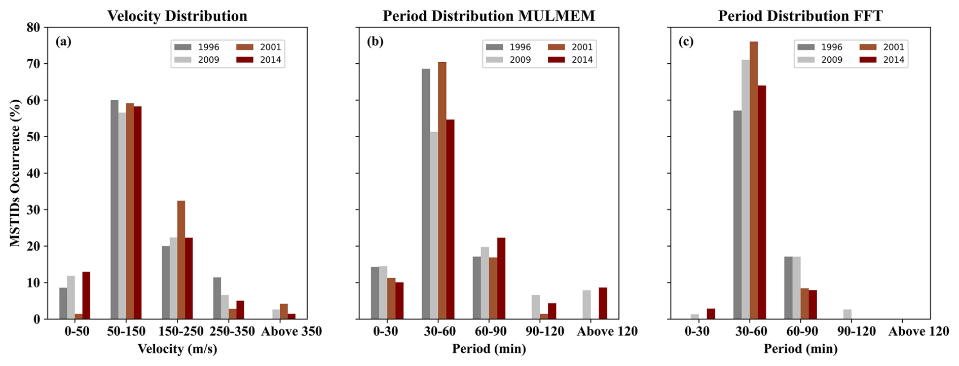
Figure 5 Velocity and period distribution of the MSTIDs observed during the four years of the two solar cycles.

3.2 Characteristics of MSTIDs

Figure 5 presents bar plots of the velocity and period distribution of the observed MSTIDs from the MULMEM and FFT analyses described above. The bar plots in brown & maroon show the MSTIDs' percentage occurrence (obtained by dividing the number of MSTIDs in each group of velocity/period to the total number of MSTIDs observed in the respective year) during solar maximum years (2001 & 2014), whereas dark & light grey bars show MSTIDs during solar minimum years (1996 & 2009). Figure 5a shows the velocity distribution obtained using the MULMEM method, which is distributed in 5 velocity groups (0–50, 50–150, 150–250, 250–350, & above 350; in m s⁻¹). It can be inferred from the velocity distribution that irrespective of the solar activity conditions (across 4 years), ∼60 % of the MSTIDs propagates in the velocity range 50–150 m s⁻¹. The second dominant fraction (more than 20 %) of MSTIDs propagates with velocity in the range of 150–250 m s⁻¹. Figure 5b–c show the period distribution determined using both MULMEM and FFT methods. This shows that irrespective of the methods and solar activity conditions, most of the MSTIDs have a period in the range of 30–60 min, whereas the second dominant fraction has a period in the range of 60–90 min.

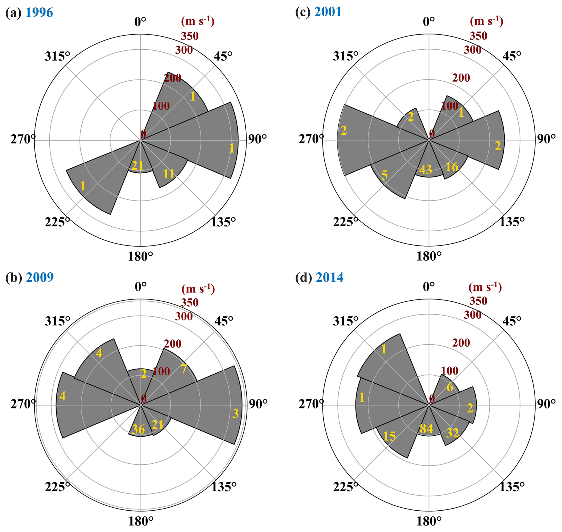
Figure 6 Distribution of the azimuth angle of MSTIDs, number of MSTIDs in each azimuth range (yellow values), and their average velocity (radial axis, labelled with red values).

Figure 6 shows the distribution of the azimuth angle of the observed MSTIDs. The azimuth is distributed in 8 groups with each group covering an angle range of 45° (centred at 45, 90, 135, 180, 225, 270, 315, & 360°). Each circle in the plots represents the magnitude of the velocity in an increasing order from the centre (each circle marked with the magnitude of the velocity in red font with 0 m s⁻¹ at the centre). The grey shaded areas represent the different azimuth ranges, and their extension represents the average velocity of the MSTIDs traveling in those directions. The numbers of MSTIDs traveling in each azimuth range are marked by the yellow font on each shaded area. We can infer that, regardless of the solar activity conditions, a dominant fraction of the observed MSTIDs propagates equatorward (southward) with a second dominant fraction propagating southeastward. There is a very small number of MSTIDs traveling towards north, east, and west. It is also interesting to note that the MSTIDs propagating meridionally (equatorward and/or poleward) has lower velocity compared to those propagating zonally (eastward and/or westward). However, there is a distinct imbalance in the number of zonally and meridionally propagating MSTIDs, therefore, comparison may provide biased results. We have thus performed the significance test (Fisher Exact test) for the obtained results. Fisher Exact test is a statistical procedure to determine the probabilities (p value) of categorial variables (Fisher, 1935), which works with the initial consideration that categories are independent. In the present study, we have used this test between two categories (meridionally and zonally propagating MSTIDs) and we found that differing velocities of zonally and meridionally propagating MSTIDs is significant (p value <0.0001). Table 1 also shows the dominant parameters (velocity range, period range, and azimuth angle) of the MSTIDs during all the four years. In addition, we have also assessed the characteristics with respect to seasons, however, we did not find any significant dependency on seasons observed in their occurrence (figure not provided).

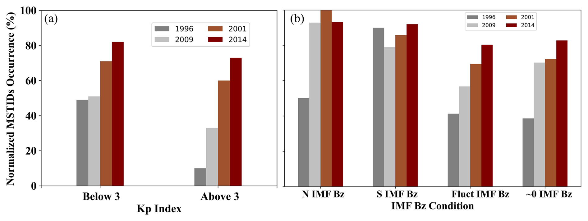
Figure 7 (a) Shows the distribution of the MSTIDs normalized with respect to Kp index. (b) Shows the distribution of the MSTIDs normalized with respect to different IMF B_z conditions.

3.3 Solar wind driver and geomagnetic activity dependence of MSTIDs

We have further investigated the MSTID occurrence with respect to different Kp index levels and IMF B_z conditions, shown in Fig. 7. We grouped the MSTIDs with respect to Kp; with Kp ≥3 (geomagnetically active times) and Kp <3 (geomagnetically quiet times). Their normalized percentage occurrence (obtained by dividing the number of MSTIDs in each Kp group to the total number of days within the respective group) is presented in Fig. 7a. In both the categories, the occurrence of the MSTIDs is comparatively high during solar maximum years, consistent with their occurrence having a direct dependency on solar activity. In order to check the variability of MSTID occurrence with respect to IMF B_z conditions, we segregated and normalized the MSTIDs into four groups designated as close to zero, prolonged northward, prolonged southward, and fluctuating IMF B_z. The segregation is done based on its behaviour in the considered time window of 08:00–16:00 UT with the following criteria: If the temporal average and standard deviation (std) of IMF B_z is within ±1.5 nT, it is considered as “close to zero”. For “prolonged northward”, if the temporal average is greater than 1.5 nT with 80 % of the IMF B_z values lying northward (>1.5 nT) and remaining northward for at least 2 h or more. For “prolonged southward”, if the temporal average is less than −1.5 nT with 80 % of the IMF B_z values lying southward ($<-\mathrm{1.5}$ nT) and remaining southward for at least 2 h or more. For “fluctuating IMF”, the temporal average and std of IMF B_z is within ±2 nT and more than ±1.5 nT respectively with IMF B_z continuously fluctuating between north and south. The normalization is done by dividing the number of MSTIDs in a particular IMF B_z category to the total number of days within the respective category for each year. Figure 7b shows the distribution of the normalized MSTID occurrence (%) with respect to each category. It is evident that irrespective of the categories of IMF B_z, MSTID occurrence is higher during solar maximum than during minimum years (Fig. 7b and Table 2). It is interesting to note that MSTID occurrence is comparatively high during prolonged northward and southward IMF B_z conditions (excepting the 1996 minimum). During solar maximum years intervals of steady B_z conditions has more than 80 % MSTID occurrence (100 % during the 2001 maximum). Fisher exact significance test (applied on the number of MSTIDs under maximum and minimum year categories) also confirms the results are significant with p value less than 0.05. Small B_z or fluctuating B_z conditions tended to yield relatively few MSTIDs.

Table 2 MSTIDs' normalized percentage occurrence with respect to Kp index and IMF B_z.

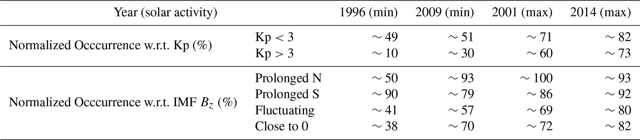
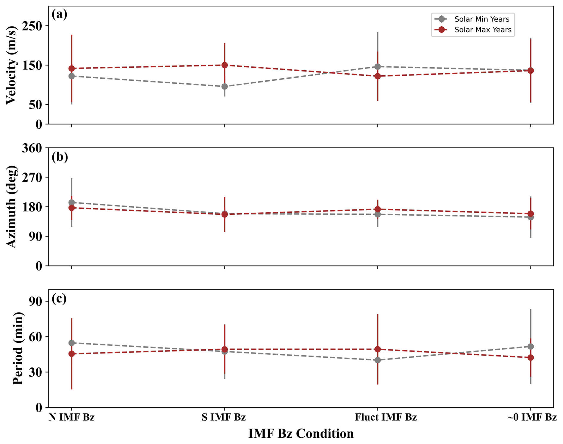
Figure 8 Shows the variability of the MSTIDs' average parameters during solar maximum (maroon curves) and minimum (grey curves) years under different IMF B_z conditions.

We have further checked the variability of the MSTIDs' parameters with respect to different Kp index and IMF B_z conditions. The parameters do not show any variability with different Kp index conditions (figure not provided). Figure 8 shows the MSTIDs' average parameters (velocity, azimuth angle, and period) for different IMF B_z conditions during solar maximum (maroon curve) and minimum (grey curve) years. The parameters do not show significant variability with respect to solar activity and IMF B_z conditions. There is a relatively high velocity under steady IMF B_z (Northward and Southward) conditions during solar maximum years (Fig. 8a). It is also noted that average values of the parameters in each IMF B_z category of solar max years are within 1σ values (shown by error bars) of the solar min years and vice-versa and in the dominant parameter ranges as shown in Figs. 5 and 6 and Table 1.

4 Discussion

In the previous section, we have described the characteristics and occurrence of high-latitude MSTIDs observed over the EISCAT 3D site location and how they vary with different levels of solar activity and with season. We can infer that most of the MSTIDs propagates equatorward (southward) with dominant velocity in the range of 50–150 m s⁻¹ and period in the range of 30–60 min. Their occurrence shows seasonal variation; they normally occur during winter and equinoctial months. We have also observed that with increasing solar activity the MSTID occurrence increases (Fig. 4 and Table 1). In this section we discuss the role of solar forcing in the generation of MSTIDs. In addition, we also compare the results obtained by the MULMEM and FFT method.

4.1 Drivers behind the generation of high-latitude MSTIDs

Daytime high-latitude MSTIDs are analysed to examine their occurrence and possible generating sources. While previous works have reported their seasonal variations and proposed several generation mechanisms (such as geomagnetic forcing and atmospheric gravity waves), the dominant source remains uncertain. We investigated their occurrence with respect to different seasons and solar activity conditions. Our observations show a clear seasonal variation (Fig. 4), with occurrence highest during winter and equinoctial months and lower during summer. This pattern agrees with earlier reports of winter maxima at high latitudes (Moges et al., 2024b; Negale et al., 2018; Ogawa et al., 1987) and contrasts with summer peaks found in other studies (e.g. Vlasov et al., 2011). These studies investigated MSTIDs occurrence utilizing datasets from different instruments such as ionosonde, incoherent scatter radars, NNSS (Navy Navigation Satellite System) satellites, etc. The similarity between the present seasonal pattern and that of atmospheric gravity wave activity in the Arctic (Hei et al., 2008; Hoffmann et al., 2013; Yoshiki and Sato, 2000) suggests that gravity waves propagating upward from the lower atmosphere may contribute to MSTIDs generation. However, the transmission of such waves is influenced by stratospheric and mesospheric filtering (Boyde et al., 2025) and possible dissipation at critical levels (Fritts and Vadas, 2008; Vadas, 2007). Confirmation of their role will require dedicated ray-tracing studies to identify specific sources and propagation paths.

In addition to the seasonal variation, MSTIDs occurrence also varies with solar activity (Fig. 4c, Table 1), increasing from below 50 % during solar minima to more than 70 % during solar maxima. This behaviour broadly reflects the enhanced geomagnetic activity associated with higher solar flux. Previous studies have disagreed on the extent of geomagnetic control – some linking MSTIDs to Joule heating from storms and substorms (Prikryl et al., 2022, 2025), others noting frequent events during geomagnetically quiet times (Frissell et al., 2016; Ishida et al., 2008). Recently, Moges et al. (2024a) investigated MSTIDs amplitude-solar activity dependence and suggested that over high-latitudes the dependency is quite complex involving multiple mechanisms together. Our results show that the occurrence of high-latitude MSTIDs increases with increasing solar activity. We have further investigated their occurrence with respect to different Kp index levels (Fig. 7a). However, there is a modest increase in their occurrence during geomagnetic quiet times (Kp <3), even during solar maximum year, suggesting that Kp alone is not a good indicator of MSTIDs occurrence. This implies that there are other factors/sources that might be responsible for their generation.

Recently, Xiong et al. (2025) reported an interesting case of daytime high-latitude MSTIDs during a geomagnetic quiet period of prolonged northward IMF B_z suggesting that Joule heating due to intermittent lobe reconnection can also be a possible factor for their generation. To explore the influence of IMF orientation, we have examined the role of different IMF B_z conditions (prolonged northward, southward, fluctuating, and close to zero IMF B_z) in the generation of the MSTIDs (Fig. 7b, Table 2). Comparatively higher occurrence is observed during solar maximum years across all IMF B_z categories. Interestingly, the occurrence is highest (more than 80 %) during intervals of steady B_z conditions (prolonged northward and southward). This may reflect MSTIDs occurrence being linked to enhanced Joule heating due to magnetic reconnection at the low-latitude magnetopause (during southward IMF B_z) and with the lobes (during northward IMF B_z). However, to comprehensively explore the role of different IMF B_z conditions in the generation of MSTIDs, a stand-alone study is needed.

MSTID parameters do not show significant variation with respect to seasons, Kp index, IMF B_z conditions, and solar activity, implying that these factors primarily influence MSTIDs occurrence rate rather than their characteristics. As discussed above, previous studies have used different datasets to investigate the climatology of high-latitude MSTIDs. Some studies have reported their characteristics, others have mentioned the complex dependency of their amplitude on solar activity, and a few have reported their seasonal variations (Moges et al., 2024a, b; Negale et al., 2018; Ogawa et al., 1987; Vlasov et al., 2011). The present study encompasses not only the characteristics and seasonal variation but also reports their dependency on IMF B_z configurations and solar activity. Overall, our findings indicate that both internal atmospheric processes and external solar forcing contribute to MSTIDs generation. The relative dominance of these mechanisms remains uncertain, but the present statistical analysis helps constrain their roles and provides guidance for scheduling future experimental runs of EISCAT-3D to explore in-depth the MSTIDs with 3-dimensional structures.

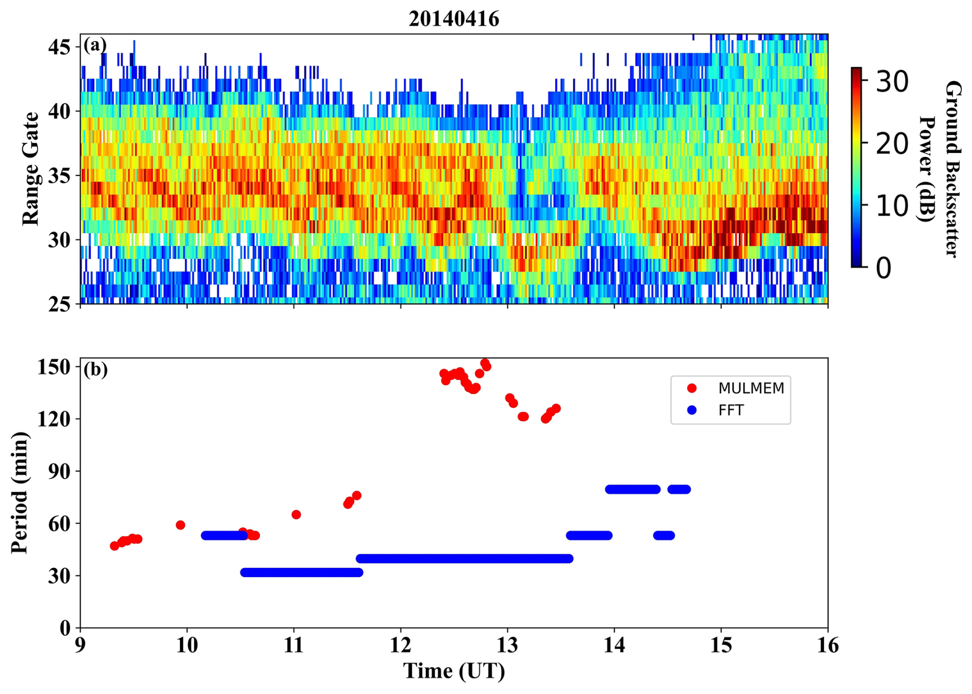
Figure 9 (a) RT plot shows an example of the MSTIDs. (b) Period of the observed MSTID derived using MULMEM (red curve) and FFT (blue curve).

4.2 Comparison of MULMEM & FFT results: A need for multi-instrument and multi-method studies

As explained above, the MULMEM analysis does not always return a result, so we have also computed the MSTID periods using FFT. We have compared the period of the observed MSTIDs from both methods and found some discrepancies, as seen in two cases with differing results as presented in Figs. 3 and 9. The period of the MSTID determined using the two methods in Fig. 3 are nearly the same, whereas the period determined in the second case (see Fig. 9) is different between 12:00 and 14:00 UT. Figure 9a (RT plot) implies that the time separation of the MSTID bands in this case was less than 60 min between 09:00 and 13:00 UT with a higher time separation (∼90 min) between 13:00 and 15:00 UT. This is consistent with the period determined using FFT (see blue curve in Fig. 9b). The period determined using the MULMEM (see red curve in Fig. 9b) is more than 120 min. We can infer from these results that MULMEM overestimated the period in this case. This might be due to the approach used by MULMEM. In MULMEM there is automatic selection of the time series, which could result in certain selections where MSTID structure was not prominent, and hence skipping of some MSTID bands. On the other hand, in the FFT method we have manually selected the time series where the MSTID bands were prominent in the RT plots to determine the period. To further investigate any disparity in the results, we have compared the average period of all the observed MSTIDs during the four years using both FFT and MULMEM, shown in Fig. 10. The red curve shows the average period determined using MULMEM and the blue shows the average period using FFT of each MSTID event. The period determined using both the methods generally shows quite similar values, however there are a few cases during 2009 and 2014 where MULMEM overestimated the period (Fig. 10c–d).

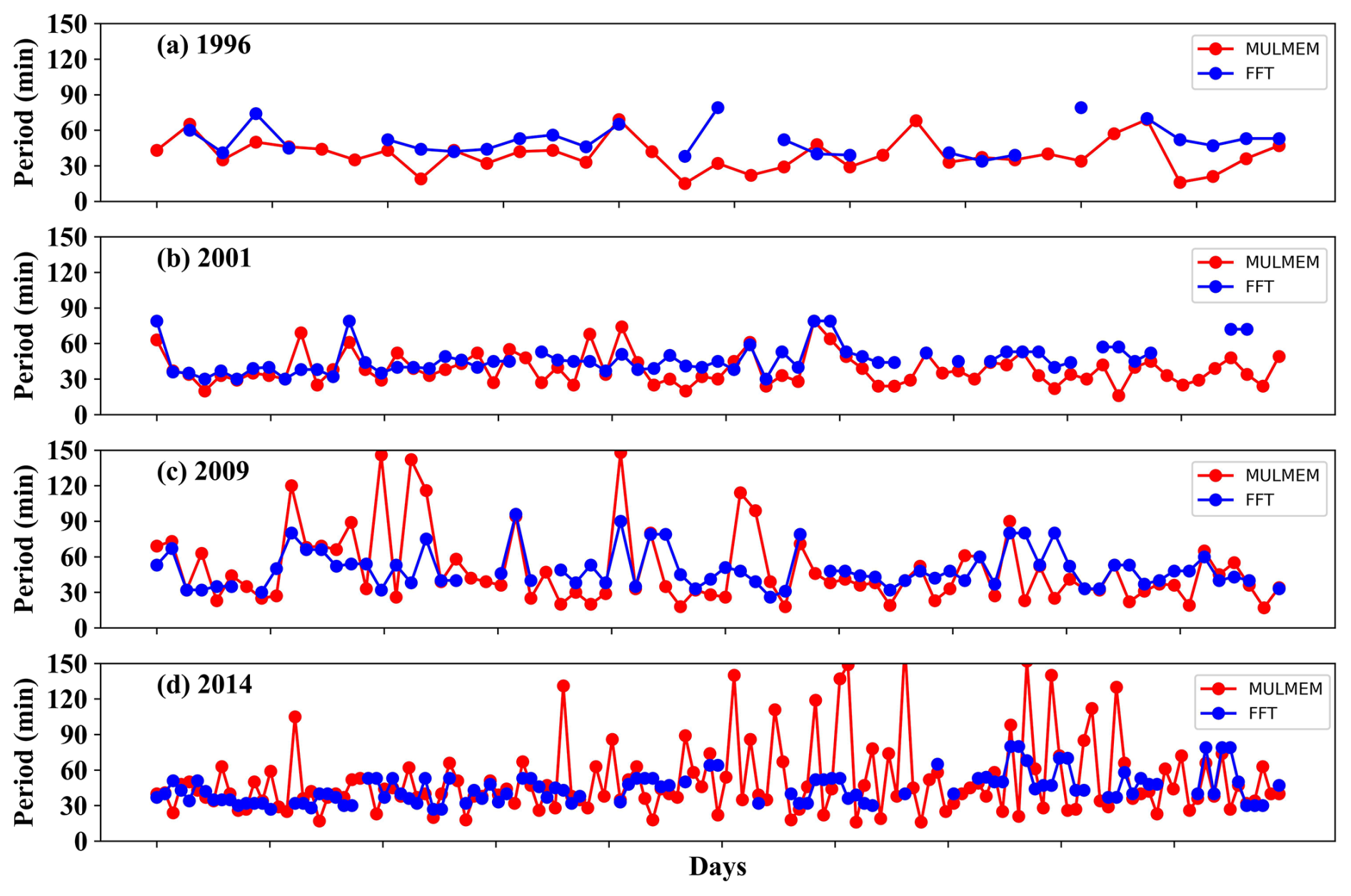
Figure 10 Shows the comparison of the period of MSTIDs (observed across all four years) derived using MULMEM (red curve) and FFT (blue curve) method.

These results assess the performance of MULMEM in the detection and parameter estimation of MSTIDs. The performance of MULMEM in detecting MSTIDs can be seen from Table 1 where the success rate of MULMEM hovered between 50 %–60 % with respect to MSTID events observed in RT plots. We have also assessed its performance in determining the MSTIDs' parameters. We find that MULMEM has estimated a similar period to the FFT (standard deviation <20 % of the mean period) in more than 75 % of cases. There are a few cases where it has underestimated/overestimated the period and in most of those cases the performance reduced due to weak (average GBS ≥15 dB) or noisy (continuous GBS between the MSTID bands) signals. It is also worth noting that the results in this study are based on a single dataset of GBS observations from the HAN radar, which itself shows a seasonal variation. Despite our efforts to account for the variation in GBS, it is nevertheless difficult to rule out the possibility that the seasonal variations and mischaracterization of the MSTIDs parameters might have some additional biases incurred due to observational constraints and inefficiency of the analytical method. Therefore, future studies will employ a multi-instrument and multi-method approach to mitigate any such biases in the observations.

5 Conclusions

This study has presented a statistical overview of high-latitude MSTIDs over the newly established EISCAT-3D radar site. To explore the characteristics and generating sources, ground backscatter data from the Hankasalmi radar during solar maximum (2001 & 2014) and minimum (1996 & 2009) years of solar cycles 23 and 24 have been used. The primary population of MSTIDs propagates equatorward with velocity and period in the range of 50–150 m s⁻¹ and 30–60 min, respectively. Their occurrence shows seasonal (primary peaks during winter and equinoctial months) as well as solar activity dependency (significantly higher occurrence (∼72 %) during solar maximum years). Furthermore, their occurrence shows little dependence on Kp index; irrespective of the Kp index conditions, it increases with increasing solar activity. It is interesting to note that MSTIDs show a comparatively high occurrence during prolonged northward and southward IMF B_z conditions with more than 80 % during solar maximum years. This increment in the MSTIDs occurrence might be due to the enhanced Joule heating caused by magnetic reconnection, either at the low-latitude or lobe magnetopause, during these IMF B_z conditions. It is interesting to note that their parameters (velocity, azimuth, and period) do not show any significant variability with respect to seasons, Kp index, IMF B_z conditions, and solar activity. This study tries to elicit the role of different sources (solar activity, geomagnetic activity, IMF B_z) on the generation of high-latitude MSTIDs but there still exists uncertainty regarding the dominant drivers. Also, in the determination of the characteristics using the MULMEM method an inconsistency has been observed, which necessitates a future study using a multi-instrument and multi-method approach.