Subauroral contamination in POES/Metop TED channels

Particle measurements from the Polar Operational Environmental Satellites (POES) and the Meteorological Operational (Metop) satellite program, are widely used for various scientific applications. While most studies focus on the Medium Energy Proton and Electron Detector (MEPED), the low-energy (eV and keV) counterpart, the Total Energy Detector (TED), has received comparatively less attention. However, the recent rise in the altitudes considered in ionization and climate models has increased interest in low-energy particle measurements as inputs for atmospheric ionization models.

This study analyzes TED particle data (together with selected MEPED channels) from 2001 to 2025 and shows that the TED 0° proton channels, in particular, are contaminated by energetic electrons at L<6, with weaker contamination observed in other TED channels. In some cases, the contaminated fluxes exceed typical auroral flux levels. The affected regions were cross-validated using auroral UV emissions and occurrences of GNSS derived S4 index to rule out the possibility that the observed fluxes correspond to real particle precipitation.

As correction approach, we provide a simple Kp- and channel-dependent latitude boundary that may serve as preliminary cut-off criterion for the contaminated regions. In a more advanced step, we identified the contamination characteristics of each particle channel on each satellite. The outcome is a list of problematic channels that should be neglected and a correction method based on background counts for the other channels. The corrected fluxes are in good agreement with UV emissions and the method is available in the additional material.

1 Introduction

Accurate spaceborne particle measurements are essential for various scientific fields, particularly for modeling the atmospheric impact of precipitating particles. These impacts include direct ionization and the production of nitrogen oxides (NO_x) (Rusch et al., 1981) and hydroxyl (OH) (Solomon et al., 1981, 1983), which can lead to catalytic processes such as ozone depletion (Crutzen et al., 1975; Heath et al., 1977; McPeters and Jackman, 1985; Funke et al., 2011). In the case of TED protons, these effects are primarily confined to NO_x production in the lower thermosphere, between 130 and 150 km. Due to its link to ozone chemistry, particle precipitation may also influence the radiation budget and, consequently, atmospheric dynamics.

However, particle measurements are often biased by contamination from different energies or particle species, out-of-view contamination, electric charging, and detector degradation. For the POES/Metop MEPED instrument, these issues have been extensively discussed and quantified. For instance, MEPED electron channels are known to suffer from proton contamination (Evans and Greer, 2006), which has been addressed using correction methods that subtract the spectral contribution of interfering protons (Lam et al., 2010; Asikainen and Mursula, 2013; Peck et al., 2015; Nesse Tyssøy et al., 2016). Monte Carlo simulations have also been employed to model the theoretical MEPED detector response to various particle species and energies (Yando et al., 2011). These simulations indicate that MEPED proton detectors are affected by energetic electron contamination, with the strongest impact on channel P1, decreasing in higher-energy channels. Another result of Yando et al. (2011) is that the integral electron channels MEPED 0° e1, e2, and e3 (as well as their 90° equivalents) are differently sensitive to high-energy electrons. In consequence a construction of differential channels by subtracting channels does not completely remove the high energetic electron component (in particularly when subtracting e3). The MEPED electron channels might also be affected by contamination from low-energy protons (see Yando et al., 2011). Additionally, proton detector degradation, which becomes relevant after 2–3 years in orbit, has been quantified using orbit intersections of different satellites (Asikainen et al., 2012). MEPED detector degradation has also been quantified by (Asikainen and Mursula, 2011; Ødegaard et al., 2016; Sandanger et al., 2015).

In contrast, studies on the data quality of the POES/Metop TED instrument remain scarce. The instrument description (Green, 2013) acknowledges energetic protons from the South Atlantic Anomaly (SAA) and energetic electrons from the radiation belts as primary sources of TED background counts. A correction for TED energy flux based on background count measurements is proposed in Green (2013), yet contamination from energetic electrons appears to persist. For example, Søraas et al. (2018, Figs. 4 and 5) observed a daily modulation in TED observations of sub-20 keV electrons between 50 and 62° invariant latitude during the 17 March 2013 geomagnetic storm, which they attributed to the penetration of relativistic electrons. Even more problematic is that no dedicated contamination analysis or correction has been conducted for the various TED energy bands. Given the growing demand for accurate low-energy particle measurements to support high-altitude atmospheric precipitation studies (e.g., Wissing and Kallenrode, 2009), this study aims to address that gap.

High-energy particle populations known to induce contamination are typically found within the radiation belts. For over 50 years, Earth's radiation belts have been understood to consist of two distinct zones – an inner and an outer belt-separated by the slot region (van Allen, 1959, 1983). The inner radiation belt primarily contains electrons in the 100 keV range and energetic protons exceeding 100 MeV, which are trapped by relatively strong magnetic fields. This belt typically spans L=1.2 to L=2.5 and remains relatively stable during quiet geomagnetic conditions (e.g., Selesnick et al., 2014). However, strong geomagnetic storms can significantly alter the inner belt proton population (e.g., Selesnick et al., 2014), and in regions such as the SAA, the inner boundary can extend to very low altitudes, where its downward extent is ultimately constrained by atmospheric losses. The outer radiation belt, in contrast, consists of highly dynamic electron populations (0.1–10 MeV) modulated by geomagnetic activity (e.g., Baker et al., 2013) with its intensity peaking between L=3.5 and L=5.5. In 2013, observations from the Van Allen Probes revealed a long-lived relativistic electron storage ring – a third radiation belt – that persisted for four weeks (Baker et al., 2013).

Contamination within the radiation belts has been documented for the POES/Metop MEPED instrument. For instance, Andersson et al. (2014) reported elevated MEPED electron count rates in the SAA that did not correspond to mesospheric OH enhancements, suggesting proton contamination as the likely cause. Similarly, Evans et al. (2008) identified anomalous increases in the POES proton channel > 16 MeV at subauroral latitudes near the SAA, which they attributed to contamination from electrons > 3 MeV.

During our analysis of TED data from POES and Metop satellites for the period 2001–2025, we identified very high fluxes – primarily in the proton bands – at subauroral latitudes. To investigate this phenomenon, we compared TED data with high-energy electron fluxes, TED background counts, and atmospheric measurements. Our findings indicate strong contamination, most likely from highly relativistic electrons, affecting the TED bands.

The objectives of this study are twofold: (a) To establish a simple latitudinal cut-off to exclude the contamination-dominated region, thereby enabling the safe application of TED data. (b) To develop a contamination correction method that can be applied to average TED fluxes, provided background counts are known, and that may also serve as an indicator of TED data quality in polar regions.

The structure of this paper is as follows:

Section 2 describes the data sets and processing methods. Section 3 presents the subauroral flux peak observations that motivated this investigation, along with their Kp dependence. Section 4 assesses the reliability of the measurements within the subauroral region. This section consists of four subsections: Sect. 4.1 provides an overview of the TED measurements. Section 4.2 explores energetic electron contamination as a potential cause of increased count rates at L=4. Section 4.3 examines the differing effects of contamination on TED species and orientations. Section 4.4 compares observed particle fluxes with independent data sets, demonstrating that TED proton channels do not capture real flux in the subauroral region. Section 5 quantifies the contamination effect for each channel, with Sect. 5.1 proposing a correction method based on TED background counts. In Sect. 5.2 the correction method is applied to measurements of year 2013. Section 6 summarizes our findings. The additional material contains the suggested correction method.

2 Data Sets

This section describes the data sets and data processing methods of this study. Section 2.1 introduces the data handling of the total energy detector (TED) particle measurements. After that the Modified Apex coordinate system is described, followed by the Kp-binning which has been applied to part of the paper's data base. In the next subsections two independent data sets are introduced, which are compared to the particle fluxes. These data sets are the backscattered UV, see Sect. 2.4 and the S4 scintillation index, see Sect. 2.5. The aim is to verify or refute particle precipitation in certain regions or during special periods with self-contained data.

2.1 Particle Data

The particle data originates from the Polar Operational Environmental Satellites (POES) and the Meteorological Operational satellite program (Metop). Both satellite series operate in sun-synchronous orbits at altitudes of approximately 820 km, with a revolution period of about 100 min and an inclination of approximately 98.5°. Although these satellites were initially placed in fixed local time orbits (morning-evening or day-night sector), their orbits have gradually drifted over time, enabling near-complete magnetic local time coverage (while combining multiple years and satellites). Even though we do not think that it notably impacts our results, the magnetic local time (MLT) coverage has a blind spot at 12:00 MLT limited to southern hemisphere subauroral latitudes and another at 00:00 MLT on the northern hemisphere. For details we refer to Fig. 1 (lower right) in Yakovchuk and Wissing (2019).

The particle detectors aboard POES and Metop are identical and integrated within the Space Environment Monitor SEM-2 (Evans and Greer, 2006). The SEM-2 comprises two instruments: the Total Energy Detector (TED) for low-energy particles and the Medium Energy Proton and Electron Detector (MEPED) for medium-energy particles. TED is a cylindrical electrostatic analyzer (a schematic of the TED configuration is shown in Green, 2013, their Fig. 1), while MEPED is a semiconductor detector with passive shielding.

This study focuses on the TED detector, which consists of a set of electrostatic analyzers (ESA). These analyzers utilize curved plates with predefined radii, modulated by different voltages, to allow only particles of specific energies to pass through and reach a channeltron (multiplier) at the end of the curved plates. TED features eight ESAs that differentiate between low and high energies, along with two inlet openings at 0° (zenith) and 30°. The detector mounting and it orientation in relation to the satellite is shown in Evans and Greer (Fig. 2.1.1 of 2004). Additionally, the curvature of the plates is oriented oppositely for protons and electrons. Particle flux measurements are conducted with the ESA plate voltage activated, while background counts are recorded with the voltage deactivated. Although this study primarily focuses on the upward-looking (0°) detector, which is crucial for observing precipitating particles at high latitudes, it also demonstrates that the TED 30° detector is similarly affected. It is important to note that at low latitudes near the magnetic equator, the 0° detector predominantly measures trapped particles (for the MEPED instrument this is shown in Fig. 1 of Rodger et al., 2010).

This study utilizes data from POES satellites N15, N16, N17, N18, and N19, as well as Metop satellites M01, M02 and M03. N16 is not used after 2006 as TED measurements are erroneous. In total the data covers the years 2001–2025. Details on the applied period and data averaging are given in the different sections.

Background counts are recorded but even though the TED data processing algorithm includes a background subtraction step (Green, 2013), this correction applies only to the total energy flux derived from a full energy sweep and not to individual bands. This holds true for both bin-format data prior to 2013 (Evans and Greer, 2004) and netCDF-format data after 2013 (Green, 2013). The differential TED bands are – until now – always provided uncorrected. The primary distinction between raw data and processed TED bands in the processed-data files is a multiplication by the geometric factor. Note that whenever we are mentioning the TED particles in this paper, we refer to these differential channels.

Since our study investigates the contamination of the total energy detector, a few words on the instrument's shielding are in order. Unfortunately the housing is not well documented, except for the total weight of the instrument, its dimensions and images showing the aperture. We will discuss this aspect when looking at the background counts. One important aspect is that the detector is stacked and that the inner instruments seem to be better shielded than the outer ones.

Data from the MEPED e3 channels have been used in order to identify high energetic electron fluxes. These data have been assigned an error value if high-energy protons, which can cause contamination, are detected. This filtering was performed on a 2 s basis using the high-energy P7 proton channel from the omni-directional detector as a proxy, with measurements set to an error value when counts exceeded 2 per second. Consequently, MEPED electron data is excluded during strong proton events and within the South Atlantic Anomaly. The energy ranges for all particle channels are detailed in Table 1. The channel names may be abbreviated, e.g. TED 0° proton band 11 as TED 0° p 11.

2.2 Coordinate System

This study employs the family of Magnetic Apex Coordinates (Van Zandt et al., 1972), which are derived from the International Geomagnetic Reference Field (IGRF) (Thébault et al., 2015). A key advantage of IGRF-based coordinate systems is that they account for the gradual movement of the geomagnetic poles, ensuring consistency in precipitation feature localization over extended time periods. This stability allows for multi-year spatial approximations of precipitation fluxes and facilitates the application of results to future datasets.

For ground-based locations and higher latitudes, Magnetic Apex Coordinates closely resemble the widely used Altitude Adjustment Corrected Geomagnetic (AACGM) coordinates. Specifically, poleward of 50°, the two systems are nearly identical (see Fig. 7 in Laundal and Richmond, 2017).

However, for positions above the ground, Magnetic Apex Coordinates provide a more accurate framework for describing charged particle behavior. These coordinates track the magnetic field lines from their footpoints upward, ensuring that charged particles remain on the same coordinates during their bounce motion. Thus, in Magnetic Apex Coordinates, the altitude of a satellite measurement does not alter the perceived location of a particle.

By default, the reference altitude for magnetic field-line footpoints is set to ground level. However, the Modified Apex Coordinates (Richmond, 1995) enable customization of the reference altitude. In this study, we use a reference altitude of 110 km, approximately where atmospheric interactions begin to dominate over magnetic field influences. Considering the grid resolution used, the effect of the reference altitude is negligible. Consequently, the coordinate system utilized is termed “Modified Apex 110 km Coordinates”, though we may refer to it simply as “APEX” in the text.

The conversion to Apex coordinates is done with an own C++ translation of the apex.f90 Fortran code as published on https://github.com/NCAR/apex_fortran/blob/master/apex.f90 (last access: 30 March 2026).

2.3 Kp-Binning of Particle Data

The planetary K-index (Kp) (Bartels et al., 1939) quantifies geomagnetic activity using a 3-hourly quasi-logarithmic scale ranging from 0 to 9. It is derived from observations at 13 geomagnetic observatories located between 44 and 60° in both northern and southern geomagnetic latitudes. The Kp index is sensitive to multiple current systems, including the ring current, and thus provides a global measure of magnetospheric activity.

For this study, particle data has been categorized into seven Kp-level groups: 0–0.7, 1–1.7, 2–2.7, 3–3.7, 4–4.7, 5–5.7, and 6–9. This binning approach enables the examination of particle flux variations as a function of geomagnetic activity.

2.4 SSUSI Data Set

We use the electron energy flux data from the Special Sensor Ultraviolet Spectrographic Imager (SSUSI) instruments on board the Defense Meteorological Satellite Program (DMSP) Block-5D3 satellites F17 and F18 (Paxton et al., 1992, 2017, 2018). These satellites fly at 850 km altitude in polar, sun-synchronous orbits, the equator crossing times of their ascending nodes are 17:34 LT (F17) and 20:00 LT (F18). The SSUSI detectors provide about 3000 km-wide spectrographic images of the auroral zones with a 10 km × 10 km pixel size at the nadir point. Of these spectra 5 UV channels are downlinked, including two colours for the LBH (Lyman-Birge-Hopfield) band emissions of N₂. From these two LBH colours the electron energies and energy fluxes are derived based on Strickland et al. (1983), additional discussion can be found in Knight et al. (2018). The electron energy flux data used here are provided within the Auroral-EDR (Environmental Data Record) data set at https://ssusi.jhuapl.edu/data_products (last access: 21 September 2020, no longer available online; SSUSI, 2020). The data files contain the data point locations in geomagnetic latitude and longitude in AACGM coordinates.

The data have been validated previously by comparing them to EISCAT ground-based observations (Bender et al., 2021). For the comparison here, for each DMSP/SSUSI orbit during 2013, the data points within 60° E ± 4° geomagnetic longitude were selected. The electron energy fluxes within these sectors were then averaged in one-degree latitude bins to produce the time series as shown later in Sect. 4.4.2.

It should be mentioned that the SSUSI-derived fluxes are based on the hypothesis that the UV-aurora originates from a pure electron spectrum. There is an on-going discussion how pure proton or mixed auroral spectra would show up in the results of these pure-electron calculations. While model calculations of Knight et al. (2012, their Table 4) and Gelinas and Hecht (2016) agree that this retrival technique should slightly over-estimate the atmospheric peak electron density under proton precipitation conditions, Knight (2021) did not see such an overestimation comparing SSUSI-derived atmospheric electron density with ionosonde observations. Concerning our paper we may summarize that – even though the SSUSI algorithms handle all UV lines as effect of electron precipitation – particle precipitation from both, electrons and protons, should show up in the SSUSI data set.

2.5 S4 Index

The S4 index is a standard measure used to quantify ionospheric scintillation, referring to rapid fluctuations in the amplitude and phase of radio signals as they pass through irregularities in the ionosphere. It is defined as the ratio of the standard deviation of signal intensity to the average signal intensity (Wu, 2020). For this study, we used S4 index values calculated from the signal-to-noise ratio (SNR) of GNSS radio occultation profiles. The S4 values, and thus the degree of disturbance of the profiles, refer to the altitude range of approximately 80 to 130 km above the Earth's surface. We analyzed the atmPhs or conPhs data product provided by UCAR for nine different satellite missions (CHAMP, GRACE, Formosat-3/COSMIC-1, PAZ, Spire, TerraSAR-X, TanDEM-X, KompSat-5, Metop-B, Metop-C, and PlanetiQ) measured within the latitude belt between 55 and 65° S from 2001 to 2024. Further, we concentrated on night-time measurements.

In total, 231 680 radio occultation profiles met our criteria. Using the method described by Arras and Wickert (2018), we calculated the maximum S4 index for each profile. Profiles that included a sporadic E signature were excluded from further analysis.

3 Observation of High Particle Fluxes in the Subauroral Zone

A distinct local maximum in TED proton flux, separate from both auroral precipitation and the South Atlantic Anomaly (SAA), was previously reported by Yakovchuk and Wissing (2019). This section examines which channels exhibit enhanced subauroral particle flux and how it correlates with geomagnetic activity.

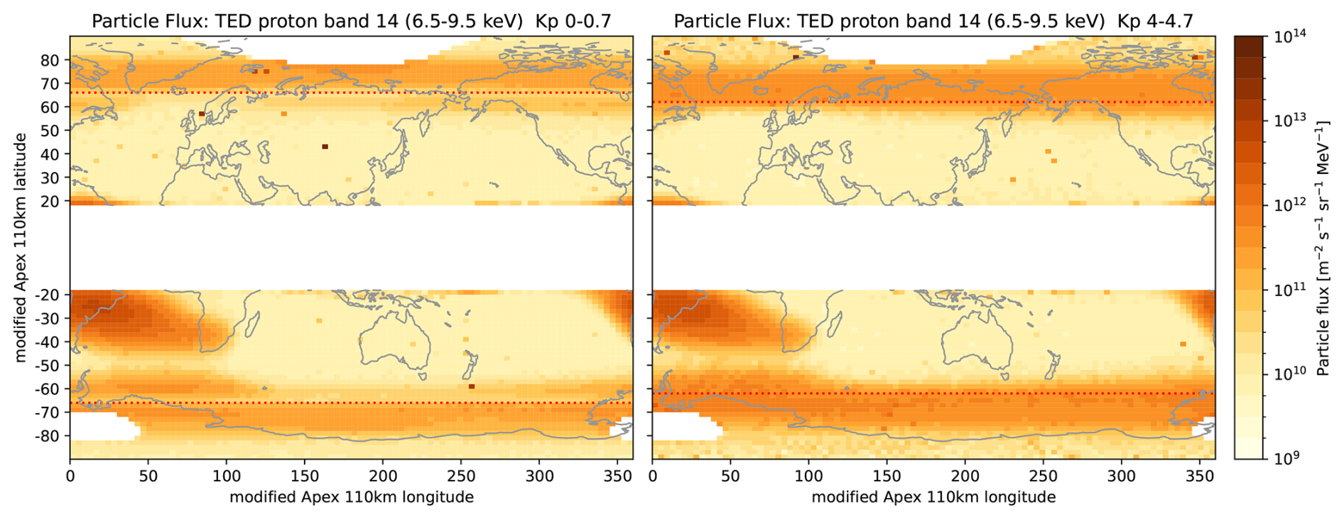
Figure 1 Spatial flux distribution of TED 0° proton band 14 for selected Kp levels (low Kp: left, medium Kp: right) averaged over the years 2001–2025.

Figure 1 presents the multi-year averaged spatial distribution of TED proton flux for the period 2001–2025, separated by geomagnetic activity levels (left: Kp = 0–0.7, right: Kp = 4–4.7). A localized increase in flux appears around 60° North and South APEX, with a stronger presence at longitudes that also intersect the SAA (most notably near 60° E APEX in the Southern Hemisphere).

At low Kp levels (Fig. 1, left), the flux distribution of all TED 0° proton channels exhibits a clear separation between the auroral oval and the subauroral peak, as indicated by the red dotted line. However, as geomagnetic activity increases (Fig. 1, right), the separation diminishes, with the auroral flux extending equatorward and merging with the subauroral peak. For Kp levels of 5 and above, the subauroral feature becomes indistinguishable from the auroral precipitation.

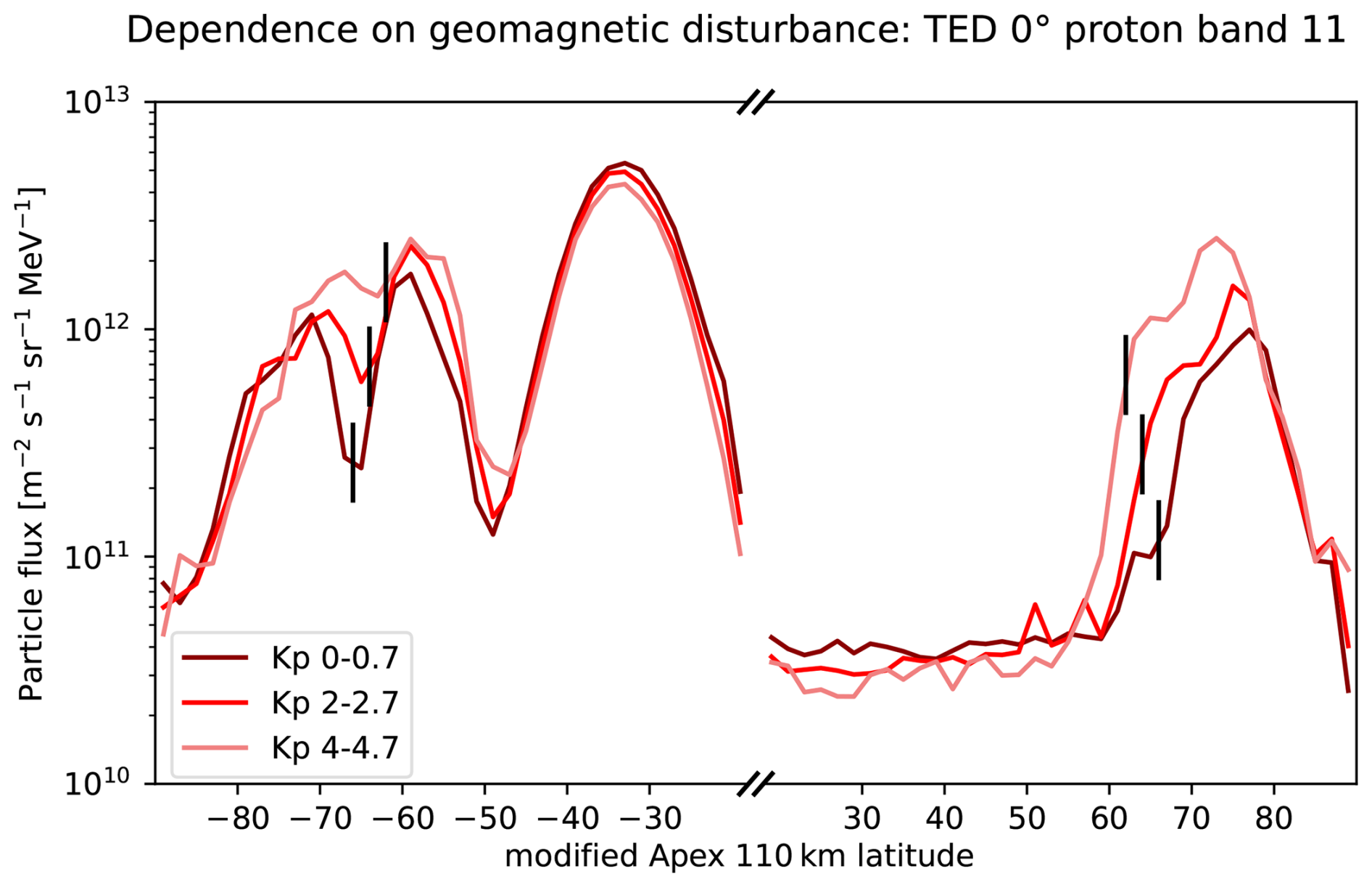
Figure 2 Cross-section at 60° E APEX for TED 0° proton band 11 during varying levels of geomagnetic disturbance (based on years 2001–2025). The vertical lines indicate the minimum between the auroral and subauroral peaks. Note that the latitude axis is stitched together, as modified APEX latitudes at 110 km altitude are constrained to values greater than 18°.

Figure 3 The subauroral peak of the TED channels cannot be adequately corrected based on scaled background counts. Either it creates strong negative fluxes around the peak or the correction does not noteworthy change the fluxes.

The dependence of the subauroral peak on geomagnetic disturbance is further illustrated in Fig. 2, which shows cross-sections of TED 0° proton band 11 at 60° E APEX for different Kp levels. While the subauroral peak consistently appears between 56 and 60° APEX in both hemispheres, increasing geomagnetic activity broadens and intensifies the auroral oval, shifting its equatorial boundary closer to the subauroral feature. As a result, the two regions may merge at moderate Kp levels (e.g., Kp = 4–4.7 in Fig. 1, right, for TED 0° proton band 14). However, differences in latitudinal extent and flux intensity suggest that portions of the subauroral peak remain distinguishable at moderate Kp levels. At higher Kp values, the subauroral peak becomes fully embedded within the auroral precipitation, limiting its identification to periods of low geomagnetic disturbance.

It is worth noting that the northern subauroral peak is generally weaker than its southern counterpart and 60° E APEX does not intersect its strongest region. An hemispheric asymmetry similar to this is typically seen in radiation belt populations measured on the same altitude because the polar horns of the radiation belt reach lower altitudes in the southern hemisphere due to the weaker magnetic field strength. The different radiation belt particle fluxes are shown e.g. in Winant et al. (2023) who compare the van Allen probe measurements on POES/Metop altitudes against the AE-8 model (Vette and Goddard Space Flight Center, 1991).

Figure 3 shows the flux of a TED proton band against L-shell. We also added scaled background counts, with the scaling factor chosen large as possible but still preventing unphysical negative counts at L=2–3 and L=6. The peak at L=4 remains largely unchanged, indicating that a simple linear background correction cannot eliminate the subauroral maximum without compromising physical consistency. This suggests that the background-corrected total energy flux may exhibit similar issues, as seen in Søraas et al. (2018, their Figs. 4 and 5).

Table 1 Channel and Kp combinations that exhibit enhanced subauroral flux, along with the location of the minimum between auroral and subauroral peaks, as identified visually from spatial maps such as Fig. 1. The latitude values apply to both the Northern and Southern Hemispheres.

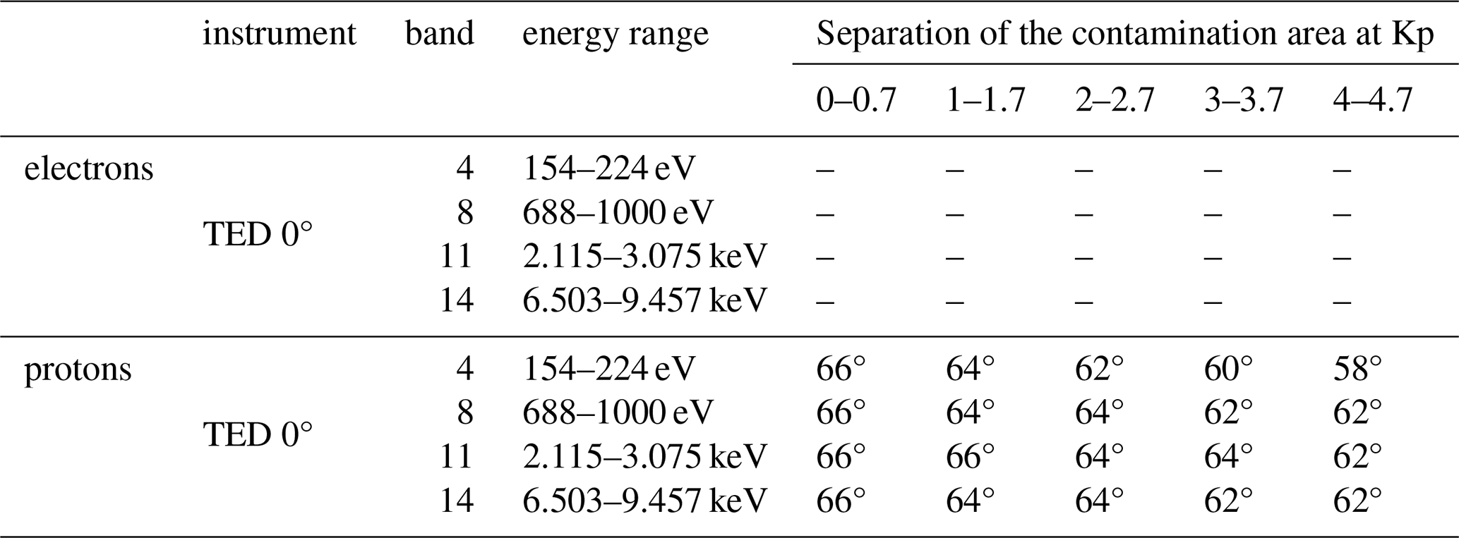
Table 1 summarizes the TED 0° proton channels and Kp conditions under which enhanced subauroral fluxes were detected. The identification criterion required the presence of a local flux maximum exceeding the equatorial boundary of the auroral oval by a factor of at least 1.778 (equivalent to one-quarter of an order of magnitude in logarithmic flux levels) across different longitudes, ruling out statistical fluctuations. Enhanced subauroral flux is observed across all TED 0° proton channels, whereas no corresponding feature is detected in TED electron data.

To illustrate the potential impact of a misinterpreted subauroral peak, we estimate its contribution to atmospheric ionization. Wissing and Kallenrode (2009, see their Fig. 9, lower panel) reported that at 120 km altitude, auroral proton-induced ionization accounts for approximately 14 % of total ionization, with electrons dominating the remaining contribution. If the observed subauroral TED flux is real, it would imply an additional ionization peak at this auroral proton level in the lower thermosphere (130–150 km). This highlights the importance of accurately characterizing the subauroral peak to refine atmospheric chemistry models.

4 Is the Subauroral Peak a Real Flux or an Artifact from Contamination?

A critical question regarding the observed subauroral particle fluxes is the reliability of the measurements. As noted in the introduction, high particle fluxes are expected at low L-shells, particularly in the proton and electron radiation belts. Two primary hypotheses can explain the subauroral peak: (a) The low-energy proton fluxes could represent a low-energy tail of the radiation belts. (b) The observed fluxes result from contaminated detector counts due to high-energy proton or electron contamination.

To investigate this, we analyze various particle measurements from the SEM-2 instrument.

4.1 Comparison of Onboard Particle Data

Figure 4 presents the mean particle fluxes recorded by the TED 0° detectors (left panels) and the TED 30° detectors (right panels) for the year 2013 under geomagnetically quiet conditions (Kp ≤ 0.7). The data are plotted against L-shell along two APEX longitudes: 60 and 160° E. Below L=6, the upper boundaries of each color correspond to 60° E APEX, while the lower boundaries correspond to 160° E APEX. The year 2013 was chosen because NOAA's data format update allowed easy export of TED background sensor counts per second (CPS). The figure also shows the MEPED e3 fluxes from the 0 or 90° instrument as indication for energetic electrons.

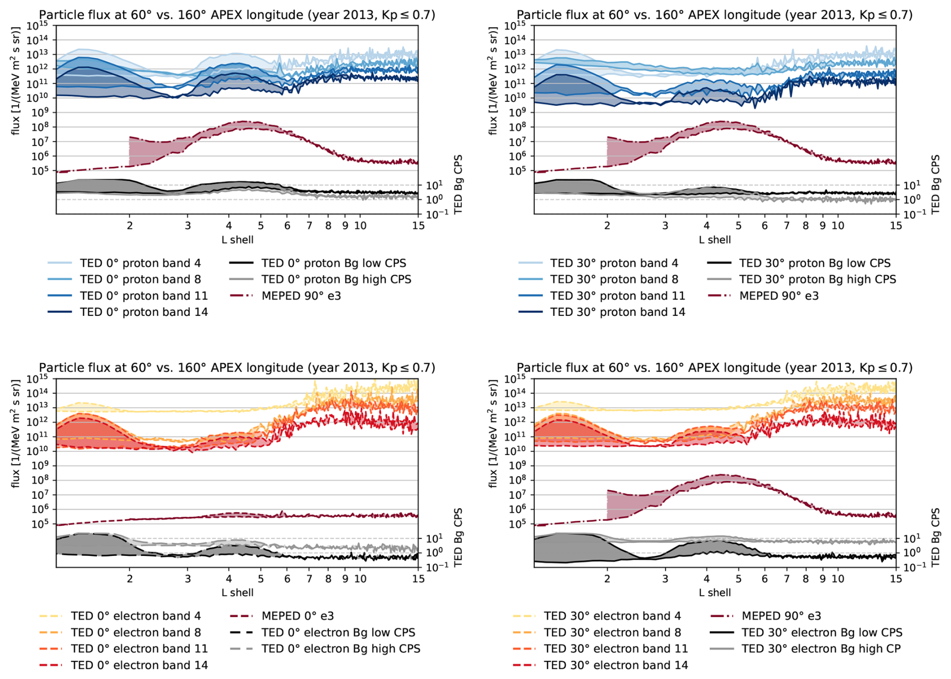
Figure 4 Particle fluxes and background sensor counts for the TED 0° (left panels) and the TED 30° detectors (right panels) in addition to the MEPED 0° or 90° e3 channel. The difference between 60 and 160° E APEX is highlighted by the shaded area. Below L=6, the higher counts (or fluxes) consistently correspond to 60° E APEX longitude, while the lower values correspond to 160° E APEX. Elevated background counts in the L≤2 (SAA) region and in the L=3–6 range (subauroral peak) coincide with intense particle counts in TED proton channels and the MEPED 90° e3 channel.

4.1.1 General Trends in the Data

Nearly all TED channels exhibit two local maxima: a) A peak at L≤2, associated with the South Atlantic Anomaly (SAA). b) A peak in the subauroral region (L = 3–6), with a maximum at L≈4 (∼60° N/S). This pattern is also reflected in the TED background counts (black for lower energy bands 1–8 and gray for higher energy bands 9–16).

4.1.2 The SAA and the Absence of Energetic Protons in the Subauroral Region

The SAA is well known for intense proton contamination, particularly affecting MEPED electron channels (Peck et al., 2015). Therefore we applied a filtering method for the MEPED electron channels, which uses the P6 channel to effectively remove heavily contaminated MEPED electron data from the SAA (L≤2). Indeed, all MEPED electron data of 60° E longitudinal cross section within the in the SAA are neglected.

However, the subauroral data remain unaffected by P6 filtering, which suggests that energetic protons are not responsible for the observed peak. This leaves two possible explanations: (a) The TED proton fluxes represent a low-energy tail of the radiation belt. (b) The measurements are contaminated by energetic electrons.

4.1.3 TED 0° Proton Fluxes

To gain further insight, we examine the flux characteristics in the subauroral region, starting with the 0° differential proton channels (Fig. 4, top left). All TED 0° proton channels exhibit a local maximum at L=4. The flux difference between 60° E APEX (peak) and 160° E APEX (minimum) roughly spans one order of magnitude across all TED 0° channels, albeit from different baseline levels. In contrast, background counts vary by only half an order of magnitude.

Notably, the shape of the background counts differs from the flux peaks. The background counts of TED 0° proton bands form a nearly plateau-like distribution, whereas the measured fluxes show a distinct peak at L=4. If the subauroral peak were purely due to contamination, a simple correction by subtracting background counts (even with a scaling factor) would not effectively remove the contamination.

4.1.4 TED 30° Proton Fluxes

A slightly different pattern emerges in the TED 30° proton channels (Fig. 4, top right). Here, the background count peak (as well as the flux) is lower than in the 0° channels. Additionally, the longitudinal variation (60° E vs. 160° E APEX) is less pronounced in lower-energy TED channels than in higher-energy ones. Interestingly, the expected subauroral peak in TED 30° proton band 8 is not clearly observed at L=4, despite noticeable longitudinal differences.

4.1.5 TED 0° Electron Fluxes

The 0° electron fluxes (Fig. 4, bottom left) exhibit the smallest subauroral peaks among all detectors. In TED 0° electron band 4, the peak is absent, likely due to naturally high count rates that mitigate contamination. In TED 0° electron band 8, a weak subauroral peak is visible only when comparing 60° E and 160° E APEX. The higher-energy electron channels (TED 0° electron band 11 and 14) do show a subauroral peak, but it remains one to two orders of magnitude below auroral flux levels.

4.1.6 TED 30° Electron Fluxes

For the 30° electrons (Fig. 4, bottom right), background counts in the subauroral region are higher than for 0° electrons. TED 30° electron band 4 remains unaffected, whereas the other TED electron channels show similar 60–160° E differences, with subauroral peak fluxes surpassing the 0° case.

4.1.7 MEPED 0 and 90° e3 Fluxes

The MEPED electron instrument is known to have contamination issues. Thus at first we should asses if this is relevant in our context. According to Pettit et al. (Fig. 6 in 2019) the corrected MEPED 0° e3 flux at L=4–6 may be factor 2 smaller than the uncorrected flux. A similar correction approach including both viewing directions was done by Asikainen and Mursula (2013). Their Fig. 5 (left) also shows a factor 2 for strong contamination events (note that their graph shows the reciprocal value). Considering the corrected 90° equivalent Asikainen and Mursula (2013)[their Fig. 5, right] gives a factor 1.2 to 1.45 more than the uncorrected flux. The impact of a factor 1.2–1.45 on Fig. 4 (as well as on Fig. 7, which follows in Sect. 5) is practically neglegible.

As indicated by MEPED 0° e3 (see Fig. 4, bottom left), the subauroral peak represents a local maximum in energetic electrons. But these fluxes are significantly substantially smaller than MEPED 90° e3 (see other panels of Fig. 4). The latter shows relatively small fluxes in the polar region and a dominant subauroral peak between L=4 and L=5 (note that data in the SAA is mostly removed). Within the subauroral area (which – in geographic coordinates – stretches from approx. 300° E, 70° S to 40° E, 55° S, see Fig. 1, top left, in Yakovchuk and Wissing, 2019) the MEPED 90° detector measures trapped, drift loss cone and bounce loss cone particles (compare Fig. 1, middle panel, in Crack et al., 2025). As the trapped population typically exceeds the other populations, we may simplify that averaged MEPED 90° fluxes in the subauroral area are mostly representing the trapped population.

The shielding of the MEPED detector housing should eliminate out-of-view electron contamination only up to about 6 MeV (Evans and Greer, 2006). Selesnick et al. (2020) showed that especially during periods of low pitch angle diffusion (most often occurring under low Kp conditions), most of the detector counts at L=4 in the 0° detector result from trapped or quasi-trapped (out-of-nominal field-of-view) electrons.

4.2 What might be the Reason for increased Subauroral Background Counts?

Energetic protons have already been excluded (see Sect. 4.1), but according to Li et al. (2001); Baker et al. (2013, 2019), highly relativistic electrons are common at L=4 as this region belongs to the outer (electron) radiation belt. Additionally, the so-called impenetrable boundary of >1 MeV electrons at about L=2.8 (Baker et al., 2014) fits to the background minimum seen in Fig. 4.

Energetic electron contamination can also explain the Kp dependence. On one hand there is the Dst-effect (McIlwain, 1966) which describes the outward radial motion of electron drift paths during increased geomagnetic activity in order to obey the third adiabatic invariant when the magnetic field strength drops. This is also connected with a reduction of electron energy. The Dst-effect itself in not connected to electron loss, it just temporarely displaces the electron populations, but particles may get lost to the interplanetary medium if their guiding field-lines cross the magnetopause (e.g. Kim et al., 2010). Loss processes are typically observed during high geomagnetic activity. Iles et al. (2002) states significant losses during storm main phase that may remove the majority of trapped electrons while conditions of recovery determine if there is an increase or decrease afterwards. Millan and Thorne (2007) provide a review summarizing loss processes and the connected wave activity during different geomagnetic activity. Further evidence is provided by a case study from Turner et al. (2012) showing that the radiation belt electron flux drops by orders of magnitude during geomagnetic storms. A quick radiation belt recovery, which was also noted by Turner et al. (2012), or increased radiation belt electrons fluxes after 53 % of the investigated geomagnetic storms as observed by Reeves et al. (2003) do not contradict this statement as the increased fluxes are observed after the main event and thus during lower Kp-values (or Dst-values, as seen in Fig. 2 of Reeves et al., 2003). The same is shown in Ross et al. (2021). Their Fig. 14 compares 4.2 MeV radiation belt electron measurements of the Van Allen Probes at different L-shells with Kp. Whenever the Kp rises to higher levels (say above 5), the electron flux decreases by orders of magnitude. This is most prominently seen at around L≈4 and can be used as indication for reduced contamination at higher Kp.

In the context of our study, it is unnecessary to distinguish between the Dst-effect displacements and loss processes such as magnetopause shadowing or atmospheric interactions, as all lead to a (at least short-term) reduction in energetic electron populations, thereby resulting in reduced contamination during periods of high geomagnetic activity.

Comparing the location of the background peak with MEPED 90° e3, we conclude that the contaminating electrons should have slightly higher center energy than MEPED 90° e3. Observations from Peck et al. (2015, see their Fig. 5) constructing a virtual electron channel e4 with a higher energy center of 800 keV (based on the MEPED P6 proton channel) show a flux maximum at L=4, similar to Ross et al. (2021) for 4.2 MeV electrons, which agrees to the observed background count peak.

To conclude this subsection, the abundance of high-energy electrons is most likely responsible for the TED background counts and suggests that contamination in the TED proton channels (and to some smaller extent in the TED electron channels) is occurring. However, due to the absence of a correction algorithm, this does not provide a direct measure of the actual abundance of low-energy particles. In other words, it remains unclear whether the contamination is strong enough to fully account for the observed peaks in the low-energy channels.

4.3 Why do not all TED Channels show the same Background Counts?

The background counts, as well as the channels' difference between 60 and 160° E APEX, are highest for TED 0° protons and TED 30° electrons, while TED 30° protons and TED 0° electrons show less impact. (Note that the different background levels are shown in Fig. 4 as well as in Fig. 8 where we are focussing on a single satellite).

The shielding of the TED instrument is unfortunately completely undocumented. Using very rough estimations on the volume, mass, and material, we end up with an eventual tungsten shielding of probably less than 0.8 mm, which would allow penetration of electrons >2 MeV according to the ESTAR database¹ from NIST. However, this is very vague. According to private communication with Juan Rodriguez (NOAA), it might be better to assess contamination candidates by coincidence.

This, however, does not explain any differences between the detectors. In fact, combining a TED detector image (see https://www.eoportal.org/satellite-missions/noaa-poes-series-5th-generation#sem-2-space-environment-monitor-2, last access: 30 March 2026) and the information on the size of the single detector openings, allowed us to determine the layout of the TED detector stack, being from side to side: 0° protons, 30° protons, 0° electrons, 30° electrons. Given that both inner detectors show fewer background counts, we conclude that this is an effect of better (lateral) shielding.

4.4 Comparison to Different Data Sets

The most relevant datasets for comparison are those from satellites with similar orbits. However, these datasets often suffer from the same issue – particle measurements in the radiation belts are problematic and frequently omitted. For instance, data from the METEOR-3M satellite program (accessible at https://ftp.sinp.msu.ru/meteor-3m/msgi/L1/ and http://smdc.sinp.msu.ru/, last access: 1 March 2021) are subject to such limitations.

Regarding different orbits, the TED data can be compared to the HOPE instrument onboard the Van Allen Probes. Yue et al. (2017, their Fig 2) shows statistical flux maps of low energetic 11 keV protons. During Kp ≤ 1 the highest fluxes are observed between L=5 and the image boundary at L=6. It steadily decreases till L=2 or 3 where it reaches the minimum flux. During higher Kp the flux is increased from the outher boundary down to L=4 while L=4 does not represent a local maximum. This is in contrast to the (contaminated) flux of the TED channels that show a maximum at L=4 (compare Fig. 4). However, it agrees with the SSUSI observations (discussed later in this Section) that show enhanced fluxes at L=4 (equivalent to −60° APEX) only during active periods. Higher proton energies of 55 keV from RBSP-A/RBSPICE as investigated by Li et al. (2023, their Fig. 1) show a similar pattern but are already relatively far from the TED energy range (<10 keV).

In this study we adopted a different comparison approach. If the peak observed in the low-energy 0° detectors is real, it should manifest as particle precipitation in the atmosphere at the footpoints of the corresponding magnetic field lines (which coincide in APEX coordinates). To assess the atmospheric impact, we applied two independent methods. First, we examined the S4 index: a peak in TED proton flux at TED energies should result in an ionization peak at approximately 150 km altitude, which should be reflected in the S4 index. Second, particle interactions in the upper atmosphere should produce UV radiation, which can be detected using auroral imagers such as SSUSI. The benefit of this comparison is that these measurements are independent of particle contamination issues.

4.4.1 Comparison to S4 Index

Figure 5 compares the S4 index (top panel), which serves as an indicator for ionization layer formation, with the particle flux from an affected TED channel, TED 0° proton band 11 (middle and bottom panels).

Figure 5 The top panel shows the GNSS-derived S4 index at 55–65° S, averaged over all available night-time (20–4 local time) profiles from 2001 to 2024 that do not exhibit a sporadic E-layer. The S4 index serves as an indicator of disturbances in the ionosphere. The middle panel presents the average particle flux in TED 0° proton band 11 for the same latitudinal band, covering the same years and the same filtering for night-time values only. The bottom panel condenses the middle panel’s data into a latitudinal mean, allowing for direct comparison with the S4 index.

The S4 profiles in the first panel have been restricted to night-time² (20:00–04:00 LT). The night-time S4 index is elevated between 80–190° E geographic longitude with a main peak at 100–120° E.

The second panel illustrates the particle flux for TED 0° proton band 11 without any Kp filtering for the same period and night-time selection as the S4 index data set. The sinusoidal shape originates from the auroral oval in geographic coordinates, reaching latitudes closest to the equator at 90–150° E geographic. The highest flux values (above 10¹² MeV⁻¹ s⁻¹ sr⁻¹ m⁻², yellow) occur between 320 and 50° E geographic, corresponding to subauroral latitudes in APEX coordinates. Note that the SAA itself is not shown here as it is located equatorward of 50° S. The lowest flux values appear between 250 and 300° E geographic, aligning with a region equatorward of the subauroral peak.

The bottom panel condenses the 2D information from the middle panel into a latitudinal mean, allowing direct comparison with the top panel. It shows three peaks, the highest one at 15° E which belongs to the subauroral TED flux but which does not appear at all in the S4 data. The other two TED maxima at 70° E and – even higher – at 170° E belong to the auroral oval. The peak at 170° E clearly appears in the S4 data whereas the 70° E maximum is part of the main auroral S4 maximum which also contains other energy channels and of course the electron precipitation. Lower-energy particles create an auroral pattern that extends further poleward, leading to a single peak.

Note that Fig. 5 is not very sensitive to high Kp particle precipitation. First, the temporal contribution is small and second all shown latitudes would be similarly affected, resulting in a mostly longitude-independent S4 offset.

The take-away message is, that in the region between 320 and 50° E geographic, where the TED channel registers a flux maximum, the S4 index does not indicate a corresponding ionization increase. Since particle precipitation at a specific energy should produce a distinct ionization and scintillation signature at a predictable altitude, the low S4 index suggests that the observed TED proton flux in this region is contamination from the horns of the outer radiation belt.

4.4.2 Comparison to SSUSI

The first 5 panels of Fig. 6 present the precipitating energy flux for the year 2013 based on different instruments. For better comparison all energy ranges have been matched to the SSUSI data set, which is limited to an upper energy of about 20 keV.

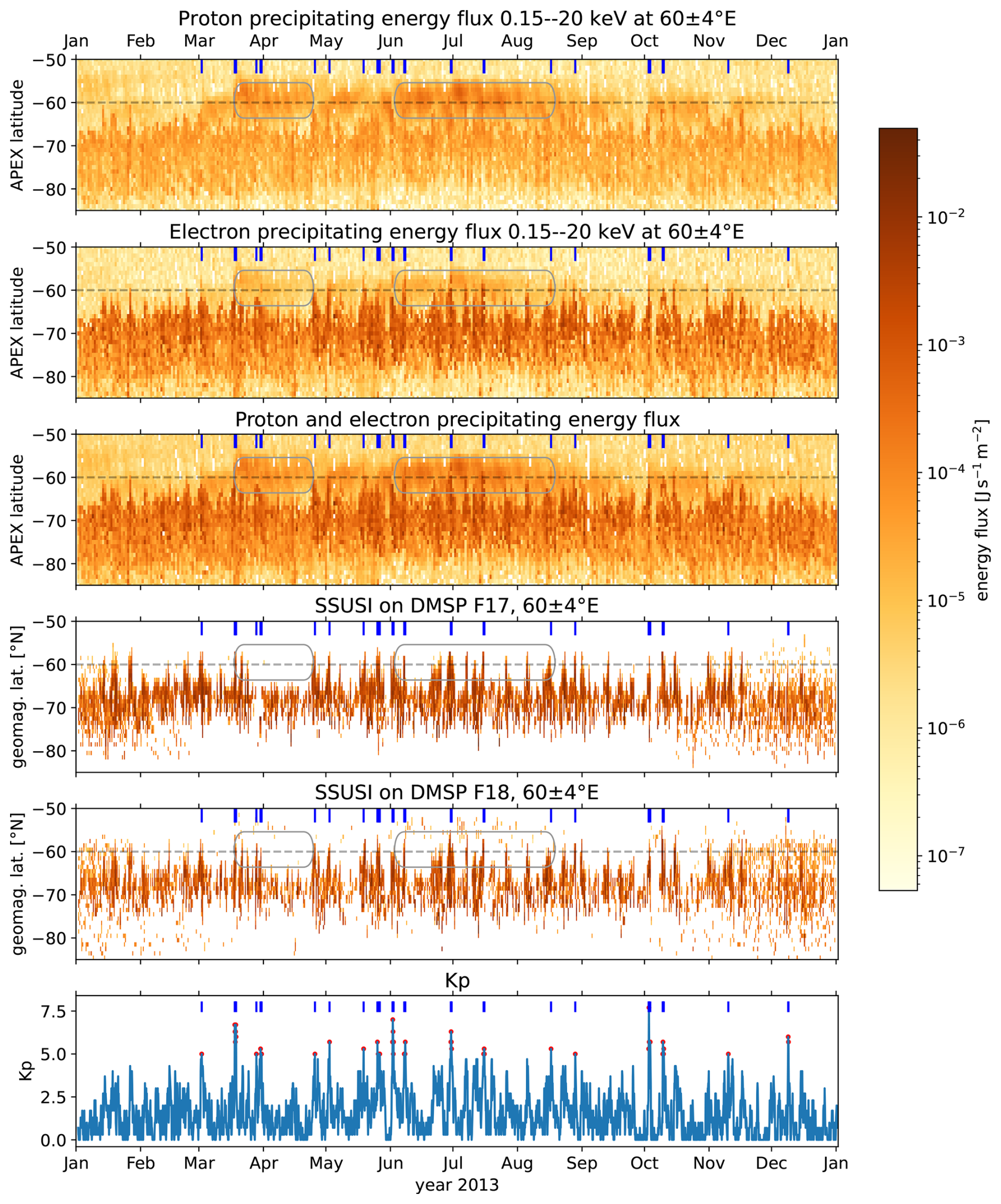
Figure 6 Temporal evolution of electron energy flux, proton energy flux, and their combined flux, compared to the energy flux derived from SSUSI auroral UV radiation as observed by two satellites, and the geomagnetic activity represented by Kp for the year 2013.

Figure 6 (top panel) presents the total precipitating proton energy flux derived from spectrum fits of all TED 0° proton channels and MEPED 0° P1. The highest TED channel already covers 6.5–9.5 keV thus MEPED 0° P1 is only used for the extrapolation up to 20 keV with very limited impact on the total precipitating flux. Two regions exhibit increased flux: one centered around 70° S APEX latitude, indicative of auroral precipitation, and another at 60° S APEX latitude, corresponding to the subauroral peak. Periods of Kp ≥ 5 are marked by blue lines in the upper part of the graph and also shown in the bottom panel. The subauroral peaks tend to follow periods of elevated Kp, and in some cases, the subauroral proton energy flux exceeds that of the auroral region. Two instances of strong subauroral peaks are highlighted for comparison.

The second panel displays the electron energy flux (154 eV to 20 keV) from the TED 0° electron channels and MEPED 0° e1–e2, a differential channel derived by subtracting e2 from e1. Based on results from Yando et al. (2011) this channel subtraction removes the impact of energetic electrons. As in the proton case the MEPED channel is used only from 9.5 keV to 20 keV in order to extrapolate the spectrum to the same energy range as the SSUSI data set.

Unlike the proton flux, the subauroral electron contribution is noticeably smaller, while the auroral electron flux is more pronounced. Additionally, auroral electron flux strongly depends on geomagnetic activity, intensifying and shifting equatorward during high Kp conditions. The proton flux exhibits similar behavior, albeit at lower intensities.

The third panel combines proton and electron energy fluxes. The subauroral contribution is comparable to auroral levels, underscoring the need to determine whether the subauroral flux is real or an artifact.

Panels 4 and 5 present UV-derived energy fluxes from auroral emissions measured by DMSP-17 and DMSP-18, respectively. Both datasets exhibit a strong Kp dependence, with increased energy flux during geomagnetic disturbances and auroral emissions extending to approximately 60° S APEX latitude. This aligns with the electron flux observations in the second panel. However, the marked subauroral peak does not appear in the UV data, even though the combined energy flux matches levels recognized as auroral emissions on some days. This suggests that the subauroral proton energy flux is overestimated.

Given the similarities in detector design, it is likely that the TED electron channels experience subauroral contamination as well. However, since the subauroral electron flux is lower, it may not be detectable in SSUSI data.

In summary, Figs. 5 and 6 independently demonstrate – through the absence of ionization effects and auroral emissions – that the subauroral peak does not correspond to real precipitating low-energy particles. The only times when precipitation effects are recorded in this region coincide with geomagnetic storms, during which the auroral oval expands into this latitude range (see Fig. 6, second panel).

It is worth noting that Kavanagh et al. (2018) observed particle precipitation events at L<4 (slot region) while comparing electron measurements exceeding 640 keV (potentially above 1 MeV) with riometer measurements. These slot region filling events persist long after the storms that generate them and exhibit low Kp dependence. However, our observation methods, which focus on the upper atmosphere, do not capture deep atmospheric ionization (occurring in the lower mesosphere to stratopause, 50–55 km altitude). This suggests that while an energetic electron population is often present at low Kp, contributing to deep atmospheric ionization and contamination, the majority of TED proton channel fluxes during these periods are likely artifacts.

It is important to mention that disproving the existence of a subauroral low-energy proton peak during low Kp does not invalidate the possibility of subauroral proton precipitation in general. Kim et al. (2021) linked low-energy subauroral proton precipitation to EMIC wave activity. However, their study focused on substorm periods without high fluxes of electrons exceeding 100 keV.

5 Estimation of Contamination

Figure 7 illustrates the correlation between TED 0° proton band 11 and MEPED 90° e3 throughout 2013. It reveals two distinct particle populations. At low MEPED 90° e3 flux levels (up to approximately 10⁸/(MeV s sr m²)), the TED 0° proton band 11 flux distribution remains largely independent of the electron flux. However, beyond this threshold, the peak fraction of the TED proton flux distribution (dark red area) increases with rising energetic electron flux. Notably, most data points in this second population originate from the subauroral region.

Figure 7 Correlation of TED 0° proton band 11 and MEPED 90° e3.

As demonstrated in Sect. 4, particularly in Sect. 4.4, the elevated TED fluxes in subauroral regions are not real. This strong correlation is a clear indication of contamination.

One might argue that the large difference in flux levels between these channels should prevent strong contamination; however, this is not the case. The secondary axis in Fig. 7 presents integral fluxes across the full bandwidth of each channel. Within the correlated population, the peak fraction of the TED proton flux distribution follows a roughly one-to-one relationship with MEPED 90° e3, albeit with considerable spread. Additionally, MEPED 90° e3 does not even peak at the same L-shell location, suggesting that a higher-energy electron channel – such as the virtual electron channel proposed by Peck et al. (2015) – might yield an even stronger correlation.

Another factor to consider is that both particle channels can record zero flux, indicating that the detectors' integration time may be insufficient to capture a meaningful flux level. Zeros in MEPED 90° e3 are binned separately (see the left subfigure in Fig. 7), while TED 0° proton band 11 registers zero flux at 16 s resolution in approximately 70 % of cases, with this fraction decreasing above 3×10⁷/(m² s sr MeV).

In conclusion, TED 0° proton band 11 – and likely other TED channels – should be treated with caution when MEPED 90° e3 flux level exceeds 10⁸/(m² s sr MeV). Due to the large spread in the data and the probably higher center-energy of the contaminating population, a simple subtraction of MEPED 90° e3 scaled by its bandwidth would yield unreliable results and is therefore not recommended.

5.1 Correction Based on TED Background Counts

A natural approach to correct TED bands involves a subtraction of background counts, as applied by Green (2013) for total energy flux. However, Fig. 4 (e.g., top left) and Fig. 3 highlight two key challenges: (1) a proper conversion of background counts to physical flux is required, and (2) the non-linear response during high contamination must be accounted for. The background peaks observed in the South Atlantic Anomaly (SAA) and the subauroral region flatten at high values, a behavior not seen in uncorrected TED flux or the contaminating MEPED 0° e3 peak. Consequently, applying only a simple linear scaling to match SSUSI observations at subauroral latitudes would introduce unphysical negative fluxes at L=2.5–3.

Different possible physical or technical sources of non-linearity come to mind. First, saturation effects may arise due to the longer integration time of the background detector (3.2 s) compared to 0.2 s for individual band measurements. However, the highest recorded background counts remain below 30 – far from the allowed maximum of 1 999 848 stated in Green (2013). Second, non-linearity could stem from data compression during satellite transmission (see Table 14 in Green, 2013). Yet, since we observe non-integer values, we trust that these represent decompressed counts (see Table 15 in Green, 2013, and notes in the netCDF files). Third, orbital motion during measurement could contribute: background counts are averaged over 16 instrument cycles (32 s total), during which the satellite travels about 270 km (or 1° latitude). This spatial averaging naturally smooths background peaks compared to individual band measurements. However, direct comparison with the old bin-format reveals that the saturation effect is caused by a different handling of the background data in the netCDF-files. In the netCDF-version all background data above an arbitrary level are cut and replaced by a linear interpolation of the closest surrounding background values. We probably can call this a bug as it unnecessarily hides the real (much higher) background values.

The underlying assumption for an empirical contamination correction is that a given background count level corresponds to a predictable level of contamination in the particle bands. Since multiple flux measurements exist for each background count level, the lowest observed flux should best approximate the contamination component. We thus use the dataset from Fig. 4 (without longitudinal restrictions and separately for each satellite as well as a similar data processing for M03 in year 2020, as it was not launchend in 2013, and the same for N16 in 2005, which was already defect in 2013) to estimate the lower flux envelope for each background count value.

Figure 8 TED channels of NOAA15 plotted against their individual background channel.

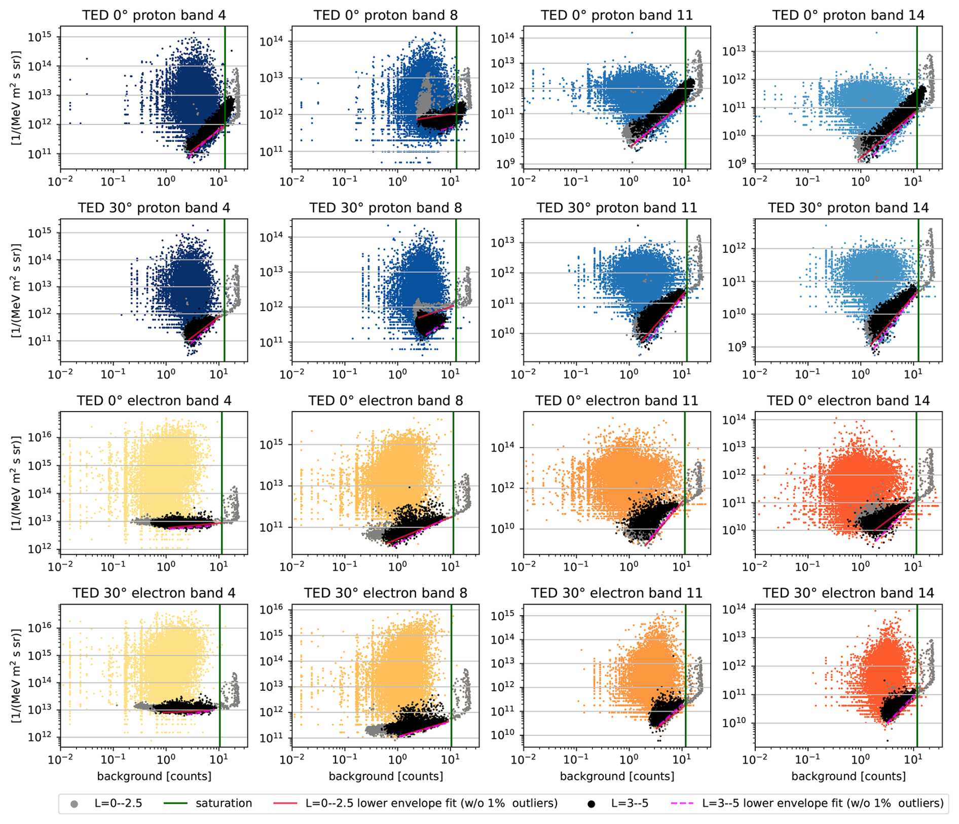
Figure 8 shows the particle populations at L=0–2.5 (grey, including the SAA), L=3–5 (black, subauroral area) and L>5 (colored) by plotting background counts against individual particle bands for NOAA15. Using TED 0° proton band 11 (top panel, third column) as typical example, the last group (in color, here blue) is centered around (10⁰, 3×10¹¹) and mostly represents uncontaminated flux (meaning that the flux may be orders of magnitude higher than the contamination). The first group (SAA, gray) forms a narrow band –on a wide range linear in log-log– extending to the highest background counts (about 2⋅10¹) where background channel reaches a (in this representation inverted) plateau, indicating the saturation-like cut-off. The second group (black) corresponds to the subauroral region (L=3–5) and shows the same dependency on background counts as the SAA population but does not reach the highest background counts. Also the flux variation for a specific background level is typically higher (except for TED 0°/30° p 8).

Notably, contamination effects appear more pronounced in the outside detectors (TED 0° p and 30° e). This can be seen clearly as the peak contamination within the subauroral population (gray) reaches much higher background values in 0° p than in 30° p (same in 30° e compared to 0° e). This relation is observed in all satellites and is generally more pronounced than in N15.

To estimate the lower contamination envelope we first need to define the boundaries. The upper boundary is the saturation threshold. The saturation effect was evident in practically all SAA distributions³. In order to estimate the saturation level, we binned the distribution (consisting of background count vs. particle flux pairs) into 20 logarithmically equidistant background levels, derived the standard deviation of the logarithmic particle flux within these bins and selected the highest increase of the standard deviation between neighboring bins as indication for the beginning saturation. The green vertical line (now called saturation threshold) marks the background value that corresponds to the boundary between these bins. In many cases the saturation threshold of 0 and 30° viewing angles were close to each other. Within each of the 20 logarithmically spaced background bins, the pairs were sorted by flux, and the logarithmic flux distance to the following pair is determined. In order to suppress outliers, 1 % of the data are omitted, depending on this distance. While this filtering would also remove isolated data points within the distribution it turned out to be effective in removing outliers below more populated areas. The pair with the lowest remaining flux value in each bin is returned and creates the data base for the lower contamination envelope fit. However, a contamination should positively correlate with the background counts. Therefore the minimum flux of all returned pairs is selected and its background count is used as lower boundary for the fit. The we applied a linear fit to the logarithmic background counts log ₁₀(b_g) and the logarithmic lower envelope channel flux log ₁₀(Φ_LE) in form of ${\log }_{\mathrm{10}}\left({\mathrm{\Phi }}_{\mathrm{LE}}\right)=a\cdot {\log }_{\mathrm{10}}\left(b_g\right)+b$. Fit parameters for the SAA (L=0–2.5) and subauroral region (L=3–5) are presented in Tables 2 and 3 and depicted in Figs. 8 (for N15), 9 (for problematic channels) and 10 (for all satellites).

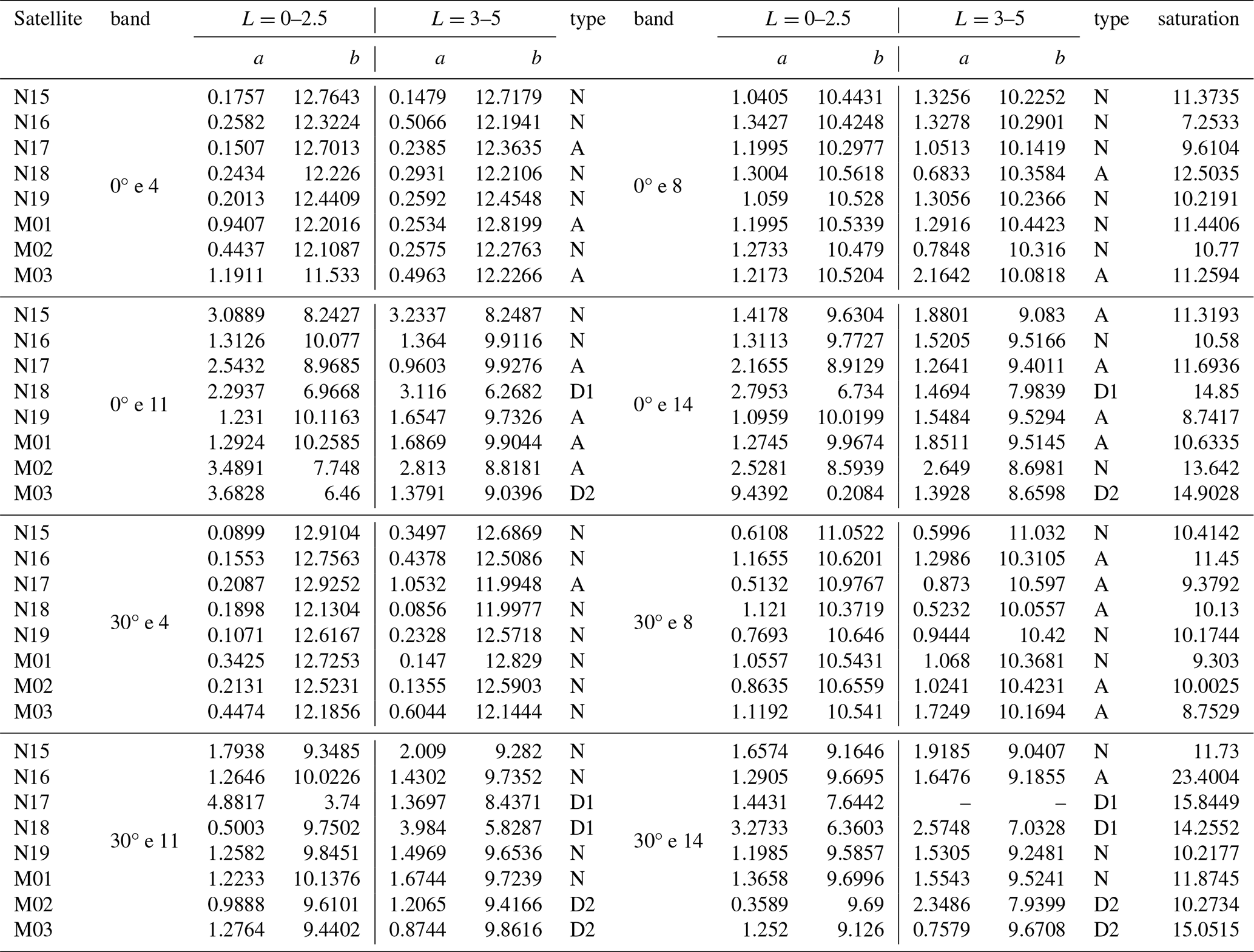
Table 2 Fit parameters of the lower envelope of the contamination and the saturation threshold for the proton bands. When applying the (averaged) background flux b_g to ${\log }_{\mathrm{10}}\left({\mathrm{\Phi }}_{\mathrm{LE}}\right)=a\cdot {\log }_{\mathrm{10}}\left(b_g\right)+b$ the resulting lower envelope flux Φ_LE is given in 1/(MeV m² s sr). The Table only states fits that may be used for a correction. “N” stands for “type normal”. Further information on the types is given in Fig. 9 and the related paragraph.

Table 3 Same as Table 2 for the electron bands.

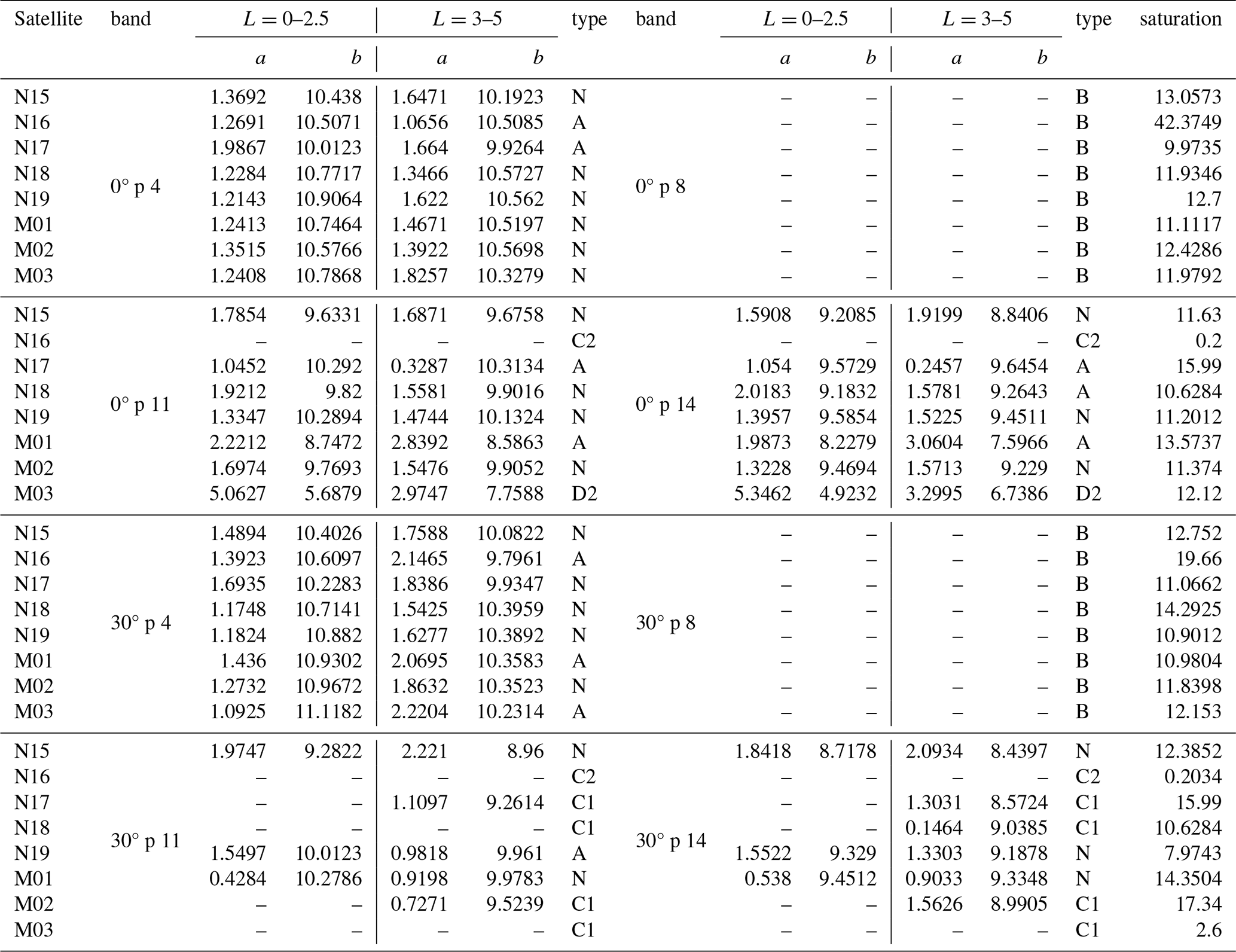
N15 (see Fig. 8) seems to have relatively good particle detectors. Meaning that within most channels the contamination is proportional to the background values (below the saturation threshold). Also the contamination seems to be similar within the SAA and the subauroral area. Given the main expected contamination sources being protons in the SAA and electrons in the subauroral area the contamination is independent of particle type. This is indicated by the matching reddish solid and dashed lines labled as lower envelope of the associated area. Also the saturation threshold is above typical values reached in the L>5 region, which means that (at least at these Kp values) a cut at the saturation threshold is not problematic. We will call this case “type normal”. As a correction attempt all values below the saturation threshold may be subtracted by typical background contamination which should be the lower envelope (a certain factor may take statistical variations into account). In case that the TED flux does not show a positive correlation with background counts we omit the fit and no background is subtracted. All data above the saturation threshold should be discarded. However, TED 0° proton band 8 shows that “type normal” does not apply to all channels.

Figure 9 Different types of problematic contaminaton (see text for details).

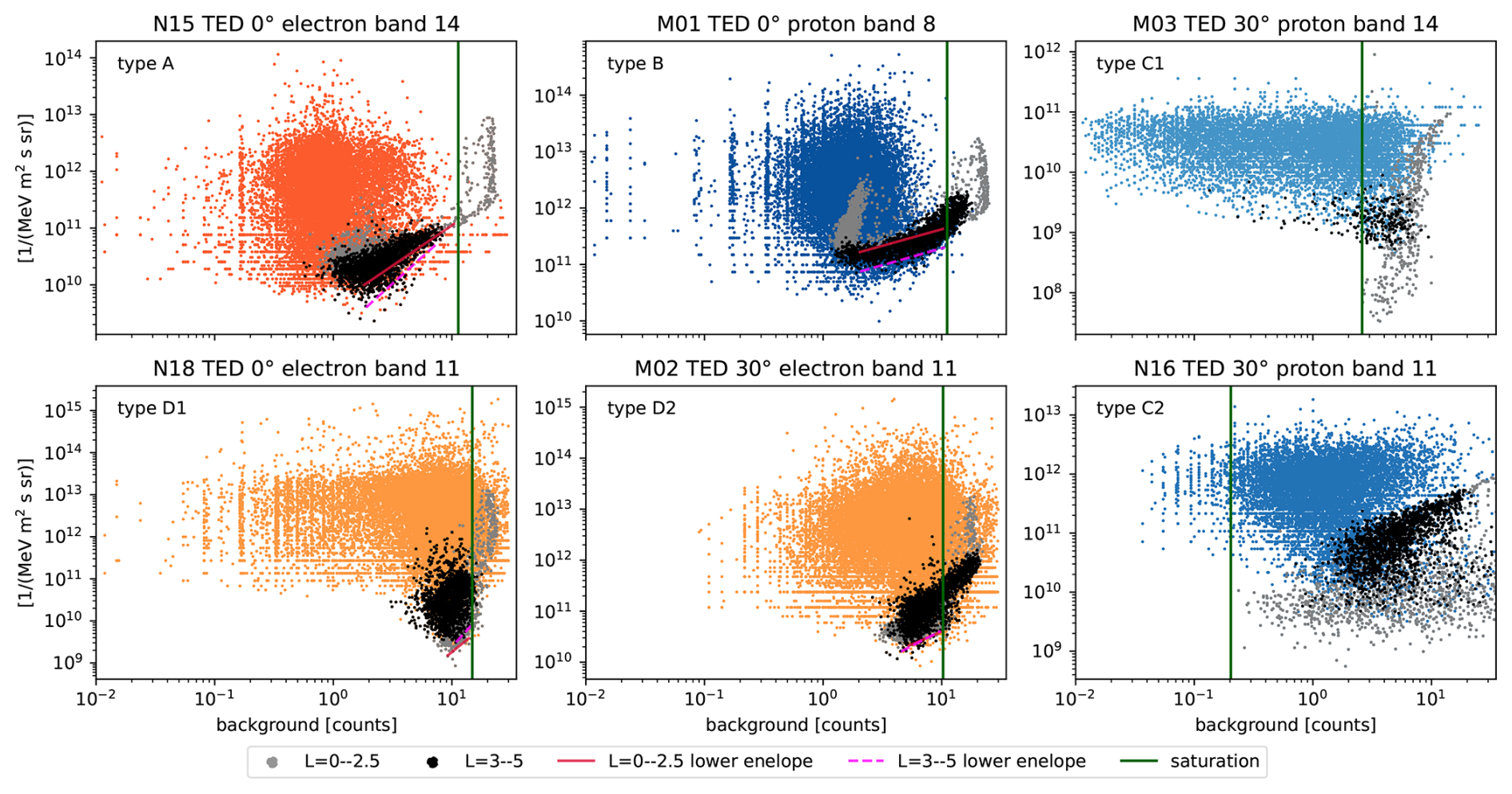
Figure 9 presents the different types of contamination that we found in examining all satellites: “type A” is similar to “type normal” but the contamination seems to depend on particle source. The particle detector is equipped with a magnetic filter that might have a particle specific effect on the contamination. However it is not clear why this applies to some of the channels only. The affected channels are indicated in Tables 2 and 3. The classification has been done by comparing the lower envelopes for all valid background levels. In case that these differ by more than a factor two we labeled it as “type A”. A correction for “type A” should be done as for “type normal” but considering the different kind of contamination (for simplicity this is also done in “type normal”). In case that a channel is also identified as one of the following types, this supersedes the “type A” declaration.

“type B” applies to the proton band 8 on every satellite and both viewing directions. At least partly the distributions are not proportional to background counts. And we observed a different behavior in case of proton or electron contamination. Within the SAA region, enhanced flux is observed at relatively low background values but the neighboring channels 4 and 11 do not observe an enhancement. It is unclear what is going on here. A physical explanation might be that the satellite is negatively changed. But then the charging must always be on the same level because just this channel is affected. If we see charging effects, that would not impact particle precipitation. And charging should more be a issue for high flux regions as the auroral area than for high energy areas. Thus we recomment to not use p 8 on all satellites.

“type C1” seems to be particle specific as well. The subauroral flux seems not or not significantly affected by contamination. Within the SAA however the flux starts orders of magnitude smaller than anywhere else but than saturates almost instantly for increasing background counts. Consequently a correction can only be suggested for expected electron contamination. In case of proton contamination the data should be neglected.

“type C2” is very similar to “type C1” but electron contamination also seems to reduce the observed fluxes. As such any kind of contamination is uncorrectable. This type has only been observed in some channels of N16, which TED detector is officially declared as defect starting from 2006. We recommend to exclude these channels even before 2006.

In “type D” the saturation level is reached also outside typical contamination areas. For D1 no or just minor dependence on background flux below saturation level is observed while D2 shows obvious dependence on background. There is a smooth transition between D1 and D2. A correction might be done as in the “type normal” case but the correction will significantly change data outside of SAA and subsuroral area as saturation level is reached there as well. Supposed that higher fluxes of the energetic particle populations (that are reflected in the background counts) are to some degree occuring simultaneously with increased fluxes of low energetic TED populations at higher L-shells, this correction will act as a high flux filter.

Figure 10 Lower envelope of the contamination for all channels and satellites.

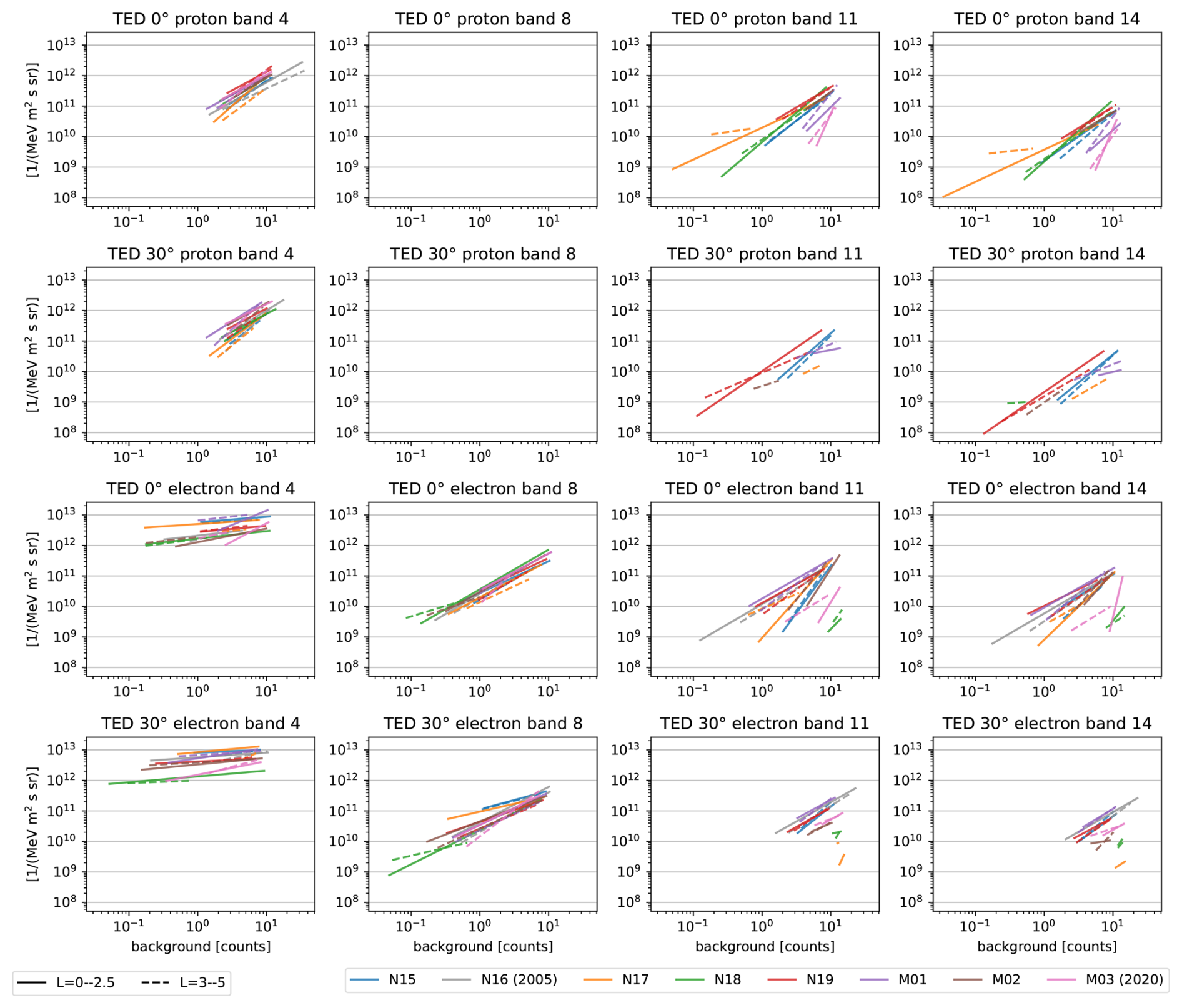
Figure 10 gives an overview on the lower envelopes of all TED channels on all satellites that are not excluded as uncorrectable type. TED 0° electron band 8 shows the best overall agreement of the lower envelopes. Here, the background response seems to be almost identical for contaminating protons and electrons thoughout all satellites. A very weak dependency on background counts is seen in both TED 0°/30° e 4 bands as indicated by the slow rise of the lower envelopes. The reason probably is that high flux values overshadow contamination effects. The strongest inter-satellite differences are typically connected with channels 11 and 14 (and the problematic p 8 bands) where the contamination effect gets stronger in relation to the lower flux values. Note that “type C1” occurs in p 30° 11/14 only while “type D” can be found in the 11/14 bands of p 0° and e 0°/30°. The biggest differences to the other satellites are mostly found for N17, N18, M01 and M03 while no significant outliers have been observed for M02, N15 and N19. However, these differences are channel-specific –and may change over time. The plotted data is given in Tables 2 and 3.

5.2 Application of the Contamination Correction

Figure 11 demonstrates the effect of the suggested contamination correction under different geomagnetic conditions. The correction here has been done with a factor 1, meaning that if below saturation level only the lower contamination envelope has been subtracted. The applied correction method is available as Python code. In case that the background subtraction resulted in negative fluxes the channel has been removed and the particle spectrum fit has been done based on the remaining channels – if available. Period, location and color scale exactly matches to Fig. 6 and thus can be compared the contaminated fluxes and to SSUSI observations.

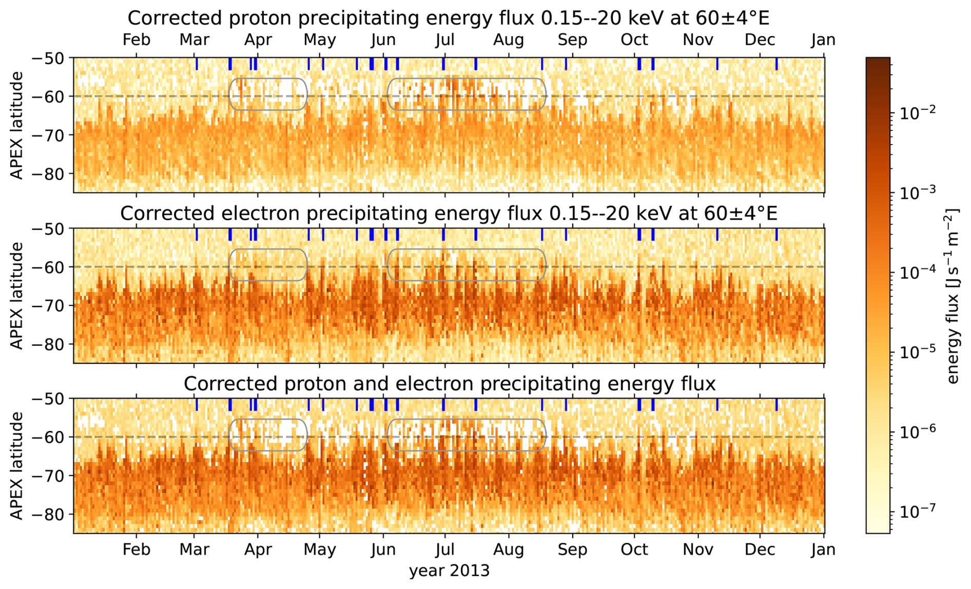
Figure 11 Similar plot as Fig. 6 but with corrected fluxes. Note that the third panel (protons + electrons) contains data only in case that it is available for both particle species.

Starting with the proton precipitating flux, the moderately contaminated periods (outside the marked areas) are now practically cleaned from contamination, as. e.g. seen in early March, May or October. However, the proton correction does not come without the prize of missing data in cases of uncorrectable contamination. Given that this plot shows daily averages on 1° latitude resolution and on a 9° longitude patch the amount of data points per bin is not ideal for a correction attempt designed for average particle fluxes and average background counts. Within the marked heavily contaminated periods about half of the proton data is missing now. It should be said that this is just a minor problem for the atmospheric effects as the electron ionization is typically higher and mostly available after correction. Especially in July there are subauroral proton peaks remaining after the correction. Interestingly SSUSI on DMSP F18 (in contrast to F17) shows peaks in this period as well which are only slightly equatorward of this, so it remains unclear if the corrected fluxes are still contaminated here. Anyhow the overall proton picture is much closer to the SSUSI observations than with using uncorrected fluxes. The electron correction looks very convincing. Even during the heavily contaminated periods no elevated fluxes are seen any more. The proton plus electron precipitating flux shows a much better agreement with the SSUSI observations. Please note that Fig. 11 shows the worst-case scenario, with the strongest background counts occurring at 60° E APEX.

While the contamination is mostly removed now, this method does not replace an inter-comparison of the TED data. However, the corrected TED fluxes should be a better data base to use than the uncorrected fluxes.

Some uncertainty persists in the factor 1. It is not clear how strong natural fluctuations are impacting the results. It might be that at least part of the particle flux above the lower envelope is due to statistical variations that deviate from a direct relationship between background counts and contamination flux – which are not measured simultaneously or on the same location. While the factor 1 should be a good estimation for large ensembles, stronger statistical fluctuations when using just a few measurements might afford a factor > 1 – with the cost of a reduced average (or negative fluxes). Within the scope of this study we can state that the applied correction matches to the SSUSI observations in so far that the subauroral maximum is mostly removed while the auroral pattern persists with flux levels comparable to SSUSI observations. But the limitation of SSUSI's low flux resolution does not allow to quantify or the remaining subauroral contribution.

6 Conclusions

In this study, we investigate the subauroral flux maximum (located at approximately 60° N/S APEX, corresponding to L=4, with a longitudinal focus between 0° and 100° E APEX, most prominent south of the South Atlantic Anomaly) observed in many TED channels. This subauroral maximum is predominantly visible in the vertical proton channels but is also present in nearly all other channels.

Two independent measurements of atmospheric impact contradict the presence of the observed subauroral peak of low-energy particle fluxes under low Kp conditions. Only at higher Kp levels does the expanding auroral oval contribute to low-energy precipitation in subauroral regions. It is important to note that our observational methods are limited to higher altitudes; thus, precipitating energetic electrons with an ionization peak below 80 km would not be detected.

Increased background counts indicate a likely instrumental issue, such as contamination, even though the absolute background levels remain low. The most probable source of elevated TED background counts is energetic electrons from the radiation belt. The increased background in the TED 0° proton and TED 30° electron channels may be attributed to the design of the detector stack.

The vertical channels may be used to derive atmospheric ionization. However, failing to correct for the contaminated subauroral peak – such as in TED 0° proton band 11 (which registers twice the typical auroral proton flux) – would result in subauroral thermospheric ionization rates reaching approximately 14 % of the typical auroral electron ionization rates. This underscores the necessity of a correction method.

Table 1 presents a preliminary latitude-based cutoff approach, limited to channels with a clearly identifiable contamination peak. While this method leads to an underestimation of the precipitating flux (area), contamination appears to be the dominant source of subauroral signals and can be addressed without introducing a longitudinal dependence.

A detailed investigation of all particle channels and their individual contamination behavior (see Sect. 5.1) revealed that all channels are affected by a background count saturation level, above which the data should not be used. Lower envelopes of the contamination, as a function of background counts, have also been identified and may be subtracted as a flux correction.

While many channels exhibit similar crosstalk responses to proton and electron particles, some channels react in a particle-specific manner. The 0 and 30° proton band 8 channels across all satellites show a distinctly different contamination pattern compared to neighboring channels, leading us to recommend excluding these channels from other studies (or at least using them with caution). The same applies to channels in which proton-induced (and partly also electron-induced) background counts appear to suppress the measured particle flux. Additionally, in some channels, the contamination threshold is reached even within the auroral region, meaning that applying a simple threshold-based cut would significantly impact the corrected flux.

The proposed channel- and satellite-specific corrections are summarized in Tables 2 and 3 and can be applied automatically using a provided Python routine (see the additional material for this paper). These corrections are based on TED band flux, background counts, and L-shell, or alternatively allow for manual selection of protons or electrons as the contamination source.

Section 5.2 applies the Python routine to TED data from 2013, demonstrating (in Fig. 11) much better agreement with SSUSI observations. Limitations of the correction include: (a) negative (i.e., missing) data due to over-correction, which primarily affects short-term binned proton data; and (b) residual high subauroral proton fluxes, which may be either accurate (e.g., when compared to SSUSI F18) or inaccurate (e.g., when compared to SSUSI F17).

We should note that our proposed correction method is not limited to the recent netCDF-files. It should also work with the older bin-files or a corrected netCDF algorithm without high-background cutting – even though a user should think about setting a maximum background flux (like the saturation threshold) that still allows for a reasonable subtractive correction, a certain proportion maybe. In case of the “type D” contamination a different background handling in the netCDF-files would be clearly beneficial.

Further studies may be valuable to assess the impact of fluctuations and determine whether a more aggressive correction is warranted. Additionally, note that the correction functions are based solely on data from 2013 (and for N16, on 2005; for M03, on 2020); detector degradation or different voltage settings may alter the contamination effect in other years. Therefore, follow-up studies are encouraged.

Appendix A: Additional Material: Python Code

The Python routine TEDcorrection.py contains the information from Tables 2 and 3 as well as the contamination type. It provides the suggested correction functions based on TED particle flux, background counts and L-shell as used in Fig. 11. An example data set and the application of the correction is provided as well.