First results from the Juice magnetometer during the Lunar-Earth Gravity Assist

Before reaching the Jovian system in 2031, the ESA Jupiter Icy Moons Explorer (Juice) spacecraft will perform three Earth flybys. As well as providing gravitational assistance, these flybys are prime opportunities to assess performance and undertake in-flight calibration of the science payload in a well-understood environment. The first such interval occurred in August 2024, dubbed the Lunar-Earth gravity assist (LEGA) as it included a pass by the Moon in advance of the approach to Earth. The unique spacecraft trajectory allowed for sampling of various regions of the magnetosphere before exiting into the solar wind. In this paper, we report on the performance of the Juice magnetometer instrument (J-MAG) during the LEGA. These are the first reported results from J-MAG in flight. J-MAG comprises three sensors – two fluxgate vector sensors and one Coupled Dark State Magnetometer (CDSM) scalar sensor – all of which were operational during the LEGA period. This represents the first time in the mission that the scalar sensor has operated in its nominal state. Here, we analyse J-MAG observations during key periods of the flyby. As well as inter-sensor comparison, we assess J-MAG data against geomagnetic field models during the approach to Earth, and compare with measurements from other spacecraft at the Moon and in the solar wind, which allow us to make suggestions for future calibration activities. Overall, the three sensors showed excellent performance at this early stage in the mission and confirmed that the scalar sensor meets the requirements for in-flight calibration of the fluxgate sensors at Ganymede. The LEGA also demonstrates the potential value of using cruise phase measurements for scientific exploration and solar wind monitoring.

1 Introduction

The European Space Agency's Jupiter Icy Moons Explorer (Juice; see Grasset et al., 2013) launched in April 2023. As part of the mission cruise phase, the spacecraft performs three gravity assists at Earth, the first of which occurred in August 2024, and included a flyby of the Moon. The Lunar-Earth Gravity Assist (LEGA) was an excellent opportunity to gain an early indication of spacecraft and instrument performance in a known environment, allowing for preliminary calibration activities and some exploratory science. In particular, the conditions and phenomena seen in some regions of Earth's magnetosphere, and the performance of J-MAG within them, are indicative of those expected at Ganymede.

In this paper we report on the operation and results from the Juice magnetometer instrument, J-MAG, during the LEGA. There are three sensors that comprise the J-MAG system: the outboard sensor (henceforth referred to as OBS), the inboard sensor (IBS), and the scalar sensor (SCA). All three are mounted on a 10.6 m boom, away from the body of the spacecraft. OBS and IBS are fluxgate magnetometers that draw heritage from those flown on missions such as Cassini (Dougherty et al., 2004), Solar Orbiter (Horbury et al., 2020), Rosetta (Auster et al., 2007), and Bepi Colombo (Heyner et al., 2021). SCA is a Coupled Dark State Magnetometer (CDSM), an optically-pumped scalar magnetometer based on two-photon spectroscopy of free alkali atoms. It measures the Zeeman shift experienced by gaseous ⁸⁷Rb atoms in the presence of a magnetic field, where the energy level splitting is proportional to the field strength. To determine the field magnitude at varying angles to the optical axis, two resonance modes (longitudinal and transverse) are used. For further background on the scalar sensor engineering and operation see, e.g. Pollinger et al. (2018) and Amtmann et al. (2024). Juice is the first mission to use such a magnetometer outside of Earth orbit.

This paper focuses on demonstrating the overall performance of the J-MAG system during the LEGA, without detailed discussion of calibration procedures. This is the subject of future study and can only be completed with additional data beyond this early stage of the mission. We do, however, outline the steps taken so far and those that remain to be refined. The report is structured as follows: first we describe the LEGA trajectory and solar wind context in which it occurred. We then describe the timeline of J-MAG operation, with a particular focus on the unique challenges faced by SCA. We outline the calibration process for the LEGA, and then we report the J-MAG measurements, making comparisons to those from other spacecraft and models where appropriate. This is broken down by particular regions of interest including the close approach to Earth, the lunar pass, the exit from the magnetosphere, and the journey into the solar wind. We conclude with a summary and outlook for future J-MAG operation and calibration opportunities.

2 LEGA trajectory, timeline, and environment

The spacecraft trajectory relative to Earth is shown by the black dashed line in Fig. 1. This depicts the X–Y plane in the Geocentric Solar Ecliptic (GSE) coordinate system, with markers showing the spacecraft position at midnight of each day. The portions of the trajectory for which J-MAG was recording science data are highlighted in red. An approximate magnetopause is shown by the solid black line, derived from the Shue et al. (1998) empirical model parametrised using average solar wind conditions over the flyby (see Fig. 2).

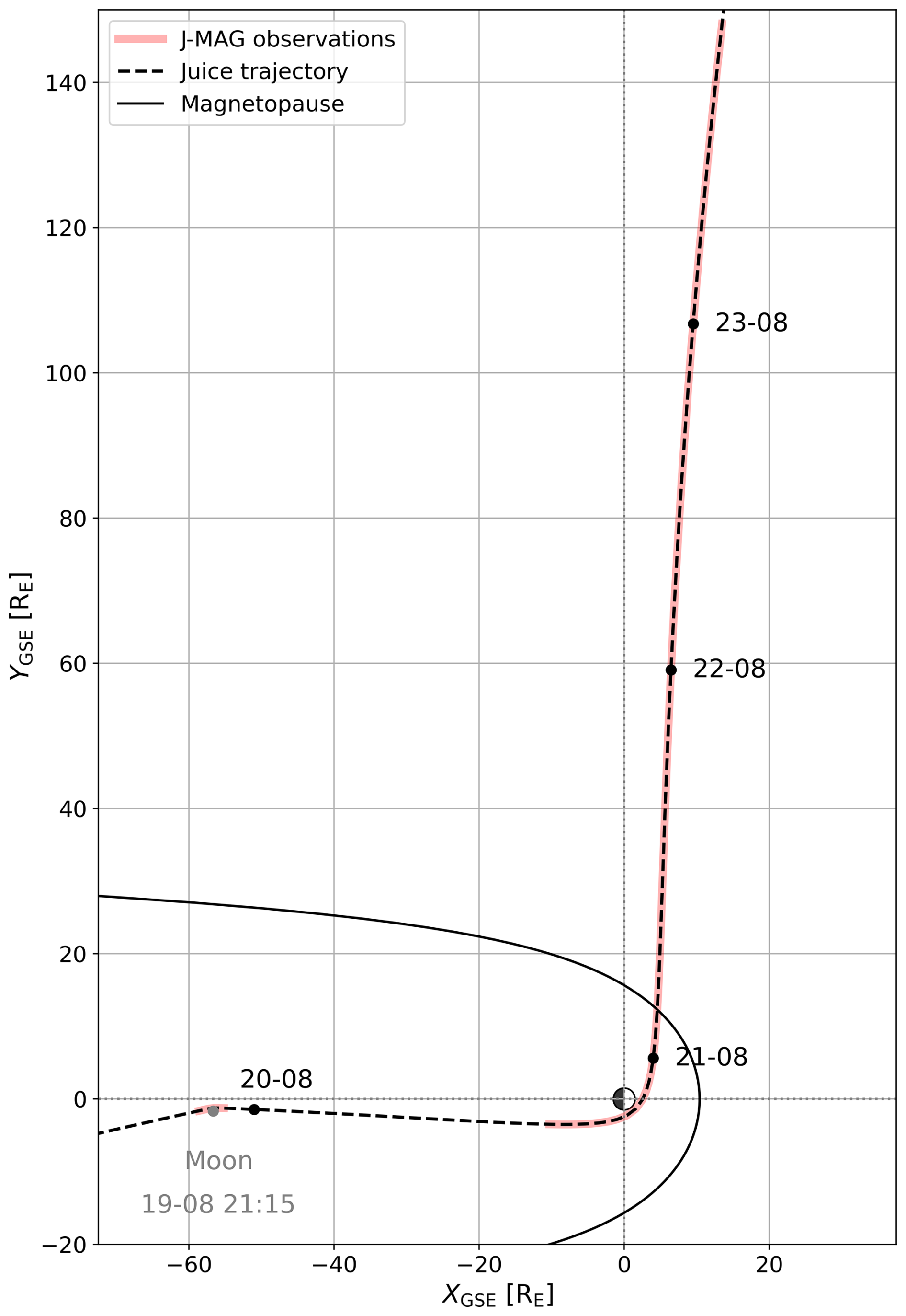
Figure 1 Orbital trajectory of Juice spacecraft during the LEGA, shown in the GSE X–Y plane, in units of Earth radii. Dashed black line shows spacecraft path, with the position at midnight of each day marked with a black dot. The portions of the flyby for which J-MAG was recording science data are highlighted in red. Solid black line shows an approximate position of the magnetopause as predicted by the Shue et al. (1998) empirical model, parametrised with average solar wind conditions during the LEGA period. The position of the Moon at lunar closest approach is also marked.

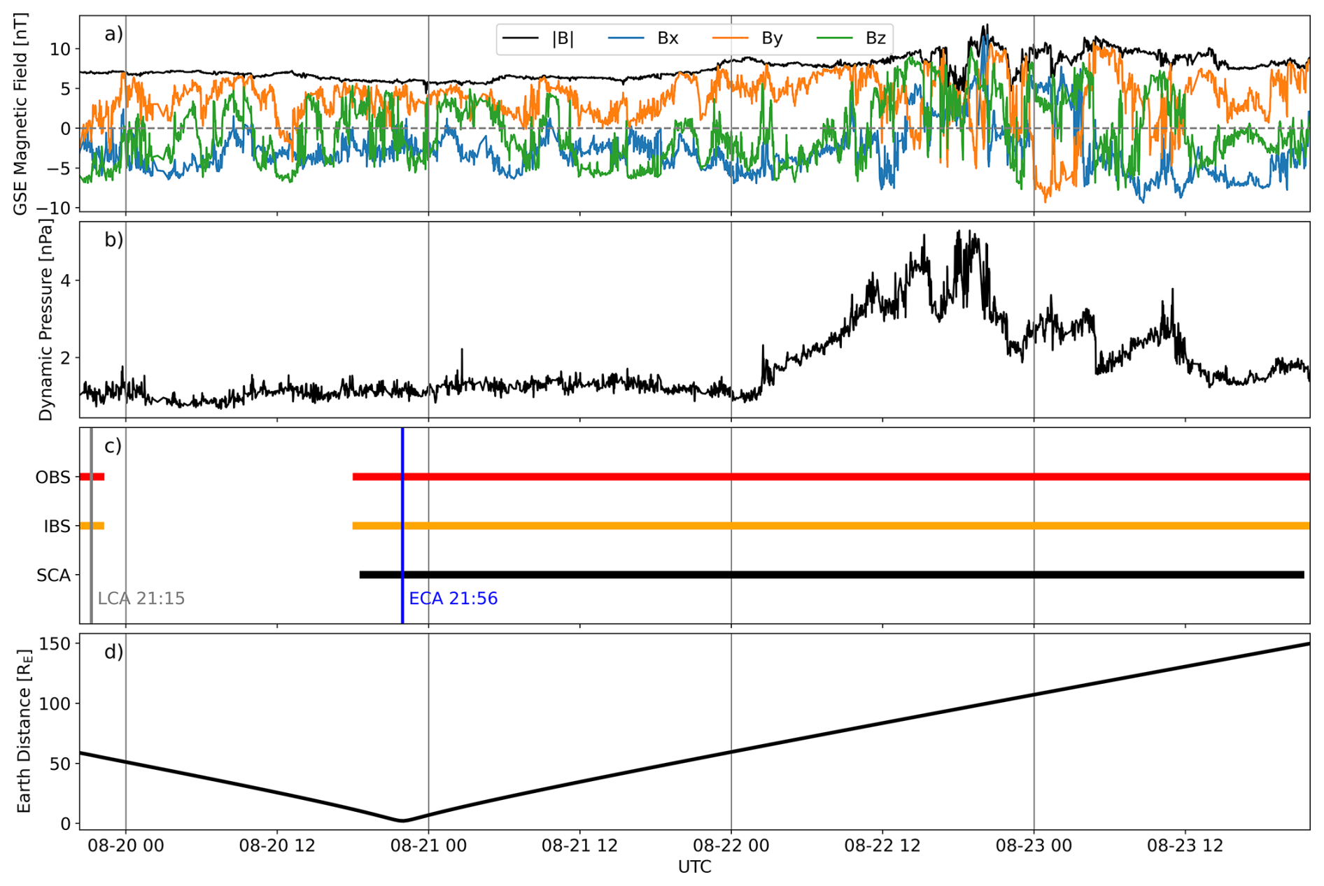
Figure 2 Flyby context and timeline. Panel (a) shows the interplanetary magnetic field (GSE) from the OMNI database, that is, measured at L1 and algorithmically propagated to Earth's bow shock. Panel (b) shows the solar wind dynamic pressure during the flyby period. Panel (c) shows a timeline of J-MAG sensor operation, with the lunar closest approach (LCA) and Earth closest approach (ECA) marked. Panel (d) shows the distance of Juice from Earth.

Juice approached from the nightside, first encountering the Moon on 19 August 2024. For a period of around 40 min, the spacecraft was eclipsed by the Moon, therefore running on battery power and limiting operations. Shortly after eclipse, Juice made its closest approach to the Moon at 21:15 UTC, at which the minimum distance from the spacecraft to the centre of the Moon was ∼2500 km, or approximately 1.5 lunar radii. At this point, the spacecraft was deep in the magnetotail, close to the Sun-Earth line. J-MAG made observations for a two-hour period across the lunar pass. In Sect. 4.2, we look at this phase of the flyby in more detail.

Following the lunar encounter, Juice continued its approach towards Earth, largely following the Sun-Earth line but veering to the dawn side. The trajectory took the spacecraft round the dayside, headed duskward. Closest approach was made on 20 August at 21:56, at which the distance to the centre of Earth was around 2R_E, or ∼13 000 km, taking the spacecraft deep into the inner magnetosphere. J-MAG started recording science data around 4 h before closest approach.

Juice exited the magnetosphere at around 03:00 on 21 August, crossing the magnetopause, transiting the magnetosheath, and passing through the bow shock around 5 R_E sunward of the terminator (see Sect. 4.3 for more detail). Thereafter, Juice continued duskward and marginally sunward into the pristine solar wind, with J-MAG operating continuously before switching off on 23 August.

Figure 2 shows the solar wind context and a more detailed timeline of J-MAG operation during the LEGA. Panel a shows the interplanetary magnetic field (IMF) as retrieved from the OMNI database (King and Papitashvili, 2005). The high-resolution (1 min cadence) dataset comprises solar wind measurements made by spacecraft at the L1 Lagrange point (e.g. ACE, Wind, or DSCOVR) and algorithmically propagated to Earth's bow shock, making it the standard and most complete dataset for the solar wind conditions driving Earth's magnetosphere. In this time period OMNI data originate from the Wind spacecraft, the IMF measurements provided by the Magnetic Field Instrument (MFI; Lepping et al., 1995), and plasma observations from the Solar Wind Experiment (SWE; Ogilvie et al., 1995). The second panel shows the solar wind dynamic pressure, also provided by OMNI. This quantity compounds solar wind mass density with its speed, that is, P_d=ρV². Dynamic pressure is a key metric for assessing the energy input to the magnetosphere, with higher dynamic pressures typically compressing the magnetosphere and stimulating geomagnetic activity. The position of the subsolar bow shock nose (as estimated empirically and for which the OMNI data correspond) varied somewhat throughout the LEGA period. For 19–21 August, this position averaged around 14.25 R_E (X_GSE). Early on 22 August the bow shock position began to move Earthward, reaching a minimum of 11.4 R_E at 15:36 and averaging 12.75 R_E across the day. It gradually recovered over the following day, averaging 13.3 R_E for 23 August. This mirrors the solar wind dynamic pressure profile shown in Fig. 2b. Panel c shows a timeline of operation of the three J-MAG sensors, OBS, IBS, and SCA. Also marked on this panel with vertical lines are the moments of closest approach to the Moon and to Earth. Panel d shows the distance of the spacecraft from Earth throughout the flyby.

Breaking the J-MAG timeline down by sensor, OBS and IBS sensors were switched on at 20:19, just shy of an hour ahead of the lunar closest approach (21:15). Both fluxgates remained on until 22:14 and made observations at 16 Hz cadence. SCA was not operational during the lunar phase (see Sect. 2.1). Ahead of the Earth flyby on 20 August, OBS and IBS took measurements from 18:01, with SCA starting shortly after at 18:34. All three sensors then remained on for several days, switching off when the spacecraft was well into the solar wind on 23 August, SCA at 21:22, OBS and IBS at 21:53. At this point, Juice was 150 R_E from Earth.

We see that, during the early portion of the flyby, the solar wind exhibited relatively quiet and stable conditions with low dynamic pressure (solar wind speed was slow, at around 300 km s⁻¹), low magnetic field magnitude and few large variations. There were, however, periods of negative B_Z which may have driven reconnection at the magnetopause and short periods of activity. Later on, after Juice left the magnetosphere, activity in the solar wind increased, with a ramp up in both magnetic field magnitude and dynamic pressure. There is also a notable period of rotation in the magnetic field at the point of highest dynamic pressure. This provided an excellent opportunity to compare the structure observed by J-MAG with that seen by spacecraft at L1 (see Sect. 4.3).

2.1 Scalar sensor operation

The operation of the scalar sensor is considerably more complicated than the two fluxgate sensors. In this section we detail the process used during the LEGA. The three Juice Earth gravity assists (EGAs) present crucial opportunities for SCA as they are the only times during the cruise phase when SCA can make a direct measurement of the external field magnitude. By this we mean that the CDSM is not suitable for measurements below 100 nT with high accuracy (Ellmeier et al., 2024) and so in the solar wind an auxiliary DC field of order 2000 nT is applied via the auxiliary coil solenoid fitted around the sensor optical axis. This lifts the field magnitude in the volume around the sensor way above the 100 nT limit, thus enabling detection of the external field component along the SCA optical axis with high accuracy. To compare fluxgate and SCA data in the solar wind, one must first project the measured vector from the fluxgates onto the SCA optical axis as it is only sensitive to the component of the field strength along this direction.

The duration of the lunar pass was too short for SCA to heat up and stabilise, and with relatively low fields in the magnetotail, the auxiliary coil would be required. For these reasons it was agreed not to operate the SCA during the lunar pass. For the close approach to Earth, the challenge was to switch on while still in a low field environment with the auxiliary coil enabled and then switch off the auxiliary coil once the external field increased to a point where it was comfortably above the detection limit. The approach taken for this was as follows.

SCA was switched on while still in a relatively low field environment, the cell and laser diode were heated to their operational temperatures, and the auxiliary coil was switched on to apply a constant DC field. Resonance sweeps were performed while operating in n₂ (longitudinal) resonance mode (Pollinger et al., 2012). This is the standard approach to get SCA into nominal field measurement mode. Then, as the external field increased, the auxiliary coil field was correspondingly ramped down such that the field in the vicinity of the SCA sensor remained above 100 nT at all times in order to avoid losing lock. The timing of the auxiliary coil ramp down profile was estimated in advance by field modelling. As the angle between the external field and the optical axis strayed out of the n₂ operation cone, the SCA was switched to n₃ (transverse mode) at the start of the auxiliary coil ramp down. This was performed successfully, marking the first time in the mission that the n₃ mode was used. When the auxiliary coil current decreased to zero, SCA was free running in n₃ mode and measuring the true external field magnitude. This is the first time the SCA was operated nominally, meaning that the angle of the magnetic field was taken from a fluxgate sensor, and based on this the resonance was chosen. This covered approximately four hours centred on the closest approach. There were two mode switches during the LEGA, from n₂ to n₃ and then back again. They happen at around 60° magnetic field angle, 0–60° n₂, and 60–90° n₃.

At external fields below 100 nT, a firm Zeeman resonance lock is not possible under all operating conditions. Here, generating valid science data within the SCA specifications is also not possible (Ellmeier et al., 2024). As a consequence, SCA was switched back on with a constant auxiliary coil field some time later. SCA remained in that state from that point until the end of the J-MAG operational period. The timeline of SCA operation was executed as expected from the modelling predictions.

3 Calibration summary

Here we describe the calibration steps taken thus far, clarify which processes have been applied to the data presented, and outline calibration activities that have not yet been applied and will take place later in the mission. Please note that a fuller description of the J-MAG calibration process is planned for a future work, and so we present only a brief summary. The process described largely applies to the fluxgate sensors. For the LEGA, only data from the inboard sensor underwent each step of the calibration process described here. This is due to the temperature variations seen at OBS during the LEGA period due to the OBS heater, which was required to be on during the inner cruise in order to generate sufficient load on the J-MAG DC-DC converter to enable safe SCA operation during the fly-by. Due to the short operating period, there was not enough time for OBS to reach thermal equilibrium before the flyby. IBS was operated without a heater and so the sensor temperatures were more stable. Therefore, the IBS data were determined to be more reliable. It is known that fluxgate magnetometer offsets and gains are affected by changes in temperature (Magnes et al., 1998). This is not an issue unique to J-MAG (see, e.g. Alconcel et al., 2026, for a recent discussion on temperature effects on the Cluster magnetometers), but the limited operations on JUICE during early cruise mean that the specific response of J-MAG to temperature variation is yet to be fully characterised in flight. The consolidated J-MAG data product used in this LEGA study is therefore constructed from IBS data. These are the data presented in the rest of this paper unless otherwise specified.

The vector magnetic field data have undergone the following calibration process, which can be summarised in three main steps:

1. Ground calibration. Application of calibration parameters determined from pre-flight instrument testing. This includes range-dependent scaling factors to convert measurements from engineering units to nT. Ground-determined offsets are subtracted, and a matrix is applied to correct for non-orthogonality and gain. This is the base level calibration that is fixed and applied automatically to all observations.

2. In-flight corrections. Subtract preliminary in-flight offset perturbations calculated using the Hedgecock (1975) method in the solar wind after the flyby. Rotate from sensor frame to geophysical coordinate system. This includes first rotating between inboard and outboard sensor coordinate systems using a preliminary matrix calculated in-flight from comparison of solar wind intervals. A small rotation correction to the definition of this frame, calculated from comparison with geomagnetic field models (see Sect. 4.1) is then applied. From here, the data can be recast in geophysical coordinates (e.g. GSE) using transformations retrieved from Juice SPICE kernels.

3. Additional processing. Remove problematic or unwanted intervals, e.g. signals from scalar sensor sweeps. The data may then be resampled to any desired cadence.

The J-MAG data shown in Figs. 4, 7, and 8 have had the above process applied. We consider the current J-MAG in-flight calibration to be preliminary as there are some calibration processes still to be developed, and several calibration parameters to be refined once more data are available, such as the frame transformation matrix used in step 2 above.

At this stage in the Juice mission, only a relatively limited quantity of J-MAG observations have been made, as the scientific payload is not yet operating continuously. Most of the operational periods thus far have been for the purposes of payload functional checkouts. These times are typically dominated by instrument and spacecraft tests, which can introduce interruptions and disturbances to J-MAG observations. For some calibration parameters, such as offset-perturbations, we require extended periods of “clean” data for the most reliable estimates. This is planned for later in the mission's cruise phase. Continuous operation will allow for tracking of offset drifts and characterisation of their response to external factors, e.g. changes in temperature, instrument power consumption, or spacecraft activities. This may include the use of thermal modelling of the boom.

A better understanding of temperature effects on each of the sensors will allow for an assessment on discrepancies between fluxgate data and inform the process for combining measurements from all three sensors into one consolidated J-MAG product, which was not possible for the LEGA.

Alignment calibration, arising from comparison of J-MAG data with geomagnetic field models during the flyby, is also only preliminary at this stage. This will be refined in the two subsequent Earth flybys, and via operation of the Juice Magnetometer Alignment Calibration System (JACS; Matsuoka et al., 2019). This comprises two orthogonal coils that, when supplied with a current, create an external field that can be used to assess changes in fluxgate sensor alignment. See Sect. 4.1 for further discussion on alignment calibration.

Additional calibration activities that may take place include filtering to remove any noise sources from within the instrument or arising from spacecraft activities, and investigating potential timing issues. Future functional checkouts include plans for dedicated timing tests with each of the sensors operating in burst mode to confirm that measurements are timestamped correctly and consistently.

4 J-MAG measurements

In this section we examine J-MAG observations during the LEGA, broken down by region of interest. To assess performance, we compare with other spacecraft measurements and empirical models where possible.

4.1 Earth flyby

We start by examining the performance of each of the sensors within Earth's magnetic field. Figure 3a shows the magnetic field magnitude measured by each of the three sensors in the two hours around closest approach. Artificial offsets of +100 and +200 nT have been added to IBS and OBS, respectively, in order to make all three traces visible. At this scale, the three measurements lie exactly on top of each other when plotted without offsets applied. Panel b shows a zoom on the few minutes around peak field, but with no artificial offsets. OBS and IBS data are shown at a cadence of 16 Hz, while SCA is 1 Hz. We can see that all signals are very clean, follow the expected pattern at close approach, and at the peak in field magnitude, the fluxgate sensors agree within 3 nT (out of ∼4100 nT) of the scalar sensor.

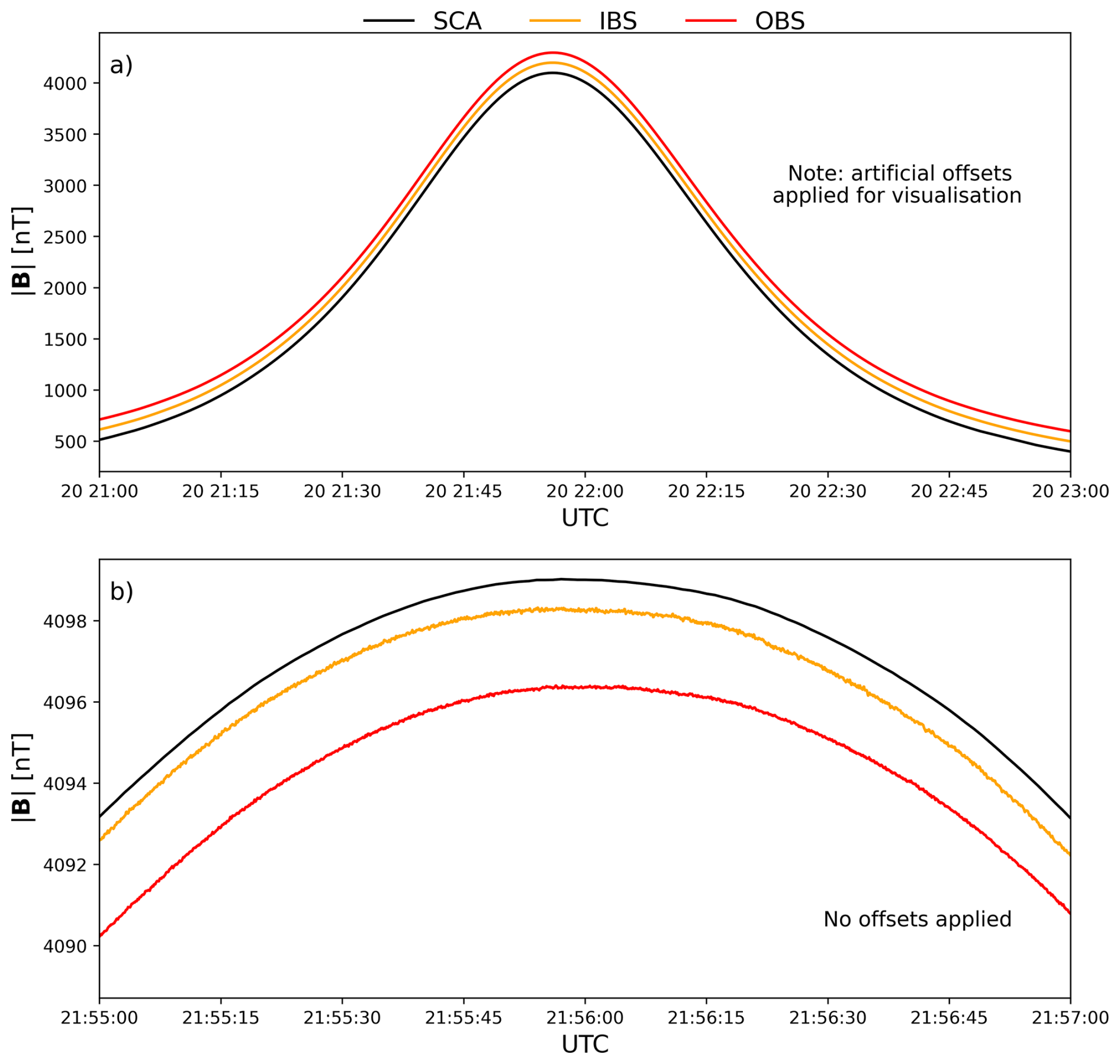
Figure 3 Magnetic field magnitude of the three J-MAG sensors around the Earth closest approach. Panel (a) shows two hours centred on closest approach, with artificial offsets of +100 and +200 nT added to IBS and OBS data, respectively, to aid visualisation at this scale. Panel (b) is a zoom on the peak field at the two minutes of closest approach (with no artificial offsets applied) showing slight differences between sensors. Note the data presented here have undergone only ground-based calibration (i.e. step 1 in Sect. 3).

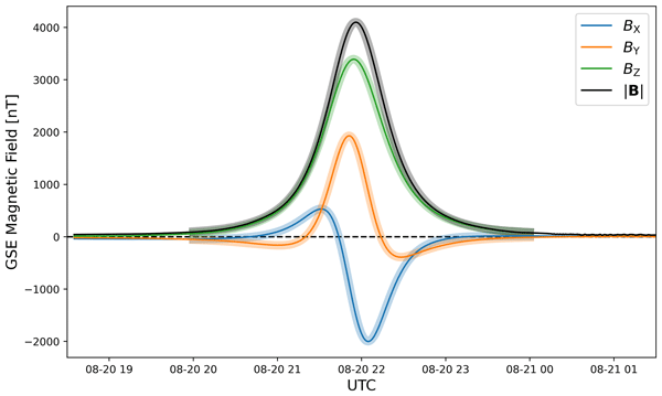
Figure 4 shows the magnetic field vector measured by J-MAG during the Earth flyby in GSE coordinates (thin, solid lines). Overlaid (thick, transparent lines) are the results of modelling the geomagnetic field expected to be seen over the flyby trajectory. The internal component of the field model comes from the latest version of the International Geomagnetic Reference Field model (IGRF-14; see Alken et al., 2021; Madsen et al., 2026). Externally-driven perturbations arising from solar wind interaction with the magnetosphere are then added using the Tsyganenko 2001 empirical model (see Tsyganenko, 2002a, b, for details), parametrised using solar wind conditions from OMNI during the flyby (i.e. those in Fig. 2).

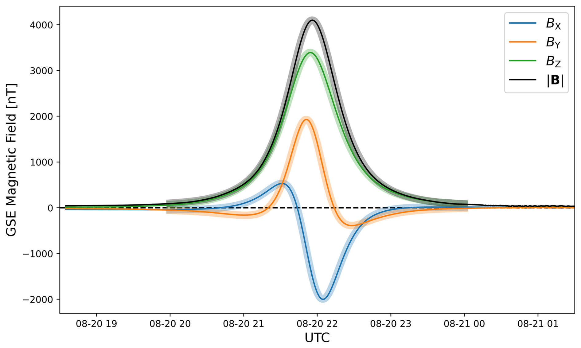
Figure 4 Magnetic field vector measured by J-MAG around Earth closest approach (solid lines), overlaid with model field from IGRF-14 and Tsyganenko 2001 model for the Juice LEGA trajectory (thick, transparent lines), all in GSE coordinate system.

As discussed in Sect. 3, by comparing J-MAG observations with the modelled field, we can make an initial calibration estimate. Specifically, we look to see if there is any potential misalignment of the sensors with respect to the defined science coordinate systems. Initially, we see a maximum difference between the observations and model of around 40 nT. By performing a minimisation, we determined that a small rotation of less than 1° in each axis can reduce the maximum difference between the measured and modelled field at any point to ∼20 nT, which we consider very good agreement in this high field environment. It is believed that much of the remaining discrepancy may be physical, instances where the models do not accurately capture the changing conditions, particularly on the edges of the flyby period. This small rotation has been applied to the data displayed in Fig. 4, as well as subsequent Figs. 7 and 8 which explore observations of the outer magnetosphere and solar wind. This aspect of calibration is still preliminary and will be refined in future Earth flybys (see Sect. 3).

The alignment correction applied here is needed to address several potential sources of error. The Juice magnetometer boom is very long (10.6 m) and comprises three hinged segments. While excellent for electromagnetic cleanliness, this comes with increased risk of mechanical instability that may cause sensors to change their displacement or rotate relative to each other and the spacecraft, meaning measurements are not truly made in their nominal defined frames. There also may be uncertainties in the comparison with field models. Though the empirical models are parametrised with solar wind conditions during the flyby, they will not capture all transient field deviations caused by magnetospheric dynamics and processes such as field aligned currents. The modelling comparison also relies on accurate spacecraft ephemeris to reconstruct Juice's path through the Earth field. It is understood that the position uncertainty during flybys is generally of order 10 km, reducing to 10 s of metres at closest approach. A sensitivity analysis for this and future Earth gravity assists is planned for future work.

All of this can result in the J-MAG sensor frames appearing to be being misaligned with their definitions, meaning the rotation calculation here may represent more of an effective alignment correction than true rotation. By monitoring this discrepancy over subsequent Earth flybys and usage of the JACS coil, we will be able to establish whether this misalignment remains constant (and can therefore be corrected by rotation), or whether it changes and represents an uncertainty arising from other factors. In this particular flyby, it is possible that the limited operation window and steep temperature gradients are likely to have a greater effect on measurement to model deviations than misalignment.

4.2 Lunar flyby

Figure 5 shows the position (in GSE coordinates) of Juice relative to the Moon during the lunar phase of the LEGA. Also shown are the positions of the two spacecraft of the Acceleration, Reconnection, Turbulence and Electrodynamics of the Moon's Interaction with the Sun mission (ARTEMIS; Angelopoulos, 2011). These two probes were formerly part of the Time History of Events and Macroscale Interactions during Substorms mission (THEMIS; Angelopoulos, 2008), launched in 2007 in Earth orbit to study the dynamics of Earth's magnetosphere. In 2010, two of the five THEMIS probes were re-directed to enter a lunar orbit, where they continue to explore the magnetotail when the Moon is on the night side, and function as near-Earth solar wind monitors when the Moon is on the dayside. In Fig. 5, Juice's position is shown in red, with ARTEMIS P1 and P2 in blue and purple, respectively, while the Moon is shown in grey. The lines show the trajectories over the period for which J-MAG was measuring, with the final positions of the bodies in this time period shown with markers.

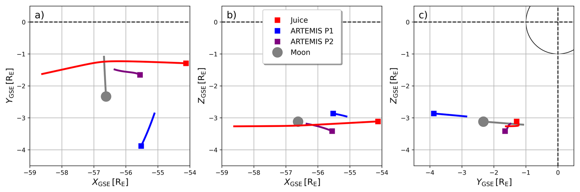
Figure 5 Orbital trajectories of Juice, the two ARTEMIS probes, and the Moon during the lunar pass, 19 August 20:20–22:30. All positions in Earth radii, GSE coordinate system, shown in all three planes. Final positions of the bodies in this period indicated with markers.

Juice passed close to both the ARTEMIS probes, though significantly closer to P2. At the time of lunar closest approach (21:15), Juice was approximately 6600 km (∼1 R_E) from ARTEMIS P2, and 16 600 km (∼2.6 R_E) from P1, while the two ARTEMIS probes were separated by 12 000 km (∼1.9 R_E). At these distances, one can expect good agreement in the large-scale structures seen by all spacecraft, and we therefore find it interesting to compare J-MAG observations with those from the fluxgate magnetometers aboard ARTEMIS (Auster et al., 2008). This is shown in Fig. 6 where the magnetic field measurements from all three spacecraft are plotted in GSE. Data for all three spacecraft are shown at 16 Hz. Here we show OBS and IBS data separately, with OBS in red and IBS in yellow. Offsets of the J-MAG sensors have been adjusted to best match ARTEMIS data for this comparison. The shaded area marks the time for which Juice was in eclipse, and a vertical line marks the point of closest approach to the Moon.

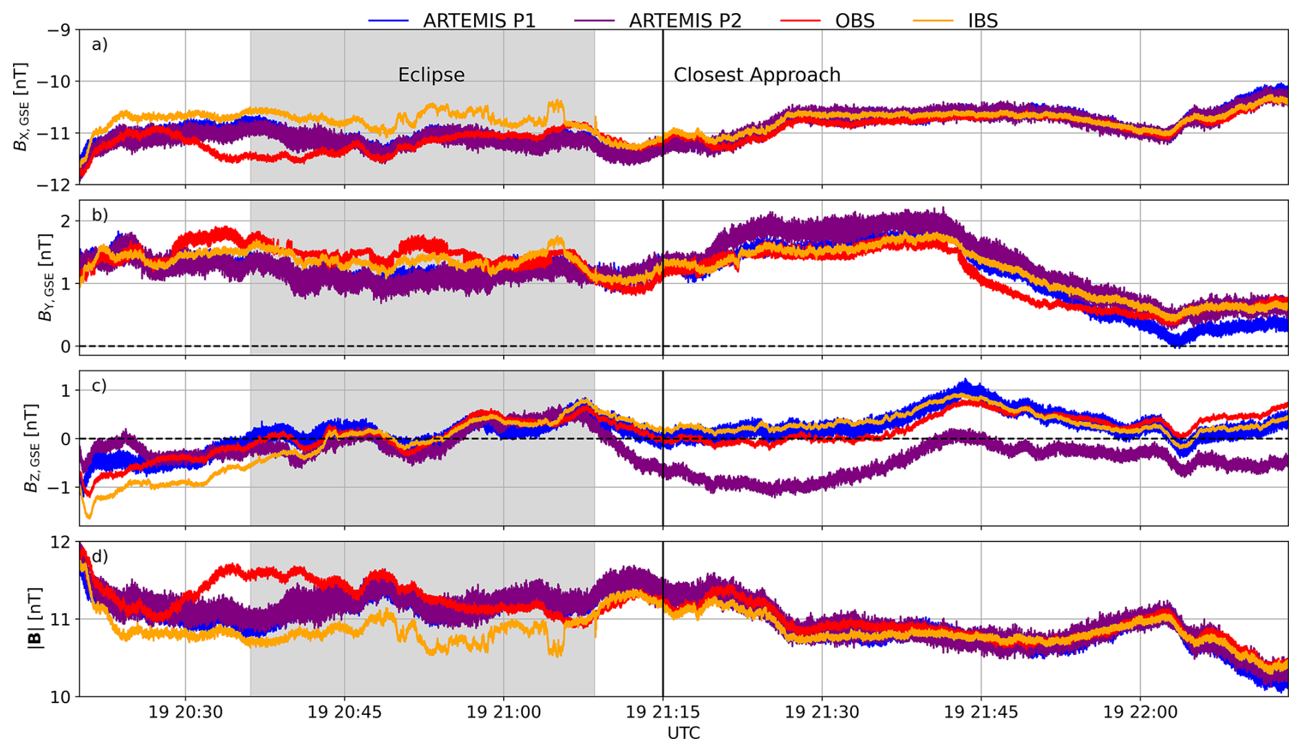
Figure 6 Magnetic field measurements from J-MAG OBS and IBS during the lunar pass, overlaid with observations from the two ARTEMIS probes, all in the GSE coordinate system. Panel (d) shows the field magnitudes. Shaded area indicates the period in which the spacecraft was in an eclipse, and the solid vertical line marks the time of lunar closest approach.

We can make several observations from this short window of data. It is immediately noticeable that both J-MAG sensors show very clean signals, with the level of noise significantly lower than in the corresponding ARTEMIS measurements. This is yet another excellent demonstration of the instrument quality and magnetic cleanliness of the spacecraft (Engelke et al., 2023). Over the two-hour period, the field is dominated by a strong X-component, which makes sense given the position in the magnetotail. Overall, the observed fields are relatively stable, with the maximum field variation around 2 nT. This makes for an excellent opportunity to probe any differences in the four signatures.

There are some discrepancies between the two ARTEMIS probes. This is most notable in the GSE z axis, where they report a difference of up to about 1 nT in the latter portion of the flyby. While curious, this is not totally unexpected given their spatial separation. More puzzling, however, are the differences seen between the two J-MAG sensors. The second half of the flyby, after closest approach, shows generally good agreement, however, significant differences are seen in the earlier portion of the flyby. We see that OBS measures a larger field magnitude, primarily in the GSE x axis, and is at points nearly 1 nT larger than IBS and around 0.6 nT larger than the two ARTEMIS probes. In this period IBS generally sits at a lower magnitude than ARTEMIS, and shows an amount of fluctuation.

We offer some possible explanations for these discrepancies. The lunar pass occurred almost immediately after the instrument was switched on. This means that there was a steep temperature gradient at the time as the sensors and electronics began to warm up. The period of eclipse is also likely to have had an effect on the instrument temperatures, both in terms of the shadow, and the restricted operation of other spacecraft processes while running from battery power. As discussed earlier, temperature is known to affect magnetometer offsets, which may explain the differing behaviour of IBS and OBS. It appears that these irregularities mostly settled after around an hour of operation. In future we would recommend that J-MAG be switched on several hours in advance of any period considered crucial for recording science or calibration data in order to allow for temperature equilibrium to be reached.

As well as relative drifts between the two J-MAG sensors, which we may attribute to temperature fluctuations, there were also some sharp disturbances of order ∼0.5 nT seen by IBS during the eclipse period, most notably at around 21:05, and primarily in the GSE x and y axes. When the data are viewed in the J-MAG OBS frame, the disturbance is seen in the x and z axes, which are perpendicular to the magnetometer boom by definition, with no detectable signature in the y axis. It is therefore believed that a current source along the boom harness may be responsible for the signal seen by IBS, where a field generated by current aligned with the J-MAG y axis would manifest in the other two axes. To create a field perturbation of order 0.5 nT, say, 10 cm away from the source, a current of 0.25 mA would be required, which may be plausible given the boom electronics.

This may also explain why it was not seen by OBS, which is mounted 3 m further along the boom, very close to the tip. Two other instruments are placed between the two fluxgates, the radio wave instrument antennae and search coil magnetometer – both of the Radio and Plasma Wave Investigation (RPWI) suite (Wahlund et al., 2024). Therefore, as well as the cabling from the OBS and SCA sensors, IBS also has harnesses from these other instruments running past it, making it more susceptible to electrical disturbance.

We note, however, that the fact we are able to distinguish disturbances at this scale is a testament to the magnetic cleanliness of the spacecraft and the low noise level of J-MAG. While curious, the magnitude of these fluctuations is small and does not provide much concern with regard to J-MAG EMC requirements (e.g. DC offset at OBS<2 nT), provided we can ensure more stable temperatures during continuous operation at Ganymede (Brown et al., 2019).

It is likely that a combination of factors contribute to the OBS and IBS discrepancies here, and further investigation into sensor behaviour shortly after switch-on and during temperature changes will help to confirm the source of what we see here. Despite the initial calibration, unstable temperatures, and possible electrical disturbances, we consider the overall performance of J-MAG during the lunar phase to be very encouraging. It has provided several areas of investigation and calibration activities, and helps planning of future flyby operations.

4.3 Outer magnetosphere and solar wind

The longest portion of continuous operation during the LEGA occurred after the spacecraft exited the magnetosphere. In this section we take a closer look at its transit through the magnetosheath and entry into the solar wind. Figure 7a shows J-MAG measurements in GSE across an 8-h period covering the magnetospheric exit, from the outer magnetosphere on the left, through the magnetopause and magnetosheath, across the bow shock, and into the solar wind. Figure 7b is a zoom of the red box drawn on the upper panel, which shows the shock crossing in detail over a period of 8 min.

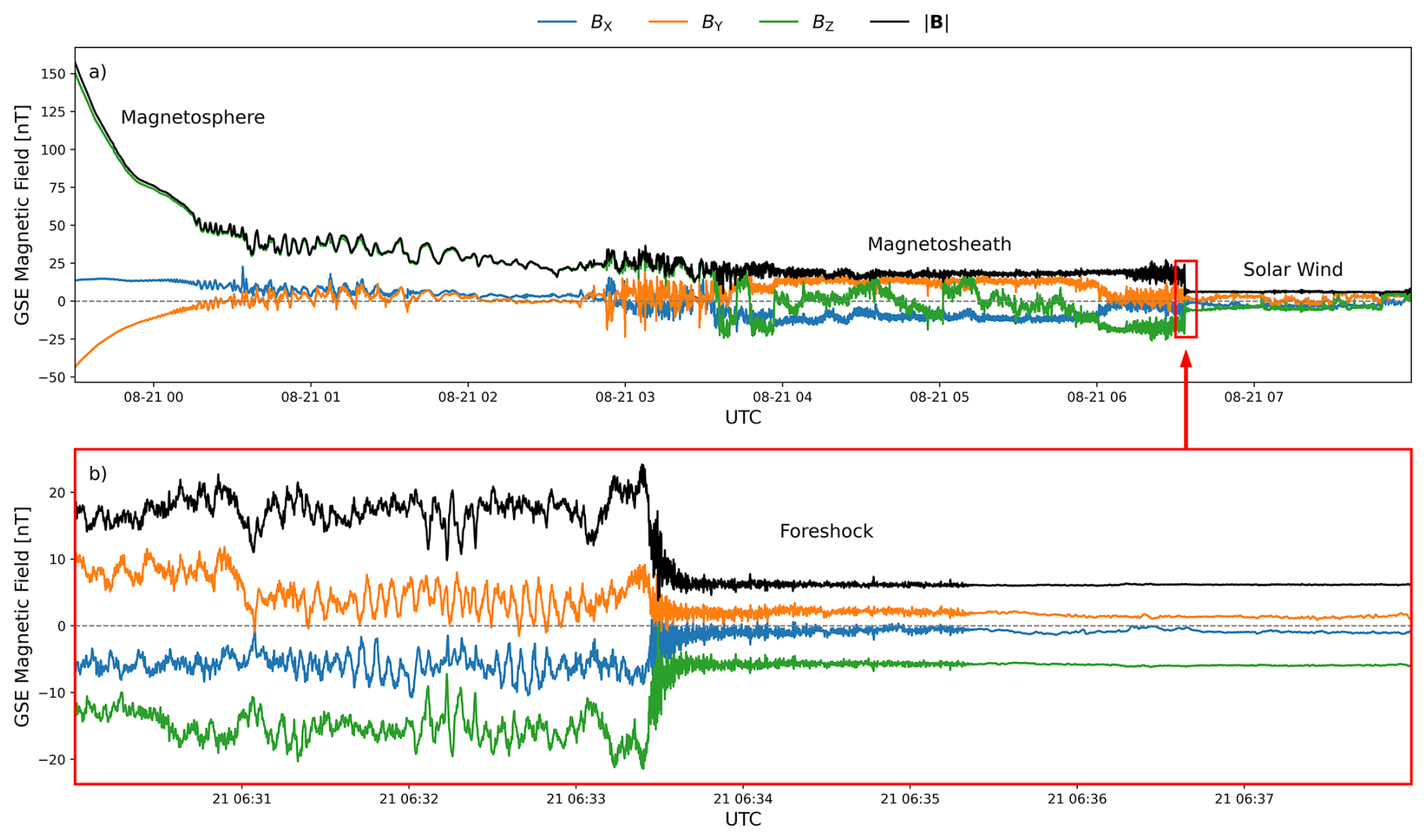
Figure 7 J-MAG magnetic field measurements (GSE) during magnetospheric exit on 21 August. Panel (a) shows the field vector and magnitude as the spacecraft transited the magnetosheath and entered the solar wind. Panel (b) shows a zoom of the bow shock crossing (red square in top panel).

Before leaving the magnetosphere, J-MAG saw significant field oscillations from around 00:15 until 02:30. These oscillations take place in a background field of around 40 nT (though gradually decreasing throughout), with amplitudes of order 10 nT and periods between 1–9 min, increasing with proximity to the magnetopause. Given these scales, it seems likely that these are MHD-scale ultra low frequency (ULF) oscillations (Pc5 band), perhaps associated with field line resonances (e.g. Chen and Hasegawa, 1974), global cavity modes (e.g. Kivelson and Southwood, 1985), or Kelvin Helmholtz instabilities (e.g. Southwood, 1968). The magnetopause crossing itself is poorly defined, with several possible partial crossings in quick succession (seen by field rotations, predominantly B_Z, at the current sheet boundary), and a possible pile-up layer. After this, Juice entered the magnetosheath. That is, a region of shocked, slowed, compressed solar wind. The field magnitude in this period is around 18 nT, though a degree of high-frequency fluctuations and occasional field rotations are seen. This is consistent with known properties of the turbulent magnetosheath (e.g. Zhang et al., 2019).

The bow shock crossing shown in Fig. 7b is much more abrupt than the magnetopause crossing, and shows the expected structure of a quasi-perpendicular shock with a foot, ramp, and overshoot (e.g. Bale et al., 2005). The shock-normal to interplanetary magnetic field angle is around 70°, calculated using the magnetic coplanarity theorem. Upstream of the shock, there is a short foreshock with high-frequency fluctuations, perhaps kinetic whistler waves (e.g. Zhang et al., 1998), lasting approximately 2 min for Juice's passage (from 06:33:30 to 06:35:20). This corresponds to around 440 km in space. Downstream of the shock (left side of plot) we see some evidence for mirror mode waves, which often can be seen in high β plasma downstream of perpendicular shocks and exhibit proportionally large fluctuations in $\left|\mathit{B}\right|$, though further investigation (including plasma moments) would be needed to confirm this.

While there is clearly a wealth of physical interest in this short interval, we do not explore it further in this paper, but note once again that this is an excellent demonstration of J-MAG's ability to observe such phenomena, which is very promising for future endeavours at Jupiter and Ganymede, where we expect to see comparable field magnitudes to some of the outer magnetospheric regions explored here.

Figure 8 shows J-MAG measurements (red) at a 1 min cadence over several days, after Juice exited the magnetosphere and was travelling duskward through the solar wind. Overlaid are corresponding measurements from the OMNI database (grey), sampled at L1 and propagated to Earth's bow shock, also at 1 min cadence. Note that these are the same data shown in the latter half of Fig. 2a.

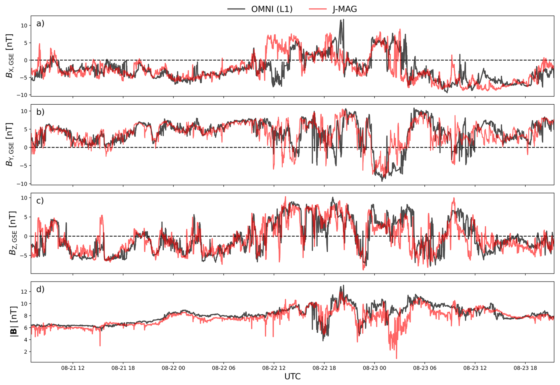
Figure 8 Comparison of J-MAG measurements (red) with those from OMNI (measured at L1 by Wind, grey), over several days in the solar wind after the LEGA. During this time, Juice moved around 120 R_E duskward from Earth. All field vectors shown in GSE coordinate system.

No timing adjustments have been made to either dataset to align the observations, though the OMNI data are inherently time-shifted and evolved from their L1 observation point to represent the conditions at Earth's bow shock nose. As discussed earlier (alongside Fig. 2), the bow shock X-position varied throughout this time interval according to the solar wind dynamic pressure. This variation (of order ∼3 R_E) is less than the movement of Juice over the same period, whose GSE X-position varied from 5 R_E to 14 R_E (from 9.5 R_E behind bow shock to 1 R_E ahead). At the average solar wind speed in this interval, this corresponds to a maximum difference in propagation time of approximately 3 min. We therefore conclude it is reasonable to expect solar wind evolution to be minimal between the bow shock and Juice X-positions. We note, however, that the propagation of Wind data to the bow shock covers around 200 R_E (∼60 min).

On large scales, the two datasets agree remarkably well, both in terms of absolute magnitudes and in vector fluctuations. This is another excellent validation of J-MAG's performance. We do see some notable differences on smaller scales, however, particularly towards the second half of the dataset, where there are several instances of rotational discontinuities seen by Juice but not captured by OMNI, and we notice that the alignment of observed structures also worsens. While the X-alignment of Juice and the bow shock generally improves throughout the interval (and so should improve temporal alignment), the displacement in Y_GSE increases significantly as Juice moves duskward of the Sun-Earth line (see Fig. 1). In addition, the Wind spacecraft, from which the OMNI data originate, was actually located dawnward of the Sun-Earth line. This means that the lateral displacement from Wind to Juice extended from 130 R_E to 250 R_E over this period. It is well-known that spatial structures in the solar wind can vary considerably on this scale (e.g. Borovsky, 2018), and so is unsurprising that the finer scale field structure differs more towards the end of the interval.

Despite these differences, there is a generally very good correspondence between the two datasets. This also demonstrates the potential utility of Juice (and other planetary missions) during cruise phase as solar wind monitors for the purposes of space weather forecasting, if the science payload is active and data can be transmitted to ground with low latency with a minimal (and fully automated) calibration applied. Though this calibration level would not be suitable for science studies, these low latency data may be useful for identifying and parametrising large events and geoeffective conditions, such as strongly negative B_Z. This has been successfully demonstrated with Solar Orbiter, where low-latency magnetometer data have been used for real-time predictions of CME arrival times and geoffectiveness when sunward of L1 (see, e.g. Laker et al., 2024), giving greater advance warning than current operational systems. We would argue that planetary missions should be used to the same end when in cruise phase, though this would require the science payload to be operational more often and for more extended periods than is typical at present.

Even if near-real time downlink is not possible, continuous operation during cruise would aid the reconstruction of solar wind transients and post-event analysis of space weather. The often unusual orbits of these missions during cruise can allow for sampling of regions of the heliosphere for which we do not have regular coverage. For example, observations at 1 AU but significantly away from the Sun-Earth line may provide useful training data for the development of the upcoming Vigil mission to the L5 Lagrange point (e.g. Eastwood et al., 2024). This extended coverage may also improve understanding of potential space weather hazards at other planets and spacecraft and, as is becoming increasingly relevant, conditions conducive for human spaceflight.

5 Summary and conclusions

In this paper, we have presented the first results from the Juice magnetometer during the Lunar-Earth gravity assist of August 2024. We have demonstrated the excellent performance of all three J-MAG sensors during this period, despite in-flight calibration being only preliminary at this stage in the mission. The operation of the scalar sensor in this environment proved challenging but was executed successfully. The flyby's interesting trajectory allowed for several opportunities to validate J-MAG observations against those from other spacecraft and models. During the lunar pass we compared J-MAG with ARTEMIS, seeing good agreement in the latter half of the short window. At the close approach to Earth, we used the IGRF-14 and Tsyganenko 2001 models to calculate an approximate value for sensor misalignment, finding it to be less than 1°, and seeing very good agreement with the predicted geomagnetic field. In the solar wind, we were able to compare J-MAG data with those measured at L1 (from OMNI), also finding excellent agreement despite increasingly large spatial separation. This showed the potential utility of using Juice as a solar wind monitor during the cruise phase, if the science payload is operational. We also highlighted several regions of interest for further study during magnetospheric exit, with the preliminary results proving promising for the Ganymede phase of the mission.

We have learned of several areas for future calibration activities and made suggestions for future operations. In order to improve calibration, stable temperatures are required, suggesting J-MAG should be switched on well in advance of encountering any body of interest. Temperature-dependent scaling can also be made when more flight data are available to study the effects. With more time operating in the solar wind, we can build up a better understanding of in-flight offset adjustments, and the two upcoming Earth flybys present further opportunities for alignment calibration. Part of this will also include operating the JACS, the study of which during the LEGA is ongoing. Future EGAs will also include opportunities to calibrate the fluxgate sensors against data from the scalar sensor. Finally, we hope that future EGAs will include a more extended operation of the in situ payload to allow for unprecedented opportunities to explore rarely-sampled regions of the magnetosphere, including the deep magnetotail. Overall, J-MAG performance during the LEGA was excellent, and we look forward to the next Earth gravity assist in September 2026.