Statistical properties of internal modulation in pulsating aurora

We statistically investigated the occurrence characteristics of internal modulation (IM), a rapid intensity modulation of a few hertz embedded in pulsating aurora (PsA), using high-speed ground-based optical data obtained with qCMOS cameras. For datasets acquired at Kiruna, Sweden, and Skibotn, Norway, we applied a two-step hierarchical machine-learning classification, first identifying the presence of PsA and then determining whether IM was present within the PsA. This enabled IM, which has previously been examined mainly through case studies, to be quantified for the first time in a systematic and statistically comparable manner. The results show that the fraction of PsA accompanied by IM increases toward the morning-sector magnetic local time (MLT) sector and tends to be higher at the lower-latitude site, Kiruna, than at the higher-latitude site, Skibotn. Representative examples from the classification results show that, on the midnight sector, IM commonly appears as a hierarchical structure superposed on clear main pulsations, whereas on the morning sector, the main pulsation tends to be relatively weak and the IM component often becomes dominant, suggesting that the morphology of IM itself also depends on MLT. These results suggest that IM is not merely an apparent subtype accompanying PsA, but rather a diagnostic feature that may provide insight into the wave–particle interaction underlying PsA.

1 Introduction

Pulsating aurora (PsA) is a form of diffuse aurora that occurs predominantly from midnight to the morning sector, mainly during the recovery phase of substorms (e.g., Brekke and Pettersen, 1971; Yamamoto, 1988; Partamies et al., 2017; Nishimura et al., 2020). PsA has long been recognized as a phenomenon in which irregular patchy structures brighten and dim in a quasi-periodic manner. Its temporal variation, however, is not characterized by a single period; instead, previous studies have reported a hierarchical structure in which rapid luminosity modulations of a few hertz are embedded within main pulsations lasting several to several tens of seconds (e.g., Royrvik and Davis, 1977; Nishiyama et al., 2014; Miyoshi et al., 2015b; Hosokawa et al., 2020). In this paper, we refer to these rapid modulations of a few hertz as internal modulation (IM), following previous studies.

The hierarchical modulation structure of PsA provides a valuable window into wave–particle interaction processes in the inner magnetosphere. In particular, pitch angle scattering of electrons by whistler-mode chorus waves has been established as a primary mechanism driving the electron precipitation responsible for PsA, based on in-situ satellite observations of chorus waves and conjugate ground-based optical observations (e.g., Nishimura et al., 2010; Kasahara et al., 2018; Hosokawa et al., 2020). More recently, a hierarchical correspondence has been increasingly supported by high-time-resolution ground-based optical observations and simultaneous satellite measurements: chorus bursts on timescales of seconds correspond to main pulsations, whereas individual chorus elements on subsecond timescales correspond to IM (Miyoshi et al., 2015b; Hosokawa et al., 2020; Ozaki et al., 2018, 2019; Nanjo et al., 2023; Chen et al., 2024). Miyoshi et al. (2015b) proposed a model in which the main pulsations are caused by chorus bursts, while IM is produced by chorus elements embedded within chorus bursts. The model is confirmed by a conjugate observation between the Arase satellite in the magnetosphere and ground-based observations (Hosokawa et al., 2020). These findings strengthen the idea that IM may directly reflect quasi-continuous scattering and precipitation driven by individual chorus elements such as rising tones, and suggest that observations and statistical characterization of IM can help constrain the temporal structure, propagation conditions, and resonant energy range of magnetospheric electrons.

On the other hand, studies of IM still remain limited by methodological constraints, although some broad characteristics, such as its more frequent occurrence on the morning sector, have been reported (Royrvik and Davis, 1977). First, because IM is a rapid modulation at frequencies of a few hertz, it cannot be directly examined with many cameras operating at cadences longer than 1 s, whereas high-time-resolution instruments such as photometers are limited in field of view. Second, image sampling rate is intrinsically traded off against signal-to-noise ratio (SNR), making it difficult to improve temporal resolution while retaining sufficient sensitivity to detect IM, whose amplitude is not large (Nishiyama et al., 2016). For reference, Royrvik and Davis (1977) reported that the amplitude of the 3 ± 1 Hz modulation could reach approximately 20 % in relative intensity. Third, statistical analysis of the large datasets produced by high-speed imaging requires automated methods capable of robustly labeling and classifying the datasets.

In recent years, automatic detection and classification of auroral images using deep learning have rapidly advanced as foundational techniques for both observational operations and statistical analysis (e.g., Kvammen et al., 2020; Nanjo et al., 2022; Partamies et al., 2024). However, existing automated classification has focused mainly on classifying images acquired at a single moment, and frameworks for statistically treating rapid temporal modulations of a few hertz, such as IM embedded within PsA, remain underdeveloped. Consequently, statistically characterizing the occurrence of IM as a function of MLT and magnetic latitude (MLAT) remains a largely unresolved challenge, despite its importance for constraining wave–particle interaction processes from ground-based observations.

To address this gap, we use ground-based optical observations obtained with state-of-the-art high-sensitivity, high-speed cameras to construct a hierarchical deep-learning model that takes keograms (plots produced by stacking pixel intensities along a fixed spatial slice over time) as input and systematically estimates (i) the presence or absence of PsA (main pulsations) and (ii) the presence or absence of IM conditional on the presence of PsA. We further aim to statistically evaluate the MLT dependence of the IM occurrence rate and its site-to-site difference by comparing two observation sites at different latitudes and similar longitudes. This allows IM research to move beyond case-study-based discussions toward a statistically comparable framework based on a clearly defined observational sample. Based on these results, we discuss several factors that may affect whether IM is visible in optical observations, including variations in the temporal structure and propagation of chorus waves.

2 Optical observations

2.1 qCMOS cameras

To resolve intensity modulations at frequencies of a few hertz, high-speed imaging is required. We used an ORCA-Quest quantitative CMOS (qCMOS) camera (Hamamatsu Photonics) equipped with a Kowa LM8HC lens (F1.4, f=8 mm). The camera was operated at 20 Hz, which satisfies the Nyquist criterion for the targeted modulation frequencies.

The native sensor format is 4096 × 2304 pixels; however, on-board hardware binning was applied to reduce the effective image size to 1024 × 576 pixels. The resulting field of view (FoV) is 76° in the horizontal direction. A BG3 glass filter (Samara et al., 2012) was placed in front of the lens to block the strong forbidden lines at 557.7 and 630.0 nm, while retaining sensitivity to the N${}_{\mathrm{2}}^{+}$ first negative and N₂ first positive band systems. This configuration was chosen to improve the SNR by emphasizing broadband auroral emissions rather than a specific emission line.

The same camera systems with the same optical configuration and acquisition settings were deployed at Kiruna, Sweden (67.841° N, 20.411° E), Abisko, Sweden (68.355° N, 18.819° E), and Skibotn, Norway (69.348° N, 20.363° E). The Abisko dataset is limited because the deployment started later than at the other sites. In addition, the FoV overlap between Kiruna and Abisko is substantial, which could lead to double counting of the same auroral structures in statistical analyses. Therefore, Abisko data are excluded from the statistics presented in this study, and we focus on observations from Kiruna and Skibotn. The Kiruna dataset used in this study covers October 2024 through December 2025, whereas the Skibotn dataset covers October 2023 through December 2025. These two sites are located at nearly the same longitude but at different latitudes, and their FoVs do not overlap when projected to an emission altitude of 100 km. Over the observation period, Kiruna and Skibotn correspond to AACGM latitudes (Shepherd, 2014) of approximately 65.1 and 66.7°, and L values of approximately 5.6 and 6.4, respectively, noting that magnetic coordinates are time dependent. The FoVs of the two sites projected to 100 km altitude are shown in Fig. 1.

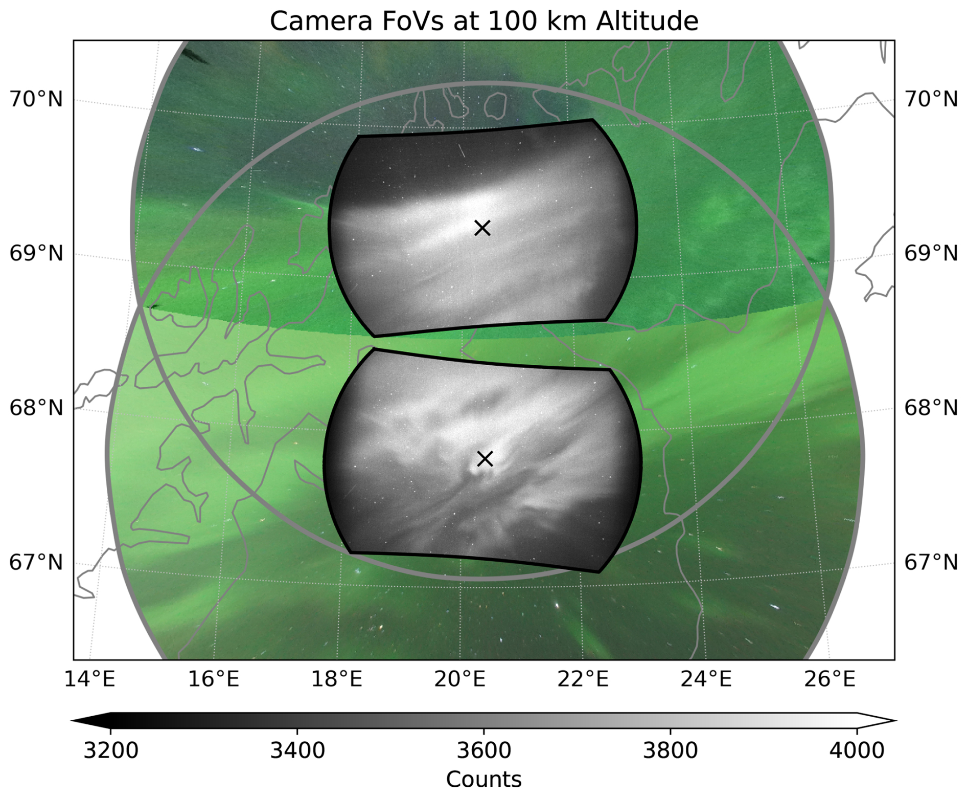
Figure 1 Fields of view of the qCMOS cameras and color all-sky cameras projected to an emission altitude of 100 km. The crosses mark the camera locations, with Skibotn, Norway, in the upper (northern) cross and Kiruna, Sweden, in the lower (southern) cross. The two sites are separated by approximately 170 km. The geometrical field of view of the qCMOS cameras calculated from the exact image size are wider in the east–west direction, but the outer part was cropped because of strong vignetting; the effective fields of view are outlined by the black lines. The background color image is a projection of simultaneous observations from the color all-sky cameras installed at the same sites. Only regions above an elevation angle of 20° (shown by the gray circles) are plotted. In areas where the fields of view overlap, the image with the higher elevation angle (and thus higher spatial resolution) is preferentially displayed. The images were obtained at 03:02 UT on 21 October 2025.

2.2 Color all-sky cameras

In addition to the qCMOS cameras, all-sky commercial digital cameras were operated at both Kiruna and Skibotn and used to provide complementary observations. In Kiruna, a Sony α7S equipped with a Nikkor 8 mm F2.8 lens was installed in the same building as the qCMOS camera; the camera was operated at ISO 4000 with an exposure time of 4–13 s, which was automatically adjusted depending on sky brightness. At Skibotn Observatory, a Sony α6400 with a MEIKE MK-6.5 mm F2.0 lens was used at ISO 8000 with an exposure time of 8 s. In Skibotn, the nominal imaging cadence is 1 min, but it can increase to 20 s when a near-real-time deep-learning image classifier detects auroral activity (Nanjo et al., 2022, 2026). These color all-sky images are used here for pre-selection of the data and to provide wider morphological context.

3 Machine learning detections

3.1 Training data and labeling

The presence or absence of IM was determined automatically from keograms using supervised image-classification models based on a ResNet-18 backbone (He et al., 2016) initialized with ImageNet-pretrained weights. As a pre-selection step, we used color all-sky camera images acquired at Kiruna and Skibotn. These images were independently classified for each site by the Tromsø AI system (Nanjo et al., 2022), which is based on a ResNet-50 backbone and outputs probabilities for eight classes: Arc, Discrete, Diffuse, Aurora but cloudy, Aurora but bright, Clear, Cloudy, and Dusk and Dawn. Model performance is reported in Nanjo et al. (2022), with an average precision of 93.1 % and an F1 score of 93.4 %. Here, the F1 score is defined as $F_{\mathrm{1}}=\mathrm{2}PR/(P+R)$, where P and R denote precision and recall, respectively.

To reduce computational cost, the Tromsø AI classifications were used only as a broad pre-screen for auroral activity. Minute-level intervals were retained when $p\left(\mathrm{Arc}\right)+p\left(\mathrm{Discrete}\right)+p\left(\mathrm{Diffuse}\right)\ge \mathrm{0.8}$ and the corresponding qCMOS data were available. This criterion was adopted because the color all-sky cameras and their acquisition settings differed between the two sites, and therefore the boundaries among the Arc, Discrete, and Diffuse classes may not have been identical. For each retained minute, we generated a 1 min keogram from the 20 Hz qCMOS image sequence. The keogram was constructed from a north–south slice through the image center, resulting in a size of 1200 pixels in the time direction and 576 pixels in the spatial direction.

The Tromsø AI output was not used to determine the presence of PsA or IM. The manually annotated intervals retained their human labels, whereas all the remaining intervals were evaluated using the hierarchical PsA–IM classifier described below. Thus, intervals pre-screened as Arc or Discrete could enter the initial sample, but they contributed to the denominator of p(IM∣PsA) only when they were subsequently classified as PsA-positive.

The above pre-screening procedure produced 30 464 keograms for Kiruna and 24 474 keograms for Skibotn, corresponding to 507.7 and 407.9 h of data, respectively. Although the nominal observation period was longer at Skibotn, fewer keograms were available because the availability of archived raw qCMOS data was intermittent. Major intervals during which all pre-screen-eligible minutes lacked corresponding raw data included 20–26 October 2023, 9–13 November 2023, 13–22 December 2023, 31 December 2023–5 January 2024, 9–16 September 2024, 31 December 2024–3 January 2025, and 4–6 March 2025. The Kiruna dataset consisted of 12 429 manually annotated keograms and 18 035 additional keograms evaluated by the model, whereas all 24 474 Skibotn keograms were evaluated by the model. For each keogram, MLT and MLAT were calculated using the geographic coordinates of the corresponding observation site and the observation time.

IM was detected using a two-stage hierarchical binary classification. First, a classifier determines whether a keogram contains PsA. Second, for keograms classified as containing PsA, a classifier determines whether IM is present. The definitions below were used to create supervised training labels for both stages. Because keograms are constructed over 1 min, we did not treat pulsations with repetition periods ≥ 30 s as PsA. IM was defined as the presence of intensity modulations at frequencies of a few hertz within keograms containing PsA. If both internally modulated and non-modulated patches coexist within a single keogram, the keogram was labeled as IM only when a majority of the pulsation patches exhibited IM.

Based on these definitions, we manually annotated 12 429 Kiruna keograms (98 nights) observed from October 2024 to September 2025. Of these, 243 keograms (2.0 %) were labeled as ambiguous (“?”) and excluded from model development, leaving 12 186 keograms for training/validation/testing. In this set, 8163 keograms from 90 nights were labeled as containing PsA (PsA = 1), and 2608 from 72 nights were labeled as containing IM within PsA (IM | PsA = 1).

Figure 2 shows representative examples of 1 min keograms used to illustrate the criteria adopted for creating the training labels, together with line plots extracted from selected horizontal bands in two of the keograms. Panels (a)–(c) are 1 min keograms constructed from a 20 Hz qCMOS image sequence. The horizontal axis represents time over the 1 min interval, while, in panels (a)–(c), the vertical axis shows pixel position along a north–south slice through the image center, with north at the top and south at the bottom, and grayscale indicates the raw count value. Panels (a') and (b') show the raw count values averaged over the narrow horizontal bands indicated by the dashed lines in panels (a) and (b), respectively. The title above panels (a), (b), and (c) gives the start and end times (UT) of the corresponding 1 min interval.

Figure 2a shows an example in which PsA is present but IM is not identified. Representative PsA structures without IM are indicated by the arrows. The corresponding line plot in Fig. 2a' shows relatively gradual intensity variations associated with the larger-scale patches, without clear modulations at frequencies of a few hertz. Figure 2b shows an example in which PsA is present and rapid intensity modulations (IM) are clearly embedded within its brighter phase. Representative regions in which IM is visible are indicated by the arrows. These rapid modulations are more clearly visible in the corresponding line plot in Fig. 2b'. In contrast, Fig. 2(c shows an example in which temporal variability is visible, but the morphology corresponds to flickering in discrete aurora; under the labeling scheme adopted in this study, it is therefore not classified as PsA. The arrow indicates a representative part of this discrete auroral structure.

Thus, Fig. 2 demonstrates that the labeling was not based simply on the presence or absence of temporal variation of any auroras, but instead distinguished between (i) the presence or absence of PsA and (ii) whether IM at frequencies of a few hertz was present when PsA was present. In particular, Fig. 2c shows that even when IM-like variation is visible, some events are excluded from PsA on the basis of their morphological context. This means that the training labels used in this study were defined not only by frequency-related features but also by morphological information.

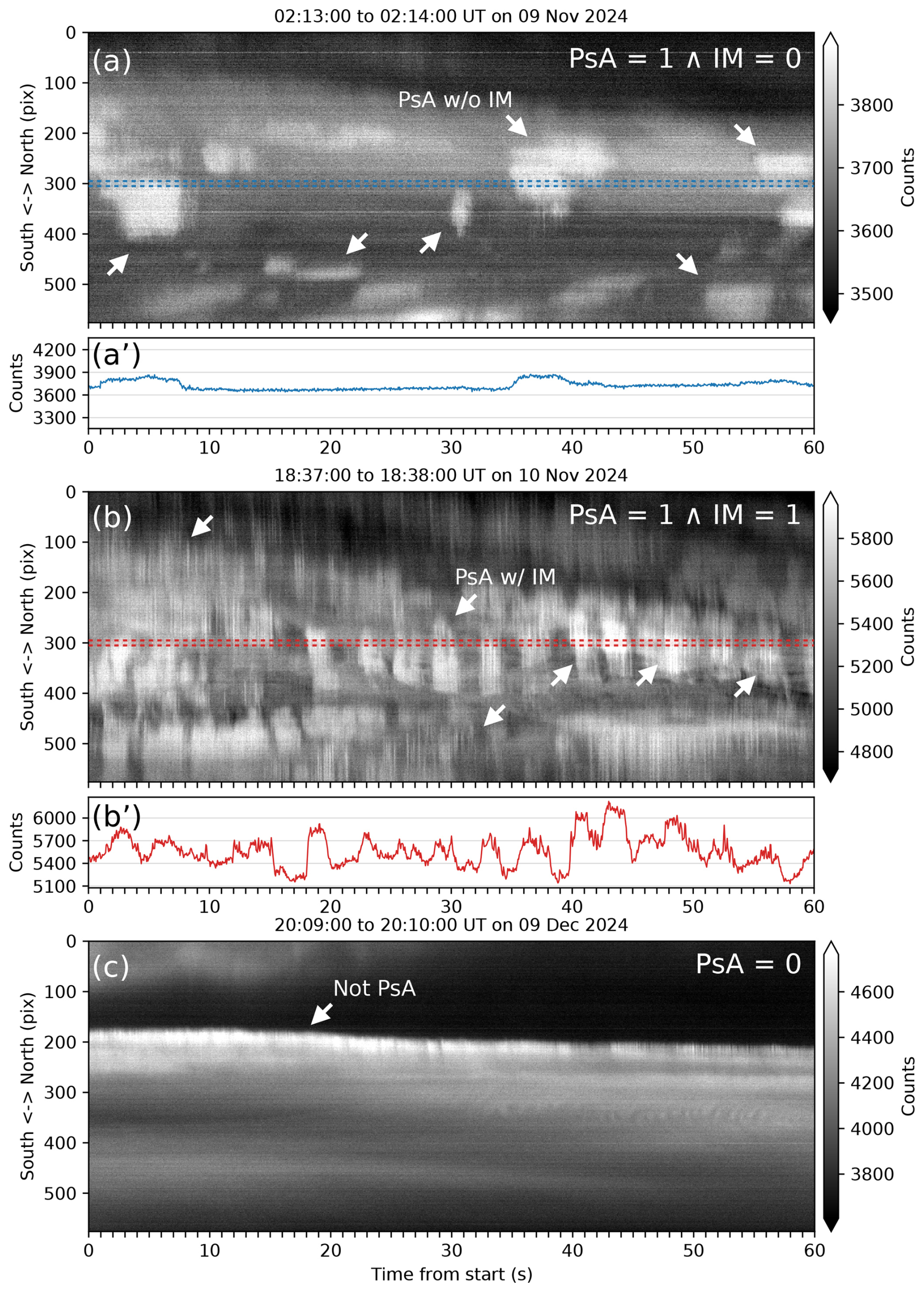
Figure 2 Representative examples of 1 min keograms used for labelling. Panels (a)–(c) show 1 min keograms constructed from a 20 Hz qCMOS image sequence. The horizontal axis represents time over the 1 min interval, while, in panels (a)–(c), the vertical axis shows pixel position along the north–south slice through the image center (top: north; bottom: south), and grayscale indicates the raw count value. The start and end times (UT) of the corresponding interval are shown above each keogram panel. (a) Example with PsA present and no IM. The dashed lines delimit the narrow horizontal band used to calculate the line plot in panel (a'). (b) Example with PsA present and IM present. The dashed lines delimit the band used to calculate the line plot in panel (b'). The line plots in panels (a') and (b') show the raw counts averaged over the respective bands. The same vertical span in counts is used in both line plots, allowing their modulation amplitudes to be compared directly. (c) Example without PsA; temporal variation is visible, but it corresponds to flickering in discrete aurora and is therefore not classified as PsA.

3.2 Model architecture and training

We used a hierarchical two-stage binary classification model that takes 1 min keograms as input. The first stage determines the presence or absence of PsA, and the second stage determines the presence or absence of IM conditional on PsA = 1. Hereafter, the performance of the first stage is denoted as PsA F1, and that of the second stage as IM | PsA F1. For the second stage, IM | PsA precision and IM | PsA recall were also evaluated.

The labeled keograms were split into training, validation, and test sets at the night level, such that keograms from the same night were never assigned to different subsets. This was done to avoid overly optimistic performance estimates caused by temporal correlation among neighboring keograms within a night. Here, an observing night was defined as the interval from 14:00 to 09:00 UT on the following day. For the fixed split used in the main analysis, the 98 nights were randomly assigned to the training, validation, and independent test sets, yielding 9398 keograms from 78 nights for training, 983 keograms from 10 nights for validation, and 1805 keograms from 10 nights for testing. The test set contained 1222 PsA-positive keograms from nine nights, including 432 keograms labeled as containing IM within PsA, also from nine nights. The test set was not used for model training, model selection, or early stopping and was used only for final performance evaluation.

Figure 3 summarizes the results of 10 training and evaluation runs performed under a fixed night split, with only the random seed varied. These 10 runs therefore share the same data split, and the differences among them mainly reflect variations arising from model initialization and training order. Accordingly, Fig. 3 is intended to assess reproducibility with respect to training randomness, rather than variability due to differences in data splitting. Variability associated with different night splits is examined separately in Appendix A.

Figure 3a shows the learning curves on the validation data. The thin pale lines indicate the curves for each of the 10 random seeds, whereas the thick lines indicate the run adopted for the analysis. Blue represents PsA F1 and red represents IM | PsA F1, and the red circle marks the epoch at which IM | PsA F1 reached its maximum in the adopted run (best epoch = 8). In this study, the validation IM | PsA F1 was used as the monitoring metric for model selection and early stopping. An epoch was regarded as an improvement only when this metric exceeded its value at the previous epoch, in which case the best model was updated. Training was stopped when the number of consecutive epochs without improvement reached four, and the test evaluation after training was always performed using the best epoch model rather than the weights from the final epoch. Therefore, the curves in the later epochs of Fig. 3a illustrate the behavior of the training process, whereas the test-performance values correspond to the best epoch selected on the basis of validation IM | PsA F1.

PsA F1 remains consistently high overall, with only small variation among random seeds. In contrast, IM | PsA F1 exhibits larger variability. This likely reflects the greater ambiguity of IM labeling: IM is a relatively subtle phenomenon with lower amplitude, and a keogram is labeled as IM-positive only when internally modulated PsAs are judged to occupy the majority of the pulsating structures, making the boundary less clear even for human inspection. Note that the maximum number of epochs shown in the figure is affected by the early-stopping criterion described above, and therefore fewer runs are shown in the later epochs.

Figure 3b shows the distribution of test performance across the same 10 random seeds. PsA F1 is high, with a mean of 0.9506 (SD = 0.0071), indicating stable performance across seeds. In contrast, IM | PsA F1 has a mean of 0.7472 (SD = 0.0201), and its precision and recall show relatively larger variation, with mean values of 0.6630 (SD = 0.0500) and 0.8630 (SD = 0.0407), respectively. In other words, although the precision–recall balance of IM classification can vary with random seed, the overall F1 remains within a relatively narrow performance range. The test performance of the adopted run (PsA F1 = 0.9401, IM | PsA F1 = 0.7460, IM | PsA precision = 0.6847, IM | PsA recall = 0.8194) falls within the distribution of the 10-seed results in all metrics, indicating that the selected run is not an exceptional one.

Figure 3b also includes reference values for the IM-related metrics based on a weighted evaluation derived from visual review of the test-set misclassifications (orange points). This supplementary evaluation was introduced to reflect the quality of the misclassifications, distinguishing between clear model errors, borderline cases, and cases in which the ground-truth label itself may deserve reconsideration, rather than relying solely on strict binary scoring. Specifically, all 241 IM misclassifications in the independent test set produced by the adopted model (163 false positives and 78 false negatives, distributed over nine nights) were visually inspected, and the misclassifications were grouped into three categories. Heavy cases were assigned a weight of 1.0 and represent clear model errors, for example when IM is evident throughout the keogram but the model predicts non-IM, or vice versa. Borderline cases were assigned a weight of 0.5 and represent examples near the labeling boundary that are difficult even for human inspection, such as cases with weak modulation or cases in which IM-positive and IM-negative structures appear in roughly equal proportions within the image. Label-questionable cases were assigned a weight of 0.25 and represent examples for which the ground-truth label itself may be open to revision, making it difficult to regard the model output as a clear failure. Recomputing IM | PsA precision, recall, and F1 using these weights yielded IM | PsA F1 = 0.8290, IM | PsA precision = 0.7629, and IM | PsA recall = 0.9077, all higher than the corresponding values from the standard binary evaluation (0.7460, 0.6847, and 0.8194, respectively). These results suggest that a non-negligible fraction of the IM misclassifications arises from cases near the definition boundary or from uncertainty in the reference labels.

Based on the above, we conclude that the model used in this study shows high reproducibility and stability for PsA detection. Although IM detection is accompanied by some uncertainty arising from boundary cases, its performance is sufficient for statistical analysis when interpreted together with the associated error assessment.

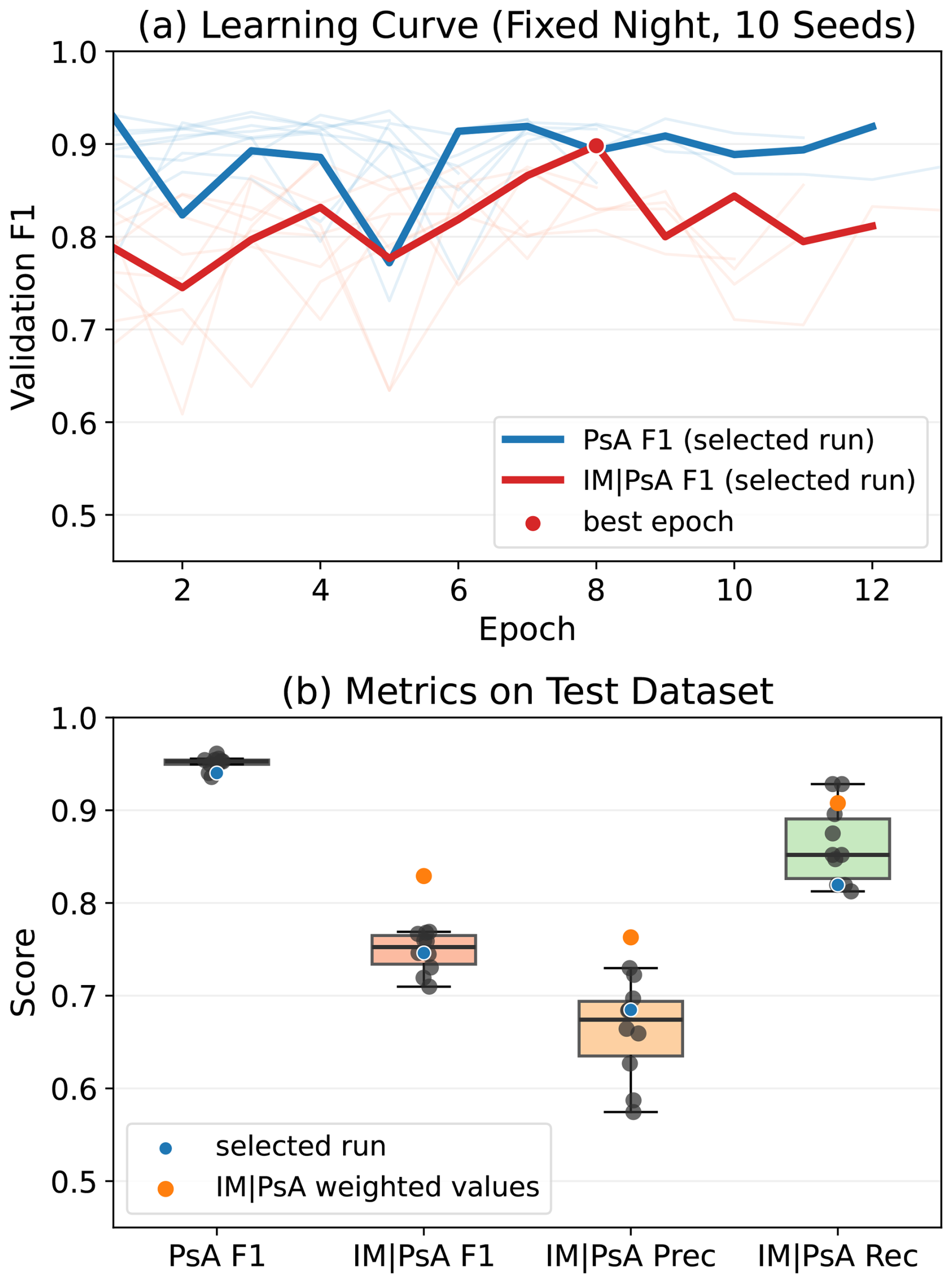
Figure 3 Summary of the training and test performance of the hierarchical two-stage classification model under a fixed night split. Results are shown for 10 runs with the night split fixed and only the random seed varied. (a) Learning curves on the validation data. Thin pale lines show the results for each random seed, and thick lines show the adopted run. Blue indicates PsA F1, and red indicates IM | PsA F1. The red circle marks the epoch at which IM | PsA F1 reaches its maximum in the adopted run (best epoch = 8). (b) Distribution of test metrics (PsA F1, IM | PsA F1, IM | PsA precision, and IM | PsA recall). The boxplots show the distribution across the 10 seeds, black points show the measured values for each seed, and the blue points indicate the adopted run. The orange points are reference values of weighted IM metrics based on visual review of the test misclassifications.

4 Results

4.1 MLT/MLAT dependence of IM occurrence

As shown in the previous section, PsA classification exhibited high reproducibility, and IM classification, although subject to some uncertainty arising from boundary cases, achieved performance sufficient for statistical analysis when interpreted together with the corresponding error assessment. We therefore applied the adopted model to unseen data to examine the MLT/MLAT dependence of IM occurrence. Figure 4 first summarizes the classification results in MLT bins, allowing comparison between the manual labels and model inference, as well as an overall assessment of site-to-site differences.

Figure 4 shows the number of 1 min keograms in each MLT bin, displayed as stacked bars for the categories $\mathrm{IM}=\mathrm{1}\wedge \mathrm{PsA}=\mathrm{1}$, $\mathrm{IM}=\mathrm{0}\wedge \mathrm{PsA}=\mathrm{1}$, and PsA=0 (with an additional “?” category in the manual labels for unclassifiable cases). Figure 4a shows the manual labels for Kiruna, Fig. 4b shows the model inference for unseen data from Kiruna, and Fig. 4c shows the model inference for unseen data from Skibotn. The model inference follows a hierarchical decision scheme: cases with p(PsA)≥0.5 are classified as PsA-positive, and for those classified as PsA-positive, cases with p(IM)≥0.5 are further classified as IM-positive.

This figure shows the number of images in each class, which is equivalent to the number of minutes because each image corresponds to a 1 min interval. The bar heights therefore directly reflect differences in sample size among the MLT bins. In particular, the earliest and latest MLT bins tend to contain fewer samples because the length of nights (dark time) varies seasonally, limiting coverage at those local times. Accordingly, the class composition should be interpreted together with the total sample size in each bin. In addition, whereas the manual labels include a reserved category for uncertain cases (“?”), the model outputs probabilities for all samples and therefore does not produce a “?” category.

Figure 4b and c also include count-based uncertainty estimates derived from the misclassification rates obtained from the test data, which is explained in Sect. 3.2. The black markers indicate ranges based on the uncorrected precision and recall (strict), shown as blue points in Fig. 3b, whereas the orange markers indicate weighted ranges that incorporate the visual review of IM misclassifications, shown as orange points in Fig. 3b. This allows the robustness of the observed trends to be assessed not only by direct comparison of bar heights, but also by taking classification errors into account. Specifically, for each MLT bin, let the model-predicted counts be denoted by N_IM for $\mathrm{IM}=\mathrm{1}\wedge \mathrm{PsA}=\mathrm{1}$, N_PsA for $\mathrm{IM}=\mathrm{0}\wedge \mathrm{PsA}=\mathrm{1}$, and N₀ for PsA=0. Asymmetric uncertainties were then assigned by applying the false-positive and false-negative rates derived from the test data, denoted by ϵ^FP and ϵ^FN, to the corresponding counts. For the top of the IM layer (the top of the red segment), we use

$$\begin{array}{}\text{(1)}& \mathrm{\Delta }{N}_{\mathrm{IM}}^{-}=N_{\mathrm{IM}}{\mathit{ϵ}}_{\mathrm{IM}}^{\mathrm{FP}},\mathrm{\Delta }{N}_{\mathrm{IM}}^{+}=N_{\mathrm{PsA}}{\mathit{ϵ}}_{\mathrm{IM}}^{\mathrm{FN}}.\end{array}$$

That is, the lower uncertainty is given by the IM false-positive rate, and the upper uncertainty by the IM false-negative rate. Furthermore, for the top of the PsA=1 layer (red + blue; shown only for the strict case), we define $N_{\mathrm{PsA}\mathrm{1}}=N_{\mathrm{IM}}+N_{\mathrm{PsA}}$ and use

$$\begin{array}{}\text{(2)}& \mathrm{\Delta }{N}_{\mathrm{PsA}\mathrm{1}}^{-}=N_{\mathrm{PsA}\mathrm{1}}{\mathit{ϵ}}_{\mathrm{PsA}}^{\mathrm{FP}},\mathrm{\Delta }{N}_{\mathrm{PsA}\mathrm{1}}^{+}=N_{\mathrm{0}}{\mathit{ϵ}}_{\mathrm{PsA}}^{\mathrm{FN}}.\end{array}$$

Accordingly, the markers in Fig. 4b and 4c do not represent statistical confidence intervals, but rather sensitivity-based uncertainty ranges in count space obtained by propagating misclassification rates to the observed counts.

Qualitatively, for Kiruna, the manual labels (Fig. 4a) and the model inference (Fig. 4b) share broadly consistent trends in the MLT-dependent changes in class composition. Note that the model-inference dataset for Kiruna (Fig. 4b) contains more samples than the manually labeled dataset (Fig. 4a), and therefore differences in total bar height partly reflect differences in sample size. Nevertheless, even taking this into account, both show a relative increase in the contribution of $\mathrm{IM}=\mathrm{1}\wedge \mathrm{PsA}=\mathrm{1}$ on the morning sector. In contrast, at Skibotn (Fig. 4c), even with the same model and decision criteria, the relative contribution of $\mathrm{IM}=\mathrm{0}\wedge \mathrm{PsA}=\mathrm{1}$ is larger than at Kiruna. This suggests that both physical differences between the regions sampled by the two sites and differences in observational conditions may influence the occurrence characteristics of IM. Overall, Fig. 4 demonstrates that the main trends identified from the manual labels are preserved, while the model inference enables expansion of the sample size.

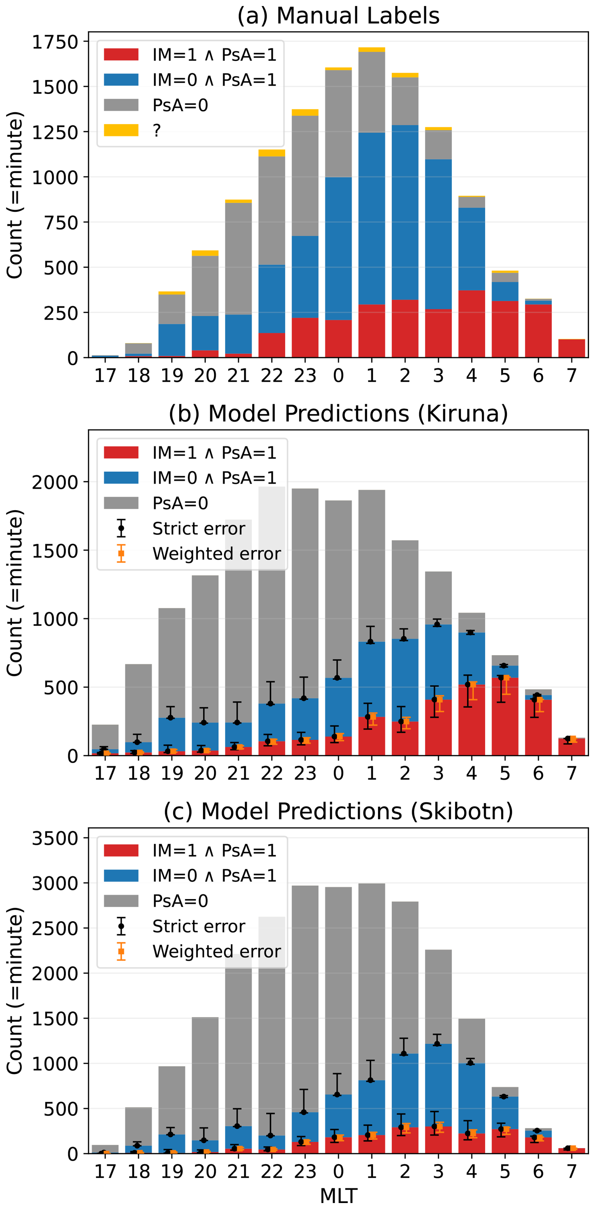
Figure 4 Stacked bar charts of classification results of 1 min keograms summarized by MLT bin, comparing (a) manual labels for Kiruna, (b) model inference for unseen data from Kiruna, and (c) model inference for unseen data from Skibotn. Each panel shows the number of keograms (Count = minutes) classified as IM = 1 ∧ PsA = 1 (red), IM = 0 ∧ PsA = 1 (blue), and PsA = 0 (gray; in the manual labels, an additional unclassified category “?” is shown in yellow). The error markers in panels (b) and (c) indicate count-based uncertainties derived from the test evaluation (black: strict; orange: weighted).

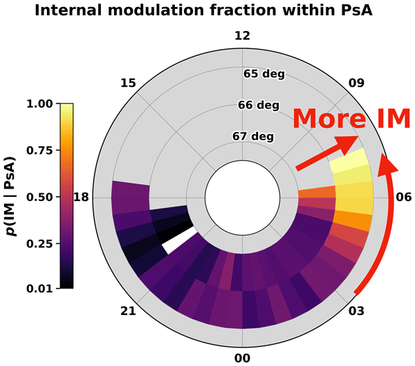
Figure 4 shows the classification counts in each MLT bin, but because the total number of samples (observing minutes) differs substantially among bins, the occurrence tendency of IM is better compared in terms of its fraction within PsA cases. Therefore, Fig. 5 compares the fraction of IM = 1 cases among PsA cases in each MLT bin (hereafter, the IM fraction within PsA) between Kiruna and Skibotn.

Figure 5a shows the IM fraction within PsA obtained by combining the manually labeled data and the model-inference data for Kiruna, whereas Fig. 5b shows the corresponding result derived solely from the model-inference data for Skibotn. Each bar represents the composition within cases classified as PsA=1, where the height of the red segment ($\mathrm{IM}=\mathrm{1}\wedge \mathrm{PsA}=\mathrm{1}$) corresponds to the IM fraction within PsA, and the blue segment ($\mathrm{IM}=\mathrm{0}\wedge \mathrm{PsA}=\mathrm{1}$) represents the remainder. Model classification was performed using the same hierarchical decision scheme as in Fig. 4 (first p(PsA)≥0.5, and then, for cases classified as PsA-positive, p(IM)≥0.5). MLT bins 17, 18, and 7 were excluded from this comparison due to the small number of samples and the resulting low stability of the ratio estimates. Across the MLT bins included in Fig. 5, the conditional ratios were calculated from 14 796 PsA-positive minutes at Kiruna and 7013 PsA-positive minutes at Skibotn.

The black (strict) and orange (weighted) error bars shown in the figure represent approximate uncertainties obtained by mapping the false-positive and false-negative rates of the IM classification into the ratio space. For Skibotn, uncertainties were propagated over the entire dataset because all keograms were classified by the model. In contrast, for Kiruna, the manually labeled portion was treated as fixed, and uncertainties were applied only to the model-inferred portion that was added. Therefore, the error bands for Kiruna primarily reflect the uncertainty associated with the model-derived component, rather than the uncertainty of the combined estimate as a whole. As a result, both sites show an increase in the IM fraction within PsA toward the morning-sector MLT. However, when compared at the same MLT, the values at Kiruna are higher than those at Skibotn in most bins, and this difference becomes more pronounced toward the morning sector.

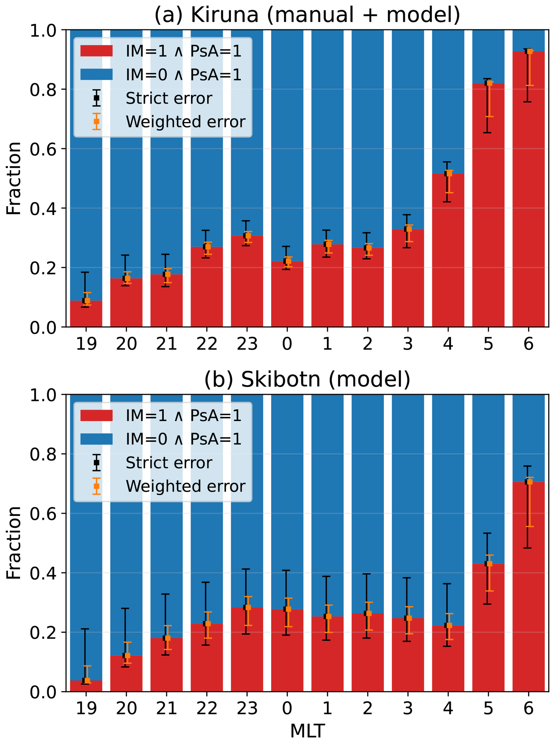
Figure 5 MLT dependence of the IM occurrence ratio $p(\mathrm{IM}\mid \mathrm{PsA}=\mathrm{1})$ for cases with PsA, compared between (a) Kiruna (combined manual labels and model inference) and (b) Skibotn (model inference only). In each MLT bin, the bars show the composition within PsA=1 (red: $\mathrm{IM}=\mathrm{1}\wedge \mathrm{PsA}=\mathrm{1}$; blue: $\mathrm{IM}=\mathrm{0}\wedge \mathrm{PsA}=\mathrm{1}$). Error bars indicate uncertainties derived by propagating classification errors using the FP/FN rates of the IM classification (black: strict; orange: weighted).

To make this difference more explicit, Fig. 6 shows the site-to-site comparison of the IM fraction (Kiruna − Skibotn) for each MLT bin. Positive values indicate that the IM fraction at Kiruna is higher than that at Skibotn at the same MLT. As in the previous figures, the black error bars indicate difference ranges based on the strict uncertainties, whereas the orange error bars indicate difference ranges based on the weighted uncertainties. The difference ranges were obtained by worst-case combination of the upper and lower bounds for Kiruna and Skibotn separately (lower bound = lower bound at Kiruna − upper bound at Skibotn; upper bound = upper bound at Kiruna − lower bound at Skibotn). The gray shading in the figure indicates MLT bins for which the strict uncertainty range does not include zero.

Figure 6 shows that, from the evening to midnight sector (19:00–03:00 MLT; MLT = 0 corresponds to approximately 22:00 UT), the site-to-site differences remained within the strict uncertainty ranges that include zero, and no significant difference was identified. In contrast, on the morning sector (04:00–06:00 MLT), the IM fraction at Kiruna was systematically higher, with central differences of 0.293, 0.390, and 0.221 at 04:00, 05:00, and 06:00 MLT, respectively. The corresponding strict ranges exclude zero at 04:00 MLT (0.058–0.403) and 05:00 MLT (0.120–0.541), whereas the strict range at 06:00 MLT (−0.002–0.452) marginally includes zero. Taken together, these results indicate that, in the morning sector, PsA was more likely to be accompanied by IM at the lower-latitude site (Kiruna) than at the higher-latitude (Skibotn).

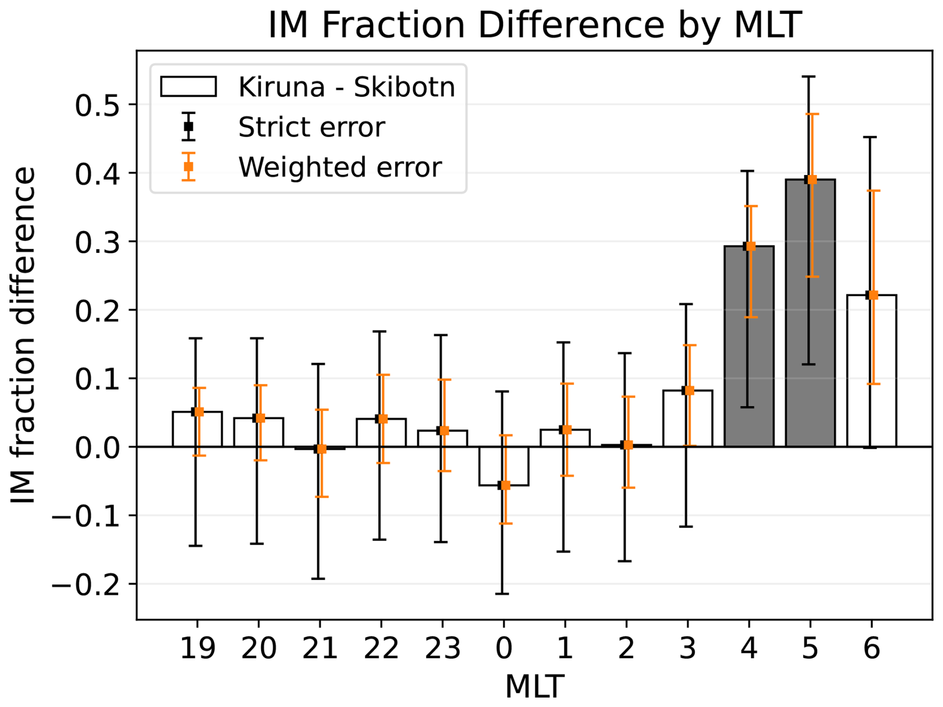
Figure 6 MLT dependence of the difference in IM fraction within PsA between Kiruna and Skibotn (Kiruna − Skibotn). The bars represent the central difference in each MLT bin. Error bars indicate difference ranges derived by propagating classification errors using the FP/FN rates of the IM classification (black: strict; orange: weighted). Gray shading marks bins for which the strict range does not include zero. On the midnight sector, the differences are small or the uncertainty ranges include zero, whereas on the morning sector (04:00–06:00 MLT), the values at Kiruna are systematically higher, with the strict ranges excluding zero at 04:00 and 05:00 MLT but marginally including zero at 06:00 MLT.

Figures 4–6 showed the MLT dependence of IM occurrence and its site-to-site (MLAT) dependence by summarizing the model classification results. In contrast, Fig. 7 shows a single-night example from evening to morning, with the keogram by the color all-sky camera and model probabilities displayed together to illustrate the tendencies seen in the statistical results at the event level. The example is from Kiruna and spans the evening of 20 November 2025 to the morning of 21 November 2025. The observations from this night were not used for model training. Figure 7a shows the keogram constructed from the color all-sky images. Figure 7b shows the probability of existence of PsA, p(PsA), and Fig. 7c shows the conditional probability of IM under PsA, p(IM∣PsA). Because the model probabilities were computed from keograms generated at 1 min intervals, the time resolution is 1 min. In addition, because the IM features were learned only from images containing PsA, p(IM∣PsA) is plotted as missing (NaN) at times when p(PsA)<0.5. This night was selected because auroral activity persisted throughout the night, allowing the evening-to-morning evolution to be illustrated continuously.

The keogram in Fig. 7a provides an overview of the temporal evolution of auroral activity during this night. Around 18:30 UT, discrete arcs appeared on the northern side, and from about 19:00 to 19:30 UT, structures propagating from north to south were observed. After that, faint diffuse aurora persisted for several hours. Around 21:40 UT, an auroral breakup was observed on the southern side, partly accompanied by red emissions suggestive of a contribution from the 630.0 nm OI line, and bright discrete aurora continued until around 23:00 UT. Thereafter, toward the morning sector, diffuse aurora again persisted until the dawn.

Comparing Fig. 7a with Fig. 7b and c, it can be seen that PsA appeared after both of two discrete auroras, whereas IM became prominent only after the latter discrete aurora (the auroral breakup). In addition, after the breakup, PsA maintained a high probability until the dawn, whereas p(IM∣PsA) showed more temporal variability. In other words, the IM probability did not remain constantly high: after an initial increase it decreased once, then rose again around 02:20 UT, and became more persistently elevated after about 02:50 UT.

The vertical dotted lines labeled A–D in the figure mark reference times on the keogram that are examined in Fig. 8 (A: 19:26 UT, B: 23:45 UT, C: 01:54 UT, D: 03:22 UT). At all of these times, p(PsA)=1.0, indicating strong support for the presence of PsA, whereas p(IM∣PsA) differs from one time to another. Specifically, it is low at A and C (A: 0.000, C: 0.002) and high at B and D (both 1.000).

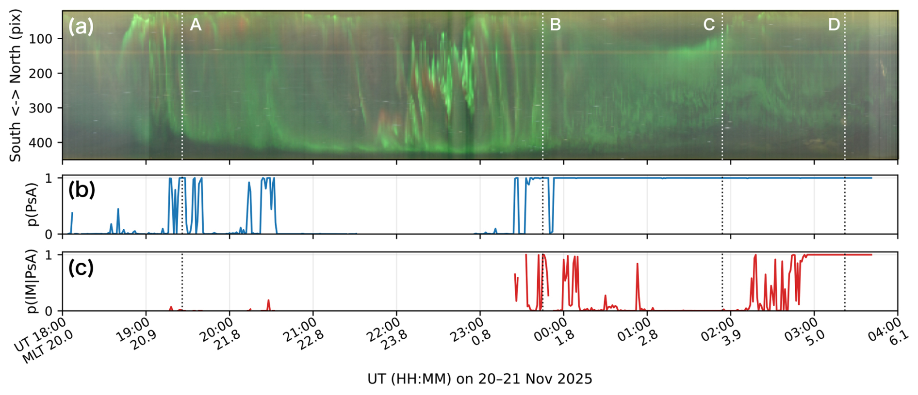
Figure 7 Simultaneous display of the keogram and model probabilities for a single-night event observed at Kiruna on 20–21 November 2025. (a) Keogram constructed from the color all-sky images, (b) probability of PsA, p(PsA), and (c) conditional probability of IM during PsA, p(IM∣PsA) with UT and MLT labels. The vertical dotted lines A–D mark representative times (A: 19:26 UT, B: 23:45 UT, C: 01:54 UT, D: 03:22 UT), which are examined in Fig. 8.

Figure 8 presents, for the representative times A–D shown in Fig. 7, the 1 min keograms from the qCMOS camera used as input to the model (left column) together with the corresponding color all-sky images from Kiruna, in which the qCMOS FoV is embedded (right column). This allows us to examine how the variations in the probability time series shown in Fig. 7 correspond to the actual data.

A (19:26 UT) corresponds to a case in which the model assigns a high probability to PsA and a low probability to IM (Fig. 7). In the qCMOS keogram (left), stable patches brighten and dim with a period of about 10 s, indicating clear main pulsations, whereas little IM is visible within them. In addition, in the patch region below the white dotted line, the background brightness remains higher than in the upper part even during the darker phases of the main pulsation, suggesting superposed background emission. In the color all-sky image, diffuse aurora dominates within the qCMOS FoV, and patch boundaries are not so clear in the single-frame image.

B (23:45 UT) corresponds to a case after the auroral breakup, for which the model assigns high probabilities to both PsA and IM. In the qCMOS keogram, as indicated by the white arrows, typical IM at about 2–3 Hz can be identified at multiple positions, embedded within the bright phase of the main pulsation. Although the main-pulsation period itself is comparable to that in A, there is a clear difference in morphology: in A, the brightening and dimming occurred relatively repeatedly at similar positions, whereas in B, the pulsating regions are distributed over multiple y positions (i.e., latitudes) within the FoV and appear spatially more unstable. As in A, the white dotted line indicates that background emission is superposed on the patch region (y-axis). In the color all-sky image, diffuse aurora is broadly distributed, with some patchy structures visible particularly on the lower-latitude side. Within the qCMOS FoV, a complex pattern is observed, and the patch boundaries are not very distinct.

C (01:54 UT) corresponds to a case in which the model assigns a high probability to PsA and a low probability to IM. In the qCMOS keogram, main pulsations are observed over a wider portion than in A and B, and the darker phase is shorter. In addition, as indicated by the white arrows, a few localized intensity modulations at around 1 Hz are present. However, unlike in B, these modulations appear as finer fragmentations of the main pulsation, rather than being clearly embedded within its bright phase. The background emission seen in A and B appears weaker in this case. In the right panel, the edges of patches are more clearly defined than in A and B, with a more distinct contrast between bright and dark regions.

D (03:22 UT) corresponds to a case in which the model assigns high probabilities to both PsA and IM, and the qCMOS keogram shows intensity modulations at about 1–2 Hz over a wide portion. Similar to the modulation seen in part of C, these fluctuations do not appear as modulations clearly embedded within the bright phase of the main pulsation. Rather, paradoxically given the terminology, the IM component itself appears to be dominant. In addition, the overall brightness during this interval was lower than in A–C (see the difference in color scale). The right panel shows an overall faint emission state, although some localized patch-like boundaries are still visible.

Overall, the comparison between the qCMOS keograms and the snapshot images in Fig. 8 shows that the model outputs in Fig. 7 (the time series of PsA/IM probabilities) are broadly consistent with the visually identifiable temporal structures, at least for this example. In other words, the model reasonably distinguishes intervals dominated by PsA from those in which IM is prominent. At the same time, even within events classified as the same PsA or IM category, there is clear diversity in the spatial structure of patches, the degree of background emission, the manner in which main pulsations and IM are superposed, and the overall brightness.

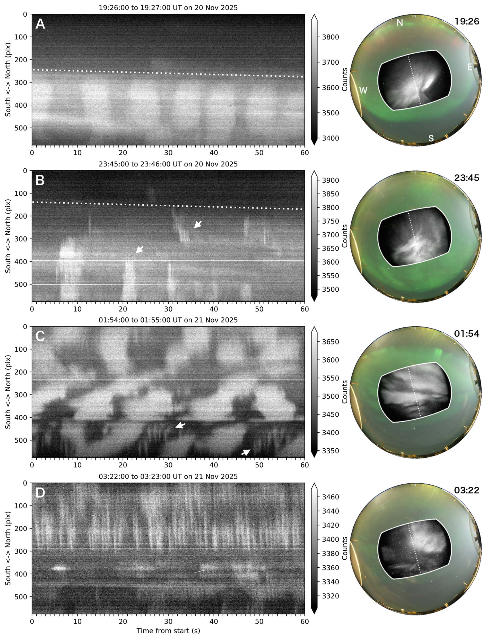
Figure 8 Comparison between the 1 min qCMOS keograms (left column) and the corresponding color all-sky images at Kiruna with the qCMOS FoV embedded (right column) for the representative times A–D in Fig. 7. Each row corresponds to A–D in Fig. 7 (A: 19:26 UT, B: 23:45 UT, C: 01:54 UT, D: 03:22 UT). The dotted line in the central part of the qCMOS image in the right panels indicates the slice used to construct the keogram. The qCMOS images embedded in the all-sky images share the same color scale as the keograms.

5 Discussion

We applied hierarchical machine-learning classification to qCMOS high-speed imaging data and, for the first time, investigated the occurrence characteristics of pulsating aurora (PsA) accompanied by internal modulation (IM) in a statistical and quantitative manner. As shown in Fig. 5, the IM fraction within PsA depends on MLT and increases toward the morning sector. Furthermore, Fig. 6 shows that, within this overall morning-sector enhancement, the lower-latitude site, Kiruna (MLAT of 65.1° and L=5.6), generally exhibits a higher IM fraction than Skibotn (MLAT of 66.7° and L=6.4). According to Figs. 3 and A1, the absolute occurrence rates vary to some extent depending on model initialization and data splitting; nevertheless, the two main tendencies remain evident: the IM fraction increases toward the morning sector, and, within the morning sector, it is higher at the lower-latitude site, Kiruna, than at Skibotn. The weighted sensitivity ranges for the site-to-site difference do not include zero at 04:00–06:00 MLT. Potential observational biases affecting these results are described in Appendix B.

One possible geometrical explanation for the higher IM fraction at the lower-latitude site, Kiruna, is that the two sites systematically sampled different parts of the auroral oval. Although their MLATs differ by only approximately 1.6°, previous observations have shown that the occurrence distributions of different PsA morphologies can vary over a comparable latitudinal scale. In particular, Grono and Donovan (2020) found that the occurrence peak of amorphous pulsating aurora was located approximately 1–2° MLAT poleward of those of patchy pulsating aurora and patchy aurora. Thus, the MLAT separation between Kiruna and Skibotn is sufficiently large for the two sites to sample regions of the auroral oval characterized by different PsA properties. The specific portions of the auroral oval sampled by each site vary with time as the position and shape of the oval evolve. Nevertheless, the relative geometry remains unchanged: Kiruna is consistently located at a lower MLAT than Skibotn. This persistent latitudinal separation may therefore introduce a systematic tendency for the two sites to sample regions with different characteristics, such as morphology or precipitation regime, which could in turn contribute to the observed difference in IM fraction. In light of the analysis presented in Appendix B, the site-to-site difference is difficult to explain solely in terms of observational biases. Therefore, the enhanced IM fraction at Kiruna, particularly around 04:00–05:00 MLT, should be interpreted as a robust site-to-site difference associated with MLAT.

In the example shown in Figs. 7 and 8, IM does not increase monotonically after the substorm. Instead, it first appears immediately after the disappearance of discrete aurora as modulation embedded within the main pulsation, then is followed by a period in which the main pulsation dominates, and later becomes prominent again as an IM-dominant state without a clear main pulsation. At least in this case, the occurrence of IM is non-monotonic in the substorm cycle, and its morphology can change over time.

The hierarchical periodic structure of PsA, consisting of main pulsations and IM, is known to have a clear correspondence with chorus waves. Recent high-speed ground-based observations together with conjugate satellite measurements have shown that these two levels of variation correspond, respectively, to chorus bursts and to the discrete chorus elements (rising tones) embedded within them in the inner magnetosphere (e.g., Hosokawa et al., 2020; Chen et al., 2024). It is therefore natural to interpret the IM identified in this study as the ionospheric projection of the occurrence of fine-scale chorus elements in the inner magnetosphere as shown by Miyoshi et al. (2015b). In this sense, statistical biases in IM occurrence may reflect differences in the presence or repetition timescale of chorus elements. Taken together, Hosokawa et al. (2020) and Nanjo et al. (2023) suggest that main pulsations correspond either to cases in which the repetition of chorus elements is indistinct or to cases in which they occur densely at frequencies around 6 Hz, whereas IM corresponds to cases in which the repetition of chorus elements is sparser, at around 3 Hz. Furthermore, Nanjo et al. (2023), based on conjugate observations with the Arase satellite, showed that such intervals were associated with decreases in hot-electron density and temperature anisotropy, suggesting that the presence or absence of IM may provide a way to discuss differences in the magnetospheric plasma environment involved in chorus-wave excitation. However, because the present study does not directly observe waves or particles in the magnetosphere, IM cannot be regarded as a unique diagnostic of those processes. Rather, it should be interpreted as a proxy that indirectly reflects differences in chorus-wave characteristics through ground-based optical observations.

The increase in the IM fraction toward the morning sector shown in Figs. 5 and 6, which is found at both sites, suggests that the excitation conditions and temporal structure of chorus waves depend on MLT. According to the nonlinear growth theory of chorus waves proposed by Omura (2021), the ease of chorus excitation (the threshold amplitude of waves) depends on the density and temperature anisotropy of energetic electrons, and Arase observations analyzed by Chen et al. (2025) demonstrated that energetic electron injection during substorms lowers the threshold amplitude and facilitates chorus excitation. In contrast, Nanjo et al. (2023) discussed a later stage after particle injection, in which hot-electron density and temperature anisotropy begin to decrease with time, increasing the threshold amplitude and making chorus less likely to occur continuously. Under such conditions, chorus may shift to a regime in which it appears more sparsely in time, allowing IM to become more prominent. The morning-sector MLT sector is geographically separated from the typical substorm onset region (around 23:00 MLT) (e.g., Frey et al., 2004), and the plasma parameters relevant to chorus excitation there may therefore evolve differently from those on the midnight sector because electrons injected from the magnetotail may lose energy through processes such as pitch-angle scattering before reaching that sector. This morning-sector enhancement may reflect spatial inhomogeneity in the post-substorm magnetospheric plasma environment. If the plasma conditions controlling chorus excitation evolve differently with MLT, the temporal spacing of chorus elements may also differ with MLT. The observed MLT dependence of IM occurrence may then arise as an ionospheric manifestation of that difference.

The above interpretation concerns differences in plasma parameters related to chorus generation. A separate, though complementary, aspect is propagation-related control on the energy range and time-of-flight (TOF) structure of the precipitating electrons, which may be relevant to at least some IM-dominant cases observed on the morning sector. As in Fig. 8D, some morning-sector cases show IM dominance without a clear main pulsation and with relatively low overall brightness. Such characteristics are consistent with a situation in which the energy (or velocity) dispersion of electrons interacting with an individual chorus element is small. In that case, the PsA emission associated with each chorus element would be expected to have a shorter duration, making the main-pulsation envelope less distinct than under conditions with larger TOF distributions. Miyoshi et al. (2020) showed that chorus waves propagating off the magnetic equator can produce precipitation of high-energy electrons with small velocity dispersion. This interpretation is also broadly consistent with statistical chorus distributions: Meredith et al. (2020) showed that, during active conditions, strong lower-band chorus extends up to $\left|{\mathit{\lambda }}_m\right|\sim \mathrm{18}\mathit{°}$ predominantly in the prenoon sector, typically over $\mathrm{5}<L<\mathrm{8}$, whereas on the nightside strong waves are largely confined to lower latitudes except for limited postmidnight low-L regions. Such a distribution supports the idea that propagation-related effects of chorus waves may become more important from the morning sector toward prenoon. If the velocity dispersion is limited, the total flux of precipitating electrons scattered by an individual chorus element would also be expected to be relatively small, likewise consistent with the low overall brightness seen in Fig. 8D.

One possible mechanism that may realize such high-latitude propagation is duct propagation of chorus waves along the field line (e.g., Smith et al., 1960; Angerami, 1970; Yearby et al., 2011). Ito et al. (2024) reported that patchy PsA, corresponding to high-energy electron precipitation, appeared during an interval for which duct propagation was suggested. In the present study as well, patch-like structures are seen in both Fig. 8C and D, although they are more clearly defined in Fig. 8C. This suggests that duct propagation may contribute to the formation of spatially coherent patchy precipitation. However, the optical visibility of IM does not by itself imply that duct propagation is required. Instead, IM may be more directly related to precipitation of relatively high-energy electrons with small velocity dispersion, whereas duct propagation, if present, may act only as one possible factor that facilitates off-equator propagation of chorus waves.

Consistent with this propagation-related interpretation, previous studies have suggested that the characteristic energy of electrons responsible for PsA tends to be higher on the morning sector (e.g., Hosokawa and Ogawa, 2015; Kawamura et al., 2020; Miyoshi et al., 2015a; Nanjo et al., 2021; Cessateur et al., 2026). In line with this picture, PsA has also been reported in some cases to occur simultaneously with sub-relativistic/relativistic electron microbursts (e.g., Kawamura et al., 2021; Namekawa et al., 2023; Shumko et al., 2023). In particular, Shumko et al. (2021) found a strong correlation between patchy aurora and >1 MeV electron microbursts during a conjunction between SAMPEX and a THEMIS all-sky imager. However, because the cadence of the optical observations was insufficient to resolve modulations at a few hertz, it remains unknown whether the aurora associated with those microbursts exhibited IM. Douma et al. (2017) reported that relativistic microbursts frequently occur at 04:00–11:00 MLT and L=4.5–6.0. Given that the L values of Skibotn and Kiruna are 6.4 and 5.6, respectively, these MLT–L characteristics are broadly consistent with the region where the IM fraction was high in the present study, namely 04:00 MLT and later at Kiruna.

The possible relationship between IM and microbursts also has implications for radiation-belt electron loss. Elliott et al. (2022) used multipoint observations of chorus waves and energetic-electron precipitation to constrain the spatial extent and approximately 30 h duration of a microburst-producing chorus region, and concluded that microbursts likely represented a major loss process for outer-radiation-belt electrons during that event. If IM is, in at least some cases, an optical signature associated with the high-energy tail of PsA precipitation, the statistical occurrence characteristics reported here may provide ground-based constraints on when and where such energetic precipitation is favored. However, because the present study is based solely on optical observations, the IM-dominant cases on the morning sector cannot be identified as relativistic electron microbursts themselves. The present results suggest only that, in at least some cases, relatively high-energy electron precipitation may have been involved. Coordinated observations with low-Earth-orbit particle measurements, including existing ELFIN observations and measurements from the recently launched REAL CubeSat, could test the relationship between optical IM signatures and the energy, pitch-angle distribution, and temporal structure of microburst precipitation.

The morphology of IM also appears to vary with MLT, as seen in Fig. 8B and D. Of course, these examples cannot be regarded as uniquely representative of midnight-sector and morning-sector IM, respectively, and in reality their characteristics overlap to some extent. Even so, on the midnight sector, cases like Fig. 8B, in which IM is embedded within a clearly defined main pulsation, were common, whereas on the morning sector, cases were often seen in which the main-pulsation component was relatively weak and the IM component appeared to dominate. In other words, although the typical hierarchical periodic structure was clear on the midnight sector, a substantial number of morning-sector cases appeared to show a breakdown of that hierarchy. A visual review of the 410 IM-positive keograms in the test set, excluding cases with unclear morphology, showed that the fraction in which the main pulsation was indistinct while IM remained clear was 36 % at 19:00–01:00 MLT and 69 % at 04:00–06:00 MLT. This suggests that the hierarchical time structure of the corresponding chorus waves may also differ with MLT. If multiple chorus elements are grouped together to form a chorus burst corresponding to the main pulsation, the burst-like periodicity may be relatively well preserved on the midnight sector, whereas on the morning sector the darker phase may become less distinct, with the elements appearing more continuously. Although chorus itself is already known to be more active from the morning sector toward the dayside (e.g., Li et al., 2011; Meredith et al., 2012), the MLT dependence of its burst periodicity and hierarchical temporal structure remains poorly understood. The present results may therefore provide a new observational constraint on theoretical and modeling studies of whistler-mode chorus generation and modulation. At the same time, this point is at present derived from optical characteristics, and it will be necessary in future work to test it through statistical analyses of in-situ observations.

As discussed above, the MLT/MLAT dependence of IM obtained in this study suggests that the spatiotemporal characteristics of chorus-related electron precipitation are not uniform. Because this study is based on statistical analysis of ground-based optical observations, it cannot uniquely identify the underlying plasma mechanisms or separate intrinsic MLAT dependence from differences in auroral-oval geometry and observational conditions. Nevertheless, by quantifying the occurrence tendency of PsA accompanied by IM, this study provides a new observational constraint on the MLT/MLAT dependence of chorus-wave generation, propagation, and the associated electron scattering.

6 Conclusions

In this study, we used high-speed imaging data from qCMOS cameras together with hierarchical machine-learning classification to statistically investigate, for the first time, the occurrence characteristics of internal modulation (IM) in pulsating aurora (PsA). The results show that the fraction of PsA accompanied by IM depends on MLT and increases toward the morning sector at both sites, and that, at the same MLT, the fraction is generally higher at the lower-latitude site, Kiruna. The site-to-site difference is most evident at 04:00–06:00 MLT, where the weighted sensitivity ranges exclude zero. The observational-bias analysis in Appendix B shows that the difference in IM fraction remains after accounting for observable exposure and PsA occurrence. These results support an MLAT dependence of IM occurrence, with a higher IM fraction at the lower-latitude site in the morning sector. Although residual contributions from weather and differences in the portions of the auroral oval sampled by the two sites cannot be completely excluded, they do not alter the main statistical result.

Event-based analysis further suggests that, on the midnight sector, typical hierarchical structures with IM embedded within clear main pulsations are common, whereas on the morning sector, cases are also observed in which the main-pulsation component is weak and IM becomes dominant. This implies that the morphology of IM itself may depend on MLT.

These results demonstrate the novelty of this study in treating IM, which has previously been addressed mainly through individual case studies, as a statistical and quantifiable phenomenon, and in revealing its MLT and MLAT dependence. IM may serve as a proxy for the spatiotemporal characteristics of chorus-related electron precipitation within PsA, and thus provides a new observational constraint for understanding the interaction between chorus waves and electrons.

Appendix A: Sensitivity of model performance to random night split

To complement Fig. 3, Fig. A1 summarizes an additional set of 10 training runs in which the night-level train/validation/test split was varied, while the model initialization seed was fixed. Whereas Fig. 3 isolates the effect of training stochasticity under a fixed night split, Fig. A1 evaluates how sensitive the model performance is to the particular assignment of nights to each subset.

Figure A1a shows the validation learning curves for these random-split runs. The spread among runs is larger than in the fixed-split case, especially for IM | PsA F1, indicating that the composition of nights in the training and evaluation sets affects the difficulty of the IM classification more strongly than the randomness of model initialization alone.

Figure A1b shows the distribution of the test metrics across the 10 random-split runs. The mean test scores were 0.933 for PsA F1 and 0.755 for IM | PsA F1, with standard deviations of 0.024 and 0.053, respectively. IM | PsA precision and recall also showed broader variation (means of 0.753 and 0.779; standard deviations of 0.090 and 0.110). Thus, the absolute performance depends to some extent on how nights are divided, but the overall performance level remains comparable to that obtained for the fixed-split experiment. This supports the robustness of the hierarchical classifier for the statistical analysis presented in the main text.

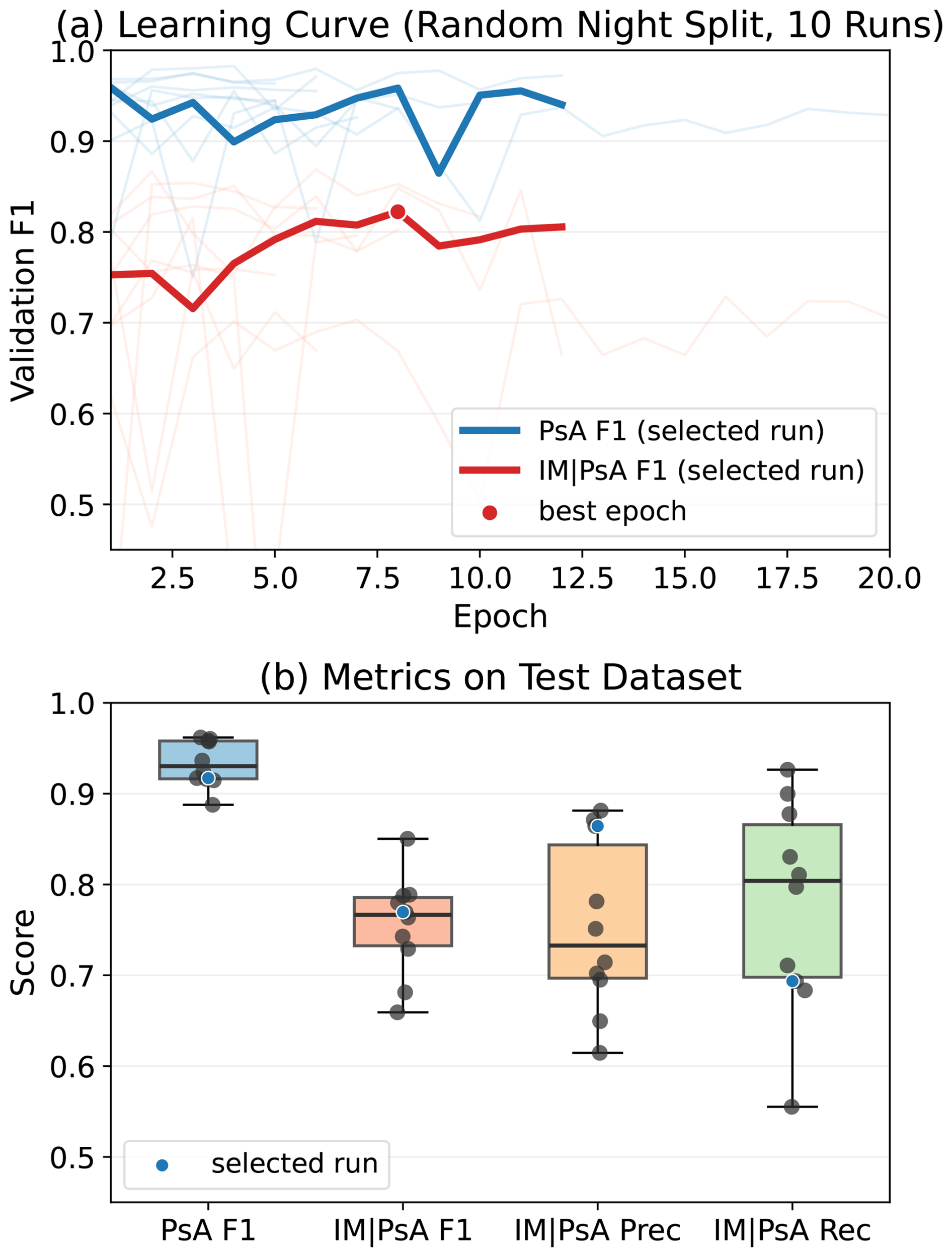
Figure A1 Summary of the hierarchical two-stage classification model for 10 runs with random night-level train/validation/test splits. (a) Validation learning curves. Thin pale lines indicate individual runs, and thick lines indicate a representative run. Blue shows PsA F1 and red shows IM | PsA F1. The red circle marks the epoch at which the validation IM | PsA F1 reached its maximum for the representative run. (b) Distribution of test metrics across the 10 random-split runs. Boxplots show the run-to-run distribution, black dots show individual runs, and blue dots indicate the representative run.

Appendix B: Observational biases in the MLT/MLAT dependence of IM

At both sites, IM occurred more frequently in the morning sector, and comparison between the two sites showed that the occurrence fraction of IM during PsA was higher at the lower-latitude site, Kiruna. One observational bias that could affect the robustness of these results is the presence of gaps in the qCMOS observations at Skibotn, as described in Sect. 3.1. If the observations had been continuous, the number of keograms at Skibotn would have increased to 37 672, exceeding the 30 464 keograms at Kiruna. Thus, the observational gaps constitute a major reason for the smaller number of images obtained at Skibotn. However, these gaps occurred intermittently in various months and typically persisted for several consecutive days rather than being confined to particular UTs. Therefore, they are unlikely to substantially distort statistical trends such as the MLT dependence. Figure B1a shows, for the analysis period of this study, the total observing time during which conditions suitable for auroral observations were satisfied, namely, when the sum of the occurrence probabilities for Arc, Discrete, Diffuse, and Clear from the Tromsø AI model exceeded 0.8 and qCMOS raw data were available. Although the observing time is shorter for the higher-latitude ring (Skibotn) than for the lower-latitude ring (Kiruna), no unnatural gaps or asymmetries are evident in the MLT distribution.

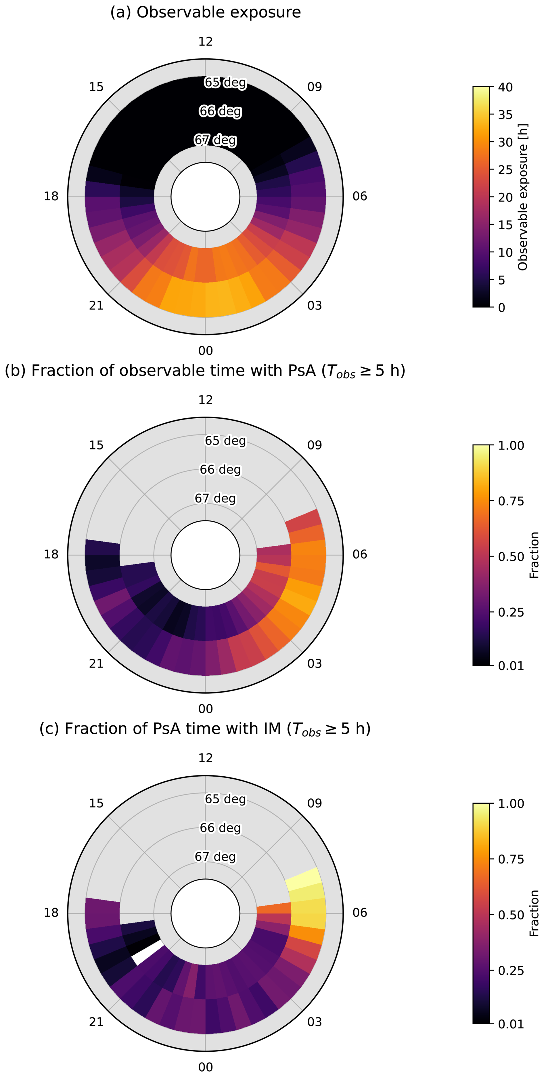
Figure B1 MLT–MLAT distributions of (a) observable exposure, (b) the fraction of observable time classified as PsA, and (c) the fraction of PsA time classified as IM at Kiruna and Skibotn. Panels (b) and (c) show only bins with at least 5 h of observable exposure.

Another observational bias that could contribute to the difference in observable exposure between Skibotn and Kiruna is the pre-screening based on the color all-sky cameras. Even when considering only periods for which qCMOS data were available at both Kiruna and Skibotn, the total duration that passed the pre-screening ($p\left(\mathrm{Arc}\right)+p\left(\mathrm{Discrete}\right)+p\left(\mathrm{Diffuse}\right)>\mathrm{0.8}$) and was included in the analysis was 16 398 min at Kiruna and 10 716 min at Skibotn, corresponding to 34.7 % less observing time at Skibotn. One possible reason is that the type of color all-sky digital camera and the sensitivity settings differed between the two sites, which could affect the sensitivity of the pre-screening procedure. Indeed, when the analysis is restricted to periods when the Moon was below the horizon at both sites or the lunar age was less than 3 d, the durations passing the pre-screening become 13 866 min at Kiruna and 10 334 min at Skibotn, reducing the difference to 25.5 %. However, because the Tromsø AI model already preferentially selects periods with relatively little influence from moonlight, this effect cannot fully account for the difference between the two sites. In addition, the qCMOS cameras operated at the two sites used exactly the same setup, including the filter, making it unlikely that differences in qCMOS instrumental settings produced the observed difference.

Another possible factor is tropospheric conditions, namely weather. As shown in Table B1, among the months in which qCMOS observations were available at both sites, the duration that passed the pre-screening was longer at Kiruna in all 10 months. However, the magnitude of this difference was not constant: the corresponding duration at Skibotn ranged from 8.5 % to 53.1 % shorter than that at Kiruna. This variability suggests that the remaining factors responsible for the difference in the number of keograms are unlikely to arise from systematic hardware- or software-related effects, but may instead originate from natural conditions such as weather and snow cover.

Table B1 Monthly duration passing the auroral pre-screen during periods when qCMOS data were available at both stations. The relative shortfall is defined as $(N_{\mathrm{Kiruna}}-N_{\mathrm{Skibotn}})/N_{\mathrm{Kiruna}}\times \mathrm{100}$.

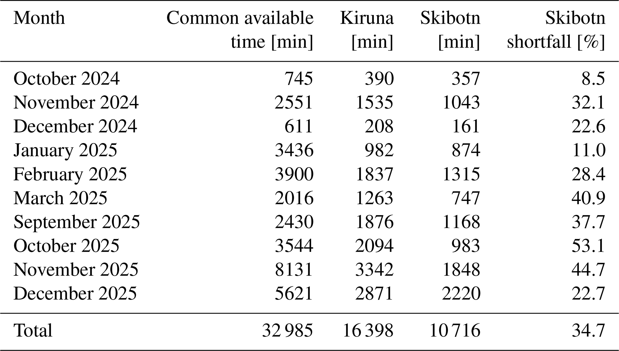
Figure B1b shows the fraction of the observable exposure shown in Fig. B1a that was classified as PsA. To exclude statistically unstable bins, Fig. B1b and c display only MLT/MLAT bins with at least 5 h of observable exposure. When the numerators and denominators of the bins satisfying this criterion are summed separately for each site, the fraction of observable time occupied by PsA is 42.8 % at Kiruna and 24.8 % at Skibotn. At both sites, this fraction also tends to increase toward the morning sector. Therefore, the larger number of PsA keograms at Kiruna cannot be explained solely by its longer observable exposure; there is also a site-to-site difference in the fraction of observable time when PsA occurred.

Figure B1c shows the fraction of time classified as PsA when IM was identified. This fraction is 37.3 % at Kiruna and 26.6 % at Skibotn, remaining higher at Kiruna even after normalization by both observable exposure and the occurrence frequency of PsA itself. In addition, the tendency for the IM fraction to increase toward the morning sector is evident at both sites. On the other hand, the site-to-site difference decreases from 17.9 % in the PsA fraction relative to observable time to 10.7 % in the IM fraction relative to PsA time. This indicates that part of the difference in the number of keograms and in the total duration of observed IM arises from differences in observational opportunity and in the occurrence frequency of PsA itself, while a difference in the IM fraction remains even after these effects are taken into account.