Ion beam instability model for Mercury's upstream waves

An analytical model for ion beam instability is constructed in view of application to Mercury's upstream waves. Our ion beam instability model determines the frequency and wavenumber by equating the whistler dispersion relation to the beam resonance condition for planetary foreshock wave excitation. By introducing a Doppler shift into the instability frequency, our model can derive the observer-frame relation of the resonance frequency to the beam velocity and the flow speed. The frequency relation will serve as a useful diagnostic tool for Mercury upstream wave studies in the upcoming BepiColombo observations.

1 Introduction

The upstream region of the Mercury bow shock is unique in the plasma physical sense in that the low-frequency electromagnetic waves are excited in the nearly radial interplanetary direction to the Sun and in a moderate Mach number flow below 10. Diffuse and field-aligned beam and low-frequency waves are detected by the MESSENGER spacecraft (e.g., Le et al., 2013; Romanelli and DiBraccio, 2021; Glass et al., 2023), the mechanism of which is reminiscent of the Earth foreshock formation. Naive calculation gives a Parker spiral angle of about 20° to the radial direction of the Sun. The MESSENGER magnetic field and the ENLIL (Odstrcil, 2003; Odstrcil et al., 2004, 2005) model calculation estimate that the flow speed is about 350–400 km s⁻¹, which corresponds to an Alfvén–Mach number of around 6.

Various kinds of low-frequency electromagnetic waves are observed upstream of the Mercury bow shock by the MESSENGER spacecraft, e.g., the whistler-mode wave at about 2 Hz (in the spacecraft frame), the fast-mode wave at about 0.3 Hz (Le et al., 2013), and the ion cyclotron associated with the pickup protons (Schmid et al., 2022). Here we propose that the right-hand-side resonant instability driven by the beam ions can explain both the whistler and magnetosonic modes below or around the ion cyclotron frequency (for protons) such as the waves at 0.3 Hz in the spacecraft frame (the proton cyclotron frequency is about 0.46 Hz for a magnetic field magnitude of 30 nT) and the pickup ion cyclotron waves. The wave excitation at a higher frequency such as 2 Hz in the spacecraft frame needs a modification of our model, such as an antisunward-streaming ion beam in the observer frame, parametric instabilities, or a sunward-streaming electron beam. The lesson from the Earth foreshock studies is that the foreshock waves are driven by the shock-reflected back-streaming ions interacting with the solar wind, and the waves are driven by the right-hand-side resonant ion beam instability, also referred to as the component–component instability (Gary, 1993). The pickup ion cyclotron waves are unique to the extended exospheric region in that the neutral species (atomic hydrogen) is photo-ionized in interplanetary space and is observed around Mercury (Schmid et al., 2022) as well as Venus and Mars (Delva et al., 2011a, b).

Both the foreshock and ion cyclotron waves exhibit left-hand-side field rotation about the mean magnetic field in the temporal sense when seen in the spacecraft frame, because the right-hand-side beam resonance undergoes a Doppler shift in the direction opposite to the beam and the wave polarization is reversed in a left-hand-side rotation sense. The pickup ion cyclotron waves are also observed in a left-hand-side field rotation sense because the spacecraft frame is virtually the same as the rest frame of the pickup ions.

We develop an analytical model of the ion beam instability that is relevant to Mercury's upstream waves in view of the upcoming arrival of the BepiColombo mission at Mercury (Benkhoff et al., 2021). Our foreshock model is constructed of the dispersion relation of whistler waves and the beam resonance condition. We derive a constraint relation between the frequency (or wavenumber) of the instability, the beam velocity, and the flow speed. The model has the capability to estimate the flow speed if the beam velocity is known or assumed or vice versa to estimate the beam velocity if the flow speed is known or assumed. In particular, the Mio spacecraft of BepiColombo covers a wide range of radial distances to Mercury of up to about 6 planetary radii, which is suitable for performing a systematic survey of Mercury's upstream waves with a magnetometer and plasma detectors. Our model serves as a diagnostic tool for determining or constraining the velocities (flow speed and beam velocity) when using the magnetic field data.

2 Resonance frequency estimate

2.1 Problem setup

In the theoretical framework, the beam instability is conveniently analyzed in the rest frame of the bulk plasma. We refer to this as the flow frame, co-moving with the solar wind. The ion beam is injected into the system at a speed of U_b (the beam direction is taken to be positive) along the magnetic field. See Fig. 1a for the flow frame setup. In order to interpret the beam instability in the observer frame (representative of the spacecraft frame), the Galilean transformation is introduced with a flow speed U_f (taken to be negative in the direction opposite to the beam). The beam velocity reduces to U_f+U_b (see Fig. 1b). The observer frame may also be regarded as the shock frame such that the beam velocity is U_f+U_b with respect to the bow shock.

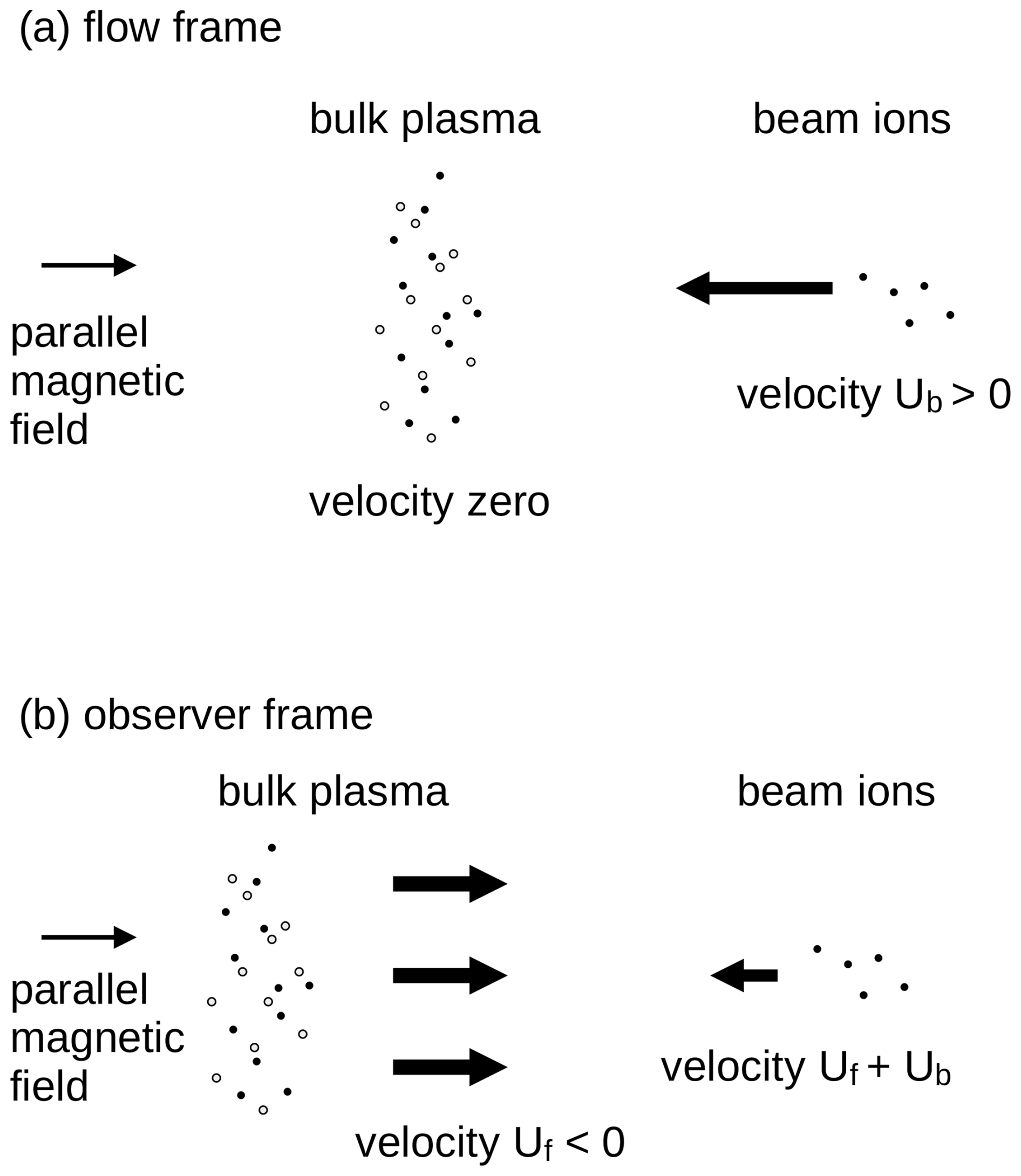
Figure 1 Ion beam injected into the bulk plasma in the flow frame (a) and in the observer frame (b).

2.2 Analysis in the flow frame

The right-hand-side resonant instability represents an energy and momentum transfer of the beam ions into the electromagnetic waves. The kinetic treatment of the beam instabilities is documented in the framework of linear Vlasov theory by Gary (1993). Single-spacecraft and multi-spacecraft observations in the Earth foreshock region confirm the right-hand-side resonant instability (Watanabe and Terasawa, 1984; Eastwood et al., 2003; Narita et al., 2003).

The right-hand-side resonant instability occurs when the low-frequency whistler mode (R⁺ branch) meets the beam resonance condition. The resonance occurs at a frequency below or around the ion cyclotron frequency. Figure 2 illustrates the dispersion relation diagram of four branches of electromagnetic waves, with R⁺ the right-hand-side polarized parallel-propagating mode (whistler mode with positive helicity), R⁻ the left-hand-side polarized antiparallel-propagating mode (ion cyclotron mode with positive helicity), L⁺ the left-hand-side polarized parallel-propagating mode (ion cyclotron mode with negative helicity), and L⁻ the right-hand-side polarized antiparallel-propagating mode (whistler mode with negative helicity). The symbols R and L represent the dielectric response or the wave helicity (spatial field rotation sense around the mean magnetic field), and the plus and minus signs represent the propagation direction with respect to the mean magnetic field.

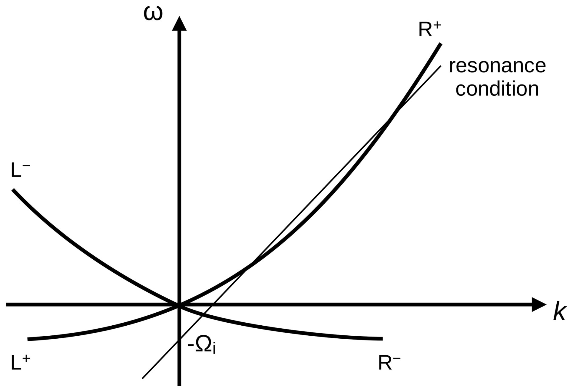
Figure 2 Dispersion relations and the beam resonance condition. Protons are assumed for the bulk ions and beam ions with the cyclotron frequency Ω_i. The wave modes are the whistler wave propagating forward (R⁺ mode) and backward (L⁻ mode) to the mean magnetic field and the ion cyclotron wave propagating forward (L⁺ mode) and backward (R⁻ mode). The symbols R and L refer to the polarization, i.e., the dielectric response in the STIX notation, and the plus and minus signs refer to the propagation sense with respect to the mean magnetic field. The beam resonance condition is indicated by the thin line and intersects the y axis (long-wavelength limit), with the ion cyclotron frequency in the negative frequency domain. The beam resonance with the R⁺ mode is considered here. Resonance with the R⁻ mode is unlikely because of the opposite group velocity direction to the beam (no sufficient time for the energy exchange).

The task is to find the crossing frequency between the R⁺ branch and the resonance condition. The low-frequency part of the whistler dispersion relation for parallel propagation in a low-beta plasma (cold plasma), by including the effect of the Hall current, is obtained after Hasegawa and Uberoi (Eq. 2.24 in 1982) or Gary (Eq. 6.2.5 in 1993) as

$$\begin{array}{}\text{(1)}& {\displaystyle \frac{\mathit{\omega }}{{\mathrm{\Omega }}_{\mathrm{i}}}}& {\displaystyle }\simeq {\displaystyle \frac{k_{\Vert }{V}_{\mathrm{A}}}{{\mathrm{\Omega }}_{\mathrm{i}}}}{\left(\mathrm{1}+{\displaystyle \frac{k_{\Vert }{V}_{\mathrm{A}}}{{\mathrm{\Omega }}_{\mathrm{i}}}}\right)}^{\mathrm{1}/\mathrm{2}}\text{(2)}& {\displaystyle }& {\displaystyle }\simeq {\displaystyle \frac{k_{\Vert }{V}_{\mathrm{A}}}{{\mathrm{\Omega }}_{\mathrm{i}}}}+{\displaystyle \frac{\mathrm{1}}{\mathrm{2}}}{\left({\displaystyle \frac{k_{\Vert }{V}_{\mathrm{A}}}{{\mathrm{\Omega }}_{\mathrm{i}}}}\right)}^{\mathrm{2}}.\end{array}$$

The resonance condition for the beam ions (assumed to be protons) is expressed as

$$\begin{array}{}\text{(3)}& \mathit{\omega }-k_{\Vert }{U}_{\mathrm{b}}=-{\mathrm{\Omega }}_{\mathrm{i}}.\end{array}$$

Here, ω denotes the wave frequency, k the wavenumber parallel to the mean magnetic field, V_A the Alfvén speed, and Ω_i the ion cyclotron frequency for protons.

For an easier theoretical treatment, we normalize the frequency to the ion cyclotron frequency (for the protons) Ω_i and rewrite hereafter the normalized frequency as $\stackrel{\mathrm{̃}}{\mathit{\omega }}=\mathit{\omega }/{\mathrm{\Omega }}_{\mathrm{i}}$. The proton cyclotron frequency is then expressed as unity, i.e., ${\stackrel{\mathrm{̃}}{\mathrm{\Omega }}}_{\mathrm{i}}=\mathrm{1}$. The wavenumber is accordingly normalized to the ion inertial length $V_{\mathrm{A}}/{\mathrm{\Omega }}_{\mathrm{i}}$, and we rewrite the normalized wavenumber as $\stackrel{\mathrm{̃}}{k}=k{V}_{\mathrm{A}}/{\mathrm{\Omega }}_{\mathrm{i}}$. The same normalization applies to the parallel wavenumber. When limited to the parallel propagation, the whistler dispersion relation (Eq. 1) and the resonance condition are rewritten as

$$\begin{array}{}\text{(4)}& \stackrel{\mathrm{̃}}{\mathit{\omega }}={\stackrel{\mathrm{̃}}{k}}_{\Vert }+{\displaystyle \frac{\mathrm{1}}{\mathrm{2}}}{\stackrel{\mathrm{̃}}{k}}_{\Vert }^{\mathrm{2}}\end{array}$$

and

$$\begin{array}{}\text{(5)}& \stackrel{\mathrm{̃}}{\mathit{\omega }}-{\stackrel{\mathrm{̃}}{k}}_{\Vert }{\stackrel{\mathrm{̃}}{U}}_{\mathrm{b}}=-\mathrm{1}.\end{array}$$

The beam velocity is normalized to the Alfvén speed as ${\stackrel{\mathrm{̃}}{U}}_{\mathrm{b}}=U_{\mathrm{b}}/V_{\mathrm{A}}$.

By eliminating the frequency ω in Eqs. (4) and (5), we obtain the quadratic equation for the resonance wavenumber:

$$\begin{array}{}\text{(6)}& {\stackrel{\mathrm{̃}}{k}}_{\Vert }^{\mathrm{2}}-\mathrm{2}({\stackrel{\mathrm{̃}}{U}}_{\mathrm{b}}-\mathrm{1}){\stackrel{\mathrm{̃}}{k}}_{\Vert }+\mathrm{2}=\mathrm{0}.\end{array}$$

The roots of Eq. (6) are

$$\begin{array}{}\text{(7)}& {\displaystyle }{\stackrel{\mathrm{̃}}{k}}_{\Vert }={\stackrel{\mathrm{̃}}{U}}_{\mathrm{b}}-\mathrm{1}\pm \sqrt{({\stackrel{\mathrm{̃}}{U}}_{\mathrm{b}}-{\stackrel{\mathrm{̃}}{U}}_{-})({\stackrel{\mathrm{̃}}{U}}_{\mathrm{b}}-{\stackrel{\mathrm{̃}}{U}}_{+})},\text{(8)}& {\displaystyle }{\stackrel{\mathrm{̃}}{U}}_{\pm }=\mathrm{1}\pm \sqrt{\mathrm{2}}.\end{array}$$

For the existence of a real-number solution, the beam velocity must satisfy the condition

$$\begin{array}{}\text{(9)}& {\stackrel{\mathrm{̃}}{U}}_{\mathrm{b}}\ge {\stackrel{\mathrm{̃}}{U}}_{+}=\mathrm{1}+\sqrt{\mathrm{2}}.\end{array}$$

Interestingly, the threshold value is about $\mathrm{1}+\sqrt{\mathrm{2}}\sim \mathrm{2.4}$, which is close to the critical Alfvén–Mach number for the shock reflection mechanism. The wave–particle interaction is considered to sufficiently scatter the particles in a low Mach number shock up to an Alfvén–Mach number of about 2.7 (subcritical shocks). In a high Mach number shock (Alfvén–Mach number above 2.7), the dissipation is primarily created by the specular reflection of the cross-shock potential and the wave–particle interactions at the shock transition. Our theory predicts that the critical-beam Mach number will be about 2.4. There might be a relation between the dissipation mechanism and the ion beam instability in the collisionless shock such that the beam instability will potentially contribute to a more efficient shock dissipation.

The lower wavenumber solution of Eq. (7) with the minus sign is the resonance wavenumber of interest. The higher wavenumber solution is valid for a lower beam velocity near the “touch point” (Eq. 9) but may not be exact for a higher beam velocity as the parabolic approximation of the whistler mode is no longer valid at higher frequencies. The resonance frequency in the flow frame is derived from Eq. (5) as

$$\begin{array}{}\text{(10)}& \mathit{\omega }=\left({\stackrel{\mathrm{̃}}{U}}_{\mathrm{b}}-\mathrm{1}-\sqrt{({\stackrel{\mathrm{̃}}{U}}_{\mathrm{b}}-{\stackrel{\mathrm{̃}}{U}}_{-})({\stackrel{\mathrm{̃}}{U}}_{\mathrm{b}}-{\stackrel{\mathrm{̃}}{U}}_{+})}\right){\stackrel{\mathrm{̃}}{U}}_{\mathrm{b}}-\mathrm{1}.\end{array}$$

2.3 Transformation into the observer frame

By introducing the Doppler shift through the bulk flow as ${\stackrel{\mathrm{̃}}{k}}_{\Vert }{\stackrel{\mathrm{̃}}{U}}_{\mathrm{f}}$ (here ${\stackrel{\mathrm{̃}}{U}}_{\mathrm{f}}$ denotes the flow speed in the units of the Alfvén speed) in the direction opposite to the beam velocity and transforming the frequency from the flow rest frame into the observer frame, we obtain the resonance frequency ${\stackrel{\mathrm{̃}}{\mathit{\omega }}}^{\prime }$ (in the units of the proton cyclotron frequency) as

$$\begin{array}{}\text{(11)}& {\displaystyle }{\stackrel{\mathrm{̃}}{\mathit{\omega }}}^{\prime }& {\displaystyle }={\stackrel{\mathrm{̃}}{k}}_{\Vert }({\stackrel{\mathrm{̃}}{U}}_{\mathrm{b}}+{\stackrel{\mathrm{̃}}{U}}_{\mathrm{f}})-\mathrm{1}\text{(12)}& {\displaystyle }& {\displaystyle }=\left[({\stackrel{\mathrm{̃}}{U}}_{\mathrm{b}}-\mathrm{1})-\sqrt{({\stackrel{\mathrm{̃}}{U}}_{\mathrm{b}}-{\stackrel{\mathrm{̃}}{U}}_{-})({\stackrel{\mathrm{̃}}{U}}_{\mathrm{b}}-{\stackrel{\mathrm{̃}}{U}}_{+})}\right]\times ({\stackrel{\mathrm{̃}}{U}}_{\mathrm{b}}+{\stackrel{\mathrm{̃}}{U}}_{\mathrm{f}})-\mathrm{1}.\end{array}$$

Figure 3a displays the dispersion relation and the resonance condition in the co-moving frame and the observer frame for the foreshock ions with a beam velocity of ${\stackrel{\mathrm{̃}}{U}}_{\mathrm{b}}=\mathrm{7}$ and a flow speed of ${\stackrel{\mathrm{̃}}{U}}_{\mathrm{f}}=-\mathrm{5}$. Whistler wave frequencies are transformed into the negative frequency domain while retaining the wavenumber. The temporal sense of wave field rotation (polarization) changes accordingly from right-hand-side rotation around the magnetic field to left-hand-side rotation.

Figure 3b displays the dispersion relation and resonance condition for a beam velocity canceling the flow speed ${\stackrel{\mathrm{̃}}{U}}_{\mathrm{b}}=-{\stackrel{\mathrm{̃}}{U}}_{\mathrm{f}}=\mathrm{5}$ for the pickup ion scenario. The resonance frequency is the ion cyclotron frequency with the left-hand-side sense of field rotation in the observer frame.

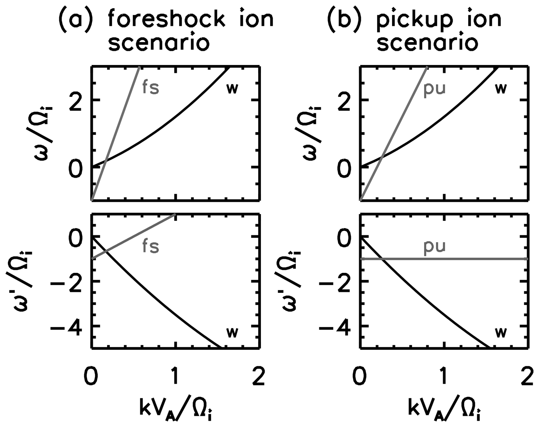
Figure 3 Whistler dispersion relation (in black) and beam resonance condition (in gray) in the co-moving frame with the flow (top panels) and the observer frame standing in the flow (bottom panels). A beam velocity of $U_{\mathrm{b}}/V_{\mathrm{A}}=\mathrm{7}$ and a flow speed of $U_{\mathrm{f}}/V_{\mathrm{A}}=-\mathrm{5}$ are chosen for the foreshock ion scenario (a). The beam velocity canceling the flow speed is chosen for the pickup ion scenario (b) $U_{\mathrm{b}}/V_{\mathrm{A}}=-U_{\mathrm{f}}/V_{\mathrm{A}}=\mathrm{5}$.

Equation (12) relates the resonance frequency (e.g., the peak of the magnetic power spectrum in the spacecraft frame) to the beam velocity and the flow speed. The frequency estimate (Eq. 12) indicates that the ion cyclotron frequency is expected for the beam instability for the pickup ions by substituting the sign-reversed flow speed into the beam velocity as ${\stackrel{\mathrm{̃}}{U}}_{\mathrm{b}}=-{\stackrel{\mathrm{̃}}{U}}_{\mathrm{f}}$ (pickup ion cyclotron waves).

3 Velocity estimate

Equation (12) may be regarded as a function of the beam velocity in the flow frame ${\stackrel{\mathrm{̃}}{U}}_{\mathrm{b}}$ and the flow speed ${\stackrel{\mathrm{̃}}{U}}_{\mathrm{f}}$ given that the frequency is known in the observer frame. A useful tool can be developed from Eq. (12). That is, we derive the relation between the beam velocity in the observer frame ${\stackrel{\mathrm{̃}}{U}}_{\mathrm{b}}^{\prime }$ defined as

$$\begin{array}{}\text{(13)}& {\stackrel{\mathrm{̃}}{U}}_{\mathrm{b}}^{\prime }={\stackrel{\mathrm{̃}}{U}}_{\mathrm{b}}+{\stackrel{\mathrm{̃}}{U}}_{\mathrm{f}}\end{array}$$

and the flow speed ${\stackrel{\mathrm{̃}}{U}}_{\mathrm{f}}$ for the resonance frequency ${\stackrel{\mathrm{̃}}{\mathit{\omega }}}^{\prime }$. We can derive the expression of ${\stackrel{\mathrm{̃}}{U}}_{\mathrm{b}}$ by transforming Eq. (12) into

$$\begin{array}{}\text{(14)}& {\displaystyle \frac{{\stackrel{\mathrm{̃}}{\mathit{\omega }}}^{\prime }+\mathrm{1}}{{\stackrel{\mathrm{̃}}{U}}_{\mathrm{b}}^{\prime }}}-({\stackrel{\mathrm{̃}}{U}}_{\mathrm{b}}-\mathrm{1})=-\sqrt{({\stackrel{\mathrm{̃}}{U}}_{\mathrm{b}}-{\stackrel{\mathrm{̃}}{U}}_{-})({\stackrel{\mathrm{̃}}{U}}_{\mathrm{b}}-{\stackrel{\mathrm{̃}}{U}}_{+})}\end{array}$$

and squaring Eq. (14) as

$$\begin{array}{}\text{(15)}& {\left[{\displaystyle \frac{{\stackrel{\mathrm{̃}}{\mathit{\omega }}}^{\prime }+\mathrm{1}}{{\stackrel{\mathrm{̃}}{U}}_{\mathrm{b}}^{\prime }}}-({\stackrel{\mathrm{̃}}{U}}_{\mathrm{b}}-\mathrm{1})\right]}^{\mathrm{2}}={\stackrel{\mathrm{̃}}{(U}}_{\mathrm{b}}-{\stackrel{\mathrm{̃}}{U}}_{-}\left)\right({\stackrel{\mathrm{̃}}{U}}_{\mathrm{b}}-{\stackrel{\mathrm{̃}}{U}}_{+}).\end{array}$$

Equation (15) is simplified to

$$\begin{array}{}\text{(16)}& {\stackrel{\mathrm{̃}}{U}}_{\mathrm{b}}={\displaystyle \frac{{\stackrel{\mathrm{̃}}{\mathit{\omega }}}^{\prime }+\mathrm{1}}{\mathrm{2}{\stackrel{\mathrm{̃}}{U}}_{\mathrm{b}}^{\prime }}}+{\displaystyle \frac{{\stackrel{\mathrm{̃}}{U}}_{\mathrm{b}}^{\prime }}{{\stackrel{\mathrm{̃}}{\mathit{\omega }}}^{\prime }+\mathrm{1}}}+\mathrm{1}.\end{array}$$

We combine Eq. (16) with Eq. (13) and obtain ${\stackrel{\mathrm{̃}}{U}}_{\mathrm{f}}$ as a function of ${\stackrel{\mathrm{̃}}{U}}_{\mathrm{b}}^{\prime }$ as

$$\begin{array}{}\text{(17)}& {\stackrel{\mathrm{̃}}{U}}_{\mathrm{f}}=-{\displaystyle \frac{{\stackrel{\mathrm{̃}}{\mathit{\omega }}}^{\prime }+\mathrm{1}}{\mathrm{2}{\stackrel{\mathrm{̃}}{U}}_{\mathrm{b}}^{\prime }}}+\left(\mathrm{1}-{\displaystyle \frac{\mathrm{1}}{{\stackrel{\mathrm{̃}}{\mathit{\omega }}}^{\prime }+\mathrm{1}}}\right){\stackrel{\mathrm{̃}}{U}}_{\mathrm{b}}^{\prime }-\mathrm{1}.\end{array}$$

Figure 4 is the graphical representation of Eq. (17) at various values of ${\stackrel{\mathrm{̃}}{\mathit{\omega }}}^{\prime }$. Three conditions are imposed for ${\stackrel{\mathrm{̃}}{U}}_{\mathrm{f}}$ and ${\stackrel{\mathrm{̃}}{U}}_{\mathrm{b}}^{\prime }$. First, the flow must be in the negative direction (opposite to the beam) in the observer frame, i.e., ${\stackrel{\mathrm{̃}}{U}}_{\mathrm{f}}<\mathrm{0}$. Second, the beam velocity must be in the positive direction in the observer frame for the formation of the foreshock region, i.e., ${\stackrel{\mathrm{̃}}{U}}_{\mathrm{b}}^{\prime }>\mathrm{0}$. Third, the beam resonance must occur, so ${\stackrel{\mathrm{̃}}{U}}_{\mathrm{b}}>{\stackrel{\mathrm{̃}}{U}}_{+}$ in the flow frame (Eq. 9), which is transformed into ${\stackrel{\mathrm{̃}}{U}}_{\mathrm{f}}<{\stackrel{\mathrm{̃}}{U}}_{\mathrm{b}}^{\prime }-U_{+}$ in the observer frame. The velocity diagram shows the relation between the flow speed and the beam velocity if the resonance frequency is set or known. The flow speed has a positive slope to smaller values of the beam velocity (typically ${\stackrel{\mathrm{̃}}{U}}_{\mathrm{b}}^{\prime }\lesssim \mathrm{0.5}$), while the slope becomes negative at larger values of the beam velocity (${\stackrel{\mathrm{̃}}{U}}_{\mathrm{b}}^{\prime }\gtrsim \mathrm{0.5}$).

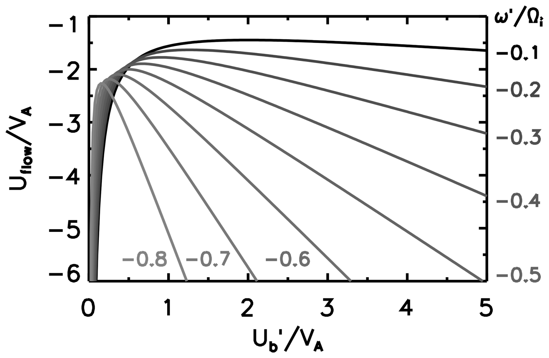
Figure 4 Velocity diagram showing the flow speed (normalized to the Alfvén speed) $U_{\mathrm{f}}/V_{\mathrm{A}}$ as a function of the beam velocity (also normalized to the Alfvén speed) in the observer frame ${\stackrel{\mathrm{̃}}{U}}_{\mathrm{b}}^{\prime }/V_{\mathrm{A}}$ at different values of the resonance frequency (normalized to the proton cyclotron frequency) in the observer frame ${\stackrel{\mathrm{̃}}{\mathit{\omega }}}^{\prime }/{\mathrm{\Omega }}_{\mathrm{i}}$.

One can develop a useful tool from Eq. (17) and knowledge from Earth foreshock studies, since the beam velocity is nearly the same as the Alfvén speed in the flow rest frame (Narita et al., 2003). We determine the flow speed as a function of the observer-frame frequency at several representative values of beam velocity (in the observer frame) and plot the diagram in Fig. 5. For the beam velocity on the order of Alfvén speed or higher, $U_{\mathrm{b}}^{\prime }\gtrsim V_{\mathrm{A}}$, which is the estimated flow speed, is a monotonous function of the observer-frame frequency. The flow velocity increases more rapidly at higher frequencies (typically ${\mathit{\omega }}^{\prime }/{\mathrm{\Omega }}_{\mathrm{i}}\gtrsim \mathrm{0.4}$). Figure 5 gives us a range of the estimated flow speed if the range of the beam velocity is set.

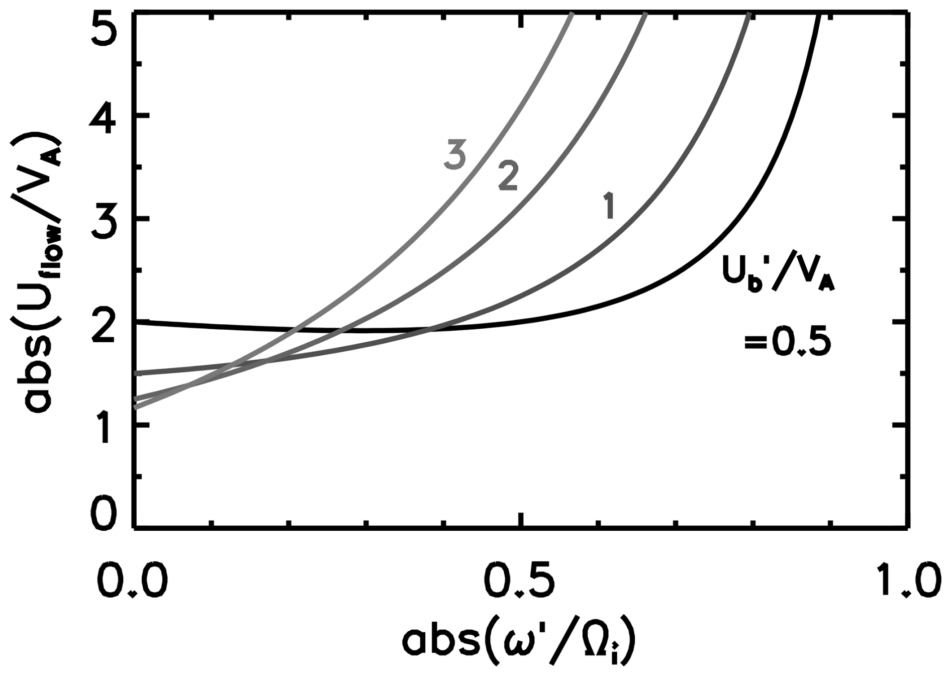
Figure 5 Flow speed diagram as a function of the resonance frequency in the observer frame at different beam velocities. Absolute values of the frequency and flow speed are used in the plot.

4 Discussion

4.1 Validity of the model

We constructed our beam instability model under non-relativistic, low-frequency, and low-beam-density conditions. We discuss the validity of the model as follows:

1. Galilean approximation.

   The solar wind speed is about 400 km s⁻¹ at the distance of Mercury's orbit (0.3 to 0.4 astronomical units). The back-streaming ion beam velocity is in the range from 500 to 1000 km s⁻¹ (e.g., Glass et al., 2023). In total, the velocity of up to 1500 km s⁻¹ is in the likely range of the velocities considered in our model. The ratio of the velocity to the speed of light (Lorentz factor beta) is estimated as β=0.005, and the Lorentz factor gamma is γ=1.0000125. The Galilean approximation is sufficient in our model. See Appendix B for the relativistic treatment.

2. Low-frequency approximation.

   Our model breaks down at shorter wavelengths (higher wavenumbers) because the second-order Taylor expansion (parabolic fitting) of the whistler dispersion relation is no longer valid at shorter wavelengths. Our model is valid at a wavelength (of the low-frequency whistler mode) from MHD scales (typically about 1000 km and above in the solar wind) down to about the ion inertial length (down to about 100 km).

3. Low beam density.

   Our model is valid for a low density of beam ions (typically below 0.1 % of the bulk ion density). When the beam density is higher, the resonance condition changes in two ways. First, the beam resonance occurs in a wider range of wavenumbers (the growth rate has a finite width in the wavenumber domain) around the resonance wavenumber (the minus-sign version of Eq. 8). Second, the fire-hose instability is set by the beam contributing to the dynamic pressure parallel to the mean magnetic field. The beam–fire-hose instability occurs in the MHD regime such that the R and L modes are not yet dispersive in the long-wavelength limit.

4.2 Deviation from parallel propagation

Smaller angular misalignment of the wave propagation direction from the mean magnetic field has no significant impact on the resonance condition. Qualitatively speaking, obliquely propagating whistler-mode waves are elliptically polarized and thus have both right-hand-side and left-hand-side polarized components. The elliptic polarization implies the possibility of beam resonance, not only with the right-hand-side component, but also with the left-hand-side component. The transition into the left-hand-side beam resonance occurs, however, at a larger propagation angle of 45–60° to the mean magnetic field (Verscharen and Chandran, 2013; Narita and Motschmann, 2025).

Figure 6 displays the dispersion relations and the growth rate for parallel propagation angles of θ_kB=0, 10, and 20°. The unstable mode has no practical difference in the wavenumber domain ($\mathrm{0.25}\le kc/{\mathit{\omega }}_{\mathrm{pi}}\le \mathrm{0.28}$) between the case of θ_kB=0° and that of θ_kB=10°. The wavenumber range of the unstable mode becomes slightly higher at θ_kB=20° ($\mathrm{0.26}\le kc/{\mathit{\omega }}_{\mathrm{pi}}\le \mathrm{0.29}$).

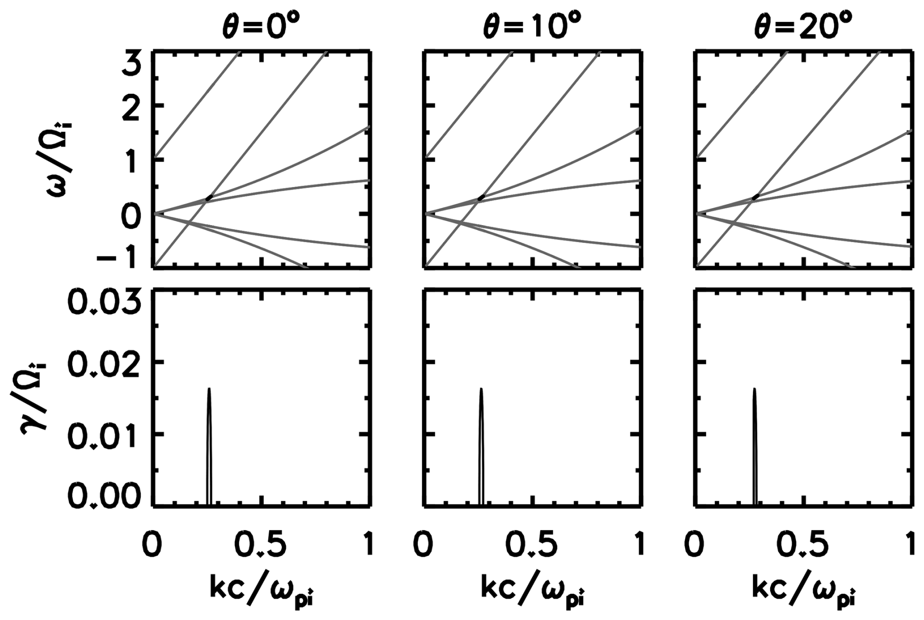
Figure 6 Linear instability analysis using the cold plasma dielectric tensor for wave propagation angles of 0, 10, and 20° to the mean magnetic field.

4.3 Magnetic field oblique to the bulk flow

The model can be upgraded to a mean magnetic field oblique to the bulk flow direction by projecting the flow velocity onto the mean magnetic field. The Doppler shift term changes from ${\stackrel{\mathrm{̃}}{k}}_{\Vert }{\stackrel{\mathrm{̃}}{U}}_{\mathrm{f}}$ to ${\stackrel{\mathrm{̃}}{k}}_{\Vert }{\stackrel{\mathrm{̃}}{U}}_{\mathrm{f}}\cos \mathit{\theta }$, where θ is the angle between the flow direction and the axis of the mean magnetic field. A smaller value of the angle is used from the mean field direction or the direction opposite to the mean field such that the projection does not change sign ($\mathrm{0}\le \cos \mathit{\theta }\le \mathrm{1}$).

4.4 Heavier ion species

The Mercury plasma environment has heavier ions other than protons. Examples are helium alpha particles (${\mathrm{He}}^{++}$) of solar wind origin and molecular or atomic species of exospheric origin such as ${\mathrm{H}}_{\mathrm{2}}^{+}$, Li⁺, and Na⁺.

• The helium alpha particles stream in the antisunward direction. The alpha particles may have a different flow speed from the bulk flow speed of the solar wind (electron–proton plasma) and can potentially drive the beam instability by resonating with the whistler or ion cyclotron mode (e.g., Verscharen and Chandran, 2013), but this instability scenario is intrinsic to the solar wind. Specular reflection of the helium alpha particles at the shock is unlikely because the protons are most easily accelerated by the electrostatic shock potential back to the solar wind to form the foreshock region. The back-streaming alpha particles have so far not been reported in the shock upstream region.

• Exospheric particles may be present in the shock upstream region. The beam velocity is so small (the escape velocity is about 4 km s⁻¹ at Mercury) compared to the solar wind speed (about 400 km s⁻¹) that the waves driven by the beam instability appear as pickup ion cyclotron waves. In this scenario, it is impossible to estimate the flow speed because the frequency is the ion cyclotron frequency in the observer frame.

We can nevertheless generalize the instability model to the beam of heavier ion species. Equation (5) is generalized to

$$\begin{array}{}\text{(18)}& \stackrel{\mathrm{̃}}{\mathit{\omega }}-{\stackrel{\mathrm{̃}}{k}}_{\Vert }{\stackrel{\mathrm{̃}}{U}}_{\mathrm{b}}=-{\displaystyle \frac{\mathrm{1}}{n}},\end{array}$$

where we introduced the mass-per-charge factor of n. For example, the alpha particles ${\mathrm{He}}^{++}$ are characterized by the normalized cyclotron frequency $\mathrm{1}/\mathrm{2}$ (i.e., n=2), the helium singular ionized state by the frequency $\mathrm{1}/\mathrm{4}$ (n=4), and so on. A combination of Eq. (18) and Eq. (4) gives the resonance wavenumber as

$$\begin{array}{}\text{(19)}& {\stackrel{\mathrm{̃}}{k}}_{\Vert }={\stackrel{\mathrm{̃}}{U}}_{\mathrm{b}}-\mathrm{1}-\sqrt{({\stackrel{\mathrm{̃}}{U}}_{\mathrm{b}}-\mathrm{1}{)}^{\mathrm{2}}-{\displaystyle \frac{\mathrm{2}}{n}}}\end{array}$$

and the resonance frequency in the observer frame as

$$\begin{array}{}\text{(20)}& {\stackrel{\mathrm{̃}}{\mathit{\omega }}}^{\prime }=\left[{\stackrel{\mathrm{̃}}{U}}_{\mathrm{b}}-\mathrm{1}-\sqrt{({\stackrel{\mathrm{̃}}{U}}_{\mathrm{b}}-\mathrm{1}{)}^{\mathrm{2}}-{\displaystyle \frac{\mathrm{2}}{n}}}\right]({\stackrel{\mathrm{̃}}{U}}_{\mathrm{b}}+{\stackrel{\mathrm{̃}}{U}}_{\mathrm{f}})-{\displaystyle \frac{\mathrm{1}}{n}}.\end{array}$$

The resonance wavenumber and the resonance frequency approach zero (${\stackrel{\mathrm{̃}}{k}}_{\Vert }\to \mathrm{0}$ and ${\stackrel{\mathrm{̃}}{\mathit{\omega }}}^{\prime }\to \mathrm{0}$) for a larger value of the mass-per-charge factor n→∞. For the pickup ions, the beam velocity is the flow velocity with the opposite sign, and ${\stackrel{\mathrm{̃}}{U}}_{\mathrm{b}}+{\stackrel{\mathrm{̃}}{U}}_{\mathrm{f}}=\mathrm{0}$ holds. The resonance frequency in the observer frame is then ${\stackrel{\mathrm{̃}}{\mathit{\omega }}}^{\prime }=-\mathrm{1}/n$.

5 Concluding remarks

Our ion beam instability model determines the resonance frequency and wavenumber by equating the low-frequency whistler dispersion relation to the beam resonance condition for planetary foreshock wave excitation. The resonance is of the right-hand-side type for the R⁺ mode (whistler branch) and occurs at a beam velocity of at least ${\stackrel{\mathrm{̃}}{U}}_{\mathrm{b}}=\mathrm{1}+\sqrt{\mathrm{2}}\sim \mathrm{2.4}$ in the flow rest frame. The instability condition is likely satisfied in the near-Mercury solar wind as the Mach number is mostly above 4 after the MESSENGER observation and the ENLIL calculation (Winslow et al., 2013). It is interesting to note that the critical beam velocity ${\stackrel{\mathrm{̃}}{U}}_{\mathrm{b}}\sim \mathrm{2.4}$ roughly coincides with the critical Alfvén–Mach number for the specular reflection at the collisionless shocks (which is about 2.7).

Our model is capable of predicting the wavelength and frequency of the beam instability for the given set of beam velocity and flow speed. Here is an example. For a beam velocity of ${\stackrel{\mathrm{̃}}{U}}_{\mathrm{b}}^{\prime }=\mathrm{1}$ in the observer frame and a flow Mach number of 6 in the direction opposite to the beam ${\stackrel{\mathrm{̃}}{U}}_{\mathrm{f}}=-\mathrm{6}$ (e.g., Winslow et al., 2013), we obtain the beam velocity in the flow frame as ${\stackrel{\mathrm{̃}}{U}}_{\mathrm{b}}={\stackrel{\mathrm{̃}}{U}}_{\mathrm{b}}+{\stackrel{\mathrm{̃}}{U}}_{\mathrm{f}}=\mathrm{7}$. The resonance wavenumber is estimated as $k_{\Vert }{V}_{\mathrm{A}}/{\mathrm{\Omega }}_{\mathrm{i}}\simeq \mathrm{0.17}$ (Eq. 7) and the frequency as ${\mathit{\omega }}^{\prime }/{\mathrm{\Omega }}_{\mathrm{i}}\simeq -\mathrm{0.83}$ (Eq. 11). By referring to the magnetic field statistics of about 20 nT (Romanelli and DiBraccio, 2021) and the ion density of about 40 cm⁻³ (Winslow et al., 2013), we obtain an Alfvén speed of V_A≃70 km s⁻¹ and an ion inertial length of $V_{\mathrm{A}}/{\mathrm{\Omega }}_{\mathrm{i}}\simeq \mathrm{3.7}$ km rad⁻¹. The resonance wavelength is thus estimated as 3.5 km and the frequency as 2.5 s⁻¹, which are well within the sampling rate of the fluxgate magnetometer on board the BepiColombo Mio spacecraft, with 128 Hz for the burst mode or H mode and 8 Hz for the normal mode or M1 mode (Baumjohann et al., 2020). The back-streaming ions are observed by MESSENGER (e.g., Glass et al., 2023). The pickup ion cyclotron waves are also observed by MESSENGER (e.g., Schmid et al., 2022). A combination of the Mio MGF and Mio MPPE/MIA instruments is ideally suited to testing our instability model against the spacecraft data.

Our model is developed for a one-dimensional setup; i.e., the beam velocity, the flow, and the wave propagation are assumed to all be aligned with the mean magnetic field. Even though such an aligned situation is most likely realized in the Mercury upstream region as the Parker spiral angle here is the smallest (most radial) of all of the solar system's planets, our model may be upgraded to a weakly misaligned wave system (like the effect of inclination of the mean magnetic field to the flow direction or a moderately oblique propagation angle to the mean magnetic field) by projecting the misaligned system onto our one-dimensional treatment.

Appendix A: Dispersion relation

The dispersion relation for low-frequency, parallel-propagating whistler waves in an electron–ion plasma is shown in various forms in the literature, such as Eq. (6.2.5) in Gary (1993) and Eq. (2.24) in Hasegawa and Uberoi (1982). We start with the general form of the R-mode dispersion relation for the two-component cold plasma (electrons and ions), i.e.,

$$\begin{array}{}\text{(A1)}& {\mathit{\omega }}^{\mathrm{2}}-k^{\mathrm{2}}{c}^{\mathrm{2}}-{\displaystyle \frac{\mathit{\omega }{\mathit{\omega }}_{\mathrm{pe}}^{\mathrm{2}}}{\mathit{\omega }+{\mathrm{\Omega }}_{\mathrm{e}}}}-{\displaystyle \frac{\mathit{\omega }{\mathit{\omega }}_{\mathrm{pi}}^{\mathrm{2}}}{\mathit{\omega }+{\mathrm{\Omega }}_{\mathrm{i}}}}=\mathrm{0},\end{array}$$

where ω denotes the frequency, k the wavenumber (parallel to the mean magnetic field), c the speed of light, ω_pe the electron plasma frequency, ω_pi the ion plasma frequency, Ω_e the electron cyclotron frequency, and Ω_i the ion cyclotron frequency. See Eq. (6.2.4) in Gary (1993) for the derivation of Eq. (A1).

We now apply the low-frequency approximation. First, we neglect the first term, ω², on the left-hand side of Eq. (A1). Second, the denominator of the third term on the left-hand side of Eq. (A1) is simplified into Ω_e. We then obtain the dispersion relation as

$$\begin{array}{}\text{(A2)}& {\displaystyle }{k}^{\mathrm{2}}{c}^{\mathrm{2}}& {\displaystyle }=-{\displaystyle \frac{\mathit{\omega }{\mathit{\omega }}_{\mathrm{pe}}^{\mathrm{2}}}{{\mathrm{\Omega }}_{\mathrm{e}}}}-{\displaystyle \frac{\mathit{\omega }{\mathit{\omega }}_{\mathrm{pi}}^{\mathrm{2}}}{{\mathrm{\Omega }}_{\mathrm{i}}}}{\displaystyle \frac{\mathrm{1}}{\mathrm{1}+\frac{\mathit{\omega }}{{\mathrm{\Omega }}_{\mathrm{i}}}}}\text{(A3)}& {\displaystyle }& {\displaystyle }=-{\displaystyle \frac{\mathit{\omega }{\mathit{\omega }}_{\mathrm{pe}}^{\mathrm{2}}}{{\mathrm{\Omega }}_{\mathrm{e}}}}-{\displaystyle \frac{\mathit{\omega }{\mathit{\omega }}_{\mathrm{pi}}^{\mathrm{2}}}{{\mathrm{\Omega }}_{\mathrm{i}}}}\left[\mathrm{1}-{\displaystyle \frac{\mathit{\omega }}{{\mathrm{\Omega }}_{\mathrm{i}}}}+{\left({\displaystyle \frac{\mathit{\omega }}{{\mathrm{\Omega }}_{\mathrm{i}}}}\right)}^{\mathrm{2}}\right]\text{(A4)}& {\displaystyle }& {\displaystyle }=-\mathit{\omega }\left({\displaystyle \frac{{\mathit{\omega }}_{\mathrm{pe}}^{\mathrm{2}}}{{\mathrm{\Omega }}_{\mathrm{e}}}}+{\displaystyle \frac{{\mathit{\omega }}_{\mathrm{pi}}^{\mathrm{2}}}{{\mathrm{\Omega }}_{\mathrm{i}}}}\right)+{\displaystyle \frac{{\mathit{\omega }}^{\mathrm{2}}{\mathit{\omega }}_{\mathrm{pi}}^{\mathrm{2}}}{{\mathrm{\Omega }}_{\mathrm{i}}^{\mathrm{2}}}}-{\displaystyle \frac{{\mathit{\omega }}^{\mathrm{3}}{\mathit{\omega }}_{\mathrm{pi}}^{\mathrm{2}}}{{\mathrm{\Omega }}_{\mathrm{i}}^{\mathrm{3}}}}.\end{array}$$

Note that the second-order Taylor expansion is used when deriving Eq. (A3).

We introduce the charge neutrality of the plasma, which cancels the first term on the right-hand side of Eq. (A4). The charge neutrality reads in frequency form as

$$\begin{array}{}\text{(A5)}& {\displaystyle \frac{{\mathit{\omega }}_{\mathrm{pe}}^{\mathrm{2}}}{{\mathrm{\Omega }}_{\mathrm{e}}}}+{\displaystyle \frac{{\mathit{\omega }}_{\mathrm{pi}}^{\mathrm{2}}}{{\mathrm{\Omega }}_{\mathrm{i}}}}={\displaystyle \frac{q_{\mathrm{e}}{n}_{\mathrm{e}}+q_{\mathrm{i}}{n}_{\mathrm{i}}}{{\mathit{ϵ}}_{\mathrm{0}}{B}_{\mathrm{0}}}}=\mathrm{0},\end{array}$$

where q_e and q_i denote the electron and ion charges (including the sign), n_e and n_i the the number densities of electrons and ions, ϵ₀ the permittivity of the free space, and B₀ the magnetic field magnitude. We also rewrite the squared frequency ratio ${\mathit{\omega }}_{\mathrm{i}}^{\mathrm{2}}/{\mathrm{\Omega }}_{\mathrm{i}}^{\mathrm{2}}$ as

$$\begin{array}{}\text{(A6)}& {\displaystyle \frac{{\mathit{\omega }}_{\mathrm{pi}}^{\mathrm{2}}}{{\mathrm{\Omega }}_{\mathrm{i}}^{\mathrm{2}}}}={\displaystyle \frac{c^{\mathrm{2}}}{V_{\mathrm{A}}^{\mathrm{2}}}},\end{array}$$

where V_A denotes the Alfvén speed. Combining Eqs. (A4)–(A6), we obtain the dispersion relation as

$$\begin{array}{}\text{(A7)}& k^{\mathrm{2}}{c}^{\mathrm{2}}={\mathit{\omega }}^{\mathrm{2}}{\displaystyle \frac{c^{\mathrm{2}}}{V_{\mathrm{A}}^{\mathrm{2}}}}\left(\mathrm{1}-{\displaystyle \frac{\mathit{\omega }}{{\mathrm{\Omega }}_{\mathrm{i}}}}\right).\end{array}$$

When introducing the phase speed as

$$\begin{array}{}\text{(A8)}& v_{\mathrm{ph}}={\displaystyle \frac{\mathit{\omega }}{k}},\end{array}$$

the dispersion relation is formulated as

$$\begin{array}{}\text{(A9)}& v_{\mathrm{ph}}^{\mathrm{2}}={\displaystyle \frac{V_{\mathrm{A}}^{\mathrm{2}}}{\mathrm{1}-\frac{\mathit{\omega }}{{\mathrm{\Omega }}_{\mathrm{i}}}}},\end{array}$$

which is further simplified by Taylor-expanding the fraction to first order as

$$\begin{array}{}\text{(A10)}& v_{\mathrm{ph}}^{\mathrm{2}}\simeq V_{\mathrm{A}}^{\mathrm{2}}\left(\mathrm{1}+{\displaystyle \frac{\mathit{\omega }}{{\mathrm{\Omega }}_{\mathrm{i}}}}\right),\end{array}$$

which reproduces Eq. (2.24) in Hasegawa and Uberoi (1982).

Using the fact that the low-frequency whistler wave roughly satisfies the dispersion relation for the Alfvén wave,

$$\begin{array}{}\text{(A11)}& \mathit{\omega }\simeq k{V}_{\mathrm{A}},\end{array}$$

Eq. (A10) is written in the form

$$\begin{array}{}\text{(A12)}& {\displaystyle \frac{{\mathit{\omega }}^{\mathrm{2}}}{k^{\mathrm{2}}}}& {\displaystyle }=V_{\mathrm{A}}^{\mathrm{2}}\left(\mathrm{1}+{\displaystyle \frac{k{V}_{\mathrm{A}}}{{\mathrm{\Omega }}_{\mathrm{i}}}}\right)\text{(A13)}& {\displaystyle }& {\displaystyle }=V_{\mathrm{A}}^{\mathrm{2}}\left(\mathrm{1}+{\displaystyle \frac{kc}{{\mathit{\omega }}_{\mathrm{pi}}}}\right),\end{array}$$

which reproduces Eq. (6.2.5) in Gary (1993). Note that the ion inertial length is introduced in Eqs. (A12)–(A13) through Eq. (A6).

Appendix B: Relativistic beam resonance

Quantitatively speaking, the relativistic effect modifies the cyclotron frequency in the resonance condition as follows:

$$\begin{array}{}\text{(B1)}& \mathit{\omega }-k_{\Vert }{U}_{\mathrm{b}}={\displaystyle \frac{{\mathrm{\Omega }}_{\mathrm{i}}}{\mathit{\gamma }}}.\end{array}$$

Equation (B1) is obtained by re-formulating Eq. (3) into the relativistic covariant form as

$$\begin{array}{}\text{(B2)}& {\mathrm{\Lambda }}_{\mathit{\mu }}^{\mathrm{0}}{k}^{\mathit{\mu }}=k^{\prime \mathrm{0}},\end{array}$$

where the four-wave vectors k^μ (in the rest frame of the bulk plasma) and k^′ν (in the rest frame of the beam) are defined as

$$\begin{array}{}\text{(B3)}& {\displaystyle }{k}^{\mathit{\mu }}& {\displaystyle }=(\mathit{\omega }/c,k_{\Vert },\mathrm{0},\mathrm{0}),\text{(B4)}& {\displaystyle }{k}^{\prime \mathit{\nu }}& {\displaystyle }=({\mathrm{\Omega }}_{\mathrm{i}}/c,k_{\Vert }^{\prime },\mathrm{0},\mathrm{0}).\end{array}$$

The Lorentz transformation matrix ${\mathrm{\Lambda }}_{\mathit{\mu }}^{\mathit{\nu }}$ is defined as

$$\begin{array}{}\text{(B5)}& {\mathrm{\Lambda }}_{\mathit{\mu }}^{\mathit{\nu }}=\left[\begin{array}{cccc}\mathit{\gamma }& -\mathit{\gamma }\mathit{\beta }& \mathrm{0}& \mathrm{0}\\ -\mathit{\gamma }\mathit{\beta }& \mathit{\gamma }& \mathrm{0}& \mathrm{0}\\ \mathrm{0}& \mathrm{0}& \mathrm{1}& \mathrm{0}\\ \mathrm{0}& \mathrm{0}& \mathrm{0}& \mathrm{1}\end{array}\right],\end{array}$$

with the Lorentz factors $\mathit{\beta }=U_{\mathrm{b}}/c$ and $\mathit{\gamma }=(\mathrm{1}-U_{\mathrm{b}}^{\mathrm{2}}/c^{\mathrm{2}}{)}^{-\mathrm{1}/\mathrm{2}}$.