Modulation of polar mesospheric summer echoes (PMSEs) with high-frequency heating during low solar illumination

Polar mesospheric summer echo (PMSE) formation is linked to charged dust/ice particles in the mesosphere. We investigate the modulation of PMSEs with radio waves based on measurements with EISCAT VHF radar and EISCAT heating facility during low solar illumination. The measurements were made in August 2018 and 2020 around 20:02 UT. Heating was operated in cycles with intervals of 48 s on and 168 s off. More than half of the observed heating cycles show a PMSE modulation with a decrease in PMSE when the heater is on and an increase when it is switched off again. The PMSE often increases beyond its initial strength. Less than half of the observed modulations have such an overshoot. The overshoots are small or nonexistent at strong PMSE, and they are not observed when the ionosphere is influenced by particle precipitation. We observe instances of very large overshoots at weak PMSE. PMSE modulation varies strongly from one cycle to the next, being highly variable on spatial scales smaller than a kilometer and timescales shorter than the timescales assumed for the variation in dust parameters. Average curves over several heating cycles are similar to the overshoot curves predicted by theory and observed previously. Some of the individual curves show stronger overshoots than reported in previous studies, and they exceed the values predicted by theory. A possible explanation is that the dust-charging conditions are different either because of the reduced solar illumination around midnight or because of long-term changes in ice particles in the mesosphere. We conclude that it is not possible to reliably derive the dust-charging parameters from the observed PMSE modulations.

1 Introduction

Polar mesospheric summer echoes (PMSEs) are strong, coherent radar echoes observed from altitudes of 80 to 90 km at high and middle latitudes during the summer. It was first noted in the 1970s that these coherent radar echoes were unusually strong (Ecklund and Balsley, 1981; Czechowsky et al., 1979) and that they originate from the height of the extreme temperature minimum around the mesopause that occurs at high and middle latitudes in the summer months (Ecklund and Balsley, 1981). Later, the echoes were observed from various locations using radars with frequencies ranging from 50 MHz–1.3 GHz (Cho and Röttger, 1997). The PMSE is observed from mid-May to the end of August in the Northern Hemisphere, with the main occurrence during local noon (Latteck et al., 2021).

The observed reflection of the radio waves results from strong variations in the electron density and, thus, the refractive index. The echoes are strong as the backscattered radio waves interfere constructively when the distance between the scattering centers is half the radar wavelength, called the Bragg condition. Scattering at the Bragg condition is typically caused by neutral turbulence in the atmosphere. PMSEs arise from a combination of neutral turbulence and the presence of charged ice particles that form near the cold mesopause and influence the electron distribution; the presence of these ice particles expands the Bragg scales for which the echoes are observed (Rapp and Lübken, 2004). The spatial distribution of the ice particles at these altitudes is influenced by the complex neutral atmosphere dynamics caused by the upward-propagating gravity waves. It can also be seen in the structure of noctilucent clouds (NLCs) (Dalin et al., 2004).

The region of PMSE occurrence overlaps with that of NLCs, which is an optical manifestation of these ice particles. Temperature studies of the summer Arctic mesosphere suggest that both phenomena are temperature controlled and occur at temperatures of 150 K and lower around the mesopause (Lübken, 1999), where water ice particles can form. Since 2007, water ice particles have also been observed by satellites in so-called polar mesospheric clouds (PMCs); the optical properties of water ice explain the measured cloud extinctions with inclusions of smaller meteoric smoke particles (Hervig et al., 2012). The meteoric smoke particles are nanometer-sized dust particles that form from ablated meteoric material in the altitude range 70–110 km (Rosinski and Snow, 1961; Hunten et al., 1980; Megner et al., 2006). The satellite observations also support the existing hypothesis that the ice particles are formed by heterogeneous condensation, which has recently been supported by a study that applies a new theoretical condensation model (Tanaka et al., 2022). The surface charging of dust particles, be it meteorite smoke, ice particles, or a mixture of both, is a necessary process that influences the growth of ice particles and, at the same time, gives clues to their size and composition (Rapp and Thomas, 2006). The dust can, for example, become negatively charged from electron attachment in the PMSE altitude range. This is indicated by rocket measurements of so-called electron “bite-outs” (depletion in electron density), where PMSE is present (Rapp and Lübken, 2004, and references therein).

Previous studies have shown that the modulation of PMSEs during artificial heating with high-frequency (HF) radio waves could be used to study the underlying plasma and dust particles (Biebricher et al., 2006; Mahmoudian et al., 2011, 2020). During such heating experiments, the electron temperature is locally and temporarily enhanced (Rietveld et al., 1993); Chilson et al. (2000) first noticed that PMSEs can be modulated during such heating. The PMSE often almost disappears when the heater is turned on and then returns when the heater is turned off again. It is assumed that the increased electron temperature during heating and the resulting increased diffusion reduces the fluctuations in the electron density and thus the PMSE power (Rapp and Lübken, 2000). Havnes (2004) found that with an adequate on/off time of the heater, a so-called overshoot characteristic curve could be generated, in which the PMSE power did not return to the original value after heating but exceeded it. Such overshoot curves have been observed in many simultaneous radar and heating studies of PMSE made with EISCAT. The overshoot curves have also been observed for some polar mesospheric winter echoes (PMWEs) (Kavanagh et al., 2006; Belova et al., 2008; Havnes et al., 2011). Most PMWEs do not appear to be associated with the presence of dust (Latteck et al., 2021). Still, those showing overshoots are more likely related to the presence of small dust particles, possibly meteoric smoke.

With this work, we want to investigate whether and how the PMSE modulation during heating can be used for systematic investigations of the charged dust component. We present observational studies of PMSE with the EISCAT VHF radar during four VHF/heating campaigns, which are all done in August during twilight or night conditions. This is the first systematic investigation of PMSE modulation under reduced sunlight conditions and toward the end of the PMSE season.

The remaining part of the paper is structured as follows. First, Sect. 2 introduces the PMSE modulation during heating and the overshoot effect. Section 3 describes the experiments we performed, including the radar and heating parameters, and gives an overview of the observational results. Then a discussion of the PMSE modulation is given in Sect. 4, where we first discuss the cases of quiet ionospheric conditions and of an ionosphere that is moderately influenced by energetic particle precipitation; we then give an overview of the observed PMSE modulation. We make a comparison with a model calculation and discuss the overall outcome. A short conclusion is given in Sect. 5, and additional information on observational data is provided in Appendix A and the Supplement.

2 PMSE and heating

The EISCAT heating facility transmits high-frequency radio waves of high power into the atmosphere (Rietveld et al., 1993). Electron oscillations associated with wave absorption translate into thermal motion, heating the electron component while the other plasma components keep their initial temperature. As mentioned above, it was found that this active heating influences the PMSE signal. During the experiments, the heating is switched on and off in pre-defined time intervals (48 s on and 168 s off). The PMSEs are simultaneously observed with the EISCAT radar. The time variation of the observed PMSE power is sketched in Fig. 1 to illustrate the observed phases of the PMSE heating cycle and the often seen overshoot curve: decline, heating phase, recovery/overshoot, and relaxation.

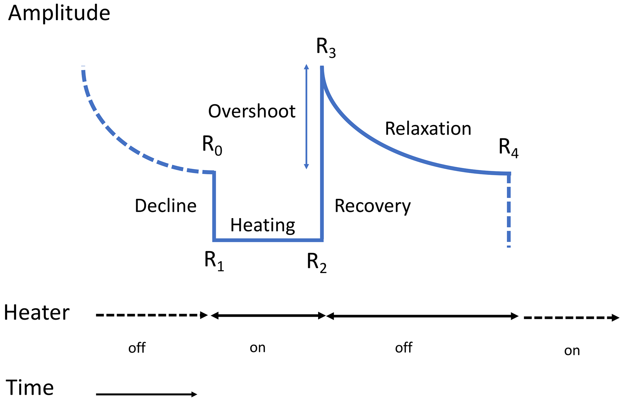
Figure 1 Sketch of the PMSE modulation due to HF heating in a typical overshoot curve; the power amplitudes during different times of the heating cycle are defined.

The amplitudes (R₀, R₁, R₂, R₃, and R₄) marked in Fig. 1 will be considered in our analysis of the observations below, where R₄ is then the start (R₀) of the next subsequent cycle. We follow previous studies (e.g. Havnes et al., 2015) and refer to the curves that describe the measured PMSE during one heating cycle (on and off time) as overshoot curves.

2.1 Decline

R₀ → R₁: As the heater is switched on at R₀, the power effectively falls off instantaneously (depending on the radar frequency used) (Havnes, 2004). The backscattered power drops as the heating enhances the electron temperature and, consequently, the electron diffusivity so that the large electron density gradients are reduced. Therefore, the backscatter is less efficient (Rapp and Lübken, 2000).

2.2 Heating

R₁ → R₂: During the heater-on phase from R₁ and R₂, there are some variations in the power amplitude. Because of the higher electron temperature, the charging electron flux on the dust particles increases during the heater-on period, and often an increase in the power can be seen. The charging timescales become shorter and compete more with the faster electron diffusion (Mahmoudian et al., 2011).

2.3 Recovery/overshoot

R₂ → R₃: The power then increases when the heater is switched off (recovery), and in many cases, the power rises above the previous undisturbed level (overshoot). The electron temperature drops quickly to the initial value before the heater is on due to the highly collisional regime at these altitudes. The dust particles carry a higher charge than before and repel the electrons more strongly. The electrons follow the ion diffusivity, and as a result, the electron density gradients become larger. This causes the backscatter to be larger, creating an overshoot in power.

2.4 Relaxation

R₃ → R₄: Now the power relaxes back to the previous undisturbed level, with a varying relaxation time depending on the conditions. With a long relaxation time, new and undisturbed plasma can enter the radar beam, or the dust present has time to discharge (Havnes, 2004).

3 Observations

We first describe the overall observation conditions, radar operations, and radar analysis, and then we present an overview of the data.

3.1 Overall observation conditions

The presented observations were carried out during the “Mesoclouds 2018” and “Mesoclouds 2020” campaigns in collaboration with UiT Tromsø and IRF Kiruna. The EISCAT VHF radar and the EISCAT heating facility are located in Ramfjord near Tromsø, Norway (69.59^∘ N, 19.23^∘ E). The observations were made on 11/12 and 15/16 August 2018 and 5/6 and 6/7 August 2020, during the night between 20:00 and 02:00 UT. These observations thus represent dusk and night conditions with reduced influence of sunlight on the observational volume compared to other observations, mainly done around noon in June and July.

The solar zenith angles during the observations are in the range of 88–97^∘. PMSEs at 80–90 km altitude are still sunlit but to a lesser extent for most of the previous PMSE observations. To estimate the difference, we compare the solar illumination at the time of our 15 August (2018) observations to those of the summer solstice in the same year. We derive the solar UV flux by calculating the absorption of the solar UV flux by O₂ along its path through the atmosphere (described by Giono et al., 2018). We use solar Lyman-α line (121.56 nm) flux from the SOLSTICE instrument on the SORCE satellite (https://lasp.colorado.edu/home/sorce/data/ssi-data/, last access: 27 February 2020) and O₂ densities from the NRLMSISE-00 atmosphere model (Hedin, 1991) for the location of the EISCAT VHF radar. We estimate that the solar photon flux in August at PMSE altitudes is reduced by at least 1 order of magnitude compared to noon conditions in June, as seen in Fig. 2. This translates to a reduced photoemission current by an order of magnitude. It thus influences the dust-charging conditions since the photoemission current is proportional to the photon flux (Mahmoudian et al., 2018).

Figure 2 Estimated photon flux for the Lyman-α line for 21 June at 12:00 h (UT) and 15 August at 22:00 and 24:00 h (UT) at 85 km altitude. Solar zenith angles used in the estimation included in the label are from the International Reference Ionosphere (IRI) model (2016).

Simultaneous optical measurements of NLCs were done using two cameras located at Kiruna and Nikkaluokta, Sweden (about 200 km south of Tromsø). There was, however, no NLC observation above the radar site, mainly because of weather conditions. During the night of 15/16 August, faint NLCs were observed from Kiruna close to the horizon, approximately above Andøya, i.e., more westward than the EISCAT site. Figure 3a and b shows the temperature profiles (blue line) as measured by the Aura satellite and frost-point temperature profiles (green line) estimated using the Aura water vapor data (both the temperature and water vapor were measured with the Microwave Limb Sounder (MLS) instrument). The height ranges in which the temperature is lower than the frost-point temperature indicate the regions where ice particles can form. This gives a good indication of the conditions present in the atmosphere, showing that the temperatures are cold enough to facilitate ice particle formation at PMSE altitudes. However, there could be variations due to the spatial and temporal differences between the measurements that must be kept in mind. These measurement points were the closest in time and space to the PMSE observations; the horizontal distance to Tromsø is about 490 km in Fig. 3a and about 293 km in Fig. 3b.

Figure 3 Temperature profiles (blue line) as measured by the Aura satellite at 12 and 16 August 2018 and frost-point temperature profiles (green line) estimated using the Aura water vapor data. Latitude and longitude of the measurement points are given in the figures by ϕ and λ respectively.

3.2 Radar operation and data analysis

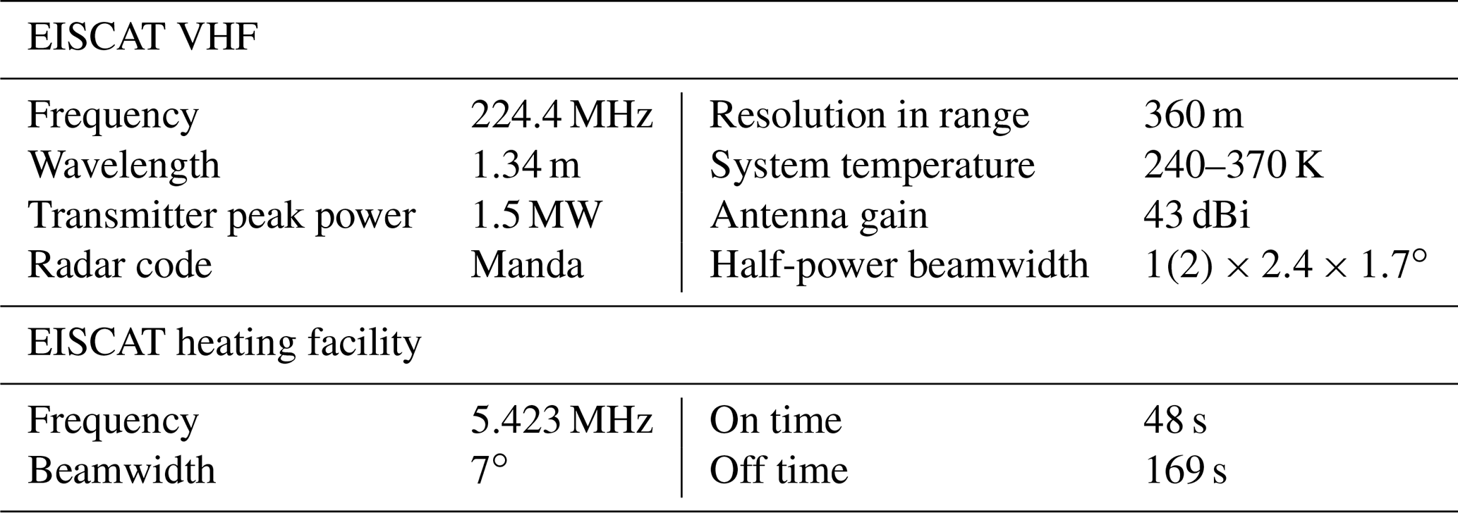
The radar observations were made in the zenith direction with the EISCAT VHF (224 MHz) antennas near Tromsø (69.59^∘ N, 19.23^∘ E). The radar code used was Manda, and reference to EISCAT documentation (Tjulin, 2017) and radar and heating system parameters are given in Table 1. The EISCAT heating facility (Rietveld et al., 1993, 2016) was operated with a vertical beam at 5.423 MHz with a nominal 80 kW per transmitter, which corresponds to effective radiated power (ERP) in the range between 500 and 580 MW, and X-mode polarization was used with a sequence of 48 s on and 168 s off. The vertical extension of the heater beam extends far beyond the region covered by the radar. Given that the vertical winds and velocity fluctuations of the PMSE observed with EISCAT VHF are within a few meters per second and horizontal winds possibly a few tens of meters per second (Strelnikova and Rapp, 2011), the radar at all times measures PMSEs that are influenced by the heating.

A standard incoherent scatter analysis, GUISDAP (Lehtinen and Huuskonen, 1996), was used to derive the radar data products. It provides the electron density derived from the incoherent scatter spectrum assuming that the electron and ion temperatures are equal (which they are not when the heater is on). The backscatter cross section is proportional to $\mathrm{1}/(\mathrm{1}+T_{\text{e}}/T_{\text{i}}+{\mathit{\alpha }}^{\mathrm{2}})$ as is shown by Pinedo et al. (2014), indicating that when the heater is turned on, T_e increases and consequently the backscattered power decreases. The actual electron density is assumed to be not affected, so we use the unit of equivalent electron density as was done previously for observations of polar mesospheric winter echoes (PMWEs) (Kavanagh et al., 2006; Belova et al., 2008) and PMSEs (Mann et al., 2016). The post-experiment integration time used throughout this analysis was 24 s for computational reasons except for one of the observations when we compare with simulations. A resolution of 4.8 s was used. We found that choosing a higher time resolution for the overall discussion did not result in additional information.

Table 1 Parameters for EISCAT VHF radar operation and EISCAT heating facility. Half of the VHF antenna is used for transmitting, and the entire antenna is used for receiving (beamwidth adjusted accordingly).

3.3 Overview of observations

The observations were made from 20:00 to 02:00 UT on four nights in August 2018 and 2020. The observations are displayed in Fig. 4 and shown for the entire period with altitudes from 80–110 km, hence including PMSE and the conditions of the surrounding ionosphere. White vertical areas are observation gaps due to operational problems. We identified interesting measurement intervals in each data set we considered for analysis. A closer look at each area is given in the Supplement, and an overview of the time and altitude range of the areas is shown in Table A1 in the Appendix A.

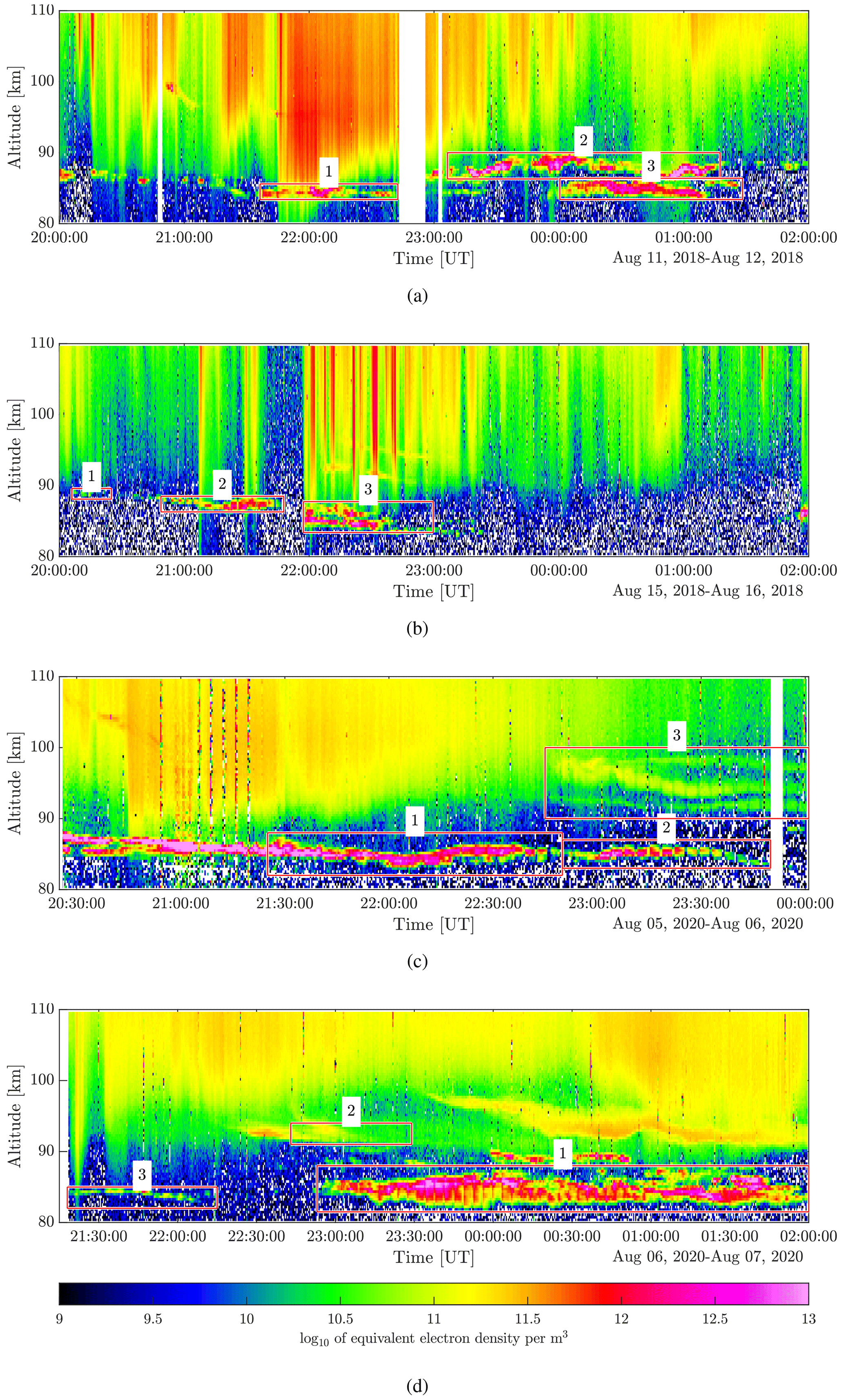
Figure 4 Overview of all four observation days with time intervals and dates given in each respective figure.

3.4 Observation 1: the 11/12 August 2018

PMSE was observed until around 01:30 UT. One can see that the electron densities above and partly below the PMSE are high, showing the typical appearance of particle precipitation. In area 1, the precipitation is strong, and enhanced electron density was observed as low as 80 km, well below the PMSE layer. We considered the following.

• Area 1: PMSE with strong precipitation in the altitude range 83.4–85.6 km from 21:36 UT, lasting about 20 heater cycles;

• Area 2: high-altitude and long-lived PMSE layer extending from 86.3–90 km during about 40 heater cycles, starting from 23:06 UT with some precipitation;

• Area 3: low-altitude PMSE at 83.4–86.4 km from 00:00 UT lasting about 30 heater cycles with some precipitation at the end of the layer.

3.5 Observation 2: the 15/16 August 2018

PMSE was observed before midnight and then again at 02:00 UT. at the end of the measurements. The first observed PMSE (area 1) seems to be not influenced by precipitation. The PMSE observed later (areas 2 and 3) are influenced by moderate precipitation. Modulation is seen in the backscattered power of the lightly ionized portion of the ionosphere from 90–110 km, which can be seen around 20:00–21:00 UT. We considered the following.

• Area 1: high-altitude weak PMSE observed around 20:30 UT at 88–90 km;

• Area 2: PMSE observed from 20:50 to 21:50 UT at 86–88 km, in parts influenced by precipitation;

• Area 3: PMSE from 22:00 UT influenced by moderate precipitation extending over altitudes 83.4–87.8 km during about 30 heater cycles.

3.6 Observation 3: the 5/6 August 2020

PMSE was observed only before midnight. Some observations (areas 1 and 2) show no apparent influence of precipitation. Before the start of area 1, there is PMSE present. However, this is not included in the analysis due to (most likely) direct interference from the heater caused by arcing, which can be seen as vertical lines extending through all altitudes. For completeness, we also consider area 3, which displays a layered structure and is influenced by the heating. The height and the shape suggest, however, that this is not PMSE but rather a sporadic E layer. We considered the following.

• Area 1: strong PMSE in the absence of apparent precipitation for about 1 h from 21:30 UT at 82–88 km;

• Area 2: PMSE at 83–87 km in the absence of apparent precipitation between 22:50 and 23:50 UT;

• Area 3: structure observed above 90 km from 22:45 UT consistent with a sporadic E layer; not included in analysis.

Figure 5 Backscattered power as a function of altitude and heating intervals observed during the night of 5/6 August 2020, in area 2.

3.7 Observation 4: the 6/7 August 2020

From the fourth observation, we see a low-altitude PMSE layer only slightly influenced by precipitation, a second layer at high altitude influenced by heating that also might be a sporadic E layer, and a third area extending over a long period in time and many altitudes that do not seem to be influenced by particle precipitation. We considered the following.

• Area 1: a long interval of PMSE between 81–88 km partly in the quiet ionosphere and partly influenced by precipitation;

• Area 2: sporadic E layer above PMSE height; not included in analysis;

• Area 3: a weak PMSE with little apparent precipitation for about 1 h from 21:30 UT at 82–88 km.

We find, in general, that the overshoot effect disappears in the presence of strong or moderate precipitation, as seen in the 15/16 August 2018 observation in Fig. 4. This is better illustrated in the figures given in the Supplement, where each area is enhanced. At the beginning of the observation campaign on 15/16 August 2018 (area 1), a weak PMSE developed under very quiet ionospheric conditions. The echoes are only weakly enhanced in comparison to surrounding areas, the backscattered power is reduced during heating, and an overshoot is also observed (see Fig. S4).

4 Observed PMSE modulation

First, we discuss two selected cases, one with little or no particle precipitation and one with moderate precipitation. Then we summarize the heating effect and overshoots visible in all the observations, and we discuss these findings in the context of previous observations. Finally, we compare a selected case with simulations of the overshoot cycle and discuss what information we can gain from modulating PMSE with heating.

4.1 PMSE modulation under quiet ionospheric conditions

To discuss PMSE modulation under quiet ionospheric conditions, we chose an area with no apparent energetic particle precipitation; we consider area 2 from the 5/6 August 2020 observation (Fig. 4c). The overshoot curves can be assessed using the overall power plot shown in Fig. 5. The beginnings of new heating cycles are marked with dashed lines when the heater is turned on. The dotted line indicates the time when the heater is turned off again. In many cases, the PMSE signal changes at the heater on and off times and during the cycles themselves. The PMSE layer lies within the altitude range of 83–87 km with a maximum extension of 2 km at its widest. There are clear indications of reduced PMSE power when the heater is on; in many cases, we can see clear overshoots.

In Fig. 6, we have selected two altitude sections for a closer look, altitude 85.2 and 85.6 km, where we can see overshoots in many of the cycles. In general, the overshoots are relatively large, with some an order of magnitude larger than the pre-heater value and with some showing no apparent increase in the PMSE power after the heater is turned off. This seems especially true for the top altitude where the PMSE power is at its highest, the lower height has a somewhat lesser PMSE power, and more overshoots are visible. The decline is visible in many of the cycles and is very strong for cycles 40–47. One can also see that characteristics of decline and overshoot often change between adjacent heating cycles and height intervals, e.g., in heating cycle 41.

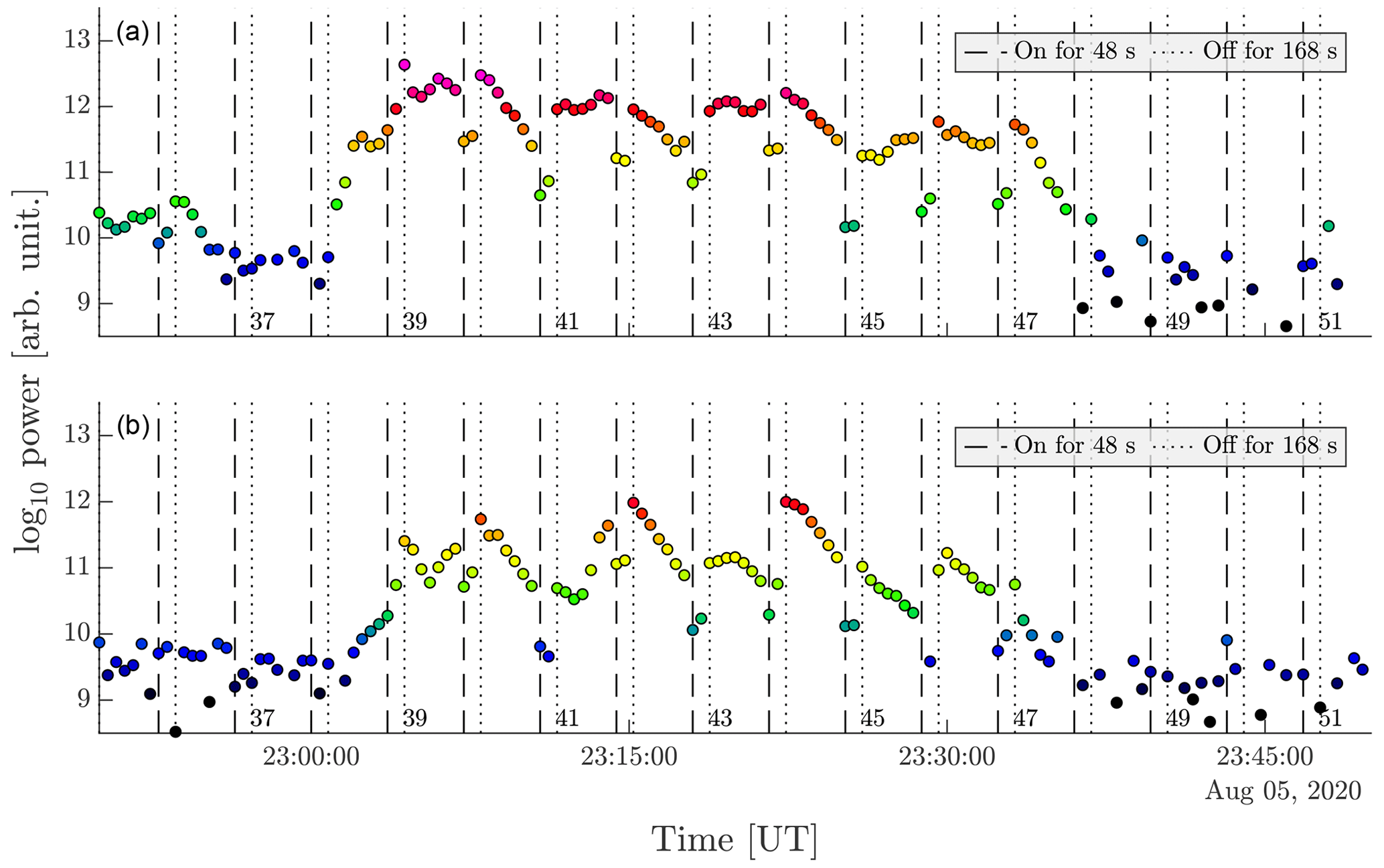
Figure 6 Backscattered power at altitude 85.2 km (b) and 85.6 km (a) and heating intervals observed during the night of 5/6 August 2020 in area 2. The color of the dots follows the color scale of Fig. 5.

For a closer investigation, we describe the ratios of the amplitudes during the different phases of the heating cycle. The different power amplitudes are marked in the overall sketch given in Fig. 1. The different amplitudes observed during the heating cycles are plotted in Fig. 7, where the amplitude ratios are considered. We find that during most heating cycles, the signal drops when the heating is switched on (decline R₁ < R₀, Fig. 7a).

We assume that the observed signals are PMSE when R₀ > 10^10.5 (which corresponds to around 3.16×10¹⁰; Ullah et al., 2019), and one can see that in most cases that do not meet this requirement; there is no PMSE modulation visible. However, as we will see later, this condition removes a few instances of low-power modulated PMSE with large overshoots. The same can be said for the green points that show a decline but are below the threshold. They could be showing a decline but also be noise due to random fluctuations from the two measurement points.

Figure 7 Comparison of the power amplitudes observed on 5/6 August 2020, area 2.

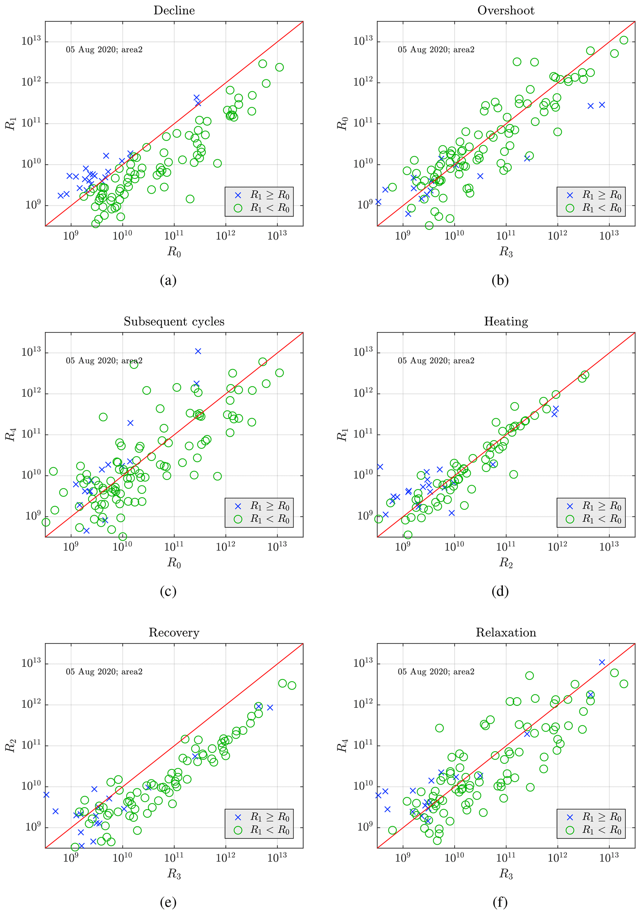
The ratio of the amplitudes R₀ and R₃ describes an overshoot (R₀ < R₃), and this comparison shows that overshoots and undershoots are equally abundant, independent of the signal strength (Fig. 7b). Comparing the signals at the beginning of subsequent cycles (Fig. 7c) shows no trend and a broad range of values which suggests variation either due to ionospheric conditions or due to neutral turbulence (rather than dust).

One can see in Fig. 7d that for strong signals the amplitude stays constant or decreases slightly during the heater-on phase. The change in amplitude during the heating can indicate the charging process of the dust particles, where the faster timescale of diffusion or dust charging dominates (Mahmoudian et al., 2011). According to Havnes et al. (2015), large PMSE structures can cause the diffusion timescale to be longer and, consequently, have a quicker and larger increase in power during the heater-on phase. The comparison of R₂ and R₃ in Fig. 7e describes to what extent the signal increases again when the heater is switched off. This increase is seen in most cases except for the small amplitudes, which might be either low-power PMSE or random fluctuations.

Finally, in Fig. 7f, the ratio of R₃ and R₄ describes the signal after the heater is switched off (relaxation). One can see a broad scatter symmetrically around the diagonal, indicating that the natural variations in the PMSE power are dominant. Any relaxation after heating is difficult to discern from this since their contribution could disappear due to a significant background increase in PMSE power. This is due to the considerable period between the two points (168 s), which according to Havnes (2004), is enough time for the ionosphere to change or dust to become discharged, whereas 48 s used for the on time is not.

We compile these results in histograms of the amplitude ratios (Fig. 8). The histograms contain only cycles with a value R₀ > 10^10.5 of the PMSE amplitude before the heater is turned off to only include those with PMSE and exclude the cycles that contain noise or are mostly noise. We only include those cycles that show a decline due to heating in all the histograms. In Fig. 8a, we see that 55 % of the ratios are smaller than 1 and thus show a decline (affected by the heater) and that the average value of those ratios that are below 1 is 0.72. This is a reduction of 28 % of the pre-heater value on average when the heater is turned on. We have the overshoot in Fig. 8b. Only 10 % of the cycles show an overshoot with an average value of 0.44. Even though there are not many overshoots for this observation, those observed show an average reduction of more than half, indicating very large overshoots. Figure 8c shows that most (95 %) of the observations show a decrease in power while the heater is on. Figure 8d shows that 66 % of the cycles show an increase in power when the heater turns off, which is similar to the number of cycles that show a power reduction when the heater is turned on. Then in Fig. 8e, we see a general increase in power from cycle to cycle. Thus a general decrease to pre-heater value cannot be determined, most likely due to increasing background PMSE dominating the signal and the histogram, where 87 % of the cycles show an increase in power in subsequent cycles. This can be related to why we see so few overshoots in this observation, and that increase in PMSE power is significant for many of the cycles. The overshoot disappears due to background variations.

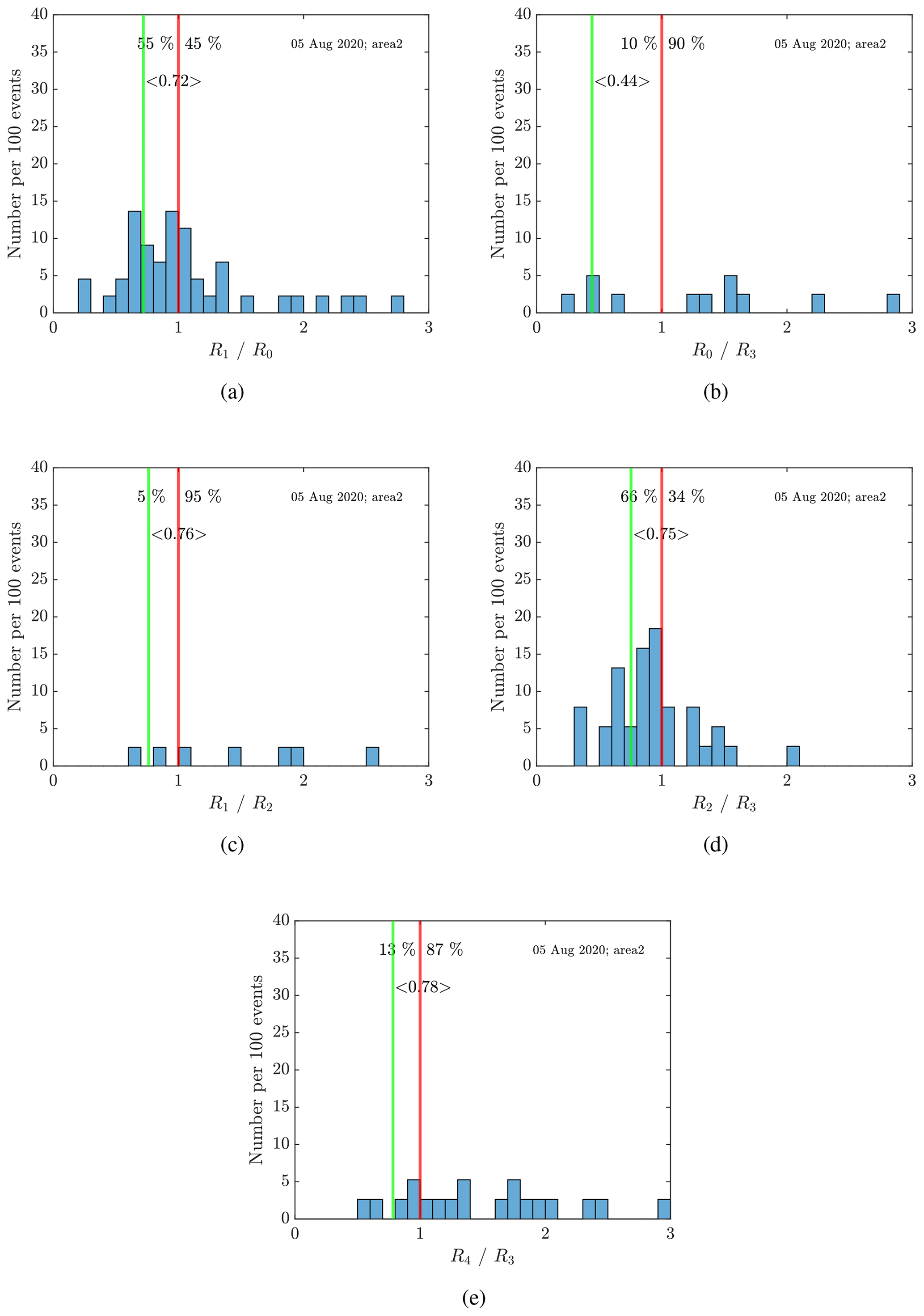
Figure 8 Average of (a) decline, (b) overshoot, (c) heating, (d) recovery, and (e) relaxation for the observed data on 5 August 2020 in area 2. Only overshoot curves with a minimal background amplitude of R₀ > 10^10.5 are considered. The ratios are chosen so that if we observe an overshoot curve like shown in Fig. 1, all ratios are smaller than 1. Thus, the histograms are clipped at a maximum ratio of 3. The green line and the corresponding number display the mean for all ratios smaller than 1.

4.2 PMSE modulation during moderate particle precipitation

Conditions with moderate particle precipitation are observed in area 2 of the observation from 15/16 August 2018 (see Fig. 4b). The overall power plot is shown in Fig. 9. As discussed above, some heating intervals have noticeably very strong overshoots (14, 15, 16, 17). One can note that the influence of the heating is most pronounced at the beginning and the very end of the observation interval when there is no apparent particle precipitation. Precipitation occurs in cycles 18 and 19 and then in cycles 24 and 25. When the heater is switched on, there is no reduction in power, and the precipitation dominates the received signal for all altitudes in these cycles. The power plot for two selected height intervals shown in Fig. 10 shows this in more detail, where the modulation entirely disappears in the cycles influenced by precipitation. This is to be expected and has been shown before. One of the reasons why the modulation disappears in the PMSE layer is that the atmosphere below the layer is ionized due to the strong precipitation, and the HF radio wave might be strongly absorbed before it reaches the PMSE layer and thus not be strong enough to heat the electrons appreciably in the layer.

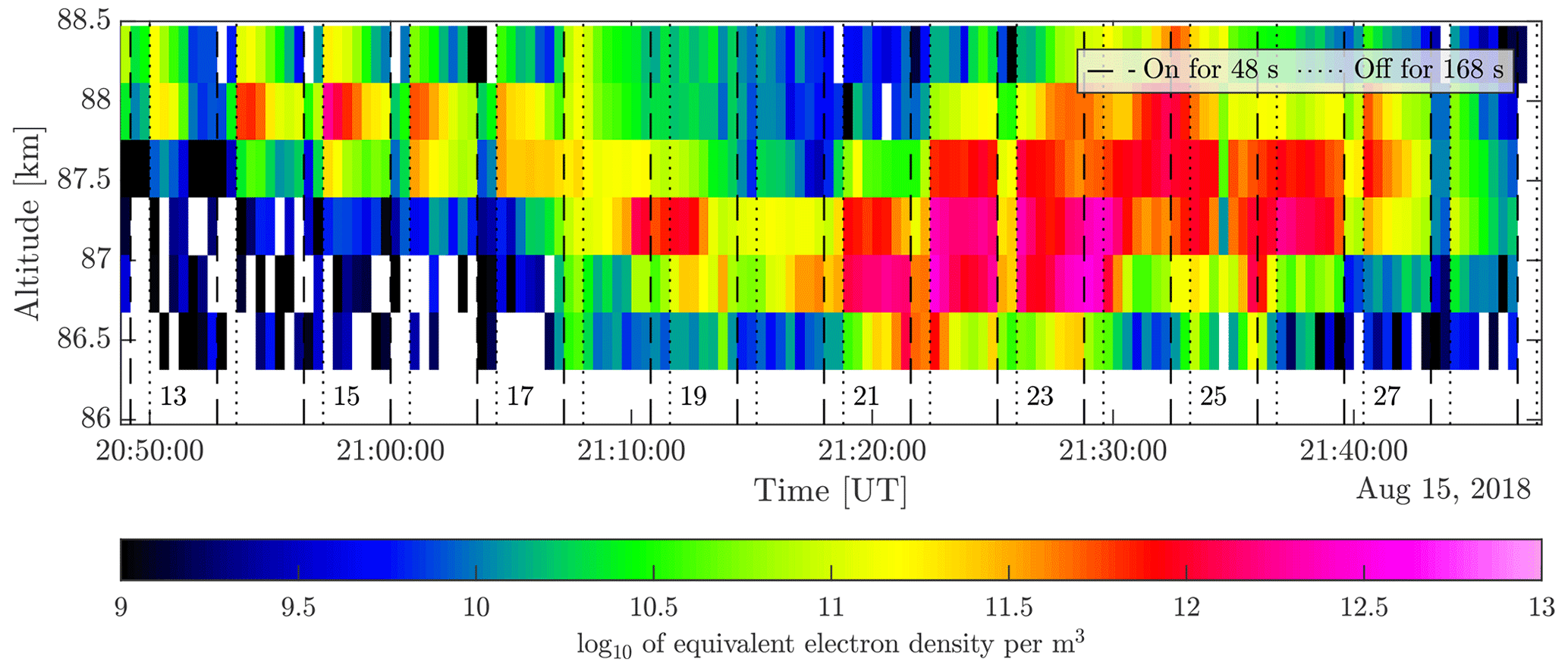
Figure 9 Backscattered power as a function of altitude and heating intervals observed during the night of 15/16 August 2018, in area 2.

The different amplitudes observed during the heating cycles in this area are plotted in Fig. 11. We find that during most heating cycles, the signal drops when the heating is switched on (decline, Fig. 11a). The cases that show no decline are spread over all amplitudes, indicating the cycles that might be influenced by precipitation and thus might show an increase in power when the heater is on. The overshoots and undershoots are equally abundant independent of the signal strength (Fig. 11b). As observed in the area discussed above, there is no trend when comparing the signals at the beginning of subsequent cycles (Fig. 11c). The change of amplitude during the heating (Fig. 11d) is small for most observations.

In most cases, the amplitude increases (Fig. 11e) when the heater is switched off, similar to the heated cycles, which is to be expected. Finally, in Fig. 11f, the ratio of R₃ and R₄ describes the relaxation, showing a large spread around the diagonal with somewhat more observations showing a reduction. This large spread can be attributed to the ionospheric variability due to the large timescale of the off time, as was mentioned previously.

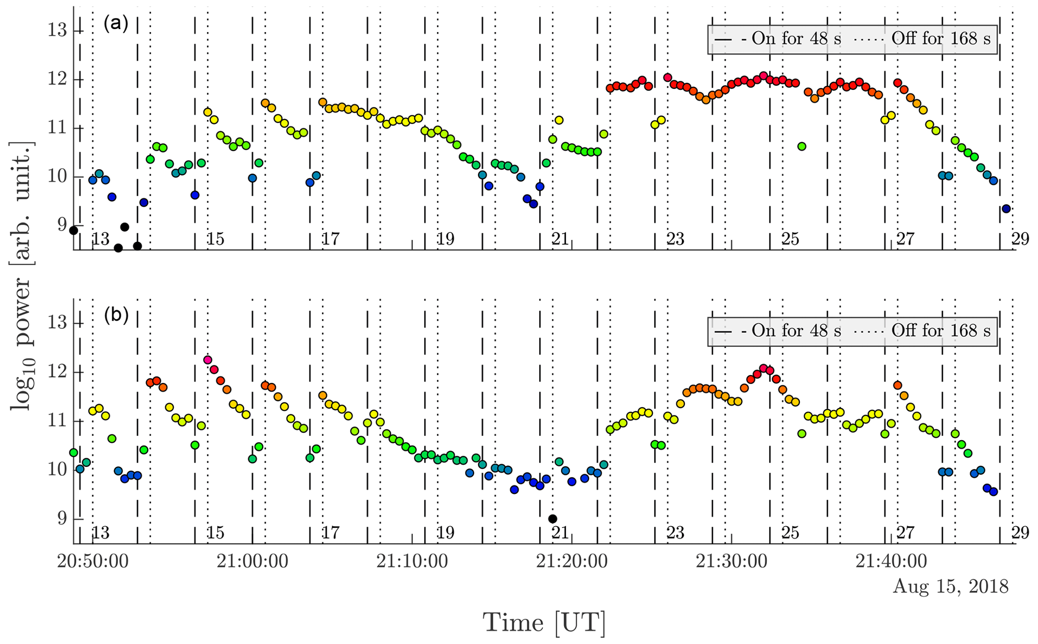
Figure 10 Backscattered power at altitude 87.4  km (b) and 87.8  km (a) and heating intervals observed during the night of 15/16 August 2018 in area 2. The color of the dots follows the color scale of Fig. 9.

The histograms of the power amplitudes are shown in Fig. 12 with the same criterion as before (also given in the figure text). Here the overshoot is seen in 55 % of the cycles with an average of 0.75 decline ratio (Fig. 12a), similar to the previous observation. Here the overshoot is seen in 31 % of the observations with an average of 0.64 overshoot ratio (Fig. 12b), which is more than the previous observation, even with precipitation. Similar to the previous observation, when the PMSE power increases (and is not influenced by precipitation), we see an influence of the heater but not an overshoot (or a minimal overshoot). For the cycles with a lower PMSE power (like in cycle 15), the overshoot is large, but the background PMSE power is lower; thus, the overshoot is easy to see. During the heating, there seems to be a general decrease in the values, with 76 % of the values showing a decrease during the heater-on phase (Fig. 12c). The recovery (Fig. 12d) ratio shows that 58 % has an increase in power when the heater is turned off, showing similar values to those for when the heater is turned on (decline). Then there seems to be a little over half of the cycles that show a general increase in pre-heater values between cycles (Fig. 12e).

Figure 11 Comparison of the power amplitudes observed on the 15 August 2018 in area 2.

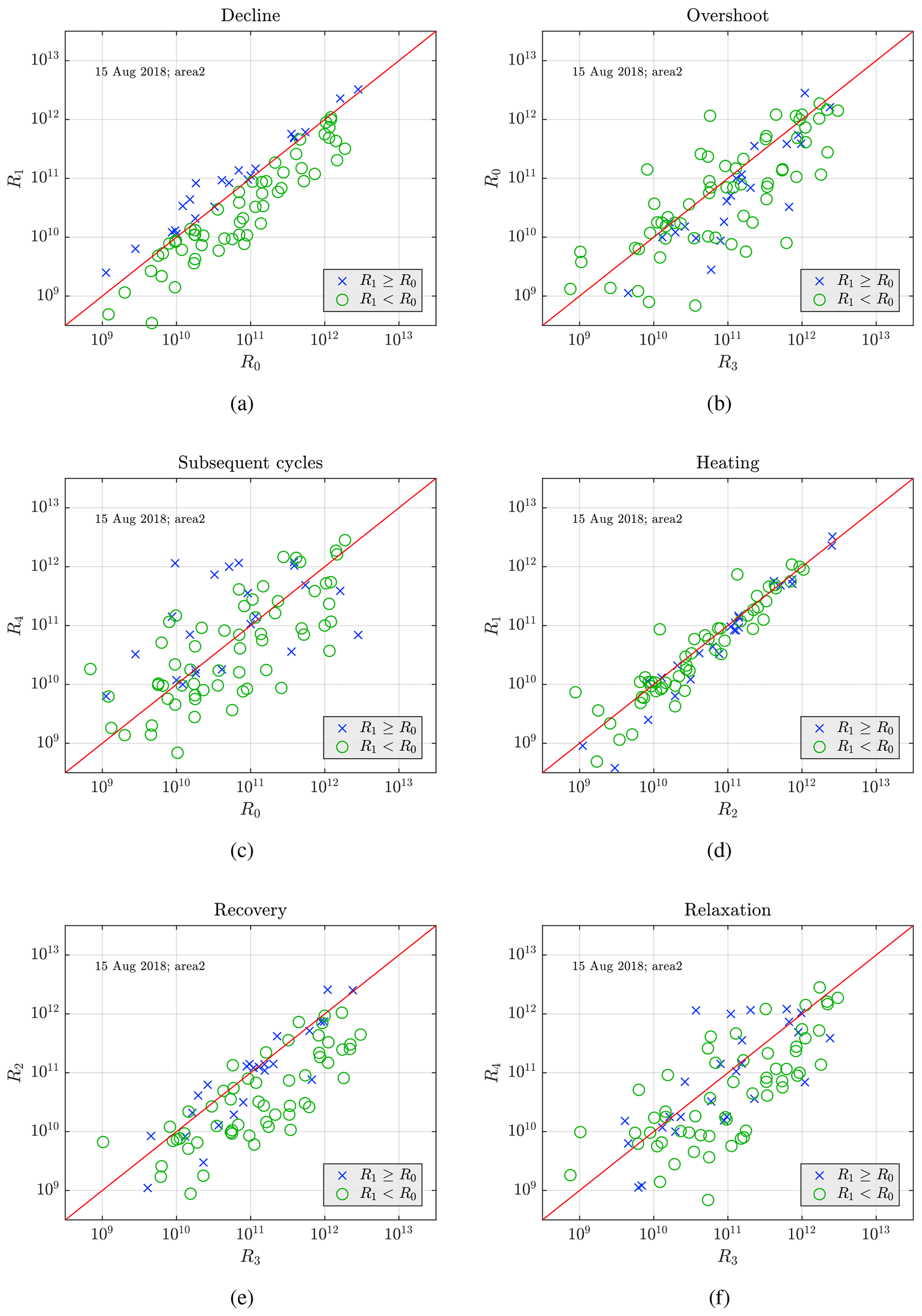
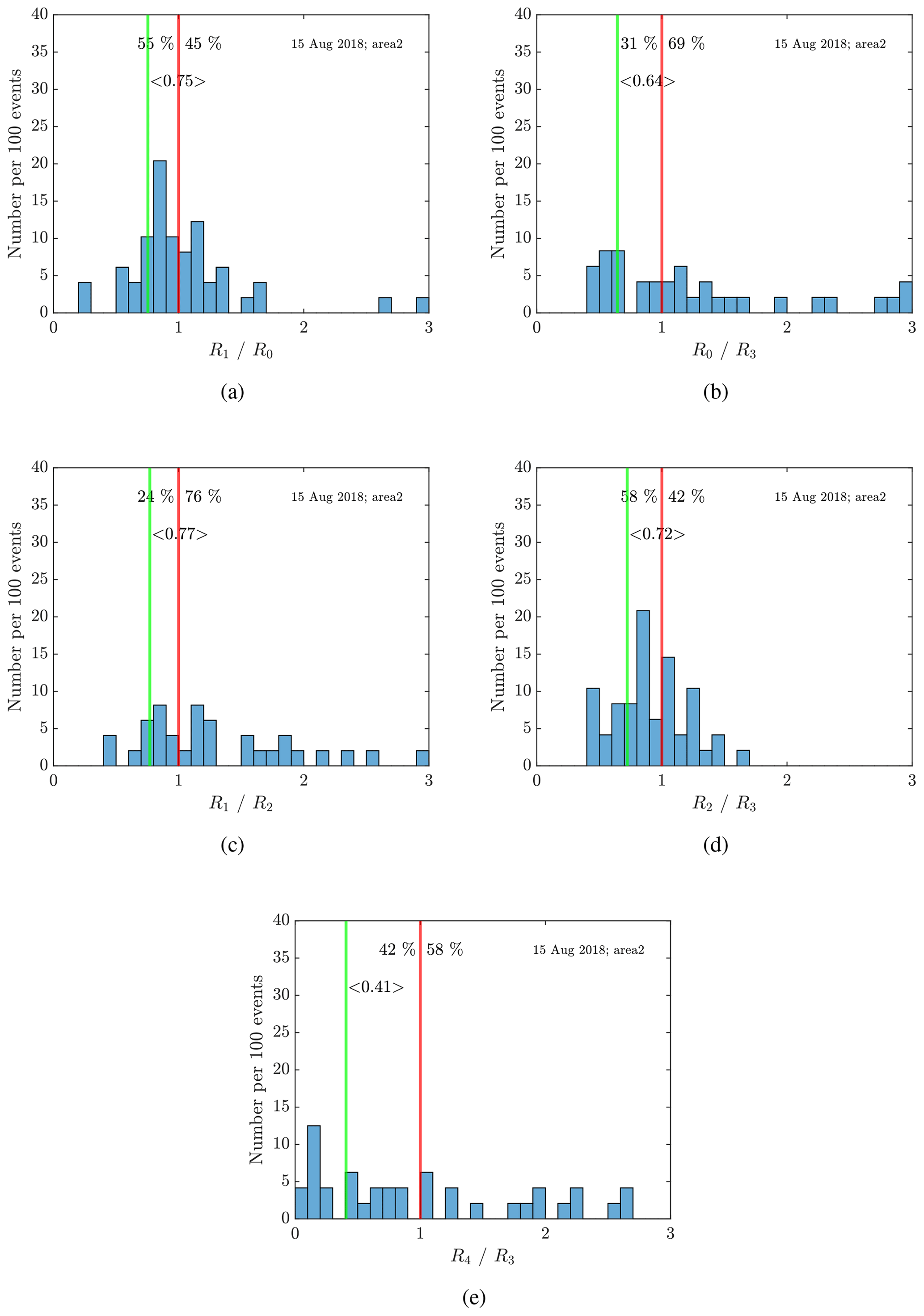
Figure 12 Average of (a) decline, (b) overshoot, (c) heating, (d) recovery, (e) relaxation for the observed data on 15 August 2018 in area 2. Only overshoot curves with a minimal background amplitude of R₀ > 10^10.5 are considered. The ratios are chosen so that if we observe an overshoot curve like shown in Fig. 1, all ratios are smaller than 1. Thus, the histograms are clipped at a maximum ratio of 3. The green line and the corresponding number display the mean for all ratios smaller than 1.

4.3 Overall observational discussion

Here we summarize, in Table 2, the decline and overshoot ratios for all the observations (see Figs. S27–S36 in the Supplement for reference). In general, the heating effect is seen in more than half of the heating cycles for each respective area, with most of the average ratios showing values close to 0.75. These calculations show only the observations with a value of R₀>10^10.5 to indicate the presence of PMSE and exclude noisy data.

This, however, causes the faintest PMSE to be excluded from the histograms, as is seen for the overshoot ratio for area 1 from 15 August 2018; here, the PMSE power is below the threshold. Thus no cycles are included in the calculation despite 100 % of the cycles showing a decline due to heating. This would suggest manually inspecting low-power PMSE influenced by heating would be a better option or introducing other criteria to include these.

Table 2 Summary of histogram results (see histograms (Figs. S27–S36) in the Supplement) for the decline (R₁ $/$ R₀) and the overshoot (R₀ $/$ R₃) ratio when they are smaller than 1 (indicating heating effect and overshoot) for all four observations. These numbers only include observations with minimum background amplitude R₀ > 10^10.5. A1 refers to area 1 for that observation's date and so forth.

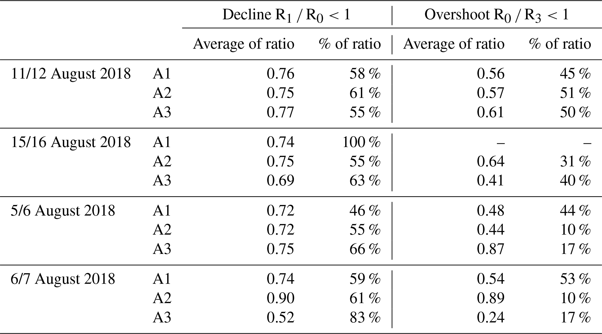
To summarize, we see only overshoots in less than half of the cycles, with many cycles often more influenced by background ionospheric conditions that might overshadow the heating of the PMSE. Ullah et al. (2019) show a more significant occurrence of overshoots in their observations, with around 40 %–70 %, where their observations were during daytime. Havnes et al. (2015) observations had a much larger ratio of cycles with decline present and a slightly higher percentage of overshoots present.

However, in our case, we see a few instances where the overshoot in some cycles is unusually large. Myrvang et al. (2021) found that a higher electron temperature due to heating could be achieved during nighttime compared to daytime, which might help explain some of these large overshoots. However, Kassa et al. (2005) found for their observations that the heating temperature effect observed increased for the observation with the most amount of sunlight (near noon).

Other possible reasons for unusually large overshoots could be a change in the PMSE/NLC season, as is noted by Latteck et al. (2021), when the season is getting longer. Since our observations are in reduced sunlight and close to the end of the season, more varying background conditions might influence our observations than those during the day in June/July.

4.4 Comparison of a selected observation to simulation

Here we take a closer look at the approximately 1 h time interval, which is marked as area 2 in the observation from 15–16 of August 2018, shown in Fig. 13; the data cover the heating cycles 12 to 27 and range over seven height intervals of around 360 m each. The ionosphere is influenced by precipitation in cycles 18 and 19 and then again in cycles 24 and 25, and there are no overshoots present in those heating cycles, as mentioned before. The PMSE in intervals marked with A, B, and C in the figure shows a decrease when the heater is on and overshoots when the heater is turned off. Interval A shows relatively low PMSE power but quite high overshoot curves compared to intervals B and C, as we will investigate further.

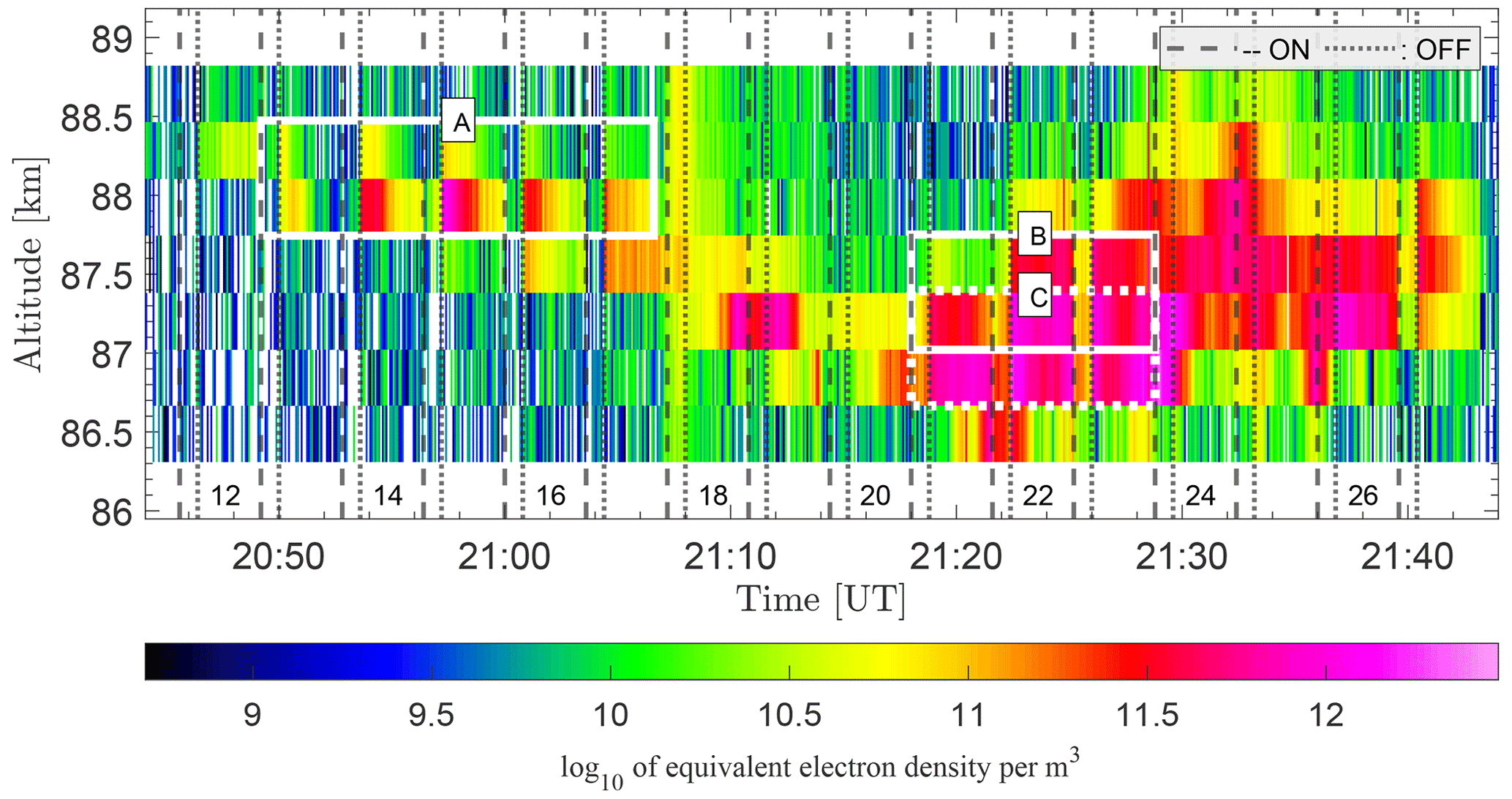
Figure 13 Overview of Area 2 – 15 of August 2018, with interesting visible overshoot cycles marked with intervals A, B, and C. Data resolution is 4.8 s. Cycles are marked in the figure (from 12 to 27) as well as their corresponding On/OFF period.

Individual heating cycles are shown in Fig. 14a for both altitudes from interval A, with PMSE power and measurement error provided by the EISCAT GUISDAP analysis. The corresponding average overshoot cycle for the respective altitude is shown on the right in Fig. 14b; in blue is the corresponding average overshoot cycle for the respective altitude. As can be seen, the overshoot is relatively strong for many of the heating cycles, especially the strong overshoot seen in cycle 15 for both altitudes with relatively high but decreasing overshoot on both sides of the cycle. Note the two y-axis scales for the different altitudes, where the heating cycles from altitude 88 km have such a low background PMSE power that the scale is an order of magnitude lower than the altitude below. Both altitudes have relatively low background PMSE power compared to intervals B and C, with the PMSE at 88 km altitude barely present or the irregularities on the limit of being seen by the VHF radar. It is thus interesting to find such large overshoot cycles for this particular interval.

Individual heating cycles from intervals B and C are shown in Fig. 15a with their corresponding altitude average on the right-hand side in blue (Fig.15b; note that here the y-axis scale is the same for all the altitude ranges). They cover heating cycles 21, 22, and 23. The overshoots are present for the lower altitudes but are not as high as in interval A. However, the overshoot does not decline evenly but increases again before reaching the initial signal level. This influence can be seen in the averaged heating curve for altitude 86.7 km, where after about 120 s, the power starts to increase again. This is either because of the beginning influence of particle precipitation on the ionosphere or variation of the PMSE structure due to the long relaxation time (Havnes et al., 2015). This influence is very strong in the subsequent cycle (cycle 24), where the PMSE power increases during the heater-on period. This type of ionospheric variation can influence the observations to the extent that heating effects are less visible. In the same time interval (intervals 21, 22, 23) at the altitude above, the overshoots are small, especially for the first cycle (21), while the PMSE power is relatively low. This is in contrast to the observation made at the higher altitude in interval A where a significant overshoot is observed at low PMSE power. This might indicate that there are different conditions at play for these two cases. Havnes et al. (2015) has mentioned that higher altitudes of PMSE reside in more turbulent conditions, thus a more significant variation in cloud structure and a longer relaxation time after heater turn-off time as a result.

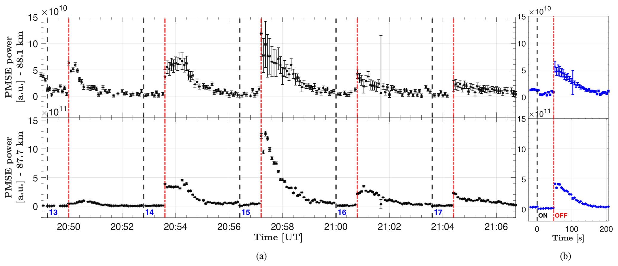
Figure 14 Individual overshoot curves (a) from interval A (from Fig. 13) shown with their corresponding altitude average on the right-hand side (b). Heating cycle numbers are shown at the bottom, and the on-and-off period for the averaged cycles is also shown. Note that the y-axis scale for altitude 88 km is an order of magnitude smaller than for the altitude 87.7 km.

A comparison of the average overshoot curves for each interval (A, B, and C) is shown in Fig. 16a and their corresponding normalized average curves in panel (b). The values are normalized to the initial PMSE power taken as the average of the last five values (24 s) before the heater is turned on. This is chosen to have sufficient data when some measurement points are missing and to better compare to the rest of the data used in this article which are at a resolution of 24 s. Data were normalized after averaging the cycles from each interval. We can see that the highest normalized overshoot (b) is the one from interval A, which has the lowest background PMSE power (a) and that the lowest normalized overshoot is from interval C, which has the corresponding highest PMSE background power. This high PMSE power is possibly due to an onset of precipitation which becomes apparent in the subsequent cycle 24 right after intervals B and C.

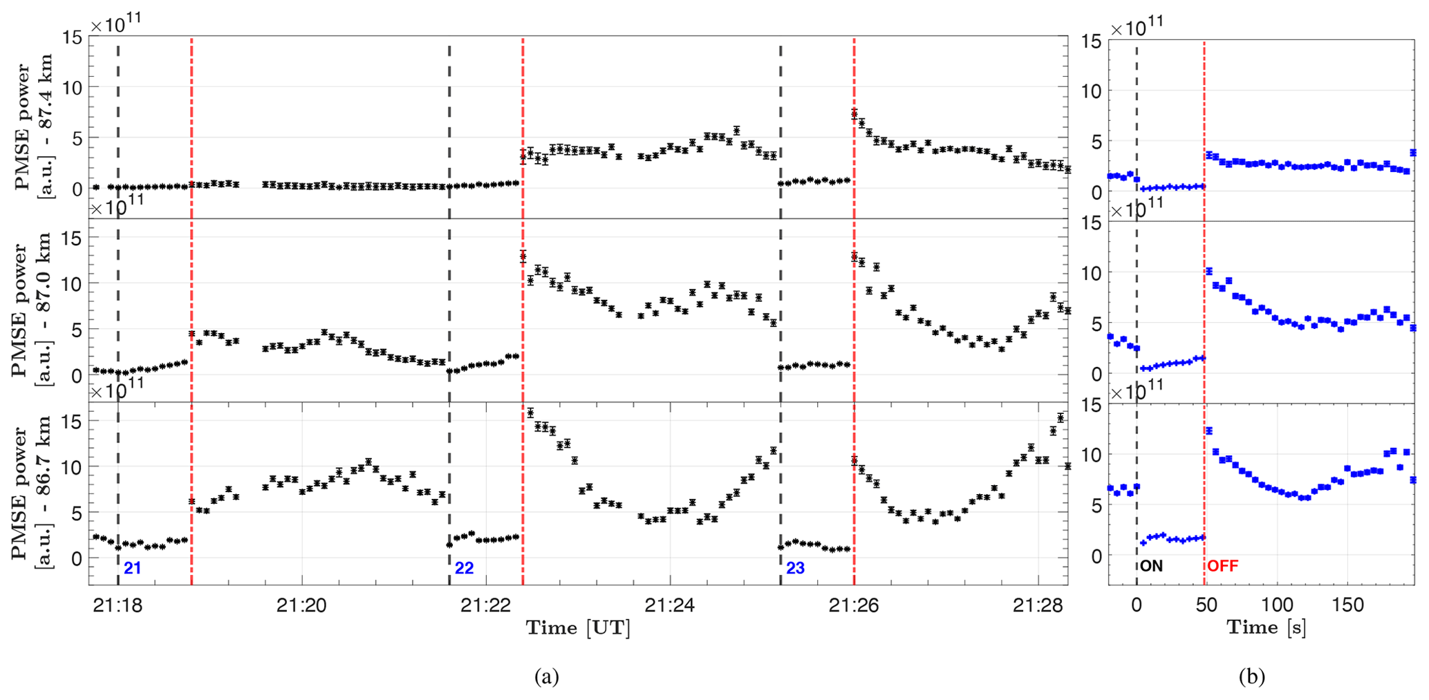
Figure 15 Individual overshoot curves (a) from intervals B and C (from Fig. 13) shown with their corresponding altitude average on the right-hand side (b). Heating cycle numbers are shown at the bottom, and the on-and-off period for the averaged cycles is also shown.

We compare these selected overshoot curves to a computational model initially developed at Virginia Tech. It treats the plasma as a fluid including an arbitrary number of charged particles, neutral particles, and dust particles; the dust charging is described in the orbital-motion-limited (OML) approach (see, e.g., Scales and Mahmoudian, 2016). The model's parameters include the electron diffusion time scale, the charging time scale, and the time evolution of electron and ion densities. The dust charging causes electron density depletion, and the amplitude of electron density fluctuations determines the radar backscattered amplitude. The simulations assume an initial plasma temperature of T_i=150 K and a background electron density of 2×10⁹ m⁻³. Which fits well with the same parameters derived from the IRI model (2016) for the time and date of the observation. The simulation also assumes a reduced photoemission rate used in the charging equations in line with the experiments being done for conditions with low photoemission.

The resulting simulated overshoot curves are shown in Fig. 17b and for comparison are the averaged and normalized observations from intervals A, B, and C (marked in the same color and symbol as previous figures) shown on the left. The simulations best fit to the observed overshoot curves for 3 nm dust particles. However, there is little difference for similar sizes of dust (e.g., 3–4 nm). This result fits well with the altitude range we measure the observed PMSEs since, in general, we can assume to find smaller particles of dust at higher altitudes (however subject to neutral air movement) as well as the fact that there were no NLCs observed and thus the particles were not optically visible (larger >20 nm).

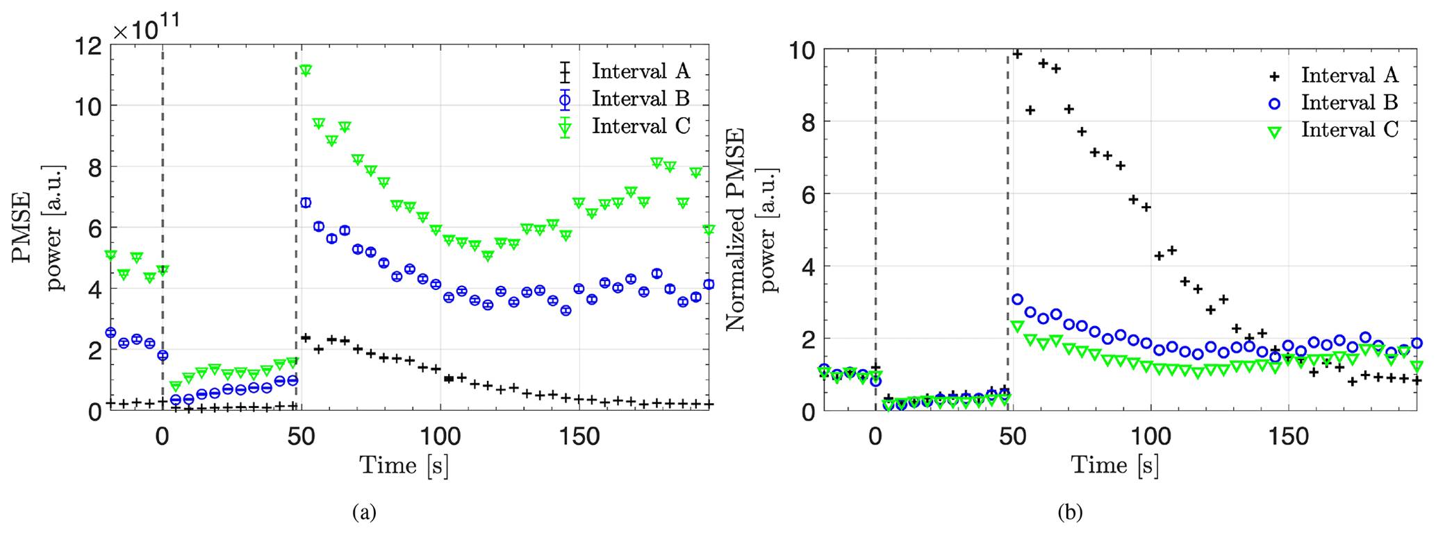
Figure 16 Average overshoot curves for each respective interval (a) and normalized average overshoot curves (b) for the same intervals. They are normalized with the average of the last five values before the heater was turned on.

The normalized and averaged data from interval A has a higher overshoot than the simulations can produce, where the simulation has an overshoot of around 8.4. At the same time, the observations show an overshoot of almost 9.9. The timescale of the simulation for interval A runs for 300 s, while the observation has a much quicker equalization toward the “background” PMSE value/undisturbed plasma values. For the simulation to reach such a high overshoot, the ratio between dust and electron number density is only at 35 %, and with a heating ratio increase for electron temperature of 8 times the pre-heater value. This would indicate that the dust density is lower than for the other two intervals and that the heating effect is consequently larger. As discussed later, the electrons gain a higher temperature, and charging onto the dust particles is, therefore, more effective, where some dust particles can gain more than a single charge.

A comparison of observations for intervals B and C and their corresponding simulations show a better agreement where the overshoot and relaxation are very similar. For these overshoots to be produced in the simulation, the ratio of dust to electrons must be higher, with 60 % for interval B and 68 % for interval C. The increase at the end of the relaxation period for both intervals is not reproduced in the simulations; this is assumed to be due to the influence of the precipitation that occurs clearly in cycle 24 and is already increasing the background PMSE power in the previous cycles. Compared to the observations, the simulated signals drop slower during the heater-on phase and rise more slowly to the overshoot when the heater is switched off again. The measured response of the PMSE to the heating is instantaneous within the 4.8 s resolution of the data. A possible explanation for this difference is that the numerical model might have missing parameters or processes to simulate this increase. This is in contrast to the decrease we see in most observations, as was discussed previously.

On the left-hand side in Fig. 18a, we can see the average charge number found for the simulation for each respective interval (marked in the figure). For interval A the average charge number reaches a maximum of about 1.38 charges per dust particle during the heater-on phase. This indicates that to achieve such a high overshoot, the charging efficiency of the dust particles needs to be high and that (due to high electron heating temperature) many dust particles will gain more than one negative charge during the heating cycle. Note the longer timescale shown in the simulation for interval A (300 s), indicating that it takes longer for the overall average charge on the dust particles to equalize back to pre-heater values. As was mentioned before, the dust population is much lower for interval A compared to the other two intervals since the ratio of dust to electrons is lower. Consequently, the significant increase in temperature (by a factor of 8) causes a larger average charge number on the dust particles during the heater-on phase. For the other intervals (B and C), the maximum average charge number is less than one during the on phase of the heater for both cases, with interval B being around 0.9 charges per dust. For interval C, the average dust charge lies at about 0.86. This corresponds well with the observed and simulated overshoot curves from Fig. 17, where the higher overshoot is observed in interval B. Thus the average charge number is consequently higher. So the effective charging of the dust during the heater-on phase for these intervals is less than for interval A, and a smaller overshoot is observed.

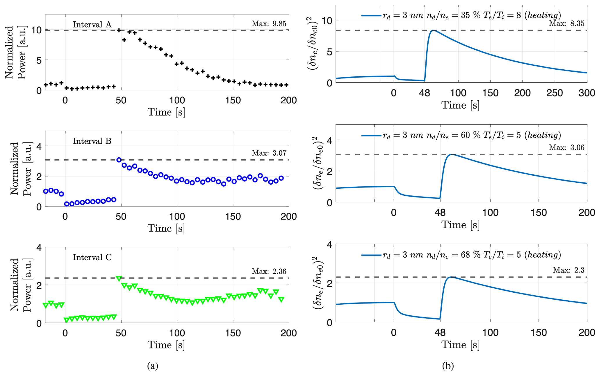
Figure 17 Comparison of the averaged and normalized heating cycles for each interval (a) to its corresponding simulation of the overshoot cycles (b). Note the longer timescale of simulation of interval A (longer time needed for simulation to return to equilibrium).

On the right-hand side in Fig. 18b, we have the ratio of the diffusion time to the charging time scales for each respective interval. Here we can see the variation between the two timescales and how this changes during the heating cycle. For all the intervals, there is an increase in the ratio when the heater turns on, a relaxation during the heater-on period, a sharp increase when the heater is turned off, and a slow decrease during the heater-off period. The significant increase in the heater-on time could be understood as the charging timescale becoming smaller with increased electron charging onto dust particles due to the increased electron temperature. This corresponds well with the increased average electron charge on the dust particles seen in Fig. 18a. Here the average dust charge is highest for interval A, and the ratio of timescales is also highest for this interval, which might indicate a faster charging timescale for that interval than for the other two. The increase at heater turn-off time is also due to a decrease in the charging times; more dust is being charged now by the ion portion of the plasma, which drags the electrons along and causes the observed overshoot. Thus for interval A the simulation of the overshoot curve fits best with a lower ratio of dust particles to electron density. Therefore we might argue that there is more plasma than in the other two intervals. This larger plasma population might then charge the dust more quickly, causing a smaller charging timescale and, consequently, a larger overshoot in interval A.

Another difference could arise in the diffusion timescales in the respective intervals. The diffusion timescale is proportional to the ion-neutral collision frequency, which decreases with decreasing neutral density. Hence in interval A at a higher altitude and with lower neutral density, the diffusion timescale can be shorter than in the other interval (Havnes et al., 2015). The estimated ion-neutral collision frequencies are given in Table 3, which are derived using neutral density from the NRLMSISE-00 atmosphere model (Hedin, 1991).

Table 3 Neutral density for each interval from NRLMSISE-00 atmosphere model (Hedin, 1991) taken at 21:00 UT and the estimated ion-neutral collision frequency (see Ieda, 2020; Cho et al., 1998).

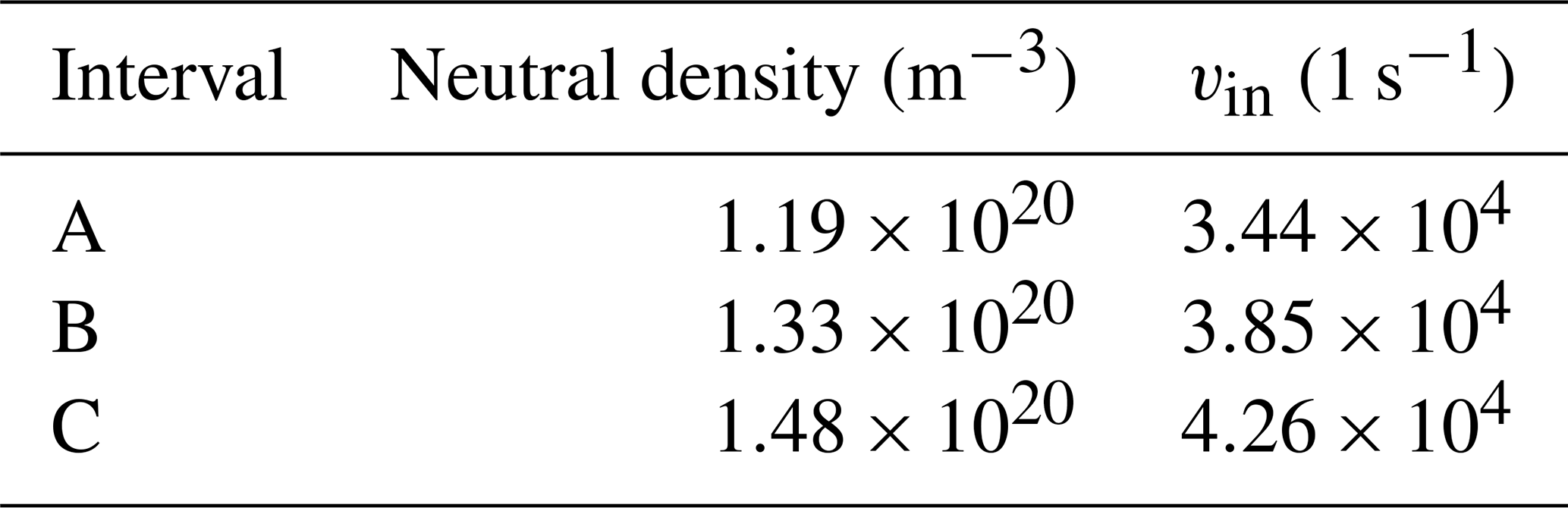
The timescale that is the fastest is the dominating one. So when the heater turns on, the diffusion timescale might be lower for interval A. So when the heater is turned on, the diffusion timescale decreases even more due to its dependence on the temperature ratio ($T_{\text{e}}/T_{\text{i}}$), and we expect/need a more significant temperature increase for the electrons in interval A to explain such a large overshoot. As the heater is turned on, the charging timescale decreases due to the increase in electron temperature. A larger charging effect is seen in the interval A simulation (average charge number) compared to the other intervals. Consequently, a larger overshoot is seen.

So to summarize, the decreased diffusion timescale for interval A due to reduced neutral density and the significant increase in electron temperature combined help explain the large overshoot seen for interval A. The higher electron temperature could be explained by greater absorption of the heater's energy in the interval. According to Havnes et al. (2015), the amount of electron density per altitude will determine where the heater's energy is absorbed and how much. This generally causes lower altitudes of PMSE to become more heated than higher altitudes. Interval A is at a higher altitude than the other two intervals. Still, the precipitation present in cycle 18 before intervals B and C could cause the altitude regions below these intervals to have a higher electron content and, thus more absorption of the heater's energy below.

5 Discussion and conclusion

For the presented observations, we find that artificial heating affects the PMSE signals during less than half of all the observed heating cycles with a pre-heated PMSE power R₀>10^10.5; the average reduction of the power is about 25 % from the pre-heated value. The cutoff, R₀>10^10.5, excludes cycles that do not show PMSE and cycles being highly influenced by noise. With this criterion, we covered most of the PMSE. However, some very faint ones were excluded, and some were affected by heating and showed large overshoots. We find that the heating has little effect on PMSE during ionospheric conditions with particle precipitation which other authors also see. This is especially so for strong and moderate particle precipitation. We assume that under these conditions of higher ionization, the heating waves are mainly absorbed in lower altitudes, thus not causing a heating effect in the PMSE layer. Often the background ionospheric conditions strongly influence the PMSE profile during one heater cycle, and it is thus challenging to derive a correct relaxation time, which would be an interesting parameter because it depends on the dust conditions present in the layer.

Figure 18 Simulations of average dust charge number on (a) for each respective interval and the ratio between the diffusion time and the charging time scales for the same intervals on (b).

As to the shape of the PMSE modulation curves, the variation of the PMSE during the heater-on period (from R₁ to R₂) is affected by two competing processes: the charging and the diffusion. For the presented observations, most heating cycles display a signal decrease from R₁ to R₂. Less than half of the cycles influenced by heating show an overshoot when the heater is turned off. However, observed overshoots are generally high and, in some cases, very high. These high overshoots could be attributed to the dust charge in the presented observations being more strongly influenced by heating, as the influence of photoemission is smaller than during daytime observations.

It is also possible that the size of ice particles and their formation and sublimation rates are different toward the end of the PMSE season; most other heating studies were carried out earlier in the year. A general trend toward a more extended PMSE season (Latteck et al., 2021) and larger particles at PMSE altitudes (at high latitudes) due to increased water vapor content (Lübken et al., 2021) could also cause these recent PMSE observations to show different modulation curves.

The computational overshoot model we considered cannot account for some of the high overshoot cases we observed, and we are unaware of a model that does so. Some processes might need to be included to reproduce these cases of large overshoots. The influence of variation in the ionospheric background with time over the cycles reduces the overshoots and dominates the relaxation phase. We form, however, averaged curves as was done in other studies and compare those to the model calculations. We find that simulations with dust size around 3 nm best fit to all cases considered.

While different electron heating ratios and dust-to-electron densities are needed to match the observational data, a larger temperature heating ratio and a lower dust density are required to best match the large average overshoot observed. The amount of absorption from the heater's energy is important in how effectively the electrons can be heated. And since there is precipitation between the first interval with large overshoots and the two other intervals, it stands to reason that the altitudes below the PMSE layer have increased electron content after moderate precipitation. This causes a larger absorption of the heater's energy below the PMSE layer. Therefore a combination of decreased heater energy and lower diffusion time can help explain the large overshoot in the first interval.

We conclude that the presented observations during HF heating confirm that high-power radio waves modulate PMSE amplitudes, with the observed modulation varying on short spatial and temporal scales. The presented observations differ from previous studies since they are done late in the PMSE season and during lower solar illumination (dusk/night). In general, we see both an influence of the heating and an overshoot in about half of the heating cycles, which is somewhat lower than previous observations done earlier in the season around midday. We see very high overshoots compared to previous observations and note that increased PMSE power is connected to smaller overshoots.

Appendix A: Overview of the measurements

Table A1 Days of measurements and selected areas. Symbols t_start and t_end define the beginning and the end of the area. The altitude of the atmosphere, where the analysis is done, is described with h_low and h_high.

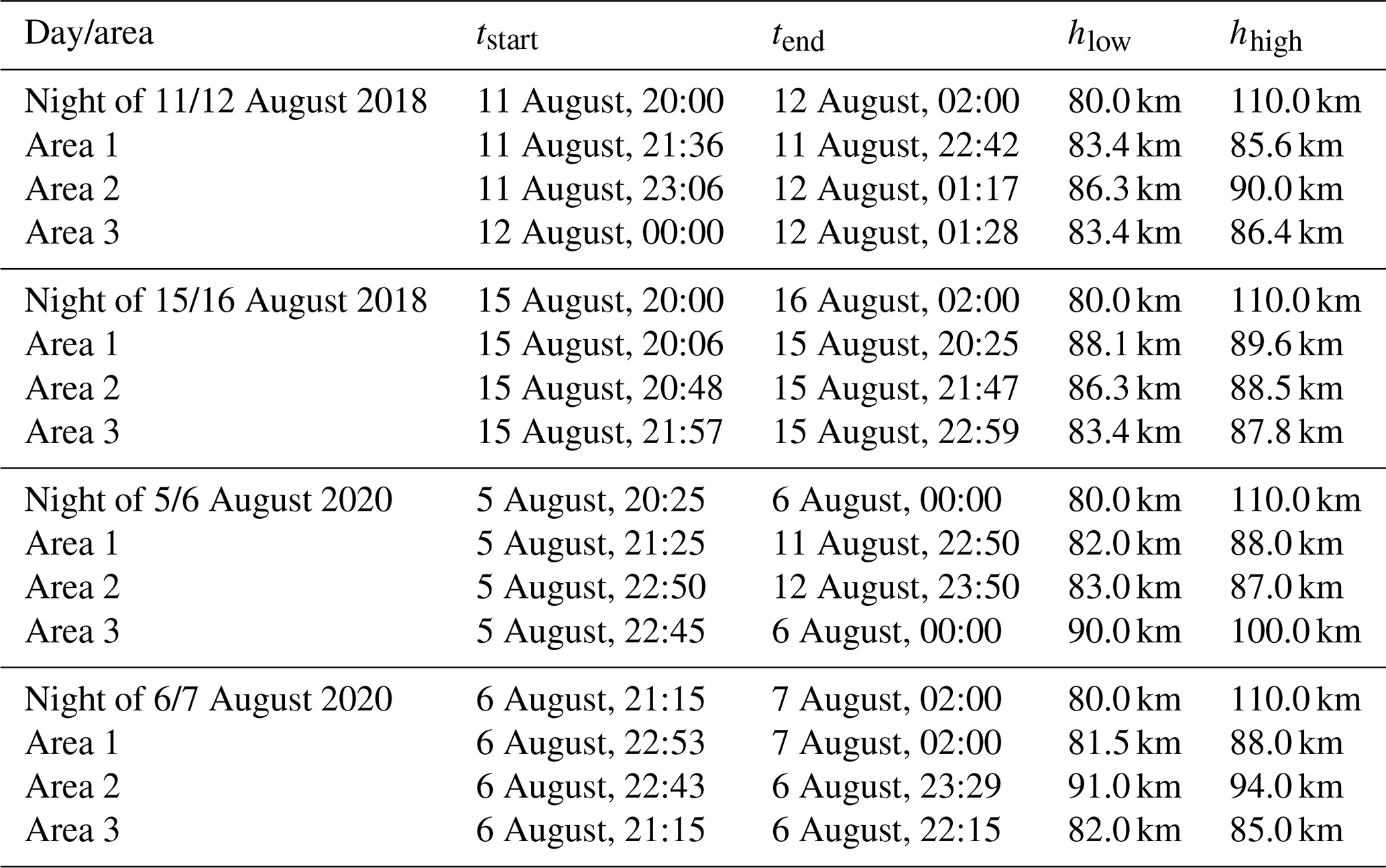
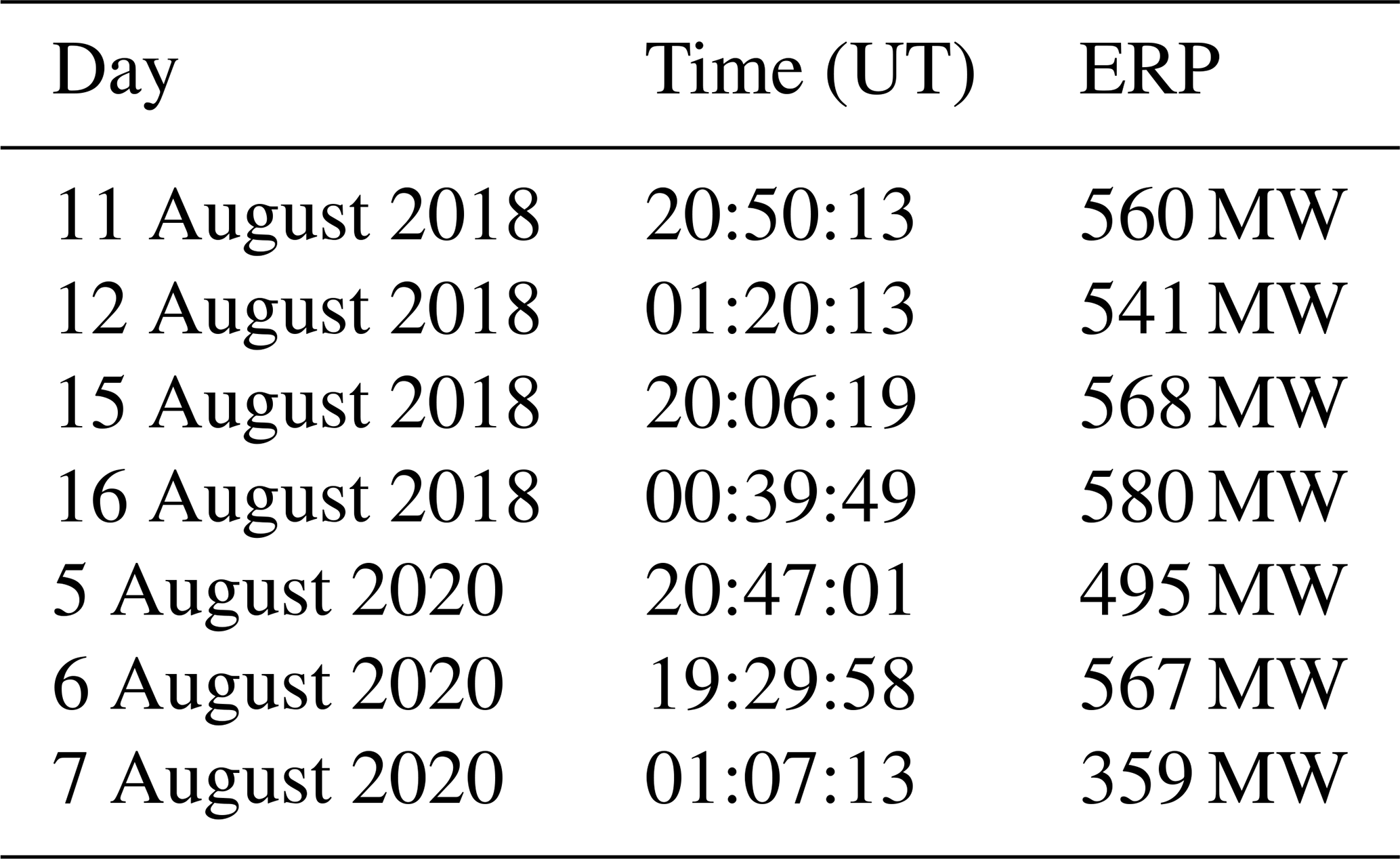
Table A2 Values of ERP given in the EISCAT heating facility logs from sample beam patterns for each of the measurements for reference. It seems that on 6 August 2020 at around 23:08:25 UT three transmitters changed phases such that the beam became broader, with about 360 MW X-mode and 17 MW O-mode, which remained so until the end, which is why we have 359 MW X-mode at 01:07:13 UT (7 of August).