Statistical distribution of mirror-mode-like structures in the magnetosheaths of unmagnetized planets – Part 2: Venus as observed by the Venus Express spacecraft

In this series of papers, we present statistical maps of mirror-mode-like (MM) structures in the magnetosheaths of Mars and Venus and calculate the probability of detecting them in spacecraft data. We aim to study and compare them with the same tools and a similar payload at both planets. We consider their dependence on extreme ultraviolet (EUV) solar flux levels (high and low).

The detection of these structures is done through magnetic-field-only criteria, and ambiguous determinations are checked further. In line with many previous studies at Earth, this technique has the advantage of using one instrument (a magnetometer) with good time resolution, facilitating comparisons between planetary and cometary environments.

Applied to the magnetometer data of the Venus Express (VEX) spacecraft from May 2006 to November 2014, we detect structures closely resembling MMs lasting in total more than 93 000 s, corresponding to about 0.6 % of VEX's total time spent in Venus's plasma environment. We calculate MM-like occurrences normalized to the spacecraft's residence time during the course of the mission. Detection probabilities are about 10 % at most for any given controlling parameter.

In general, MM-like structures appear in two main regions: one behind the shock and the other close to the induced magnetospheric boundary, as expected from theory. For solar maximum, the active region behind the bow shock is further inside the magnetosheath, near the solar minimum bow shock location. The ratios of the observations during solar minimum and maximum are slightly dependent on the depth $\mathrm{\Delta }B/B$ of the structures; deeper structures are more prevalent at solar maximum. A dependence on solar EUV (F10.7) flux is also present, where at higher F10.7 flux the events occur at higher values than the daily-average value of the flux. The main dependence of the MM-like structures is on the condition of the bow shock: for quasi-perpendicular conditions, the MM occurrence rate is higher than for quasi-parallel conditions. However, when the shock becomes “too perpendicular” the chance of observing MM-like structures reduces again.

Combining the plasma data from the Ion Mass Analyser (IMA on board Venus Express) with the magnetometer data shows that the instability criterion for MMs is reduced in the two main regions where the structures are measured, whereas it is still enhanced in the region between these two regions, implying that the generation of MMs is transferring energy from the particles to the field. With the addition of the Electron Spectrometer (ELS on board Venus Express) data, it is possible to show that there is an anti-phase between the magnetic field strength and the density for the MM-like structures.

This study is Part 2 of a series of papers on the magnetosheaths of Mars and Venus.

1 Introduction

Mirror modes (MMs) are ubiquitous structures in space plasmas, which consist of trains of magnetic depressions combined with plasma density enhancements in anti-phase. They are stationary in the plasma frame and convect with the plasma flow. Most often, these structures are found in planetary magnetosheaths, behind a quasi-perpendicular bow shock (BS). MMs have been found at Earth (e.g. Tsurutani et al., 1982; Baumjohann et al., 1999; Lucek et al., 1999a; Soucek et al., 2015), Venus (e.g. Bavassano Cattaneo et al., 1998; Volwerk et al., 2008b, c, 2016; Schmid et al., 2014), Mars (e.g. Bertucci et al., 2004; Espley et al., 2004; Simon Wedlund et al., 2022), Jupiter (e.g. Erdös and Balogh, 1996; Joy et al., 2006), Saturn (e.g. Bavassano Cattaneo et al., 1998) and comets (e.g. Mazelle et al., 1991; Glassmeier et al., 1993; Schmid et al., 2014; Volwerk et al., 2014).

1.1 MM instability and temperature anisotropy

MMs are created by a temperature anisotropy in the plasma, where the perpendicular temperature, T_⟂ (with respect to the magnetic field), is higher than the parallel temperature, T_‖. Hasegawa (1969) showed that for a bi-Maxwellian multi-component plasma the instability criterion is given by

$$\begin{array}{}\text{(1)}& \text{MMI}=\mathrm{1}+\sum _i{\mathit{\beta }}_{i⟂}\left(\mathrm{1}-{\displaystyle \frac{T_{i⟂}}{T_{i\Vert }}}\right)<\mathrm{0},\end{array}$$

where

$$\begin{array}{}\text{(2)}& {\mathit{\beta }}_{i,⟂}={\displaystyle \frac{n_i{k}_{\mathrm{B}}{T}_{i⟂}}{B^{\mathrm{2}}/\mathrm{2}{\mathit{\mu }}_{\mathrm{0}}}}\end{array}$$

is the perpendicular plasma beta of species i, the ratio of perpendicular (to the magnetic field) plasma pressure and the magnetic pressure. Here n_i is the density of species i, k_B is Boltzmann's constant, and μ₀ is the permeability of vacuum.

This temperature anisotropy can give rise to two different instabilities: the (Alfvén) ion cyclotron instability for low-β plasma and the mirror-mode instability for high-β plasma (Gary, 1992; Gary et al., 1993). In this paper, we will only consider the solar wind plasma and, therefore, only i=p (protons). Southwood and Kivelson (1993) rewrote the instability criterion, for protons p only, as R_SK>1, where

$$\begin{array}{}\text{(3)}& R_{\text{SK}}={\displaystyle \frac{T_{p,⟂}/T_{p,\Vert }}{\mathrm{1}+\mathrm{1}/{\mathit{\beta }}_{p,⟂}}},\end{array}$$

which is often used in papers lately (e.g. Wang et al., 2020), sometimes enhanced through a modified β^∗, which takes into account the ion-Larmor radius effects (Pokhotelov et al., 2004).

The increase in the perpendicular temperature or pressure can be created in various ways, which may be concurrent in the plasma: through pickup, where the newly created ion starts gyrating around the magnetic field; through perpendicular energization whilst crossing the quasi-perpendicular bow shock; and through slow changes in the magnitude of the magnetic field with conservation of the first adiabatic invariant. The first process will occur mainly in the solar wind interaction with the planetary exosphere (with the exception of Jupiter's magnetosphere and the Galilean moons, where the Jovian corotating magnetic field and magnetospheric plasma are taking the role of the solar wind) in the low-β plasma case, and generation of ion cyclotron waves will take place (Delva et al., 2008, 2009, 2011, 2015; Schmid et al., 2021). After crossing the quasi-perpendicular bow shock (where the interplanetary magnetic field (IMF) direction is near-perpendicular to the bow shock normal, with this angle ${\mathit{\theta }}_{\text{Bn}}>\mathrm{45}{}^{\circ }$), the anisotropy is increased, as is the plasma beta, and the MM instability will take over. The third process will occur mainly near the magnetic pileup boundary where the magnetic field gets compressed and slowly increases in strength whilst getting closer to Venus.

The temporal evolution of MMs, while they are convected with the plasma flow, has been discussed by Hasegawa and Tsurutani (2011). It was assumed that there is a Bohm-like diffusion (Bohm et al., 1949) taking place in the MM structures, where the higher frequencies of the structure diffuse faster than the lower ones; thereby, the MMs grow in size. This phenomenon was shown to occur at Venus and at comet 1P/Halley (Schmid et al., 2014).

The temperature anisotropy of the plasma is an important factor in the generation of MMs. Lately, the data of the Ion Mass Analyser (IMA) of the ASPERA-4 instrument (Barabash et al., 2007), as part of the Venus Express mission, have been re-evaluated and reprocessed by Bader et al. (2019), with the special focus of deducing the proton temperatures, T_‖ and T_⟂. This resulted in maps displaying, amongst others, the temperature anisotropy necessary for the MM instability criterion in Eq. (1). It also showed that mainly in the “near-subsolar magnetosheath” there was a high ratio of $T_{⟂}/T_{\Vert }\approx \mathrm{1.56}$, whereas in other regions this ratio was ∼1.

Rojas Mata et al. (2022) extended this study and also took into account the possible differences between solar minimum and maximum conditions. They found that T_‖ and T_⟂ are 20 % to 35 % lower during solar maximum as compared with solar minimum. However, the ratio $T_{⟂}/T_{\Vert }$ does not change, but the regions with a higher anisotropy are found further away from the bow shock during solar maximum conditions.

1.2 Earlier statistical study: Volwerk et al. (2016)

In an earlier study by Volwerk et al. (2016), MMs were studied for solar maximum conditions, using 1 Venus year (224 Earth days, from 1 November 2011 to 10 June 2012), and then the results were compared with the results of an earlier solar minimum study (224 Earth days, from 24 April to 31 December 2006; Volwerk et al., 2008c). As expected, the occurrence rate of MM-like¹ structures was maximum just behind the bow shock and close to the planet at the magnetic pileup boundary. Also, it was shown that the occurrence of MM-like structures was strongly dependent on the angle between the IMF and the bow shock normal, and they mainly occur for quasi-perpendicular shocks.

By comparing the two statistically obtained results, the following conclusions were drawn about the difference between solar minimum and maximum conditions:

1. The number of MM-like structures at solar maximum is slightly higher than at solar minimum by ∼14 %;

2. The observational rate for both solar conditions is the same because of the interplay of lower solar wind density and higher solar wind velocity during solar maximum than during solar minimum. One should keep in mind that cycle 24 is known to have a very weak solar maximum and thus may not be representative of more regular maxima;

3. The distribution of the number of MM-like structures as a function of the strength $\mathcal{B}=\mathrm{2}\mathrm{\Delta }B/B$ is exponential with approximately the same coefficient for both solar conditions for weak MM-like structures (i.e. ℬ≤1.2). There is a less steep exponential for strong MM-like structures (i.e. ℬ≥0.8) with significant differences in the exponential for solar minimum and maximum;

4. Freshly created MM-like structures behind the bow shock are on average stronger for solar minimum than for solar maximum;

5. For solar minimum, the general trend for MM-like structures is to decay; for solar maximum, MM-like structures first grow and then decay, between the bow shock and the terminator;

6. The estimated growth rates for the MM-like structures agree well with those found for the Earth's magnetosheath.

In these past studies the MM detection was performed with magnetometer data only. Subsequently, a coarse-grid determination of the temperature ratio $\mathcal{T}=T_{⟂}/T_{\Vert }$ by Bader et al. (2019) was used to check if the MM-like structures' observational rate distribution agreed with the temperature anisotropy distribution in Venus's magnetosheath. It was shown that indeed, where 𝒯 is large, the largest observational rates of MM-like structures was found.

In this paper we make a statistical study of the Venus Express (VEX; Svedhem et al., 2007) mission magnetometer (VEXMAG; Zhang et al., 2006) data over the full mission from May 2006 to November 2014. Additional information is obtained through the plasma data from the ASPERA-4 instrument (Barabash et al., 2007) for both the ions and the electrons. This new and larger study is performed together with a companion paper by Simon Wedlund et al. (2023a, Part 1) which uses the same detection criteria for MM-like structures over the full MAVEN mission data at Mars, making it possible to directly compare, for the first time, the distribution of MM-like structures at the two planets.

2 Detecting mirror-mode-like structures in spacecraft data

2.1 Instrumentation

VEX was brought into a polar orbit around Venus in 2005 with an elliptical orbit and periapsis at ∼300 km from the surface, which means the spacecraft entered well into the induced magnetosphere. The VEXMAG data used here have a sampling rate of 1 Hz but are also available at 32 Hz (and for short intervals a sampling rate of 128 Hz exists). However, as the MM structures have a period of $\mathrm{4}\le T_{\text{mm}}\le \mathrm{15}$ s (Volwerk et al., 2008b, c, 2016), the 1 Hz data downsampling is sufficient. Unfortunately, the data from the Ion Mass Analyser (IMA on board VEX) of the ASPERA-4 instrument (Barabash et al., 2007) only has a resolution of 192 s for ions, which means that these data can only give us an indication of the overall plasma conditions (see, for example, Bader et al., 2019; Rojas Mata et al., 2022).

In contrast, the Electron Spectrometer (ELS) of ASPERA-4 has a cadence of 4 s at full energy resolution (1 eV–20 keV) with regular switches to 1 s resolution at limited energy resolution (10–130 eV), which would be sufficient to analyse the larger MMs for an anti-phase between magnetic field strength and electron density. Lately, Fränz et al. (2017) calculated the electron densities for the whole Venus Express mission (where feasible), where they only used omnidirectional spectra from ELS to determine the electron densities and temperatures.

In this paper the full dataset over the VEX mission period is used, from May 2006 to November 2014, which contains both a solar minimum and solar maximum period as is shown in Fig. 1 (see also Delva et al., 2015; Volwerk et al., 2016). In this way there can be a comparison between the probability and location of MM-like structures in either solar activity period.

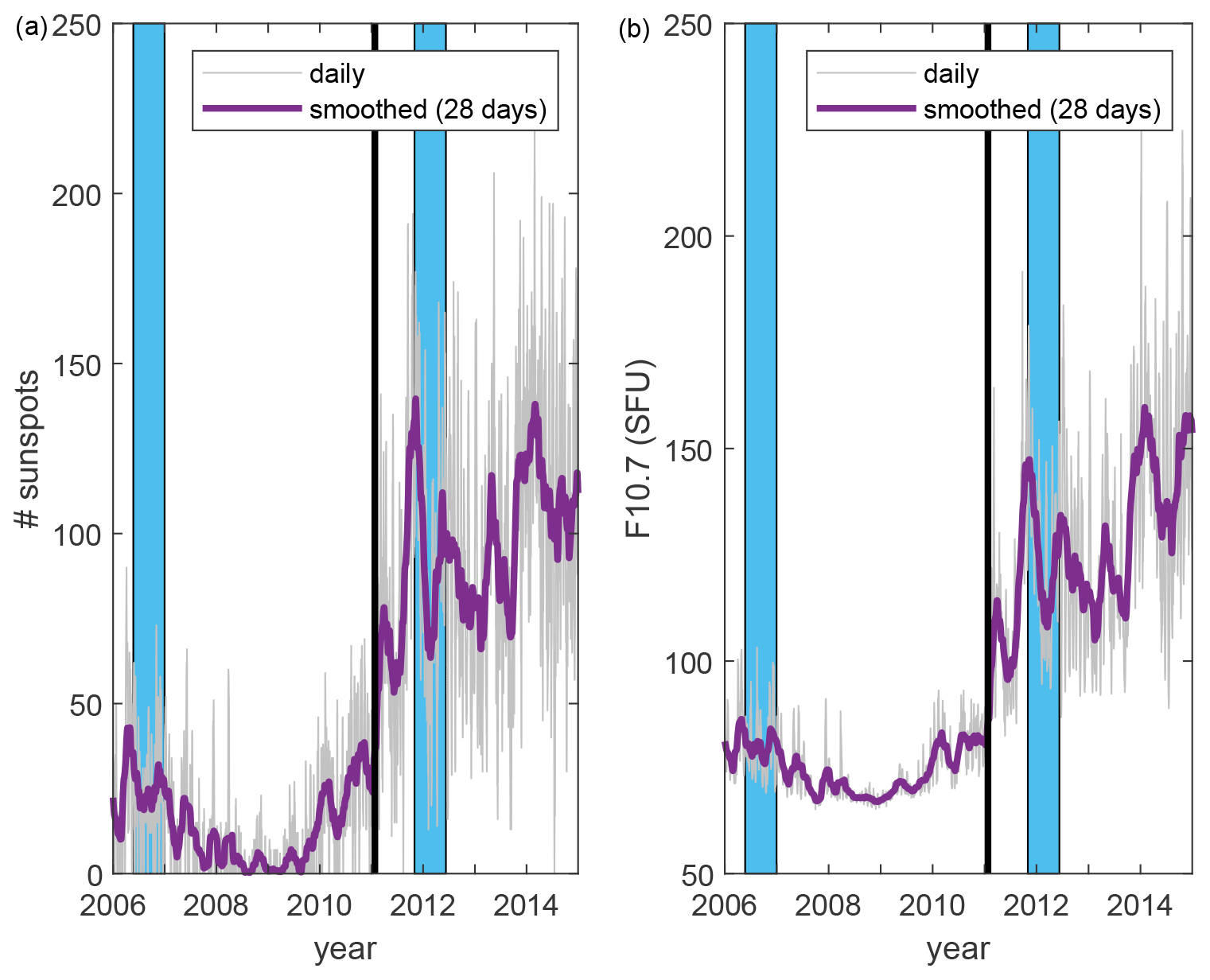
Figure 1 The daily (grey) numbers of sunspots (a) and F10.7 flux (b) over the duration of the VEX mission (2006–2014) and the smoothed (over 28 d) numbers (purple). The vertical line at 25 January 2011 is marking the (slightly arbitrary) boundary between the solar minimum and solar maximum periods, split at no. of sunspots = 50 or F10.7 = 100 SFU (solar flux units). The two blue boxes show the intervals discussed in Volwerk et al. (2016).

2.2 Detection method

2.2.1 B-field-only criteria

In order to detect the MM-like structures in the VEXMAG data, we use the method introduced by Simon Wedlund et al. (2022), which is slightly different but more accurate than that used by Volwerk et al. (2008b). Because of the lack of high-time-resolution ion data and the limited plasma (electron and ion) data availability, the detection method is based on magnetic field measurements only. We use the same criteria as in Table 1 of the companion paper Part 1, which are based on several previous studies including Lucek et al. (1999a, b) and Volwerk et al. (2008b) and expanded on by Simon Wedlund et al. (2022).

1. The magnetic field data, B, are low-pass filtered with a 2 min wide Butterworth filter to determine the background field B_bg, with $\left|{\mathbf{B}}_{\text{bg}}\right|>\mathrm{5}$ nT to isolate magnetosheath conditions from average solar wind values;

2. From the data and the background field, we calculate $\mathrm{\Delta }\left|\mathbf{B}\right|/\left|{\mathbf{B}}_{\text{bg}}\right|=\left(\right|\mathbf{B}|-|{\mathbf{B}}_{\text{bg}}\left|\right)/\left|{\mathbf{B}}_{\text{bg}}\right|$, where a threshold is set to $\mathrm{\Delta }\left|\mathbf{B}\right|/\left|{\mathbf{B}}_{\text{bg}}\right|\ge \mathrm{0.15}$ (compressibility of the structure);²

3. Then we apply a minimum variance analysis (MVA; Sonnerup and Scheible, 1998) on 15 s wide sliding windows with a 1 s shift, to obtain the directions of the minimum and maximum variations. A requirement on the maximum, minimum and intermediate eigenvalues is set to ${\mathit{\lambda }}_{\text{max}}/{\mathit{\lambda }}_{\text{int}}\ge \mathrm{3}$ and ${\mathit{\lambda }}_{\text{int}}/{\mathit{\lambda }}_{\text{min}}\le \mathrm{8}$;

4. The angles between the minimum/maximum variation direction and the background magnetic field should be: ${\mathrm{\Phi }}_{\text{minV}}\ge \mathrm{70}{}^{\circ }$ and ${\mathrm{\Theta }}_{\text{maxV}}\le \mathrm{20}{}^{\circ }$;

5. The azimuth, $\text{az}=\arctan (B_y/B_z)$, and elevation, $\text{el}=\arctan (B_z/\sqrt{B_x^{\mathrm{2}}+B_y^{\mathrm{2}}})$, of the magnetic field are calculated, and for MM-like structures it is expected that the rotation of the magnetic field over the structure is $\mathrm{\Delta }(\text{az},\text{el})\le \mathrm{10}{}^{\circ }$.

The reasons of these choices above are explained in more detail in Part 1, to which the reader is referred.

2.2.2 Removal of false positive detections

In order to find when the spacecraft is in Venus's magnetosheath, the database of calculated bow shock crossings based on the models by Zhang et al. (2008) and Russell et al. (1988) was evaluated. There are more recent, more advanced, models for the bow shock, e.g. Martinecz et al. (2009), which was further developed by Chai et al. (2014). However, because of the relatively low variability of the Venus bow shock position (Martinecz et al., 2009; Chai et al., 2014, less than ±0.2R_V), we expect that a simple margin on the crossing times of ∼30 min, which corresponds to 14 400 km or 2.3R_V (with R_V=6051.8 km, Venus's radius), 10 times the variability, ensures that we capture the true bow shock in the data; there is no use in including these models.

We should note that around the bow shock there are other kinds of structures which have similar characteristics in polarization and compression as the MMs that we are looking for. These waves are also linked to pickup ion processes, in the case of the quasi-parallel shock. Consequently, looking at the magnetic field only, strong fluctuations ($\mathrm{\Delta }\left|\mathbf{B}\right|/B_{\text{bg}}\ge \mathrm{0.1}$) may appear, which are not sinusoidal and have a quasi-linear polarization, without these structures necessarily being MMs. Most of the time, magnetic field intensity and plasma density will typically be in phase, as opposed to the expected MM anti-phase behaviour (Hasegawa, 1969). However, this information is sometimes neither available at the desired high time resolution (as in our case with VEX data) nor practical to derive as in large statistical surveys.

As in Part 1, two strategies can be made in order to exclude non-MM signatures: (1) making sure that the magnetic field across the structure's region does not rotate more than 10–20^∘, as theoretically predicted for MMs (Treumann et al., 2004) and in agreement with past observations (Tsurutani et al., 2011), and (2) restricting the detections to magnetosheath conditions only and excluding the region around the bow shock to avoid these foreshock transients.

Strategy (1) constrains the detected structures to behaviours more reminiscent of MMs: we apply criterion 5 listed in Sect. 2.2, which ensures that the magnetic field does not rotate significantly across the structure. From the magnetic field vector, the magnetic azimuth and elevation angles are defined as

$$\begin{array}{}\text{(4)}& \text{az}=\arctan (B_y/B_x)\end{array}$$

and

$$\begin{array}{}\text{(5)}& \text{el}=\arctan \left(B_z/\sqrt{B_x^{\mathrm{2}}+B_y^{\mathrm{2}}}\right).\end{array}$$

First, we define detection periods, which contain structures detected within a maximum of 30 s between one another and ignore isolated singular events; two separate regions are thus more than 30 s apart. This particular value of 30 s was chosen empirically as double the length of the longest MM structures found at Mars or Venus (see, for example, Simon Wedlund et al., 2022; Volwerk et al., 2008c, 2016); moreover, this ensures that rotations could be calculated for trains of MM-like structures for which the 2 min windowed background magnetic field values would be representative. We then estimate how much azimuth and elevation angles fluctuate at the detected position of the candidate structure by calculating their running standard deviation 〈σ(az,el)〉 over a 2 min sliding interval, keeping only those structures where 〈σ(az,el)〉 is less than 10^∘ for each angle (Simon Wedlund et al., 2022,  CSW). This analysis of the data will be called the CSW method.

Complementarily, strategy (2) makes use of the position of the bow shock crossing in the spacecraft data and ignores the detected structures in a range of radial distances around it (or equivalently, in a range of durations around the time of the crossing).

For Mars, the automatic bow shock predictor–corrector algorithm based on magnetic-field-only measurements was used, explained in Simon Wedlund et al. (2022). This analysis has not (yet) been done for Venus; thus, this product does not exist. Therefore, only the first strategy has been applied in this paper.

2.2.3 Examples

Figure 2 shows a 3 min interval of VEXMAG data on 5 May 2006, where VEX is in Venus's magnetosheath (see also Volwerk et al., 2008c, Fig. 1), where the selection criteria by Volwerk et al. (2008b, grey) and by Simon Wedlund et al. (2022, green) are compared. It is clear that in the magnetosheath, around 01:17 UT, both methods find the same MM-like structures. The old criteria capture events in the shock and just behind it which are obvious false positives, while they are filtered out in the new method. Moreover, the reason we also remove the events around 01:16 UT is that the eigenvalue ratios (and thus the more stringent linear polarization criteria) are not fulfilled any more in the new method. Because of the additional restrictions, the CSW method identifies fewer but more fully formed MM-like structures.

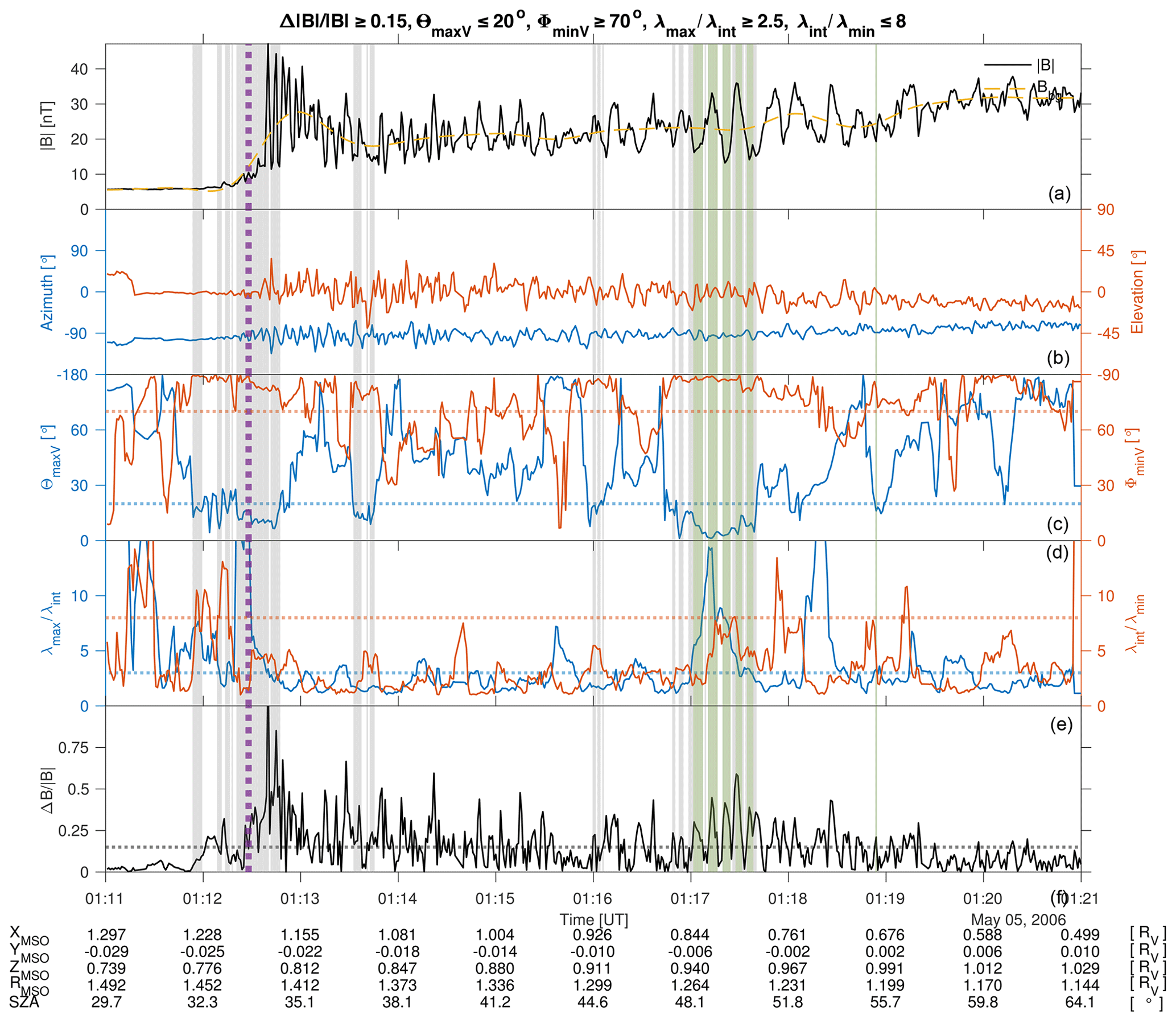
Figure 2 Ten minutes on 5 May 2006 when VEX entered through the bow shock into the magnetosheath. Shown are (a) the total magnetic field; (b) the azimuth and elevation of the magnetic field; (c) the angles of the minimum and maximum variation direction with the background magnetic field; (d) the ratios of the eigenvalues; and (e) the $\mathrm{\Delta }B/B$. The grey shading shows the events found with the criteria in Volwerk et al. (2008b), and the green shading shows those found with the criteria in Simon Wedlund et al. (2022) (with the green shading overlapping the grey shading). The vertical, dotted purple line is the model location of the nominal bow shock. Note that for this event there are no electron data available.

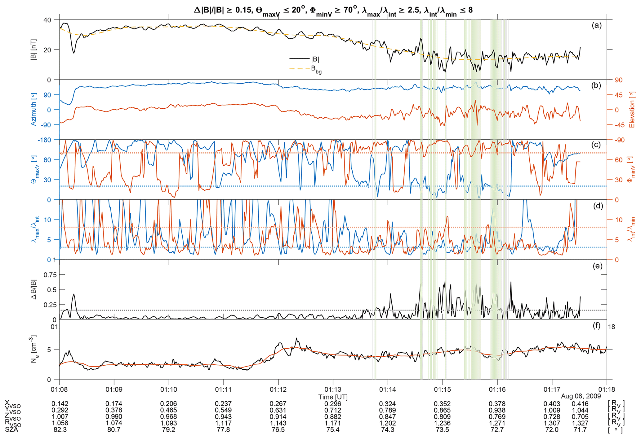
In Fig. 3 the inbound part of a solar maximum orbit of VEX is shown, where there are some determinations of MM-like structures close to the BS and further inside the magnetosheath. Here we notice that both methods basically find the same events. There are no rejections using the CSW method.

Figure 3 Ten minutes on 8 August 2009 when VEX returned from the pericentre through the magnetic pileup region close to Venus. Same format as Fig. 2. For this event, there are electron data from ASPERA-4 ELS in the bottom panel.

2.3 Mapping technique

Following the mapping technique of Part 1, the results are shown on a grid in cylindrical coordinates based on the VSO coordinate system,³ i.e. X_VSO and $R_{\text{VSO}}=\sqrt{Y_{\text{VSO}}^{\mathrm{2}}+Z_{\text{VSO}}^{\mathrm{2}}}$ with a size of 0.1×0.1R_V. For each grid cell, the total number of seconds for which the MM criteria are fulfilled, ΔT^struct, is calculated as well as the total residence time of VEX in that box, ΔT^sc. Both determinations are done for solar minimum and solar maximum. The probability of MM-like structures is then simply calculated from the ratio of the two:

$$\begin{array}{}\text{(6)}& \mathcal{P}={\displaystyle \frac{\mathrm{\Delta }{T}^{\text{struct}}}{\mathrm{\Delta }{T}^{\text{sc}}}}.\end{array}$$

We only consider grid cells where the spacecraft stayed at least 30 min in cumulated time, to ensure good statistics throughout.

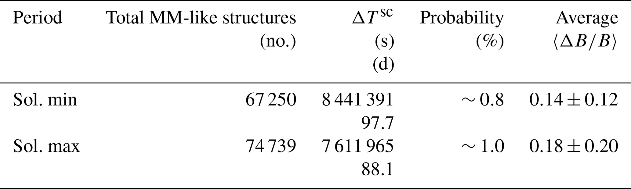
A first quick result can be obtained by looking at the total duration of MM-like structures spanning years 2004–2016 of VEXMAG data, as shown in Table 1. The total residence time shows that VEX stayed longer in the magnetosheath at solar minimum than at solar maximum. This is caused by the asymmetric division between solar minimum and maximum of the VEX mission (see Fig. 1) and is influenced by a change in attitude of the orbit over the duration of the mission, where the semi-major axis slowly rotated further southward and in the late stage of the mission back northward again. Nevertheless, more events are found, and the total observational rate is ∼50 % higher during solar maximum. Note that, although these are both multiple years of orbits, the time spent in the magnetosheath is actually rather short, 185.8 d out of 3195, because of the highly elliptical orbit with a periapsis and apoapsis of 250 km (1.04R_V) and 66 000 km (11.90R_V), respectively, whereas the magnetosheath spans typical radial distances of 1.1 to 1.5–3R_V.

Table 1 Total number of MM-like structures in the VEXMAG dataset (equivalent to a duration (in s) because of the magnetometer resolution of 1 s) and residence times in the magnetosheath, probability 𝒫 of observing mirror-mode structures during that time, and averaged MM depth $\langle \mathrm{\Delta }B/B\rangle$ for solar minimum and maximum conditions.

In Figs. 7 and 8 (left panels) the total residence time of the spacecraft in 0.1×0.1R_V cells is shown for solar minimum and maximum. It shows that there is a slight difference of total residence times in, for example, the polar region (at X_VSO=0), where VEX spent relatively less time during the solar maximum interval.

2.4 Calculating MM-like observational probability

The overall numbers and probabilities only give a rough indication that MM-like structures are more prone to be excited during solar maximum as compared to solar minimum. The interesting part is when the probability per 0.1×0.1R_V cell is examined.

Figures 7 and 8 show the statistical results of our search for solar minimum and maximum, respectively. The left panels show the total residence time ΔT^sc of VEX in each grid cell. The middle panel shows the probability of MM-like structures per cell calculated with Eq. (6). The right panel shows the mean $\langle \mathrm{\Delta }B/B\rangle$ in each grid cell, limited by the restriction that $\langle \mathrm{\Delta }B/B_{\text{bg}}\rangle \ge \mathrm{0.15}$.

There are clearly two regions on the dayside where the MM-like structures are most prevalent: for solar minimum right behind the BS and close to the ionopause and for solar maximum also behind the bow shock but slightly deeper inside the magnetosheath, as well as again at the magnetopause/ionopause. In a marginal way, there is also a third area behind the planet, around $(X,R)=(-\mathrm{2},\mathrm{0})R_{\mathrm{V}}$, where MM-like structures seem to be present for solar maximum, which is not so prominent at solar minimum. One may assume, in a first approximation, that the structures are observed where they are generated, that is, that the creation of the first two regions is caused by two anisotropic energization mechanisms of the ions: close to the bow shock the perpendicular temperature is enhanced by preferential heating along the perpendicular direction to the magnetic field of ions crossing the quasi-perpendicular BS; close to the magnetopause/ionopause the perpendicular temperature is enhanced by the magnetic pileup in front of the planet and the conservation of the first adiabatic invariant.

2.5 Controlling parameters

The presence of MM-like structures in Venus's magnetosheath is first of all dependent on the type of bow shock. A quasi-perpendicular bow shock has its normal nearly perpendicular to the impinging IMF. In this case the picked-up protons in the solar wind are energized mainly in the direction perpendicular to the magnetic field. This increases the $T_{⟂}/T_{\Vert }$ term in the instability criterion, Eq. (1); thus, MM-like structures are expected to be generated. However, this criterion is not a sufficient condition, as was shown in the data from the Solar Orbiter flyby of Venus, where behind a near-perpendicular bow shock ion cyclotron waves (ICWs) were generated (Volwerk et al., 2021) instead of MM-like structures. This was caused by a low plasma beta (β≈1.3) behind the bow shock, in agreement with Gary et al. (1993), who showed that, for low plasma beta, the ratio $T_{⟂}/T_{\Vert }$ must be ∼15 % larger for MM generation than for ICW generation.

Behind a quasi-parallel bow shock, the generation of MM-like structures is not expected to be significant due to the lack of perpendicular energization of the protons, which was shown by Volwerk et al. (2008c). In this condition, pickup ion effects alone may lead to temperature anisotropies able to generate MMs (Gary, 1992).

Venus's orbit has an eccentricity of ϵ≈0.0068, which means that, unlike Mars with an eccentricity of ϵ≈0.0934, seasonal effects are not expected. However, the average bow shock location for solar minimum and maximum is significantly different. For example, the terminator distance is R_{t, min}≈2.14R_V (Zhang et al., 2008) and R_{t, max}≈2.40R_V (Russell et al., 1988): for solar maximum conditions, the bow shock significantly expands in the solar wind and inflates by more than 10 %. The difference between the two solar activities is clearly seen through the further distance into the magnetosheath of the MM probability peak for solar maximum.

It should be noted, however, that the maximum of solar cycle 24 was (much) weaker then previous solar maxima (see, for example,  McComas et al., 2013), which means that the solar wind conditions may not be representative of a regular solar maximum.

3 Results

3.1 Overview of the full dataset

In Fig. 4 we show the probability distribution function (PDF) of all variables necessary in the selection criteria listed in Sect. 2.2 for the whole mission. The maxima of the PDFs have been indicated by a grey bar in the panels. These PDFs need to be checked against the selection criteria. Panels (b) through (f) of the histograms show only that the bulk of MM-like events peak at around 7 nT of B field (nominal magnetosheath values), at $\mathrm{\Delta }B/B$ of 0.17 (threshold being 0.15), with a perpendicular direction to the minimum variance direction and a very broad, flat distribution of maximum variance directions between 10 and 20^∘ (peak at 16^∘).

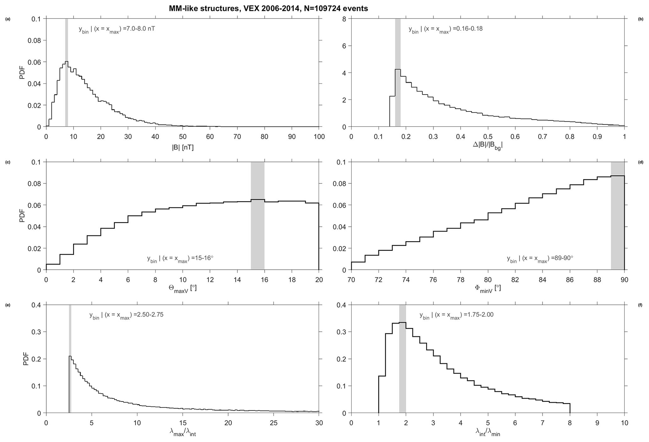
Figure 4 Probability distribution functions (PDFs) of selection criteria for MM-like structures in the VEX magnetometer data for the whole mission. (a) Total magnetic field intensity $\left|\mathbf{B}\right|$, in bins of 1 nT. (b) Magnetic field fluctuations $\mathrm{\Delta }\left|\mathbf{B}\right|/B_{\text{bg}}$, in bins of 0.02. (c and d) Angles between average magnetic field direction and maximum (minimum) variance direction Θ_maxV (Φ_minV), in bins of 1^∘. (e and f) Ratios of maximum to intermediate ${\mathit{\lambda }}_{\text{max}}/{\mathit{\lambda }}_{\text{int}}$ (intermediate to minimum, ${\mathit{\lambda }}_{\text{int}}/{\mathit{\lambda }}_{\text{min}}$) eigenvalues, in bins of 0.25. The position of the maximum of the PDF and its typical bin is marked by a grey zone. All bins are uniformly distributed.

Indeed, putting together all criteria, we obtain the official number of MM-like structures in Venus's magnetosheath. In Fig. 5 we show the daily occurrence rate of these structures over the whole VEX mission, with a 7 d running average overlaid in red. The average number of observed events per day is $\langle N\rangle =\mathrm{26}\pm \mathrm{23}$. However, as mentioned earlier, VEX only spends 185.8 d out of 3195 d in the magnetosheath, i.e. ∼6 % of the spacecraft orbiting time. Assuming on average a mirror-mode structure to last 10 s, we end up with about 26 mirror-mode structures observable per day. This means that to obtain the total number of events per day, we have to correct this by multiplying this number by a factor of $\mathrm{100}/\mathrm{6}$, which leads to 〈N_corr〉≈430 one-second events per day.

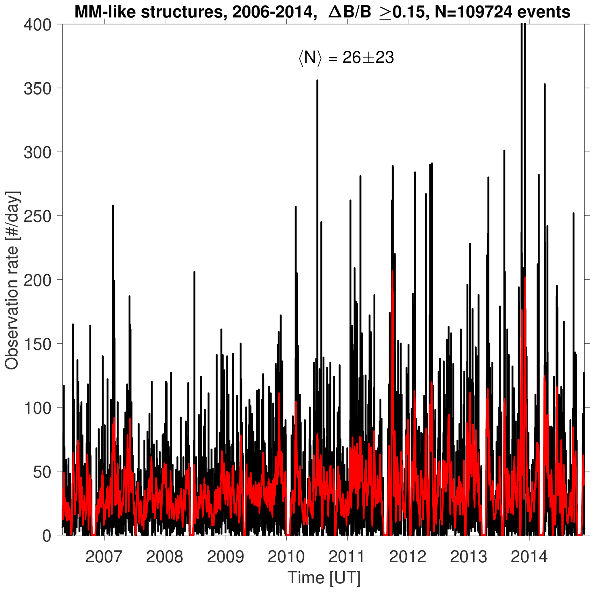
Figure 5 Daily observation rate of MM-like structures as observed by the VEX magnetometer for the whole mission, using the selection criteria mentioned in Sect. 2.2. The red line corresponds to the running mean of the black curve over 7 d. 〈N〉 is the median of the signal in black, with its corresponding standard deviation.

Figures 6–8 show the overall results of our analysis, for the whole dataset, and for solar minimum and maximum conditions, respectively. Displayed are the residence time of VEX around Venus, the probability 𝒫 to find MM-like structures in the X–R plane and the average depth of $\mathrm{\Delta }B/B$ in each grid cell. Figure 9 displays the absolute difference of detection probability between high solar activity and low solar activity.

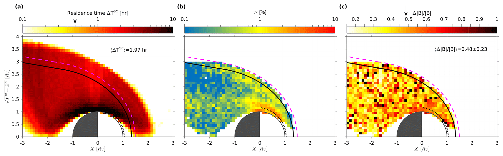
Figure 6 Full dataset. (a) The total residence time of Venus Express in the X–R plane. The thick black line is the bow shock location as determined by Zhang et al. (2008) for solar minimum. The dotted line is the magnetopause/ionopause location. (b) The dashed magenta line shows the location of the solar maximum bow shock. The probability of MM-like structures in the X–R plane is shown. There are two clear regions of increased 𝒫, just behind the bow shock and close to the magnetopause/ionopause. (c) The average depth of the mirror modes in each grid cell, limited by $\mathrm{\Delta }B/B\ge \mathrm{0.15}$.

Figure 7 Solar minimum; same format as Fig. 6.

Figure 8 Solar maximum; same format as Fig. 6.

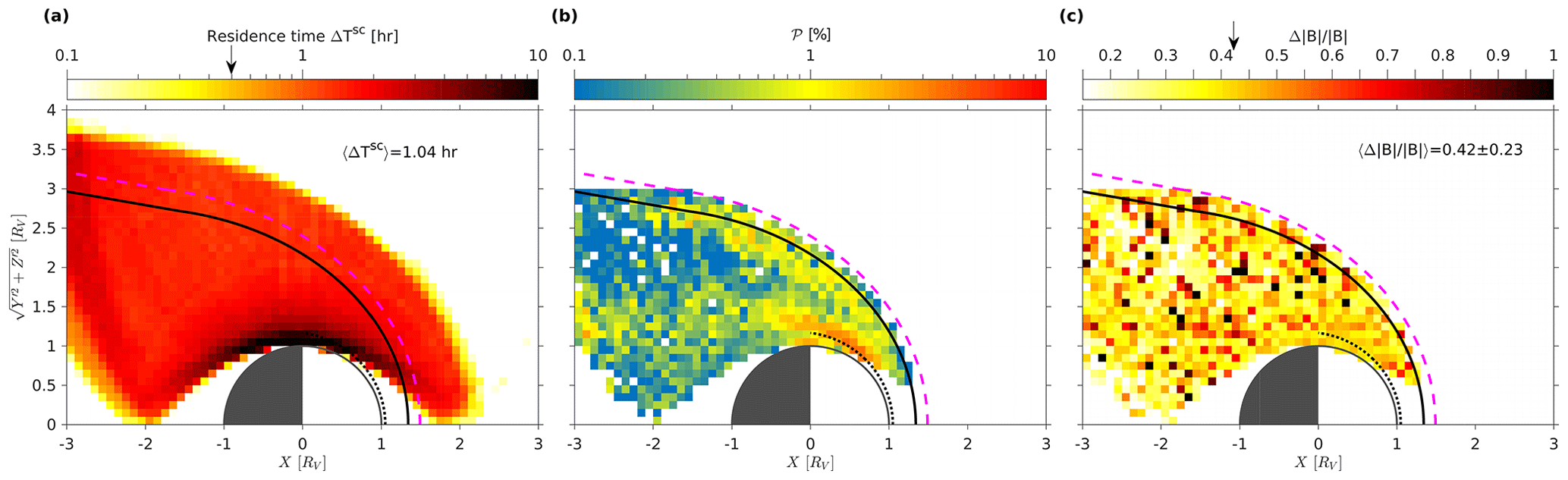
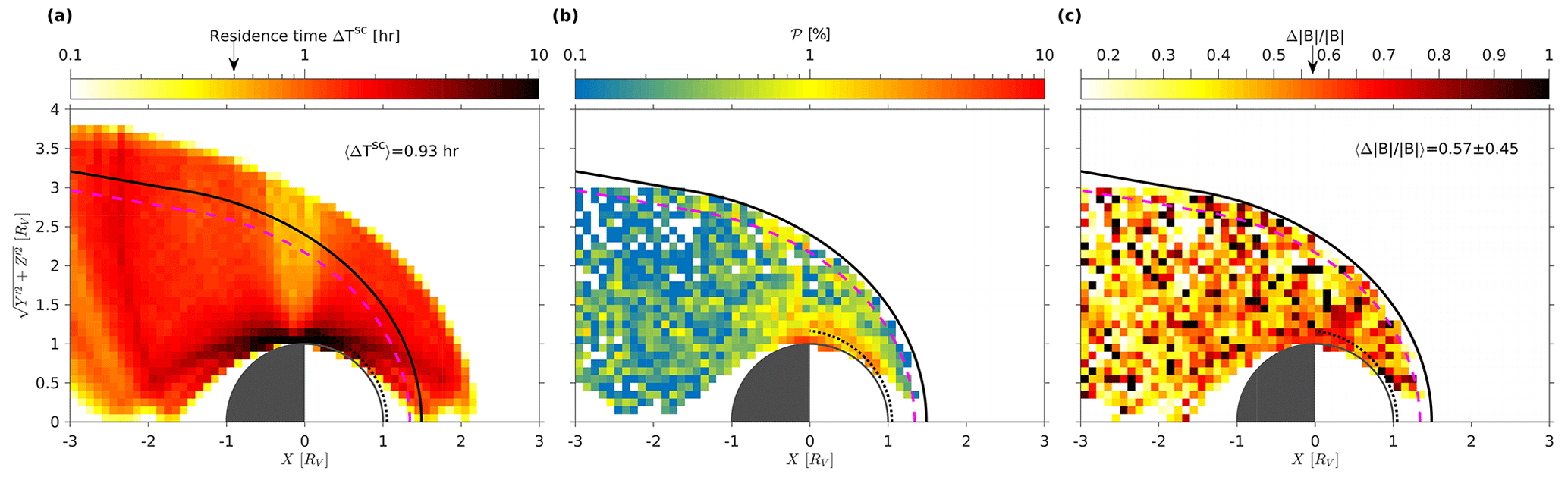
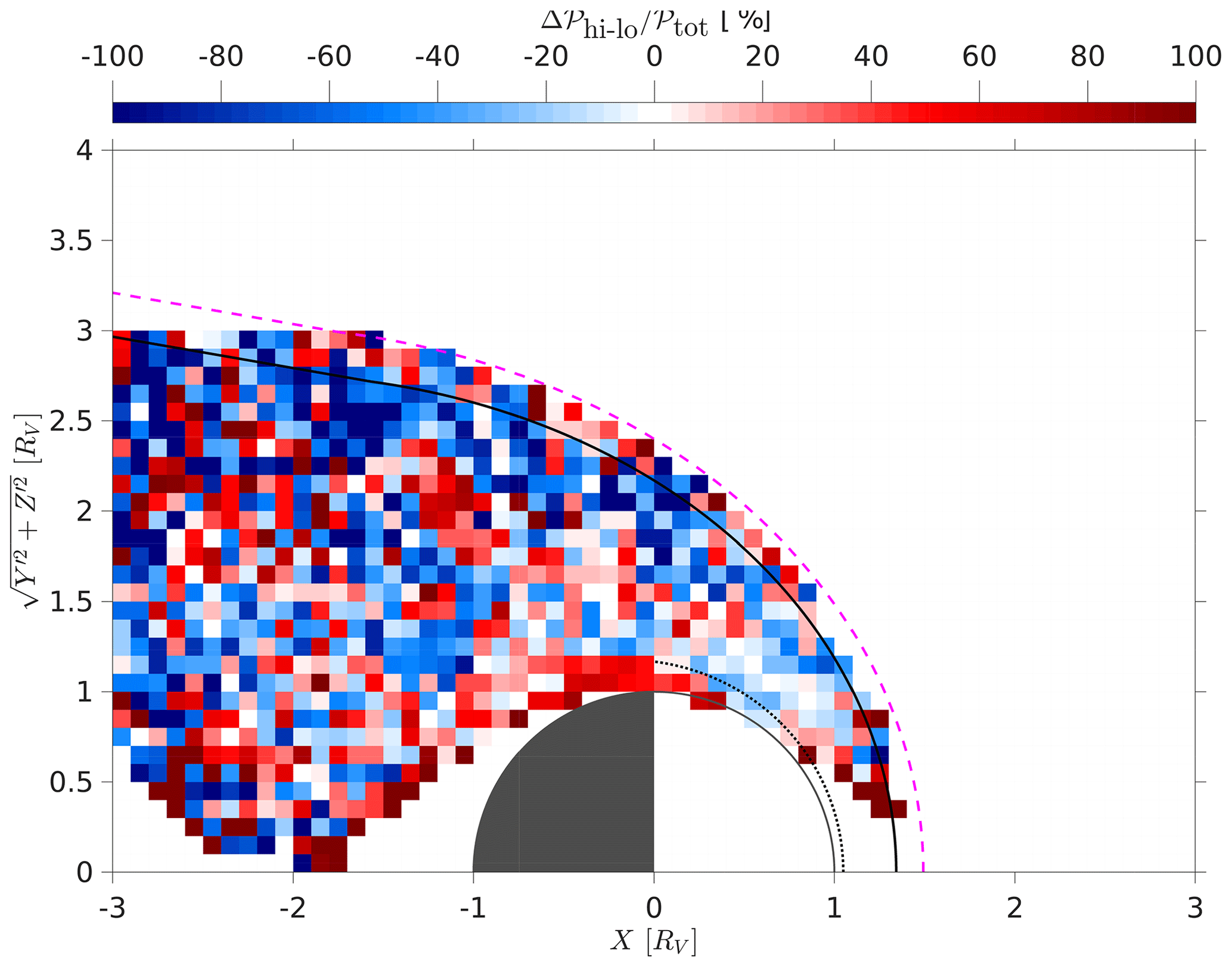
Figure 9 The difference between solar maximum and minimum in probabilities, calculated through $\left({\mathcal{P}}_{\text{hi}}-{\mathcal{P}}_{\text{lo}}\right)/\left({\mathcal{P}}_{\text{hi}}+{\mathcal{P}}_{\text{lo}}\right)$, with the red hues showing where the solar maximum conditions are dominating in that box and with the blue hues showing where solar minimum conditions are dominant.

The probability of MM-like structures for solar minimum and maximum, respectively, for the cleaned dataset, i.e. with requirements 1–5 from Sect. 2.2 applied, is calculated. As mentioned earlier, there seem to be two regions in which this rate is greatly enhanced compared to the rest of Venus's surroundings: just behind the bow shock and around the ionopause. Similarly, Figs. 7 and 8 (right panels) show the average depth of the observed MM-like structures in each bin. As shown in Table 1, the average values for $\langle \mathrm{\Delta }B/B\rangle$ are rather small for this dataset; however, the full distribution of $\mathrm{\Delta }B/B$ is shown in Fig. 10.

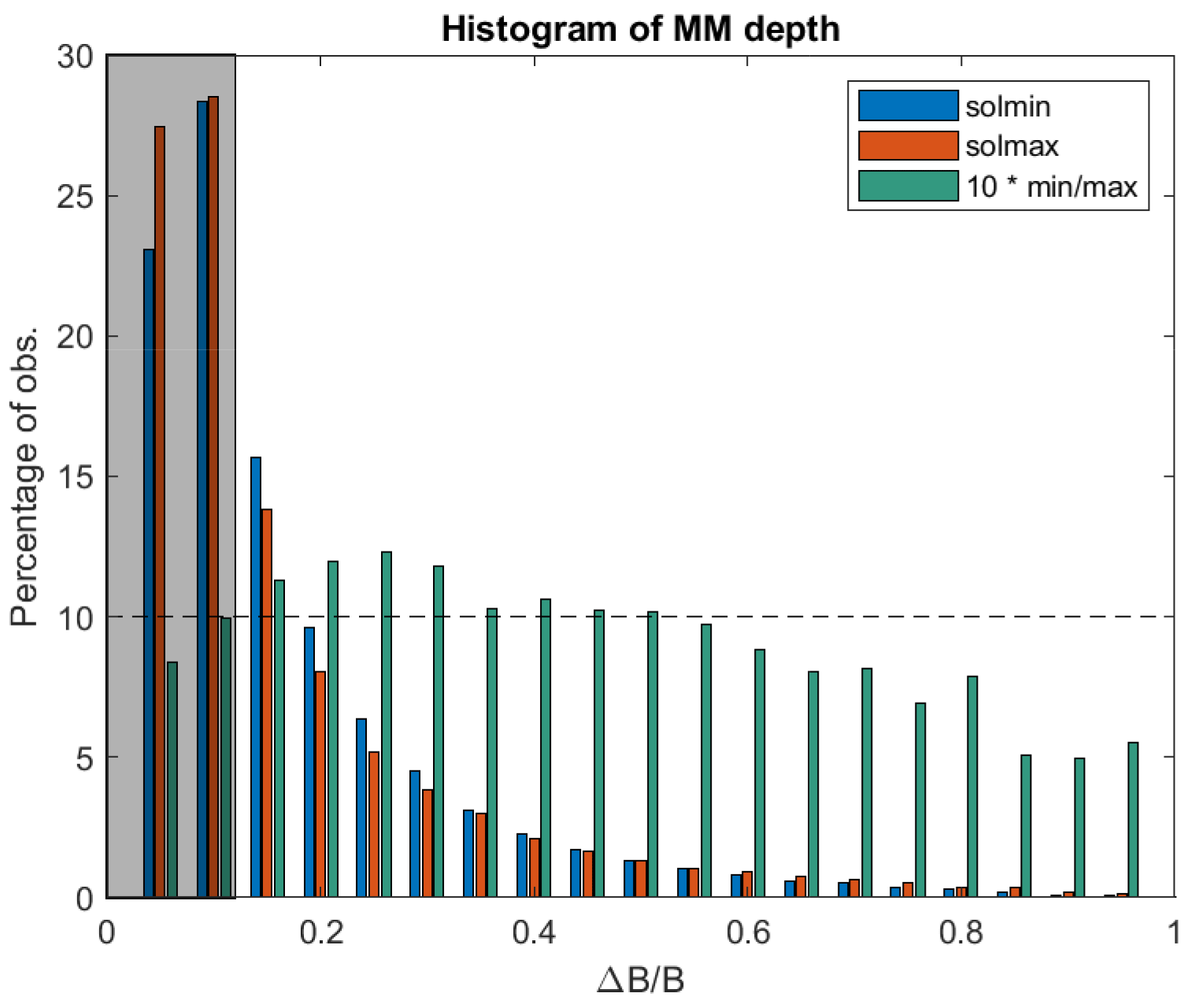
Figure 10 Histograms of the distribution of the depth $\mathrm{\Delta }B/B$ of the MM-like structures for solar minimum (blue) and maximum (red) and the ratio between the two (green = blue/red, multiplied by 10 for visibility). The grey shaded region shows the structures with $\mathrm{\Delta }B/B<\mathrm{0.15}$ that are not taken into account in the analysis in this paper.

First, we look at the depth of the MM-like structures. Figure 10 shows the distribution of the depth $\mathrm{\Delta }B/B$ of the MM-like structures, where the majority of the MM-like structures fall into the greyed-out category $\mathrm{0.05}\le \mathrm{\Delta }B/B\le \mathrm{0.15}$, which are not taken into account in the analysis as per the selection criteria.

Both distributions are very similar percentage-wise, indicating that solar activity has little influence on the depth. However, one can discern a dichotomy in the percentages between solar minimum and maximum. The green bars, describing the ratio of the percentages of solar minimum and maximum (𝒢 = blue/red, multiplied by 10 here for visibility) show that up until $\mathrm{\Delta }B/B=\mathrm{0.5}$ there is a higher percentage for solar minimum, 𝒢>1, and after that for solar maximum, 𝒢<1. It was shown above that the location of the MM-like structures is different as well as the total amount of MM-like structures measured: 38 901 and 64 883, respectively (see Table 1). Specifically, very deep events, $\mathrm{\Delta }B/B\ge \mathrm{0.75}$, are ∼5 times more abundant at solar maximum as compared to solar minimum, with 1973 and 357 events, respectively.

3.2 Dependence on solar activity

It was shown above, in Figs. 6–9, that the main differences in the probability of MM-like structures for solar minimum and maximum are as follows: (1) the total number of events measured and (2) the location within the magnetosheath where they were observed. As previously pointed out, no seasonal variations in the probability are expected. However, there can be other effects that can have an influence on the probability of MM-like structures.

As the MM-like structures behind the BS are mainly generated by freshly created pickup ions, re-energized by their crossing of the bow shock, it stands to reason that the solar extreme ultraviolet (EUV) flux plays a role, as photo-ionization is the main source for these particles. Indeed, it was shown by Delva et al. (2015) that the higher number of observed proton cyclotron waves for solar maximum, as compared to minimum, was caused by the higher EUV flux, supplying a greater number of newborn protons from Venus's exosphere.

The split between solar minimum and maximum based on sunspots is rather arbitrary, and a more sophisticated method can be used to study the influence of solar activity through the daily F10.7 flux. As can be seen in Fig. 1, however, the divide assumed in this paper splits the periods well with number of sunspots ≶50 or F10.7≶100 SFU. Every event is assigned its corresponding daily-averaged F10.7 value. Figure 11 shows the histogram of the daily F10.7 value over the whole mission in percentages of the total days, as well as that for the events in percentages of the total number of events. It is clear that both histograms show a similar trend, with only a slight difference of a few percentage points. The yellow bars show the ratio of percentage event flux over percentage daily flux 𝒴 (yellow = red/blue, multiplied by 10 for visibility). The vertical, dotted line shows the division between solar minimum and maximum. The average ratio for solar minimum is $\stackrel{\mathrm{‾}}{\mathcal{Y}}\approx \mathrm{0.9}$, whereas for solar maximum $\stackrel{\mathrm{‾}}{\mathcal{Y}}\approx \mathrm{1.5}$ (limiting to values F10.7≤200 SFU). This means that there is a slight influence of the F10.7 flux on the creation of MM-like structures, such that at solar maximum the structures are prone to exist for higher flux, whereas for solar minimum both the daily and event fluxes are basically equal.

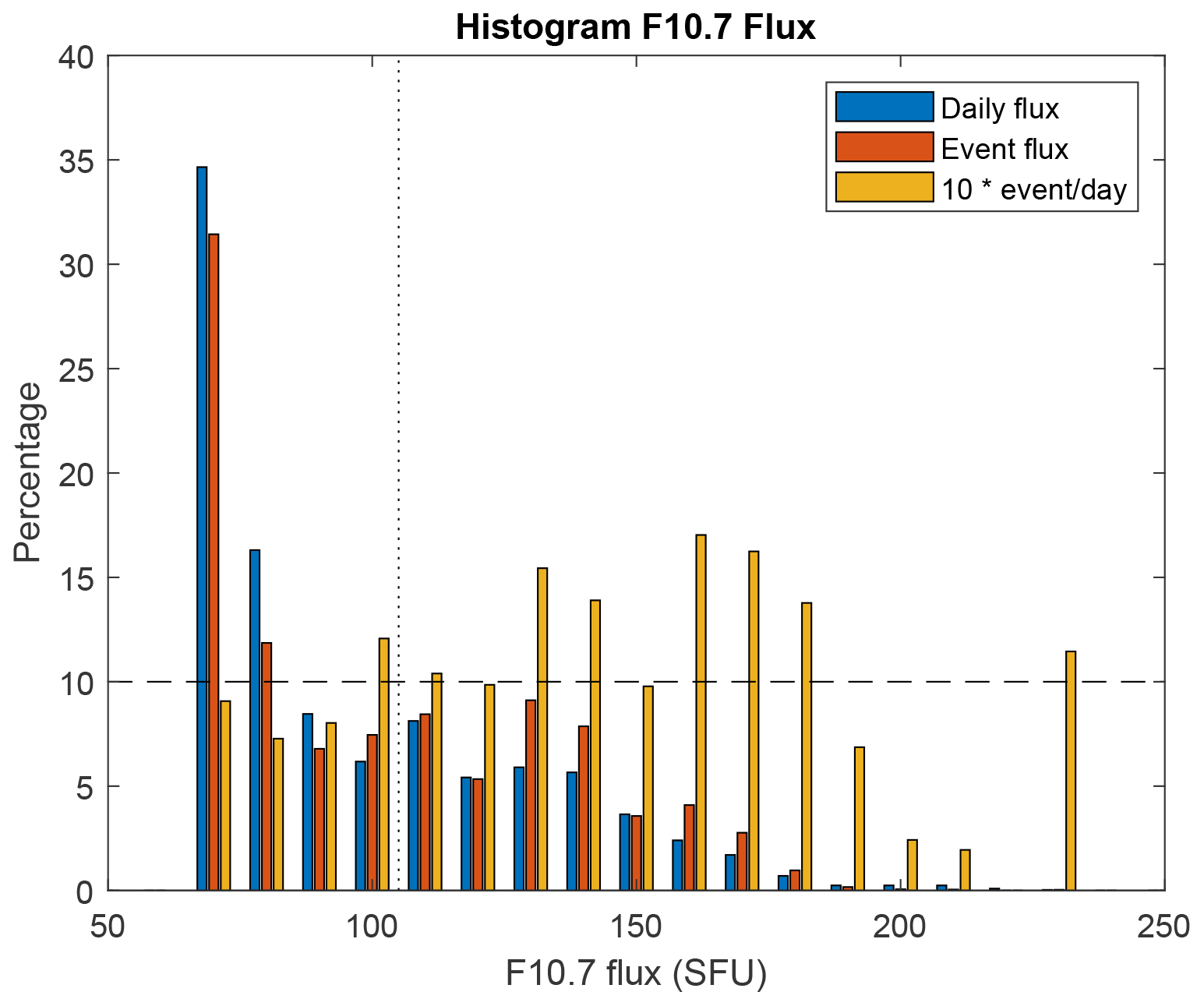
Figure 11 Histograms of the F10.7 flux. Combined are the distribution of the percentages of daily flux (blue) and of the flux for each event specifically (red). The yellow bars show the ratio of the two fluxes (yellow = red/blue, multiplied by 10 for visibility).

3.3 Dependence on bow shock characterization

In the Introduction, we stated that MMs mainly occur during periods of quasi-perpendicular bow shock conditions, as was shown in the Earth's magnetosheath by Génot et al. (2008) and at Venus by Volwerk et al. (2008c). Without a solar wind monitor upstream of Venus, it is not possible to obtain the simultaneous IMF for each event. Therefore, in this study, we have determined the IMF before the inbound and after the outbound bow shock crossing. With these upstream magnetic fields, the character of the bow shock can be obtained: quasi-perpendicular or quasi-parallel. Then, for each MM event the nearest-in-time bow shock crossing is sought to characterize under which conditions the MMs are created (for the bow shock database, see Simon Wedlund et al., 2023b).

In the overall 109 724 events for which the IMF could be determined, it was found that 81 272 (or ∼80 %) are linked to a quasi-perpendicular bow shock. How this influences the observational rate of MMs is shown in Fig. 12. Here the events are split into three groups: quasi-perpendicular with 30^∘ around the perpendicular direction to the normal, quasi-parallel with 30^∘ around the normal direction, and intermediate for the remaining 30^∘ wide bins.

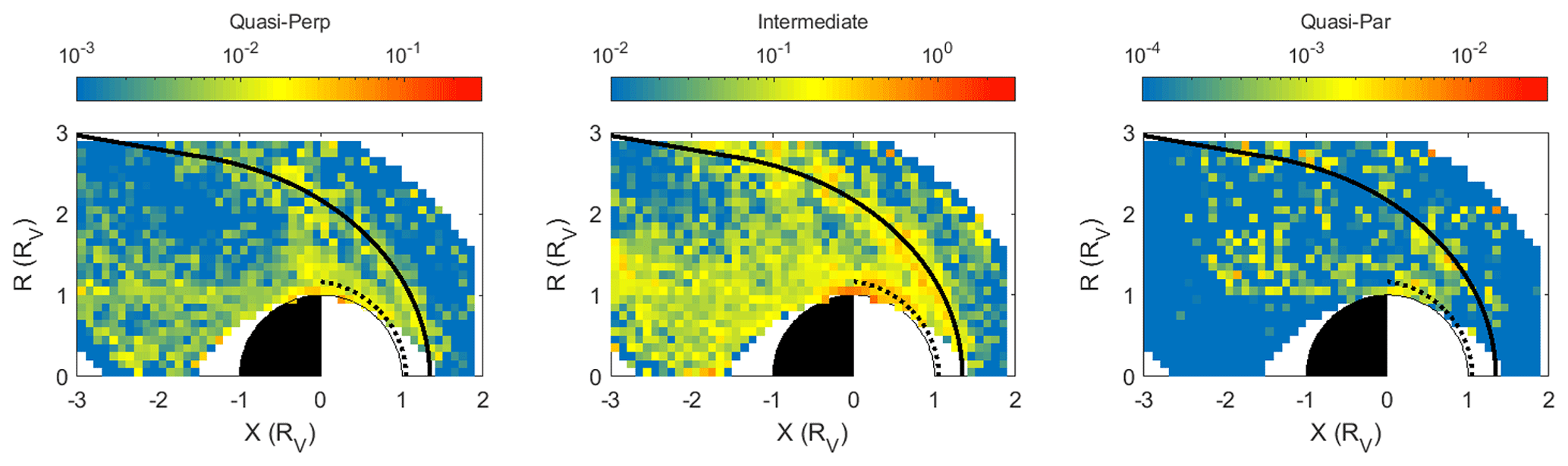
Figure 12 MM observational rate for quasi-perpendicular bow shock for reduced angle bins ($\sim \mathrm{30}{}^{\circ }$). Note that for visibility, the colour bars have different limits in each panel.

Looking at the number of events in these three categories, we find that quasi-perpendicular conditions contain ∼29 %, intermediate conditions contain ∼68 % and quasi-parallel conditions contain ∼3 % of recorded MM-like events. The observational rate of the MMs is here calculated by dividing the number of events by the reduced residence times of VEX, based on the percentage of events found. As expected, there is a very strong reduction in the observational rate for the quasi-parallel bow shock. There is also a reduction of MM-like events for the quasi-perpendicular bow shock. Interesting is the much higher occurrence of events in the intermediate category.

4 Electron density data

One of the characteristics of MMs is that there is an anti-phase between the magnetic field strength and the plasma density (see, for example,  Tsurutani et al., 1982). The magnetic-field-only CSW method to find MMs (as first proposed by Lucek et al., 1999a) needs to be tested for possible misinterpretations when plasma data are available. Rae et al. (2007) performed a study on the robustness of the method by Lucek et al. (1999a) and found that the B-field-only method, indeed, worked well. As mentioned above, Fränz et al. (2017) calculated the electron densities for the whole Venus Express mission, which we will now use to check the validity of our method.

Unfortunately, for the event on 5 May 2005 (Fig. 2) there are no electron data available, but for the near-Venus event there are (Fig. 3). In order to show the anti-phase between the magnetic field and the electron density, we have resampled the magnetic field data to the same time resolution as the electron data. In order to avoid possible offsets, we then calculated $\mathrm{\Delta }N/N$, which was then compared to $\mathrm{\Delta }B/B$ in Fig. 13.

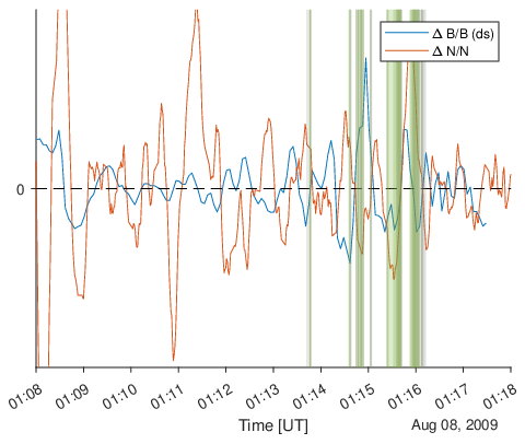
Figure 13 The magnetic field and electron fluctuations, $\mathrm{\Delta }B/B$ (blue) and $\mathrm{\Delta }N/N$ (red). The MM-active interval of Fig. 3. The anti-phase between magnetic field strength variations and electron density variations is clearly visible around the green and grey identification bars.

It is clear that $\mathrm{\Delta }N/N$ and $\mathrm{\Delta }B/B$ are in anti-phase over most of this time interval in which the CSW method determined the presence of MMs. Much of this interval was not selected by the CSW method because of the strong selection criteria. But we can see that there are regions with no anti-phase – so no MM candidates. However, there are also regions where there is an anti-phase where other strong criteria are not fulfilled, implying that we likely underestimate the total number of structures detected throughout the mission (see the discussion (Sect. 2.3.1) in Part 1 for the Mars case). Moreover, only parts of the full sinusoidal-like structure are usually captured by our algorithm, which further confirms this overall underestimation.

In order to check how the CSW method compares to the wave selection used by Fränz et al. (2017), we have also analysed 3 June 2006 (Fig. 14). Fränz et al. (2017) used the wave identification method proposed by Song et al. (1994) (also used, for example, by Ruhunusiri et al., 2015), based on the calculation of compressional and transverse wave power, plasma and magnetic pressure, and velocity variations. They find an interval of 6 min around 01:29 UT, in which there is MM activity. The green and grey lines in Fig. 14 show the identification of MMs by the CSW method and the old conditions (Volwerk et al., 2008a). There is an anti-phase between $\mathrm{\Delta }B/B$ and $\mathrm{\Delta }N/N$ at the marked locations, as well as at other non-marked locations, showing the presence of MMs. This further gives confidence to our B-field-only detection algorithm, capturing structure candidates that are indeed MMs.

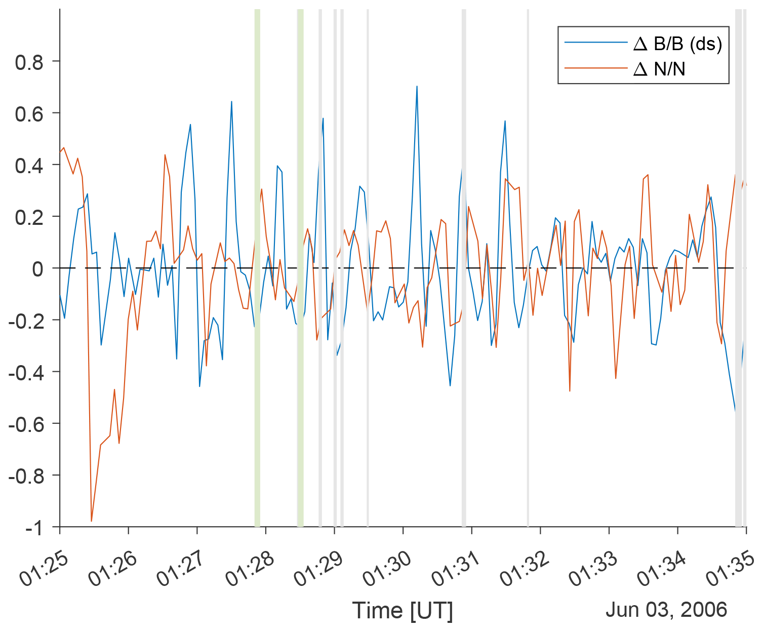
Figure 14 The MM-active interval shown by Fränz et al. (2017) in their Fig. 1 analysed with the CSW method.

5 Discussion

We have studied the probability of mirror-mode-like structures in Venus's magnetosheath over the whole Venus Express mission, with the strict constraints as presented in Part 1. The outcome can be compared to the previous study on MM-like structures by Volwerk et al. (2016) and a recent study of the plasma properties around Venus by Rojas Mata et al. (2022).

In this paper, and its companion (Simon Wedlund et al., 2023a, Part 1), we have extended the “magnetometer-only” identification method of Lucek et al. (1999a) to find the MM candidates at Mars and Venus, with mitigation strategies trying to overcome the detection of waves that may behave like MMs but in effect are not (removal of false positives in Sect. 2.2.2), called the CSW method. It is clear from this paper and from Part 1 that this is not a foolproof method, and the use of available plasma data significantly increases the accuracy of this method. Naturally, there are also other methods to determine the wave modes in magnetoplasma data, e.g. the one by Song et al. (1994), where the various ratios of magnetic field components (compressional and transverse) and plasma (pressure and velocity) are used. This method leans heavily on the knowledge of the ion-plasma data, which in the case of VEX are only available at an unsuitable resolution. The method itself has been criticized in several papers: Schwartz et al. (1996) point out that the step-wise down-selection of the wave mode is rather sensitive to an incorrect choice in the decision tree and advised the more involved analysis presented by Denton et al. (1995), and Denton et al. (1998) further critique the Song et al. (1994) method.

The whole Venus Express mission extended over most of a solar cycle, where both solar minimum and maximum are sampled well, as shown in Fig. 1 and in Table 1 for $\mathrm{\Delta }{T}_{\text{tot}}^{\text{sc}}$. There are two main differences between these two periods with respect to the MM-like structures: (1) the total number of events and probability are larger for solar maximum, and (2) the location of observations are different with the MM-like events found deeper in the magnetosheath for solar maximum.

There is a slight difference in the distribution of the depth, $\mathrm{\Delta }B/B$, of the MM-like structures for solar minimum and maximum (see Fig. 10). For solar minimum, there are more weaker MM-like structures, whereas for solar maximum there are more stronger structures. Similarly, there is a slight dependence of the observation of MM-like structures with respect to the F10.7 flux. The event flux is higher than the daily-average flux during solar maximum, whereas for solar minimum they are almost equal.

This means that only the generation of MM-like structures is strongly dependent on solar activity: more activity leads to more ionization, which in its turn leads to more ion pickup and crossings of the instability threshold (Eq. 1). But there seems to be no evolutionary development of the MM-like structures with respect to their depth – not through increased solar activity. There could be a temporal development while they are transported by the plasma flow, which will be discussed further below in Sect. 5.1.

Looking at the locations of the maxima of the probabilities 𝒫 in Figs. 7 and 8, one finds that the MM-like structures identified just behind the bow shock are deeper inside the magnetosheath for solar maximum than for solar minimum. In Fig. 8, middle panel, the bow shock location for solar minimum has also been indicated by a dashed magenta line. This panel shows that the maximum probability is at the location of this magenta line. It is unclear whether this is just by chance or if this location has a physical meaning.

5.1 Comparison with Volwerk et al. (2016)

Mirror modes in Venus's magnetosheath were first discovered by Volwerk et al. (2008b, c), and a comparison between solar minimum and solar maximum was presented in Volwerk et al. (2016). These studies, however, were based on only 1 Venus year (223 Earth days) of data for each solar activity level. Nevertheless, some of the results from those papers are in agreement with the results presented above for the full 2006–2014 VEX dataset.

Figure 3 in Volwerk et al. (2016) shows the occurrence rate of the MM-like structures on a coarser grid of 0.25×0.25R_V. Note that the definition of the occurrence rate in the papers by Volwerk et al. (2016) is different than in our present study. They gathered together closely spaced intervals to obtain MM events, separated by at least 30 s, whereas in our study the total number of seconds for which the MM conditions are fulfilled is used. We expect that these different ways of assessing MM-like structures are still comparable on average. It is clear that these plots show less structure than the middle panels of Figs. 7 and 8 because of the lesser amount of data and the coarser grid. We will compare a few of their conclusions with the results in the present study. Volwerk et al. (2016) state the following:

1. The number of MM-like structures at solar maximum is higher than at solar minimum by ∼14 %;

2. The probability is the same for solar minimum and maximum conditions;

3. The distribution of $\mathrm{\Delta }B/B$ is exponential with approximately the same coefficient for both solar conditions;

4. For solar minimum, the general trend for MM-like structures is to decay; for solar maximum, MM-like structures first grow and then decay, between the bow shock and the terminator;

Point (1) is in general agreement with what is shown in Table 1, albeit that the increase for solar maximum is ∼45 %, even though the total residence time for solar maximum was ∼10 % less. This again has an influence on point (2), regarding the probability. In our present study, we find that in total the probabilities of detection of MM-like structures are ∼0.05 and ∼0.08 for solar minimum and maximum (Table 1), respectively, i.e. a multiplication factor of ×1.6, between solar minimum and solar maximum conditions. This shows that considering a larger statistical dataset for this kind of study greatly influences the statistical results.

Figure 10 shows the distribution of $\mathrm{\Delta }B/B$, which seems to indicate an exponential drop-off as in point (3). Volwerk et al. (2016) found two different e-folding lengths, b, through a fit:

$$\begin{array}{}\text{(7)}& y=a\times \exp \mathit{\{}b\times \mathrm{\Delta }B/B\mathit{\}},\end{array}$$

describing the distribution for “weak” ($\mathrm{\Delta }B/B<\mathrm{0.6}$) and “strong” ($\mathrm{\Delta }B/B>\mathrm{0.4}$) MM-like structures,⁴ with $b\approx -\mathrm{3.4}$ and $b\approx -\mathrm{2.5}$, respectively, for solar minimum and maximum conditions. In our present study the data seem to also show an exponential decay but with three slopes (see Fig. 15): $b\approx -\mathrm{9.9}$, $b\approx -\mathrm{5.4}$ and $b\approx -\mathrm{10.5}$. This significantly differs from earlier results.

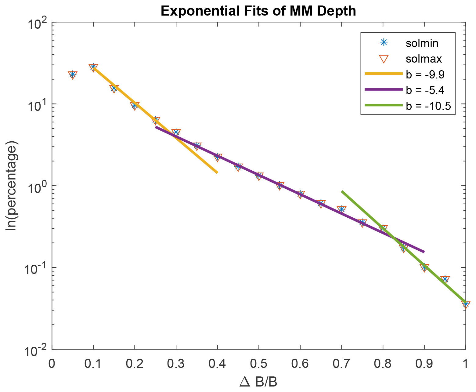
Figure 15 Exponential fits to the depth distribution of the MM-like structures for solar minimum and maximum. Three different regions can be identified and the slopes b for the fits $y=a\times \exp \mathit{\{}b\times \mathrm{\Delta }B/B\mathit{\}}$ can be found in the legend.

Looking at the distribution of the occurrence rate, as well as fitting the median and upper/lower quartiles of $\mathrm{\Delta }B/B$ taken in 0.25R_V bins, Volwerk et al. (2016) found that for solar minimum there was a decrease of these numbers from the bow shock away, whereas for solar maximum these values were first increasing and then decreasing.

In Fig. 16, we first calculate the distance of any event on the map to the bow shock along the X_VSO line, with R=constant. $\mathrm{\Delta }B/B$ is plotted for three R intervals. The vertical red lines show the average location of the terminator with respect to the shock. In the panels, the mean (red) and standard deviation (green) are overlaid. There is an increase in the depth of the structures towards the terminator and slightly behind, although in the bottom panels for $\mathrm{1.0}\le R\le \mathrm{1.2}$ this is not quite visible in the mean and standard deviation.

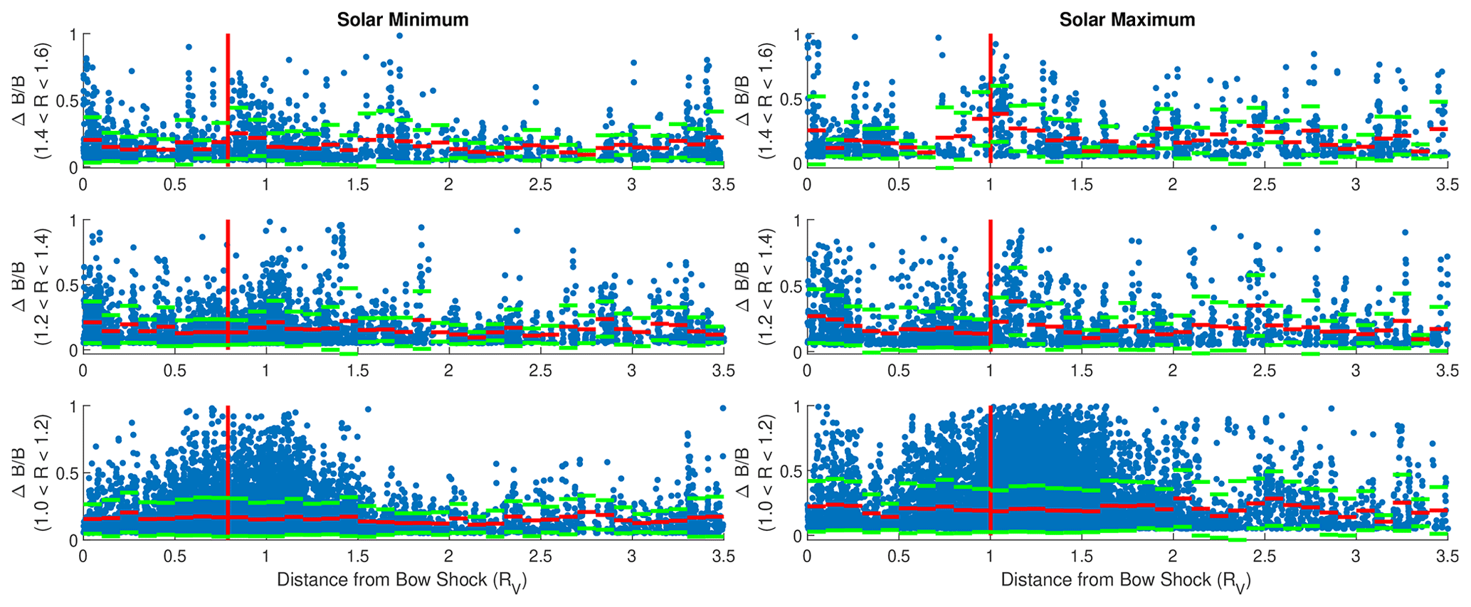
Figure 16 $\mathrm{\Delta }B/B$ as a function of distance from the bow shock for three intervals: $\mathrm{1.0}\le R\le \mathrm{1.2}$, $\mathrm{1.2}\le R\le \mathrm{1.4}$ and $\mathrm{1.4}\le R\le \mathrm{1.6}$. The vertical red line shows the distance of the terminator to the bow shock in the $\mathrm{1.0}\le R\le \mathrm{1.5}$ bin.

This is different from Volwerk et al. (2016), where it was stated that the MM-like structures decay away from the BS at solar minimum and first grow and then decay at solar maximum. With better statistics, this is not the case, there is a drop in maximum $\mathrm{\Delta }B/B$ from the BS inward, i.e. from 0 to ∼0.25R_V, for both situations.

A point not discussed in Volwerk et al. (2016) but well-investigated in Volwerk et al. (2008c) is the role of the bow shock characterization. It is expected that the MMs are mainly generated behind a quasi-perpendicular bow shock (where the crossing ions are mainly heated in the perpendicular direction to the magnetic field) and close to the magnetic pileup region close to the planet (through conservation of the first adiabatic invariant), from which they then are transported by the plasma flow. Figure 6 in Volwerk et al. (2008c) shows the occurrence rate in the dayside magnetosheath for various angle ranges between the IMF and the bow shock normal. It shows clearly that the occurrence rate drops significantly when the bow shock is quasi-parallel. Above in Fig. 12 a similar effect is observed. The split into three bins (quasi-perpendicular, intermediate and quasi-parallel) shows that for the latter there are almost no events (∼3 %) and that most of the events are found in the intermediate group (∼68 %).

5.2 Comparison with Rojas Mata et al. (2022)

Lately, Rojas Mata et al. (2022) have studied the Ion Mass Analyser (IMA) proton data of the ASPERA-4 instrument, showing the proton temperature anisotropies during the whole VEX mission, divided up into solar minimum and maximum, similarly as in our present study. In Fig. 17 the temperature ratio $\mathcal{T}=\text{median}(T_{⟂}/T_{\Vert })$ for each grid cell is shown on a smaller grid (0.1×0.1R_V) than in the original paper. The overall trends are similar for both grid resolutions except a few random “outlier-looking” bins. It was found that the highest temperature anisotropy, 𝒯, lies deeper inside the magnetosheath for solar maximum. Indeed, the same conclusion can be made from Fig. 17, where, like in the occurrence rate in Fig. 8, we have plotted the solar minimum location of the bow shock as a dashed magenta line. Interestingly, this line seems to lie well along the boundary of the maximum 𝒯.

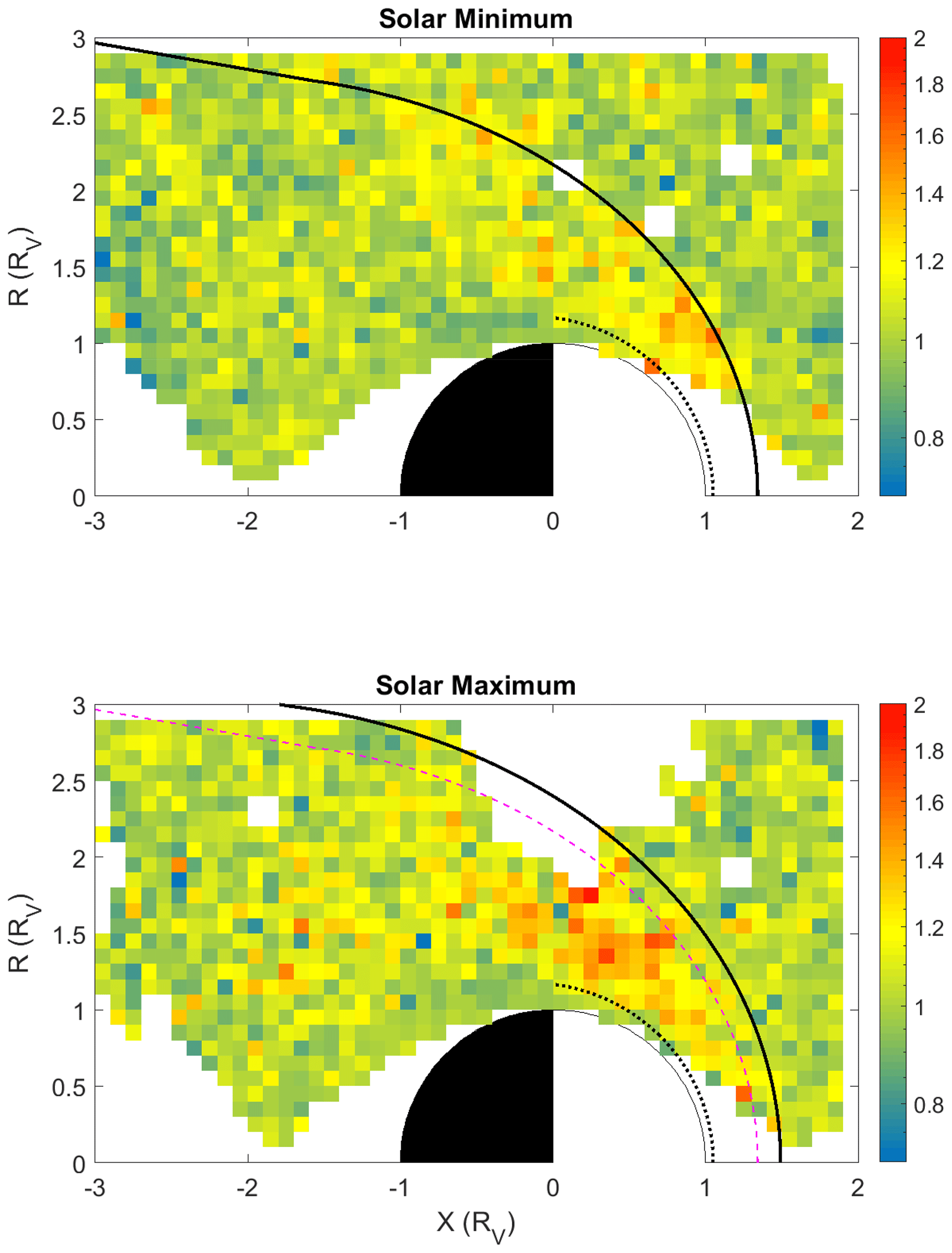
Figure 17 The temperature ratio $\mathcal{T}=\text{median}(T_{⟂}/T_{\Vert })$ for each grid box around Venus for solar minimum (top) and maximum (bottom). The data have been re-evaluated on a 0.1×0.1R_V grid from the study by Rojas Mata et al. (2022).

It should be noticed that there is a bias in the comparison between the ASPERA-4 data, with 192 s resolution and the magnetometer resolution of 1 s. The ion data will show larger local variations as with the orbital velocity of VEX of ∼8 km s⁻¹; this results in a size of ∼1500 km or ∼0.25R_V (the tentative reason to have this grid cell size in Rojas Mata et al., 2022), although this does not take into account the (much) faster plasma flow in the magnetosheath. However, the averaging done in the grid cells might reduce this effect slightly in the statistics.

When comparing the 𝒫 distributions in the middle panels of Figs. 7 and 8 with 𝒯 in Fig. 17, one notices that, as said above, there are two regions of maximum 𝒫, whereas the maximum of 𝒯 seems to fall between these two regions. The effect is most clearly visible for solar maximum conditions. This shows that the presence of MM-like structures locally reduces the (median) temperature ratio, 𝒯, in the magnetosheath, an indication that the instability transfers its energy from the ions to the waves.

Figure 18 shows the percentage of scans in each 0.1×0.1R_V cell, for which the instability criterion MMI<0 (Eq. 1) is fulfilled. Note the large difference between the two solar conditions: although the criterion is fulfilled much more frequently at solar minimum than at solar maximum, there are fewer MM-like structures on average as shown in Figs. 7 and 8. This points at an extra necessity for MM-like structures to start to develop, apart from the instability criterion of Eq. (1).

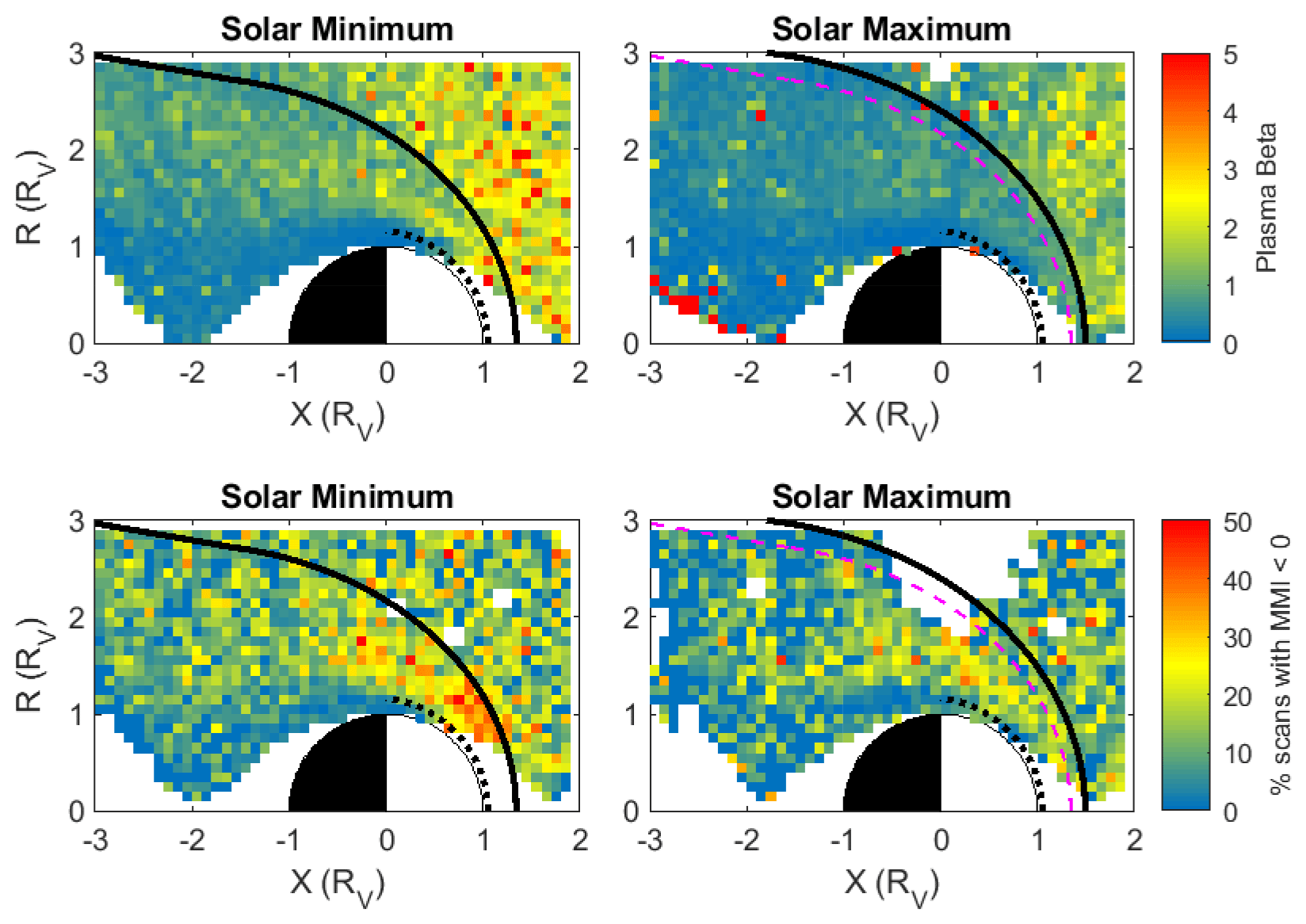
Figure 18 Top: the mean plasma beta (β) in Venus's environment. Bottom: the percentage of scans in each box for which the instability criterion, Eq. (1), MMI<0 holds. The data have been re-evaluated on a 0.1×0.1R_V grid from the study by Rojas Mata et al. (2022).

6 Conclusions

We have studied the magnetic field data for the whole Venus Express mission and searched for mirror modes in the magnetosheath. The VEX mission has been split up into two parts, corresponding to solar minimum and solar maximum, for which one of the main differences is that the bow shock for solar maximum is further out at ∼1.49R_V as compared to ∼1.34R_V for solar minimum at the subsolar point.

The total probability 𝒫 for solar maximum lies higher than for solar minimum even when normalizing to the total observation time for each condition. The regions where the MM-like structures are observed are behind the BS and near the magnetopause/ionopause. But behind the BS, the probability 𝒫 peaks further inside the magnetosheath for solar maximum. Comparison with the proton data shows that 𝒫 peaks where the temperature anisotropy, 𝒯, is reduced, indicating that energy has been transferred from the ions to the waves.

The total probability 𝒫 is lower for solar minimum than for solar maximum (Table 1), but Fig. 18 shows that the percentage of scans with MMI<0 is larger for solar minimum. Again, this raises the question of whether there is more to the creation of MM-like structures than just the instability criterion. The major difference in the two periods is the plasma beta (β), shown in Fig. 18 (top panels), which is much higher for solar minimum (as also observed by Wilson et al., 2018, in the solar wind at 1 au). This extra thermal energy does not seem to drive more or even deeper MM-like structures as shown in Fig. 10. Quite possibly, there is a competing effect: Rojas Mata et al. (2022) show that there is a higher compression of the IMF during solar maximum in the dayside magnetosheath. This would decrease β, but through the first adiabatic variant mechanism it could increase the perpendicular temperature and thereby increase β and the anisotropy. Indeed, in the magnetosheath behind the quasi-perpendicular bow shock an inverse correlation was found with variations between high β – low temperature anisotropy – and low β – high temperature anisotropy (Anderson and Fuselier, 1993, 1994; Anderson et al., 1994; Fuselier et al., 1994).

The distribution of the depth of the MM-like structures does not seem to be strongly dependent on solar conditions. The distribution seems to be exponential, but closer inspection shows a combination of three different exponential slopes, with no difference between solar minimum and maximum. Also, solar irradiance, with its proxy the F10.7 flux, does not seem to influence the number of MM-like structures.

There remain some open questions after this study. Why are there large regions where the temperature anisotropy, 𝒯, is enhanced and the MM probability, 𝒫, reduced? (This could be due to the difference between generation region and region of observation. Starting with a high anisotropy and creating MMs, by the time they are observed, the structures have already been transported downstream before they have had the chance to dissipate the free energy.) What are the extra conditions for MM-like structures to start to grow in the magnetosheath plasma? And What is the dependence on solar wind IMF conditions? Also, the location of the solar minimum bow shock seems to take a special place, as during solar maximum it is the boundary where the probability, 𝒫, strongly increases.