the Creative Commons Attribution 4.0 License.
the Creative Commons Attribution 4.0 License.
 | 31 May 2023
Statistical distribution of mirror-mode-like structures in the magnetosheaths of unmagnetised planets – Part 1: Mars as observed by the MAVEN spacecraft
Cyril Simon Wedlund
Martin Volwerk
Christian Mazelle
Sebastián Rojas Mata
Gabriella Stenberg Wieser
Yoshifumi Futaana
Jasper Halekas
Diana Rojas-Castillo
César Bertucci
Jared Espley
In this series of papers, we present statistical maps of mirror-mode-like (MM) structures in the magnetosheaths of Mars and Venus and calculate the probability of detecting them in spacecraft data. We aim to study and compare them with the same tools and a similar payload at both planets. We consider their dependence on extreme ultraviolet (EUV) solar flux levels (high and low) and, specific to Mars, on Mars Year (MY) as well as atmospheric seasons (four solar longitudes Ls). We first use magnetic-field-only criteria to detect these structures and present ways to mitigate ambiguities in their nature. In line with many previous studies at Earth, this technique has the advantage of using one instrument (a magnetometer) with good time resolution, facilitating comparisons between planetary and cometary environments. Applied to the magnetometer data of the Mars Atmosphere and Volatile EvolutioN (MAVEN) spacecraft from November 2014 to February 2021 (MY32–MY35), we detect events closely resembling MMs lasting in total more than 170 000 s, corresponding to about 0.1 % of MAVEN's total time spent in the Martian plasma environment. We calculate MM-like occurrences normalised to the spacecraft's residence time during the course of the mission. Detection probabilities are about 1 % at most for any given controlling parameter. In general, MM-like structures appear in two main regions: one behind the shock and the other close to the induced magnetospheric boundary, as expected from theory. Detection probabilities are higher on average in low-solar-EUV conditions, whereas high-solar-EUV conditions see an increase in detections within the magnetospheric tail. We tentatively link the former tendency to two combining effects: the favouring of ion cyclotron waves the closer to perihelion due to plasma beta effects and, possibly, the non-gyrotropy of pickup ion distributions. This study is the first of two on the magnetosheaths of Mars and Venus.
- Article
(7339 KB) - Full-text XML
- Companion paper
- BibTeX
- EndNote


Mirror modes (MMs) are magnetic bottles of various sizes and shapes containing high-density plasma drifting with the ambient plasma. They are often found in the magnetosheaths of solar system objects, either magnetised like Earth (e.g. Lucek et al., 1999; Ala-Lahti et al., 2018, and references therein) or weakly to non-magnetised like comets (Mazelle et al., 1991; Glassmeier et al., 1993), Venus (see Volwerk et al., 2016, and references therein) and Mars (see Simon Wedlund et al., 2022b, and references therein).
Arising from plasma microinstabilities themselves triggered by an ion temperature anisotropy in the plasma, MM waves are compressional, essentially linearly polarised, ultra-low-frequency (ULF), long-wavelength transverse waves which are non-propagating in the plasma rest frame (Gary, 1992). The drift MM instability is typically triggered in a weakly magnetised plasma (that is, in a high plasma beta β≫1), a condition that is met in a planetary magnetosheath, whereas the Alfvén ion cyclotron instability takes over for low plasma-β conditions. The MM instability is expected to grow when the MM instability criterion (MMI) is fulfilled for a plasma composed of charged species i (Hasegawa, 1969):
where subscripts ∥ and ⟂ denote the directions parallel and perpendicular to the ambient magnetic field direction Bbg. The species temperature is noted Ti, and the perpendicular plasma beta βi⟂ measures the competing effects of plasma and magnetic pressures so that , with Ni representing the species density.
Several mechanisms at the origin of the temperature anisotropy have been proposed (Gary, 1993). At every object with a well-defined bow shock (Earth, Mars, Venus and comets nearing perihelion), the quasi-perpendicular (noted “Q-⟂”) shock provides in its wake a preferential heating of the ions along the perpendicular direction to the magnetic field, favouring the generation of MMs. Another possibility exists, specific to environments with weak gravity (Mars, Venus, comets): in their extended exosphere, ions created by photoionisation are picked up by the solar wind (Szegö et al., 2000). In the plasma rest frame, the velocity distribution function of these pickup ions takes the form of an unstable ring-beam distribution, with the relative value of both parallel and perpendicular components depending only on the local cone angle between the B field and the bulk plasma velocity vector at the location of the ionisation. For large-enough cone angles, the ring component of the distribution results in an ion temperature anisotropy , which is a source of free energy for microinstabilities such as MMs (Price, 1989).
Because of their stationary nature, MMs can be convected downstream of their birth place, likely unchanged, by their surrounding plasma. As a consequence, many structures end up piling up against the magnetospheric boundary in the deep magnetosheath, where they are finally detected, as, for example, shown by Earth observations close to the magnetopause (Erkaev et al., 2001).
In spacecraft data, the signature of MMs takes the form of sudden dips or peaks in the magnetic field intensity in antiphase with plasma density variations, lasting a few seconds to tens of seconds. Considering that spacecraft are essentially at rest with respect to the ambient plasma and for plasma speeds of the order of 100 km s−1, their sizes are at Mars of the order of a not insignificant fraction of a planetary radius RM=3389.5 km. In addition, MMs likely share a common ancestor with magnetic holes (MHs), which are isolated magnetic field depressions usually found in the upstream solar wind (e.g. Volwerk et al., 2021; Madanian et al., 2020, and references therein) or in the magnetosheath of planets (e.g. Karlsson et al., 2021).
Traditionally, several ways of detecting MM structures have been used. The most widespread and easiest method is to use magnetic-field-only measurements with ad hoc criteria constraining the compressibility and the quasi-linear polarisation of the detected structures (Soucek et al., 2008; Génot et al., 2009). It has the advantage of using a well-calibrated instrument, the magnetometer, that has been flown on many space missions and has a high temporal resolution, good accuracy and excellent reliability over an extended mission lifetime. However, ambiguities in the nature of the detected structures always remain: for example, highly compressional structures may meet all B-field criteria without necessarily fulfilling the MMI or the B–N anticorrelation behaviour, pointing to other types of waves (Song et al., 1994). Moreover, the criteria chosen are somewhat arbitrary and may either include many false positive detections or miss altogether most of the events if too stringent. Most of these ambiguities can at least be partially lifted with the use of dedicated plasma measurements (Gary and Winske, 1992).
A complementary approach is to use the property of MMs of having variations in B and plasma density Np in antiphase. One caveat is that plasma measurements need to have sufficient temporal resolution to be able to capture structures not lasting more than a few tens of seconds: many ion instruments on earlier planetary space missions such as Mars Express or Venus Express (VEX) have a 192 s scanning rate, which is much too low to be of help. Electron measurements can fare better: at Mars, for example, Bertucci et al. (2004) looked instead at the B–Ne antiphase behaviour (Ne being the electron density) of highly compressional linear structures to argue in favour of MMs. This was also because no ion instrument was flown on Mars Global Surveyor (MGS). Recently, a new study by Jin et al. (2022) has taken advantage of the B–N criterion with magnetometer and ion instruments used in combination to detect MM-like structures across the first 4 years of measurements with MAVEN (Mars Atmosphere and Volatile EvolutioN). They remarked that most structures likely form at the bow shock, where they take the shape of peaks or that of a mix of peaks and dips, with the latter in agreement with the case study results of Simon Wedlund et al. (2022b).
A separate approach using plasma measurements and magnetic field data relies on the hierarchical scheme of Gary and Winske (1992) and Song et al. (1994) based on so-called “transport” ratios that formalise correlations in Fourier space between magnetic field and plasma pressure. This method is well suited for statistical surveys and has successfully been used at Mars by Ruhunusiri et al. (2015) and at Venus by Fränz et al. (2017). Both studies presented two-dimensional maps of the distribution of low-frequency wave modes, showing that MMs are present in the magnetosheath and magnetotail at probabilities of less than 20 %, whereas the bulk of the wave activity is contained in the Alfvén and quasi-parallel slow modes. This method is dependent on the plasma measurements and their Fourier analysis, which makes use of rather large temporal windows to be computationally feasible. Moreover, it is based on magnetohydrodynamic considerations, which may not be entirely reliable for kinetic microinstabilities (Schwartz et al., 1997).
Alternatively, and to lift most ambiguities, the precise study of the MMI, with the derivation of robust ion and electron temperature anisotropy estimates at enough time resolution to be relevant to MMs, is ideally the best way of characterising MMs. This remains, however, to this day a challenging task more suited to case studies. Such an in-depth characterisation of MMs was for the first time made by Simon Wedlund et al. (2022b). It was made possible by the arrival in 2014 at Mars of the Mars Atmosphere and Volatile EvolutioN (MAVEN) spacecraft, which carries magnetometer (Connerney et al., 2015) and high-time-resolution plasma instruments, such as the Solar Wind Ion Analyzer (SWIA; Halekas et al., 2015) and the Solar Wind Electron Analyzer (SWEA Mitchell et al., 2016). Simon Wedlund et al. (2022b) described a classical event in December 2014 at the end of Mars Year 32 (MY32) containing a train of MMs lodged against the induced magnetospheric boundary (IMB). From considerations of the MMI and the size of these structures, the authors argued for a remote generation region in the immediate wake of the Q-⟂ bow shock, in a way similar to Earth observations (see Erkaev et al., 2001). With MAVEN, Halekas et al. (2017a) presented for the first time maps of the distribution of the temperature anisotropy at Mars using the maximum temperature perpendicular to the ambient magnetic field. Predictably, the Martian magnetosheath exhibits a strong anisotropy especially at regions controlled by the Q-⟂ shock for low Mach numbers. These anisotropies are especially conducive to the growth of MMs and Alfvén ion cyclotron waves.
We aim in this series of papers to provide for the first time occurrence probability maps in different conditions at Mars (present paper, abbreviated Part 1) and Venus (Part 2, Volwerk et al., 2022) using the same method of investigation. For simplicity, reproducibility and to allow for future comparisons at other solar system objects such as comets, we opt for a magnetic-field-only analysis in the same way as Volwerk et al. (2008, 2016) using the magnetometers on board MAVEN and VEX. Contrary to Venus, no long-term statistical study has ever been dedicated to MMs at Mars, a gap we propose to address here. In this way, we have the unique chance of directly comparing planets with the very same detection criteria, here based on, for example, the recommendations of Simon Wedlund et al. (2022b). Although ambiguities do remain regarding the nature of the detected structures, such a comparison remains meaningful as long as we are careful to remove false positive candidate structures that are obviously not MMs. Such work will serve as a basis for re-evaluating past datasets at Mars, Venus and comets.
In Sect. 2, we present our method of detection of MM-like events at Mars, based on B-field-only criteria determined statistically from a subset of carefully chosen data. After describing techniques to mitigate the presence of false positive detections (Sect. 2.2.2), we apply the B-field-only criteria to the whole MAVEN magnetometer dataset between November 2014 and February 2021, covering four Mars Years, MY32 to MY35 included (Sect. 2.2.3). We proceed to create 2D maps of MM-like events normalised by the spacecraft residence time, which are in effect a probability to observe MM-like structures within a given grid cell (Sect. 2.3). We then study and discuss in Sect. 3 the dependence of these probabilities on several physical parameters of interest, such as Mars Year (MY), solar extreme ultraviolet (EUV) flux and Mars season, parameterised by the solar longitude Ls. For simplicity in this first comparative study based on a magnetic-field-only perspective, solar wind drivers such as dynamic pressure, interplanetary magnetic field configuration and strength or nature of the shock are left for future work. We conclude our present study with suggestions for improvements and new controlling parameters to explore (Sect. 4).
2.1 Instrumentation
We use for this study the magnetic field investigation package on board MAVEN (abbreviated MAG in the following), which consists of two triaxial fluxgate magnetometers mounted at the extremity of boomlets on the spacecraft's solar panels (Connerney et al., 2015). It allows for the measurement of the 3 components of the magnetic field with a nominal frequency of 32 Hz and an accuracy better than 0.05 %. Because the structures we are looking for in the dataset are expected to last from a few seconds up to 15–20 s (Simon Wedlund et al., 2022b), the high time resolution of the instrument is downsampled to 1 s .
As supporting instrument for the event cases shown in Figs. 1 and 2 (last panel), we use MAVEN's Solar Wind Ion Analyzer (SWIA) electrostatic ion analyser, which measures ion differential fluxes with a maximum temporal resolution of 4 s (Halekas et al., 2015). Specific modes are available depending on energy/angle scanning and telemetry modes; we considered two modes here: SWICA (SWIA Coarse Archive, 8 s resolution), suited to magnetosheath conditions, and SWIFA (SWIA Fine Archive, 4 s resolution), designed for the monitoring of solar wind ions. Density moments are manually calculated from SWICA and SWIFA modes depending on the region considered.
2.2 Detection method
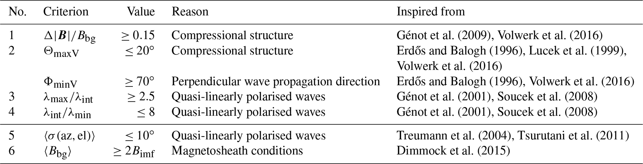
The detection of MM-like structures is based on spacecraft magnetometer data using magnetic-field-only criteria. This has the advantage of a faster and unified detection across planets such as Mars or Venus, at the expense of the certainty that these detections are MM proper. We follow here the recommendations of Simon Wedlund et al. (2022b). These authors first used magnetic field and plasma data in coincidence to identify the unmistakable signature of a train of MMs during the early part of the mission and could then validate a set of B-field-only criteria to closely match these observations. Their rearranged series of criteria are listed in Table 1 for convenience. These criteria assume that the sought structures are compressional in nature (Criterion 1) and that they are quasi-linearly polarised (Criteria 2–4). Criteria 1–4 need to be simultaneously fulfilled in order for a MM-like event to be selected. After the initial detection, additional constraints can be put on the found intervals such as Criterion 5 (quasi-linear polarisation) and Criterion 6 (presence in the magnetosheath as opposed to in the solar wind). We briefly describe these criteria in Sect. 2.2.1, as the reader is referred to Simon Wedlund et al. (2022b) (and references therein) for further consideration and motivation regarding the specific values chosen for each criterion.
Because the method is based only on criteria on the magnetic field and not on a more involved plasma data analysis, the possibility of false positive detections exists: we describe steps to mitigate this aspect in Sect. 2.2.2, with caveats discussed in Sect. 2.2.3. Consequently, the events we are expected to capture here are candidate MMs, dubbed mirror-mode-like in the following (“MM-like”), to use the original nomenclature of Volwerk et al. (2008) at Venus. Moreover, we refer in the following to the detections as “events” as we go through each 1 s of magnetic field data, whereas “structures” refer to a MM-like fluctuation as a whole (a dip or a peak, or a mix of them, as in Joy et al., 2006), which may contain several detected events. When accumulating detection events in a statistical spatial grid, the detection probability will simply be referred to as “probability of MM-like structures”.
Génot et al. (2009)Volwerk et al. (2016)Erdős and Balogh (1996)Lucek et al. (1999)Volwerk et al. (2016)Erdős and Balogh (1996)Volwerk et al. (2016)Génot et al. (2001)Soucek et al. (2008)Génot et al. (2001)Soucek et al. (2008)Treumann et al. (2004)Tsurutani et al. (2011)Dimmock et al. (2015)Table 1Magnetic-field-only criteria for detecting MM-like structures (adapted from Simon Wedlund et al., 2022b): magnetic field fluctuation (Criterion 1); MVA angles ΘmaxV (ΦminV) between maximum (minimum) variance direction and that of Bbg (Criterion 2); ratio of MVA eigenvalues () between maximum (intermediate) and intermediate (minimum) eigenvalues (Criteria 3 and 4); moving standard deviation of magnetic azimuth and elevation angles 〈σ(az,el)〉 (Criterion 5) and average background field over a 2 min interval (Criterion 6). We use most of the revised set of values in Simon Wedlund et al. (2022b), except for changed to 0.15 and ΘmaxV changed from ≤23∘ to for symmetry. The angular variation across a train of events is estimated by calculating the moving standard deviation noted 〈σ(az,el)〉 over a 2 min period (in accordance with the background field calculations); because angular variations in magnetic field azimuth and elevation need to be kept below for linearly polarised structures, we choose here .
2.2.1 B-field-only criteria
First, we estimate the background magnetic field intensity Bbg using a low-pass Butterworth filter as in Volwerk et al. (2016) for Venus and Simon Wedlund et al. (2022b) for Mars. We adopt a 2 min window ( Hz), a passband ripple of 2 dB and a stopband attenuation of 20 dB.
Criterion 1 ensures that the structure is compressional with an absolute B-field fluctuation of:
that is, magnetic field fluctuations are larger than or equal to 15 % of the background field. To obtain criteria 2–4, we then perform a moving minimum variance analysis (noted MVA; see Sonnerup and Scheible, 1998) with a 15 s moving window, which is about the width of the larger MM structures found at Mars (Simon Wedlund et al., 2022b), and a shift of 1 s. From the MVA, we define two angles: ΘmaxV (ΦminV) is the angle between the maximum (minimum) variance eigenvector direction and that of the background magnetic field. A small (large) enough angle denotes also a compressional wave with propagation in the direction perpendicular to B (Erdős and Balogh, 1996), as expected and shown in the kinetic MM simulations of Price et al. (1986). We use also the ratio of the maximum-to-intermediate eigenvalues (intermediate-to-minimum eigenvalues ) to further constrain the shape of the variance ellipsoid into a cigar-shaped one (quasi-linear polarisation; see Génot et al., 2001, and references therein).
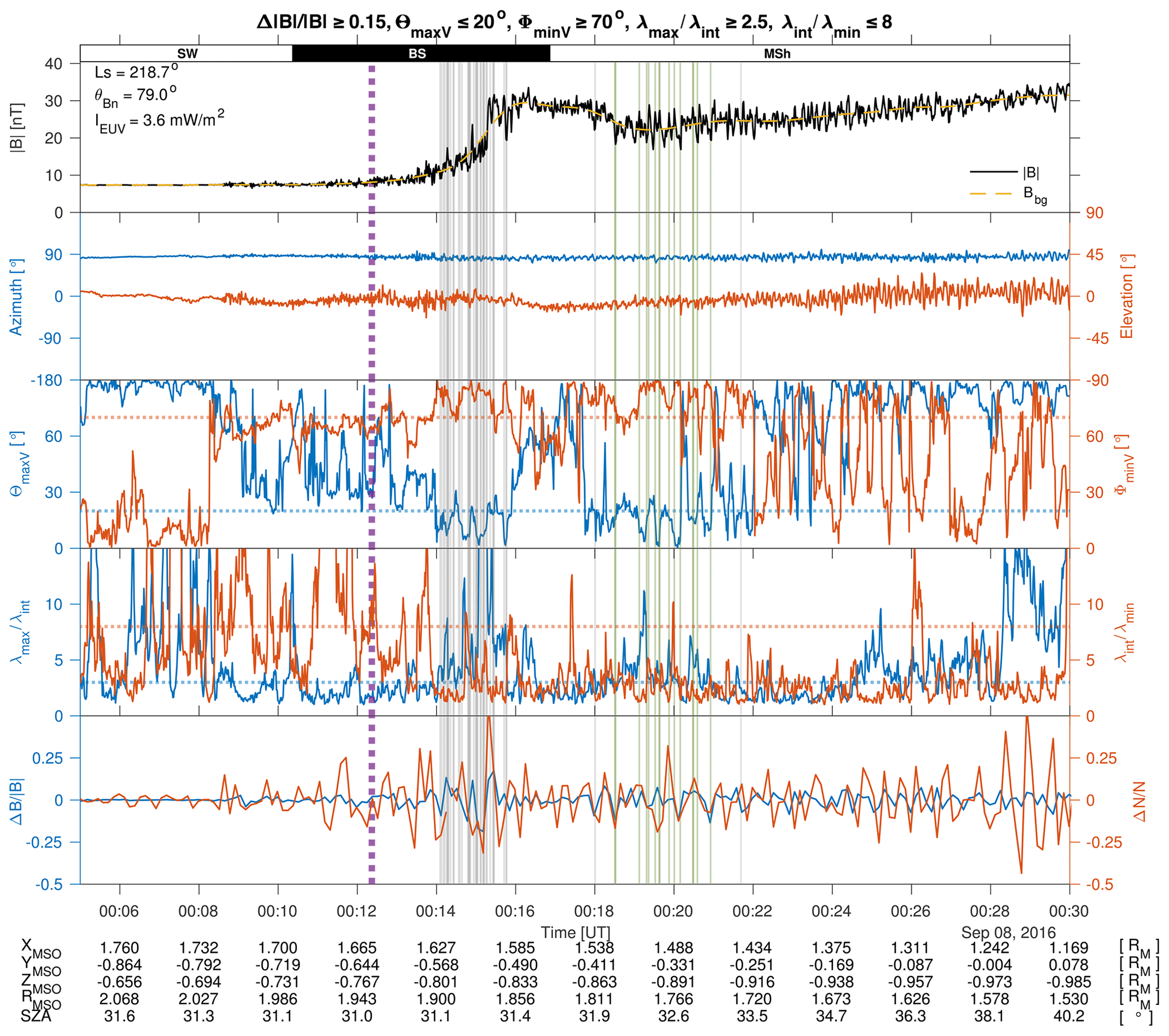
Figure 1Example of MM-like detections at Mars, using the B-field-only criteria of Table 1 on 8 September 2016, at relatively high solar activity. From top to bottom: total magnetic field strength, with Bbg being the background magnetic field calculated as a Butterworth low-pass filter over 2 min; magnetic field azimuth (left axis) and elevation (right axis) angles; MVA angles between the maximum (minimum) variance eigenvector direction ΘmaxV and that of the background B field on left axis (ΦminV on right axis). The threshold values for selections of MMs are indicated by blue and red dotted lines for each respective angle; MVA eigenvalue ratios on left axis (, right axis), with their respective thresholds in dotted lines; magnetic field and ion density variations so that and need to be in antiphase with respect to 0 for a typical MM behaviour. We downsample the magnetic field variations to the resolution of that of the ion instrument and calculate the background density Nbg using the same Butterworth filter as for B. In the solar wind before 00:15 UT, the SWIFA mode (4 s resolution) of SWIA is chosen for the calculation of the density moment variation, whereas afterwards the SWICA mode is preferred (8 s resolution) as per the recommendation of Halekas et al. (2017b). We indicate below the figure XMSO, YMSO, ZMSO, radial distance RMSO in units of Mars' radius RM, and solar zenith angle . Solar longitude was , and average solar EUV flux 〈IEUV〉≈3.6 mW m−2. The angle θBn between the bow shock normal and the interplanetary magnetic field direction was determined to be (reminiscent of Q-⟂ bow shock conditions) assuming a smooth shock geometry as explained in Simon Wedlund et al. (2022a). The original detections using Criteria 1–4 of Table 1 appear as grey and vertical green lines, with the green portion representing the final detections with removal of false positives (Criteria 1–4 and 5–6, and Sect. 2.2.2). The start position of the bow shock region in dotted purple is estimated through the predictor–corrector algorithm of Simon Wedlund et al. (2022a). To replace this event in MAVEN's timeline of EUV activity and Ls ranges, see first orange dot in Fig. 4.
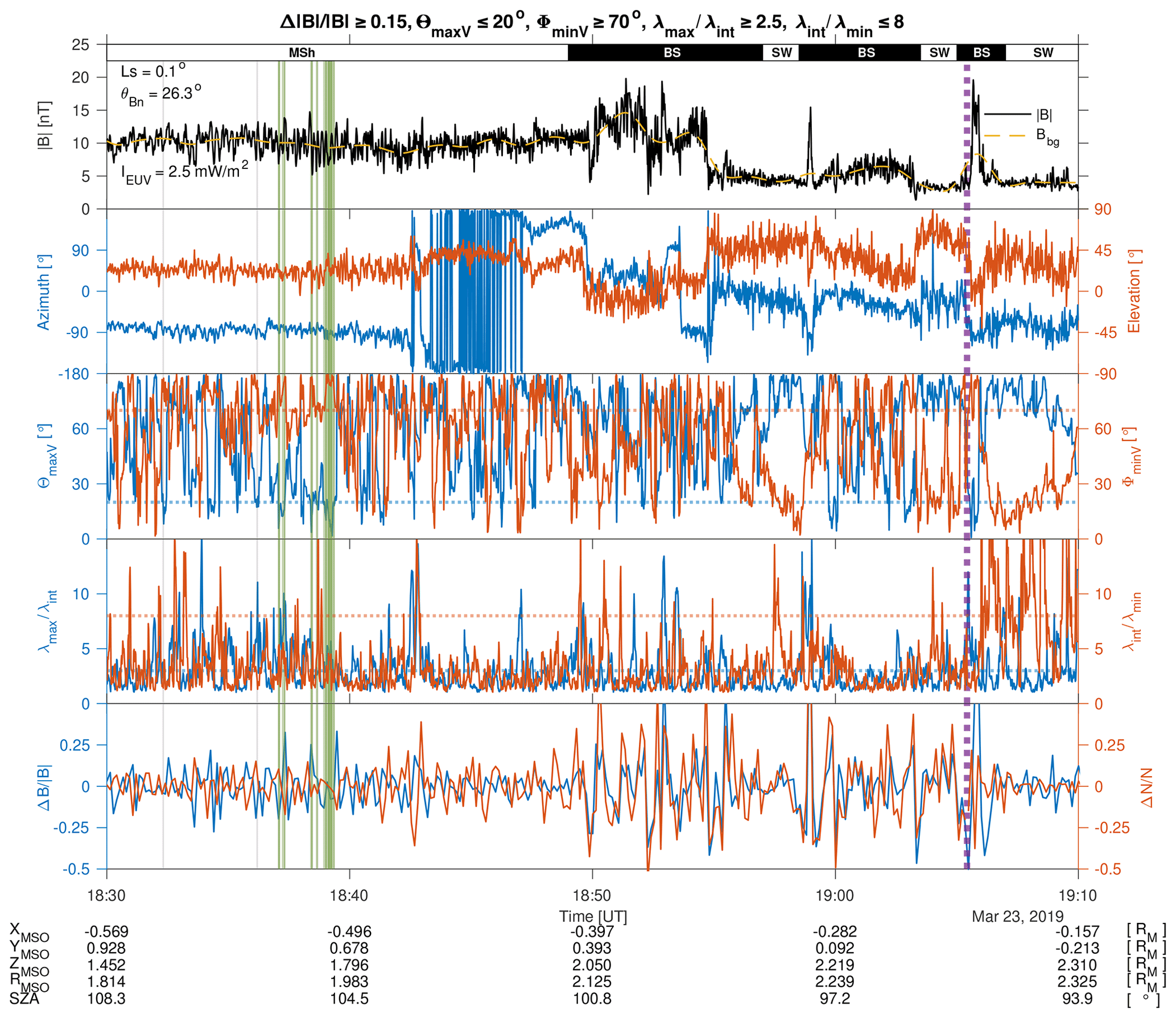
Figure 2Example of MM-like detections at Mars, using the B-field-only criteria of Table 1 on 23 March 2019, at relatively low solar activity. Conditions were: , 〈IEUV〉≈2.5 mW m−2 and (reminiscent of Q- bow shock conditions). Ion density moments were calculated with the 8 s SWICA mode in the magnetosheath before 18:54 UT, and with the 4 s SWIFA mode afterwards. Otherwise, same caption as in Fig. 1. To replace this event in MAVEN's timeline of EUV activity and Ls ranges, see second orange dot in Fig. 4.
At this stage and using Criteria 1–4, the total number of detected 1 s duration MM-like events in the 1 November 2014–7 February 2021 MAVEN dataset was 2 046 533. Two examples of B-field-only detections are presented in Fig. 1 (higher solar activity conditions) and Fig. 2 (lower solar activity) as events in green and grey. We will come back to discussing them in Sect. 2.2.3.
2.2.2 Removal of false positive detections
The detection criteria 1–4 of Table 1 may not exclude structures which may closely resemble MMs but, in effect, are not.
Some structures, appearing as highly compressional, can be generated upstream of and in and around the bow shock surface; they testify to the variability and complex structure of the Martian shock. These non-MM structures include upstream waves such as proton cyclotron waves (PCWs) and ULF foreshock waves (see Mazelle et al., 2004; Romanelli et al., 2013, 2016; Dubinin and Fraenz, 2016; Romeo et al., 2021; Jarvinen et al., 2022, for observations and simulations). Because PCWs are linked to pickup ion processes, they are usually observed at Mars when the exosphere is particularly extended and neutral hydrogen densities significantly increase, that is, around (just after perihelion, ) and during the dust storm season for Ls=[135–225∘] (Mazelle et al., 2004; Romanelli et al., 2016; Halekas et al., 2020; Romeo et al., 2021), in the whole upstream region. PCWs are non-compressive in nature, which is ruled out by Criteria 1–2. Foreshock waves, on the other hand, are linked to back-streaming ions in the quasi-parallel shock. Both types of upstream waves are generated with a circular polarisation, characteristics which are filtered out by our Criteria 3–4 ensuring quasi-linear polarisation. However, due to relative phase velocities with respect to the solar wind plasma, they may become steepened in the vicinity of the shock (see Tsurutani et al., 1987; Shan et al., 2020, for comets and Mars, respectively), their nonlinear growth stage tending towards more elliptical and quasi-linear polarisations, and with a rotation of the magnetic field across the structure in the steepened edge of the structure (Tsurutani et al., 1987; Tsurutani, 1991; Tsurutani et al., 1999; Mazelle et al., 2004; Shan et al., 2020). These nonlinearly evolved waves may sometimes be captured as MM-like by our B-field-only detection Criteria 1–4.
Other types of structures, such as the so-called “fast-mode” type waves, can have similar compressional and polarisation characteristics as MMs; they occur deeper in the magnetosheath and in the magnetosphere. For example, fast-mode magnetosonic waves with quasi-linear polarisations have been observed at Mars downstream of the IMB (Bertucci et al., 2004), in a manner reminiscent of similar waves found downstream of the magnetic pileup boundary at comet 1P/Halley (Mazelle et al., 1989, 1991; Glassmeier et al., 1993), each time with MM waves in B–N antiphase situated just upstream of the boundary. In contrast, the magnetosonic-type waves found by Fowler et al. (2021) close to the ionosphere and generated at the IMB by solar-wind-driven pressure pulses in the foreshock region are usually elliptically polarised. However, as before, certain associated steepened wave packets with strong fluctuations () could also display a more quasi-linear polarisation and be potentially kept as MM-like candidates if we only apply Criteria 1–4 of Table 1.
In all previous cases, magnetic field intensity and plasma density will typically be in phase, as opposed to the expected MM behaviour (Hasegawa, 1969). However, this information is sometimes neither available at the desired (high) time resolution nor practical to derive as in large statistical surveys. We suggest here two mitigation strategies for our B-field-only investigation: (1) making sure that the magnetic field across the structures does not rotate more than about , as theoretically predicted for MMs (Treumann et al., 2004) and in agreement with past observations (Tsurutani et al., 2011), and (2) restricting the detections to magnetosheath conditions only and excluding the region around the bow shock to avoid foreshock transients and upstream waves.
Strategy (1) constrains the detected events to behaviours more reminiscent of MMs: we apply Criterion 5 of Table 1 which ensures that the magnetic field does not rotate significantly across a MM-like structure. From the 1 s magnetic field vector in MSO coordinates, thereby ignoring higher-frequency features which are not at the same scale as the ion-scale candidate mirror-mode structures, magnetic azimuth and elevation angles are defined as
First, within our original database of candidate MM-like detections, we define so-called “detection periods” containing all events consecutively detected, with two periods separated by a minimum of 30 s between one another. We discard periods of isolated singular events, defined as a detected event lasting no more than 1 s within a period. In this way, some of these discarded isolated events (DIEs) are not part of the usual quasi-periodic train of MM structures, which would result in more than one detection within a period. They are instead more reminiscent of the so-called “linear magnetic holes” (LMHs), in the original definition of Turner et al. (1977), structures that we wish to filter out from the database. In contrast, if multiple detections occur consecutively within a whole period, these events may represent in reality either a large MM-like structure or a train of shorter MM-like structures, depending on the length of the period they belong to. The particular value of 30 s between detection periods was chosen empirically as double the length of the longest MM structures found at Mars or Venus (see, for example Simon Wedlund et al., 2022b; Volwerk et al., 2008, 2016). We then estimate how much azimuth and elevation angles fluctuate at the detected position of the candidate event by calculating their running standard deviation 〈σ(az,el)〉 over a 2 min sliding interval, keeping only those events where 〈σ(az,el)〉 is less than 10∘ for each angle (see Lucek et al., 1999; Simon Wedlund et al., 2022b).
Complementarily, strategy (2) may make use of the position of the bow shock crossing in the spacecraft data and ignore the detected events in a range of radial distances around it (or equivalently, in a range of durations around the time of the crossing). For this part, we use the automatic bow shock detection technique explained in Simon Wedlund et al. (2022a), who used a predictor–corrector algorithm based on magnetic field measurements only at Mars. Their list of automatically detected crossings is freely available (Simon Wedlund et al., 2021). It discriminates between (i) crossings from the solar wind into the magnetosheath and from the magnetosheath into the solar wind and (ii) quasi-perpendicular (noted “Q-⟂” in the following) and quasi-parallel (noted “Q-') bow shock crossings. The latter aspect is useful for investigating how the shock configuration impacts the spatial distribution of MM-like structures (see Sect. 2.3). It is important to note here that the technique of Simon Wedlund et al. (2022a) is biased towards the detection of Q-⟂ crossings as it is based on the classic B-field signature of the Q-⟂ shock, with clearly defined foot, ramp and overshoot. Between 2014 and 2021 of MAVEN operations, Simon Wedlund et al. (2022a) recorded a total of 11 967 Q-⟂ and 2962 Q-∥ “clear” crossings, discarding 1,615 crossings where the shock signatures were difficult to automatically ascertain. In addition, knowing where the shock is can be used to automatically ensure that the structures are located in the magnetosheath. In turn, this naturally fulfils Criterion 6 in Table 1, where the background magnetic field Bbg needs to be 2 times higher than the average, but highly variable, interplanetary magnetic field Bimf.
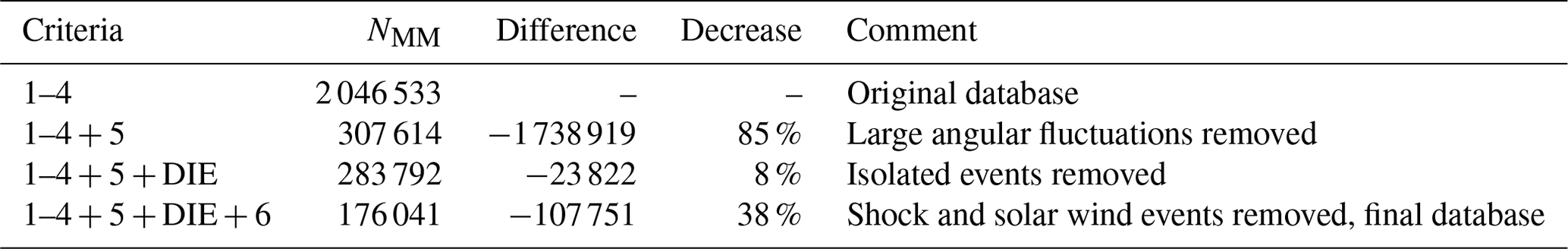
Table 2Total numbers of MM-like events NMM detected at Mars, according to the criteria of Table 1, incrementally, from 1 November 2014 to 7 February 2021 with the MAVEN/MAG instrument. DIE means discarding of isolated events. The most drastic decrease in NMM occurs when including the criterion on magnetic field azimuth and elevation angles, which should not change across a given event by more than 10∘ (Criterion 5).
In practice, knowing when the bow shock crossing took place, we first identify in spacecraft ephemerides the portion of the orbit in the solar wind as opposed to inside the bow shock structure. Then, we remove all MM-like events that are closer than 0.075 RM (∼250 km) to the shock position, assuming that those are shock substructures, situated immediately upstream, at or downstream of the shock itself. This value was chosen empirically from a subset of orbits with magnetic fluctuations that were incorrectly captured by the original detection algorithm (see for an illustration Fig. 1).
Table 2 displays the number of MM-like events detected when incrementally applying the criteria of Table 1, together with the two mitigation strategies discussed above. From the original MM-like events detected in Sect. 2.2.1, strategy 1 (using Criteria 5 and ignoring 23 822 isolated events) removed 85 % of the total number of events: we end up with only 283 792 MM-like detections. Criterion 5 is the criterion that removes most of those events due to the harsh constraint on the stability of the magnetic field angular fluctuations within trains of MM-like events. It shows moreover that Criterion 5 is of utmost importance to remove from the database candidates that are not linearly polarised. Applying strategy 2 to filter out shock substructures and solar wind magnetic holes (based on Criteria 6 and an automatic estimate of the position of the shock) removes another 107 751 events, resulting in a total of 176 041 MM-like events in our final database.
2.2.3 Examples and caveats of the method
Figure 1 (high solar activity conditions) and Fig. 2 (low solar activity) show examples of MM-like detections, with total magnetic field and Criteria 1–4 of Table 1. Detections matching Criteria 1–4 in coincidence are shown as vertical grey and green lines, with the green lines marking the final detections with the removal of false positives (Criteria 1–4 and 5–6 in coincidence).
The events of 8 September 2016 (Fig. 1) occur at and in the wake of a predominantly Q-⟂ bow shock crossing, with angle θBn between the normal to the shock surface and the average interplanetary magnetic field (IMF) direction of about 80∘. Comparison of magnetic field and density variations is displayed in the bottom panel, with magnetic field (left axis, blue) and density (right axis, red) fluctuations being in antiphase when and have opposite signs. For the detections in grey in the ramp of the shock as initially captured by Criteria 1–4 but without removal of false positives, B and N appear mostly in phase at the cruder resolution of the SWIA instrument (here 8 s, with and having most of the time the same sign in the bottom panel). Together with the position within the shock ramp, this implies a false positive detection: further applying Criteria 5–6, they are correctly removed from the final database, leaving only the events in green. The events in green display a mix of B–N in-phase and antiphase behaviours (bottom panel), with some of the shorter detected events appearing in phase, a characteristic more reminiscent of fast mode-type (e.g. magnetosonic) waves; this is however difficult to unambiguously ascertain owing to SWIA's 8 s resolution which cannot capture these shorter magnetic field structures. Around 00:19:30 UT, some oscillations are clearly in antiphase, whereas before and after they seem to become in phase again. Closer to 00:30 UT, B–N fluctuations appear again in antiphase but are not captured by the detection algorithm, due to constraints on the linearity of the structures. This points further to the necessity of a more in-depth case study as in Simon Wedlund et al. (2022b) to ascertain the nature of the fluctuations captured by our algorithm and shows the limitations of a B-field-only algorithm to detect MM structures. From a general point of view, the temperature anisotropies responsible for the generation of MMs are expected to take place in the wake of a Q-⟂ shock (see Hoilijoki et al., 2016). Consequently, we expect such time series, together with those discussed in Simon Wedlund et al. (2022b) (24 December 2014 around 11:25 UT, also at high solar activity) or Ruhunusiri et al. (2015) (26 December 2014 around 15:00 UT in their Fig. 1), to harbour “textbook” examples of MM occurrences.
In Fig. 2 (23 March 2019), detections occur in the solar wind region around 19:15 UT (not shown) and in the magnetosheath towards the IMB around 18:38 UT, behind a predominantly Q- shock (, noted “Q-” in the following). Multiple crossings of the shock from the magnetosheath into the solar wind take place. The automatic estimate of the shock's location following Simon Wedlund et al. (2022a) pinpoints the last great magnetic field enhancement around 19:05 UT, whereas the magnetosheath-to-solar wind position is visually closer to 18:52 UT: this is due to the fact that automatic estimate choosing the last occurrence of a shock-like structure when crossing from the magnetosheath to the solar wind. In the solar wind after 19:05 UT, magnetic field and density seem mostly in phase: two “linear magnetic hole” (LMH) candidates (not shown) are first captured by Criteria 1–4. After they are removed from the database using Criteria 5–6, only MM-like events which are roughly in B–N antiphase (around 18:39 UT) are kept.
That said, other events deeper in the magnetosheath (around 18:33 and 18:36 UT) and part of the database in grey are also removed because they are isolated events: the second of these events around 18:36 UT presents a clear B–N anticorrelation. This shows that although the detection method using Criteria 1–6 appears quite apt at detecting regions where MM-like events are present and at removing events that are clearly not MMs, it may also ignore promising candidates (especially around 18:30–18:34 UT). Conversely, as already mentioned in Fig. 2, we expect the method to also keep events that are likely not MMs although situated in the magnetosheath but with B and N in phase. For illustration, isolated 1 s events, discarded in the final database, amount to 23 822 additional events, which make about 14 % of the final total number of events (see Table 2). As a consequence, on this criterion only (isolated event), we estimate that the frequency of true MM-like detections in our final database could be underestimated by about 10 %.
Another aspect is that several individual structures as part of trains of MMs are likely to have been missed by our B-field-only method; see, for example, in Fig. 2, around 18:35 UT where clear B–N anticorrelations are not captured even by the original detection method. This is an inherent caveat of any automatic detection method based on somewhat arbitrary thresholds and a possibly flawed estimate of the background field (see Joy et al., 2006, who used upper and lower quartiles of B to overcome some of this difficulty). Choosing laxer detection criteria would increase the likelihood of capturing such structures; however this would also be at the expense of increasing false positive detections.
Finally, we only consider in our study so-called “linear” MM-like structures; theoretically, single MMs are purely growing modes, which an elliptical polarisation would prevent. However, as shown in studies made in the Earth's magnetosheath (Génot et al., 2001, 2009), MMs can also be elliptically polarised in certain conditions. A discrimination between all polarisations states is difficult to achieve with B-field-only criteria and is outside of the scope of our study. Therefore, our method may miss a certain (but difficult to estimate) amount of structures which are MMs but are non-linearly polarised in nature.
Several tests have been made on reduced datasets to find the sweet spot of all criteria gathered in Table 1 (see also the discussion in Simon Wedlund et al., 2022b) to keep as many confirmed MM-like structures as possible whilst avoiding other compressional structures that are not MMs. This points overall to the difficulty of characterising such structures reliably with magnetometer-only data. In all cases, after applying our mitigation strategies, the number of events that are captured is thus most likely a lower estimate of the frequency of linearly and non-linearly polarised MM-like structures present around Mars. As shown in Figs. 1 and 2, one way to mitigate these aspects is to check for the antiphase behaviour between B and N (at 4–8 s resolution), at the expense of the smaller MM-like structures. This is outside the scope of our current work which aims at evaluating the B-field-only method of detection; using the full plasma instrumentation on board MAVEN is thus left to a future study, in a way similar to the recent study of Jin et al. (2022).
2.3 Mapping technique
Calculating MM-like occurrence probabilities and mapping them in the magnetosheath of Mars proceed as follows.
2.3.1 Detection probability
First, we apply the B-field-only criteria of Table 1 in coincidence to the whole MAVEN dataset, from November 2014 to February 2021. This yields the timing and duration of MM-like structures, noted tstruct and ΔTstruct, respectively. It is important to remark here that a full dip or peak of any given MM-like structure is usually longer than the total sum of 1 s detections for that structure. This arises from the fact that all the criteria of Table 1 must be simultaneously met to validate this as a detection. Consequently, ΔTstruct can only be an underestimate of the total duration of a structure. Following Simon Wedlund et al. (2022b), we evaluate such an underestimate to at least 50 %, based on visual comparisons in the subset of events presented in Fig. 1, Fig. 2 and in Simon Wedlund et al. (2022b), who, with the same detection algorithm, captured 33 s out of a total of 77 s of visually identified MM structures.
Second, we define a spatial grid for the data accumulation. We start with spacecraft coordinates expressed in the Mars Solar Orbital (MSO) coordinate system (sometimes called “Sun-state” coordinates), where the XMSO axis points towards the Sun from the centre of Mars, and ZMSO points towards Mars' north pole and is perpendicular to the orbital plane defined as the XMSO–YMSO plane passing through the centre of Mars, with YMSO completing the right-hand triad. We then transform this system into aberrated MSO coordinates by rotating the XMSO–YMSO plane 4∘ anticlockwise around the ZMSO axis in order to account for the apparent “aberration” of the orbital motion of Mars with respect to the average direction of the solar wind (Simon Wedlund et al., 2022a). The new aberrated coordinate system, aligned with the average apparent solar wind direction, is noted , and (although by construction). For brevity, the () direction is sometimes referred to as “subsolar” (“antisolar”) direction in the following, although, strictly speaking, they should be referred to as “subsolar-wind” and “antisolar-wind” directions.
A two-dimensional cylindrical coordinate grid can then be created, with the abscissa i along the axis and the ordinate j defined as . The grid resolution is chosen so that, on average, the residence time of the spacecraft in each grid cell is large enough in all cells covered by the spacecraft's orbit. For example, for Mars (average planetary radius RM=3389.5 km) and applied to MAVEN 2014–2021 ephemerides, a resolution of ΔR=0.05 RM ensures that the spacecraft residence time in each (i,j) cell is of the order of 500–1000 s (8–16 min) per grid cell for a typical Mars year of 687 Earth days; for a resolution of ΔR=0.1 RM, average residence times are of the order of 5×10⁴ s (∼ 14 h). The latter resolution of ΔR=0.1 RM is thus chosen to maximise the statistical significance of the MM-like detections. Examples of spacecraft residence times with this grid resolution are shown in Fig. 8, left panels, for several consecutive Mars years.
We can now define the probability 𝒫 of detecting MM-like events in a chosen spatial grid cell (i,j) as the total duration of the detected events ΔTstruct divided by the accumulated residence time of the spacecraft ΔTsc (see also Volwerk et al., 2016):
with k being the number of events found in each grid cell (i,j). In other words, 𝒫 represents the percentage of observations containing a MM-like event at any given point in the magnetosheath. The accumulation of the events in the grid, including those crossing a cell boundary, is naturally taken into account using a bi-variate histogram accumulation.
An example of spacecraft residence time and MM-like detection probabilities is shown in Fig. 3a, b. Figure 3 is discussed further in Sect. 3.1. As mentioned above, because ΔTstruct is an underestimate of the total duration of MM-like structures in the magnetometer dataset, 𝒫 is also underestimated: we thus refer to it as a “detection probability” of detecting MM-like structures.
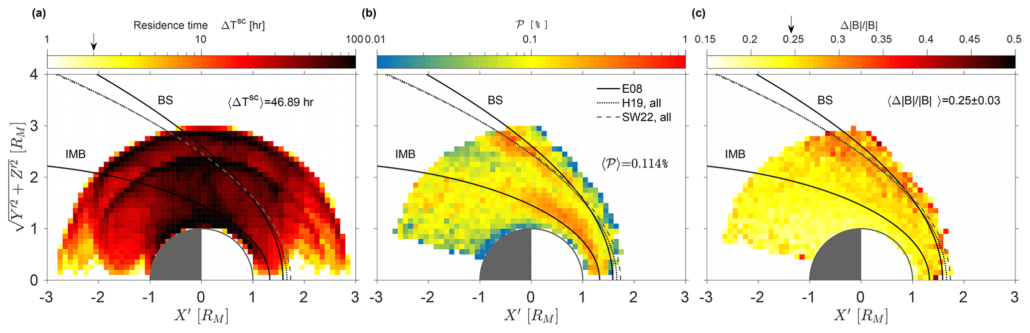
Figure 3Mission-wide results at Mars as observed by the MAVEN/MAG instrument from MY32 to MY35 (1 November 2014 to 7 February 2021). (a) Spacecraft residence time ΔTsc. (b) Percentage occurrence of detecting MM-like structures 𝒫, for ΔTsc≥2 h in any given grid cell. (c) Magnetic field fluctuations . In panel (c), the mean magnetic fluctuation of 0.25±0.03 is highlighted by an arrow on the colour bar. In panel (a), the average residence time in a grid cell 0.1×0.1RM, noted 〈ΔTsc〉 is given for reference. In panel (b), the average probability 〈𝒫〉 in a grid cell, ignoring all grid cells for which ΔTsc<2 h (vertical arrow in the colour bar of panel a), is also given. The average positions of the “nominal” bow shock (BS) and of the induced magnetospheric boundary (IMB) are given for reference as black continuous lines (Edberg et al., 2008, noted “E08”), based on MGS data. Other bow shock positions representative of Mars Express and MAVEN datasets are in dotted lines (Hall et al., 2019, all points, noted “H19”) and as dashed lines (Simon Wedlund et al., 2022a, all points, noted “SW22”). The average IMB and the BS lines roughly delimit the magnetosheath region; of note, detections seemingly outside of this average bow shock on the picture are in reality always inside the shock for individual events. Coordinates are solar wind-aberrated, normalised to the radius of Mars (RM=3389.5 km).
2.3.2 Characterisation with respect to physical parameters
To study how the distribution of MM-like structures varies during the time of the mission, we choose several controlling physical parameters, which are summarised in Fig. 4. We discriminate our results against the following.
-
Mars Year (MY): on average, one MY lasts 1.88 Earth years (687 Earth days). Because MAVEN started its scientific investigation in November 2014, we consider data from this date (after the autumn equinox of MY32) up to MY35 (ending on 7 February 2021). Precise start and end times for each MY were obtained from the equation of time of Allison and McEwen (2000) (their Eq. 14). For reference, MY32 = [31 January 2013–18 June 2015 12:34 UT], MY33 = [18 June 2015 12:34 UT–5 May 2017 11:45 UT], MY34 = [5 May 2017 11:45 UT–23 March 2019 11:32 UT] and MY35 = [23 March 2019 11:32 UT–7 February 2021 11:12 UT].
-
EUV flux levels: following Halekas et al. (2017b) and Gruesbeck et al. (2018), we use two EUV flux levels: one “high” for EUV fluxes IEUV≥0.00277 W m−2 and one “low” for fluxes IEUV<0.00277 W m−2. This limit, noted 〈I〉 in the following, is the median of the EUV flux in the 2014–2021 period as calculated from FISM-IUVS' daily irradiance at 121.5 nm (Lyman-α line), itself derived from the Mars EUVM model (Thiemann et al., 2017). It is also close to the threshold value of = 0.0029 W m−2 considered by Gruesbeck et al. (2018) for the first year of MAVEN observations. During the time of the mission, the solar activity went from medium to low (from MY32 to MY34) followed by a slight recovery during MY35; local peaks in the measured EUV flux correspond to perihelion conditions and local dips to aphelion conditions (see Fig. 4).
-
Solar longitude (Ls): Ls measures the position of a planet in its orbit around the Sun. Because Mars has a relatively high orbital eccentricity (ϵ=0.0935) and is tilted 25.2∘ with respect to its orbital plane, Ls is also a measure of atmospheric seasons. (, respectively) corresponds to perihelion (aphelion) conditions. In this study, we use four ranges centred on equinoxes and solstices: Ls1 = [315–45∘] (northern hemisphere [NH] spring equinox), Ls2= [45–135∘] (NH summer solstice), Ls3= [135–225∘] (NH autumn equinox), Ls4= [225–315∘] (NH winter solstice). Season timings were also obtained from Allison and McEwen (2000) (their Eqs. 15–19). See Fig. 4 for the centred seasons with respect to time.
As discussed in Halekas et al. (2017b) and Simon Wedlund et al. (2022a), each controlling parameter is co-dependent on other parameters. The Martian atmosphere depends on a complex interplay between heliocentric distance, axial tilt and atmospheric circulation (Dong et al., 2015). At perihelion (), the solar EUV flux is largest (see Fig. 4) and causes the Martian exosphere to progressively heat up and significantly expand (Forbes et al., 2008). In their study of the hydrogen (H) exosphere's seasonal variability, Halekas (2017), confirmed by Halekas and McFadden (2021), found a peak of H column density around the NH winter solstice (), suggesting either a degree of latency in the exosphere's response to solar inputs, a seasonal component due to lower atmosphere dynamics or both. Simultaneously to these complex changes, increased EUV fluxes lead to increased ionisation in the ionosphere and in the exosphere far in the upstream solar wind (increased charge exchange and pickup ion process), leading to the induced magnetospheric obstacle to the solar wind to grow in size (Hall et al., 2016, 2019). Consequently, one Ls bin (representing a Martian season) encompasses effects arising from several mechanisms affecting the extent of the exosphere and that of the Mars plasma environment (Yamauchi et al., 2015): global atmospheric circulation, presence of dust storms or EUV inputs, themselves a function of heliocentric distance and solar cycle (Trainer et al., 2019). Similarly, any given Mars year includes variations in atmospheric seasons and EUV flux (since the solar EUV flux varies significantly with heliocentric distance, to which the solar activity variations are superimposed). Either Mars years, Ls or EUV flux levels indiscriminately contain all bow shock geometries, Q- or Q-⟂ alike.
For each of the above controlling parameters, external drivers include the highly variable solar wind inputs, such as dynamic pressure and Mach number (Halekas et al., 2017b). This makes it all the more difficult in practice to isolate the role of a single controlling parameter from the others. For example, one way to help disentangle these effects would be to study the seasonal changes at a fixed EUV flux level or, inversely, to study a EUV flux level at a fixed seasonal bin. However, depending on the chosen binning, the event statistics may become too low for a statistically significant interpretation. We leave this for a future study, when MAVEN will have completed several additional MYs, and choose a complementary approach using the probability density function (PDF) of the total number of detected events as a guide (see Sect. 3.2.1).
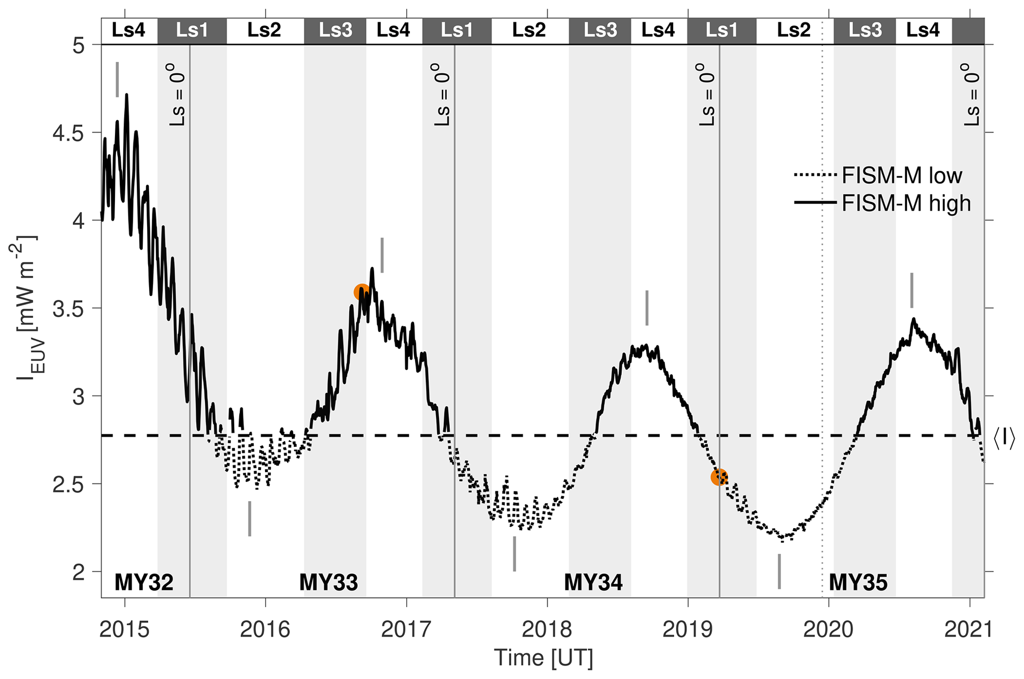
Figure 4Lyman-α daily modelled irradiance levels IEUV between MY32 and MY35 as derived from the EUVM instrument on board MAVEN and corrected with the FISM-M EUVM model (Thiemann et al., 2017). The median of the irradiance throughout this period 〈I〉 is 2.77 mW m−2 (horizontal dashed line) which separates in our study high EUV conditions from low EUV conditions at Mars. Mars years (MYs) and northern hemisphere seasons (Ls) are highlighted, with marking the northern spring equinox and the start of a new Mars Year. Here, Ls1=[315–45∘], Ls2=[45–135∘], Ls3=[135–225∘] and Ls4=[225–315∘] for brevity. The timings of aphelia (local minima of IEUV, ) and perihelia (local maxima, ) are indicated as short vertical grey lines. Solar cycle 25 started in December 2019, marked as a vertical dotted line. The orange dots correspond to the timings of the two examples presented in Figs. 1 and 2.
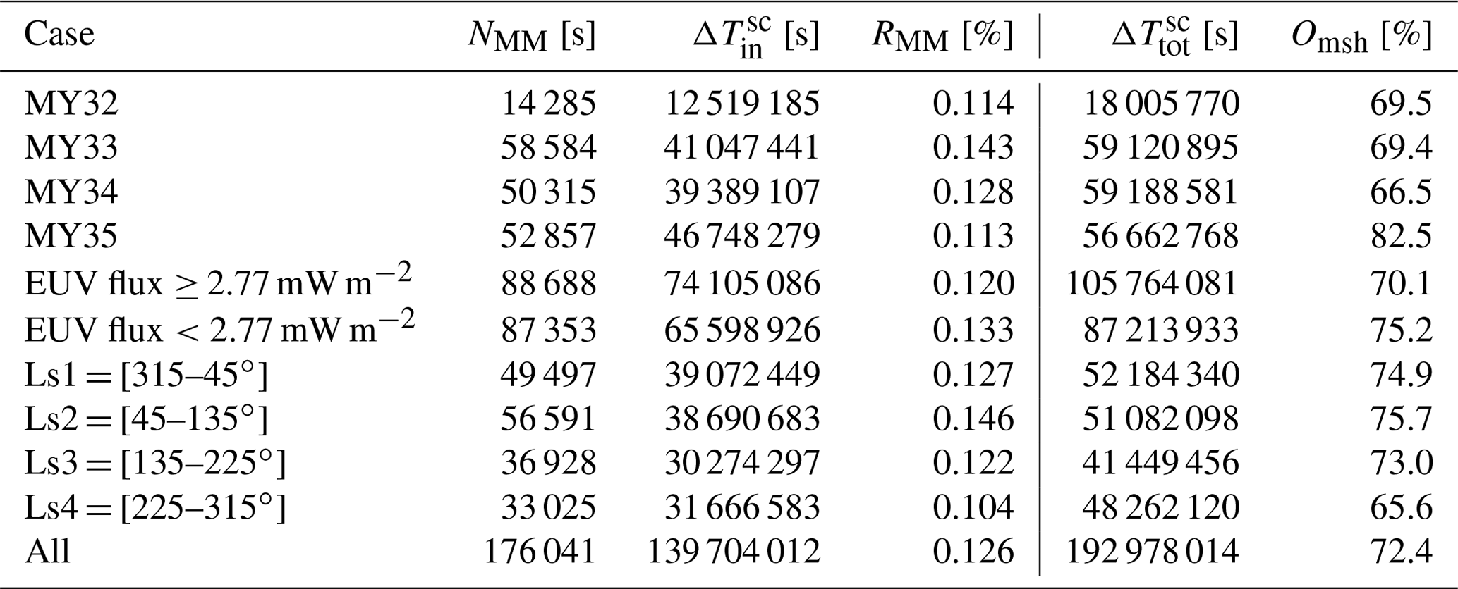
Table 3 presents the general statistics of our MM-like structure database, with a total of 176 041 events detected between 1 November 2014 and 7 February 2021 (last day of MY35), with a total residence time of the spacecraft in the magnetosheath and magnetosphere of about 4.4 Earth years, compared to a total orbiting time of 6.1 Earth years. For each controlling parameter we calculate the residence time of MAVEN inside the bow shock of Mars and the global observation ratio of MM-like events. By contrast, we also calculate the total residence time of MAVEN and the proportion in percentage that MAVEN spends inside the bow shock during its orbiting time around Mars, using the fast bow shock detection of Simon Wedlund et al. (2022a) to pinpoint where the magnetosheath finishes and the solar wind starts in the individual orbits. During the time span covered, MAVEN remains about 70 % of its orbiting time downstream of the bow shock. In Sect. 3, we will discuss the significance of these ratios and contrast them against the detection probability maps.
Table 3Statistics of MM-like event in the magnetosheath of Mars found from 1 November 2014 to 7 February 2021 with the MAVEN/MAG instrument, following the detections performed in Sect. 2.2 and for different cases. NMM represents the total number of MM-like events found (equivalent to a duration in s because of the magnetometer resolution of 1 s). is the total duration that the spacecraft spent inside the bow shock of Mars during that time (excluding thus the time spent in the solar wind), whereas is the total time spent by MAVEN in the whole volume of space, given here as a comparison. Observation ratio is the percentage of MM-like detections in the magnetosheath, and is the proportion of the full orbit coverage that MAVEN effectively spends in the magnetosheath; both are expressed in percentages.
We now present the statistics and the 2D cylindrical coordinate occurrence maps of MM-like structures in the magnetosheath of Mars resulting from our automatic detections described in Sect. 2.2 and 2.3.
3.1 Overview of the full dataset
Figure 5 shows the probability density function (PDF) of several characteristic quantities for the 176,041 MM-like events detected from 1 November 2014 to 7 February 2021 (MY32 to MY35): magnetic field intensity (panel a) as well as those of Criteria 1–4 inside the structures (panels b to f). For each, we indicate the bin position of the peak of the distribution. Most detected events exhibit characteristics that are close to the criteria threshold values (panels b, c and e). The eigenvalue ratios extracted from the MVA (panels e and f) show that the variance ellipsoid is cigar-shaped, although not exceedingly so, with most values having λmax≥2.5λint and λint≥1.6λmin. The variance ellipsoid is also oriented along the average background magnetic field direction, as shown in panels (c) and (d), with most values having ΘmaxV≲18 and . Together, these criteria make sure that the structures are highly compressional and quasi-linearly polarised, as expected from MMs.
The spatial distribution of the detected structures is shown in Fig. 3 as maps for the full dataset considered here, with a bin resolution of 0.1 RM. For reference, we also indicate the “nominal” bow shock (BS) and induced magnetospheric boundary (IMB, sometimes referred to as “magnetic pileup boundary”) from several previous studies (Edberg et al., 2008; Hall et al., 2019; Simon Wedlund et al., 2022a). Because these boundary positions were determined statistically and represent an average over an extensive range of geophysical conditions, their exact position may vary by a few grid cells for individual observations and should only be taken as a rough indicator of the shape of the boundaries around that point. Figure 3a displays the residence time of the spacecraft ΔTsc: on average, MAVEN spends a little less than 47 h in each cell with a very homogeneous coverage throughout, except in the subsolar region in the upstream solar wind and in the deep magnetospheric tail in the antisolar-wind direction. The regions of maximum orbital coverage are close to the IMB and around the terminator plane in the magnetosheath.
The spacecraft residence time ΔTsc is then used as a normalising factor to calculate the probability 𝒫 of detecting MM-like events (Fig. 3b), expressed here in percentage and in logarithmic scale. In this representation, we ignore all grid cells for which ΔTsc<2 h to ensure a good statistics: MAVEN thus stays a minimum cumulated time in each cell equivalent to about 250 times the duration of the longest single MM-like structure at Mars (∼ 30 s).
MM-like structures are mostly confined to two main regions: one in the immediate vicinity of the predicted shock (at ) and one in the magnetosheath pressed against the IMB. Both of these regions have 𝒫>0.2 % with maximum values of 0.5 %–0.8 % reached in the subsolar region of the magnetosheath, close to the IMB. A third region can be identified in the magnetospheric tail, where occasional high probabilities are encountered. Qualitatively, this is very similar to the results of Ruhunusiri et al. (2015), who showed that MM waves were predominantly present in MAVEN's first year of operations in the deep magnetosheath and in the tail. They reported average occurrence ratios of less than 10 % somewhat uniformly distributed in the volume of space, with peaks between 10 % and 25 % occurring in three main regions: the middle of the magnetosheath for , closer to the IMB for and in the magnetospheric tail inside the statistical IMB. Although our main detection regions are similar to those of Ruhunusiri et al. (2015), both in position and shape, we report here much lower absolute detection probabilities of MM-like events (maximum of 0.8 %). If we take into account the length of the datasets considered in each study, their results included about 4 months of observation during MY32 and thus are most comparable to our Fig. 8a. However, a quantitative comparison with the values of Ruhunusiri et al. (2015) appears extremely challenging at this stage. One reason is that the two detection methods are fundamentally different: ours uses a B-field-only 1 s resolution at the expense of an ambiguity in the nature of the detected structure with a clear underestimate of the total duration of the found events, whereas theirs uses wave analysis techniques based on transport ratios with a cruder time resolution (4–8 s with a Fourier transform on consecutive 128 s intervals), looking for the mode producing the maximum of B-field power in each 128 s window. In that way, our quantitative results are more comparable to those of Jin et al. (2022), who recently found, with similar techniques as ours (but using the additional B–N antiphase behaviour), an occurrence rate of less than 2 % on average over the first 4 years of MAVEN data. The strategies we applied to help remove possible false positive detections may, to a certain extent, have filtered out legitimate events. Moreover, as explained in Sect. 2.3.1, the total duration of MM-like events ΔTstruct is underestimated in our approach by more than 50 % because of inherent limitations in the detection method. All points combined, this implies that our detection probability should be seen as a lower estimate (see Sect. 2.2.2).
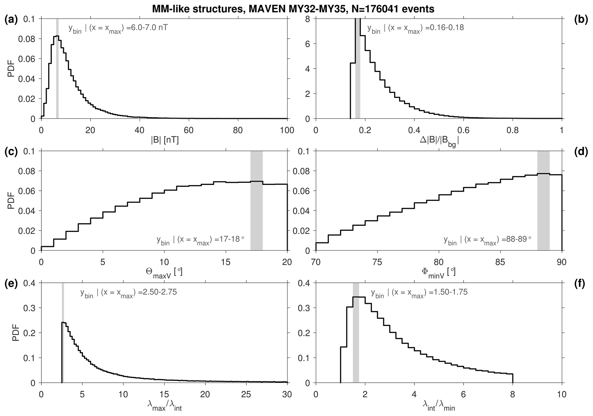
Figure 5Probability density functions (PDF) for the criteria given in Table 1 for the MM-like events detected with MAVEN/MAG from MY32 to MY35 (1 November 2014 to 7 February 2021). (a) Total magnetic field intensity , in bins of 1 nT. (b) Magnetic field fluctuations , in bins of 0.02. Panels (c) and (d): angles between average magnetic field direction and maximum (minimum) variance direction ΘmaxV (ΦminV), in bins of 1∘. Panels (e) and (f): ratios of maximum to intermediate (intermediate to minimum, ) eigenvalues, in bins of 0.25. The position of the maximum of the PDF and its typical bin is marked by a grey zone. All bins are uniformly distributed.
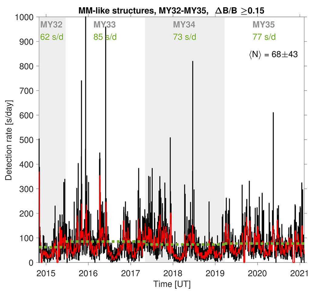
Figure 6Daily detection rate of MM-like events as observed by the MAVEN/MAG instrument from MY32 to MY35 (1 November 2014 to 7 February 2021), using the criteria of Table 1 and considering magnetosheath-only observations. The red line corresponds to the running mean of the black curve over 7 d, and the dotted green line corresponds to Mars Year averages (given as numbers in the top). 〈N〉 is the median of the whole signal in black, with its corresponding standard deviation. Because MAVEN can spend up to 30 % of its time per orbit in the solar wind (see Table 3), all numbers quoted here could tentatively be multiplied by a factor 1.5, with 〈N〉≈100 detections d−1 giving a conservative estimate.
In contrast to the two main high-probability regions discussed above, we identify a region of low probabilities in the portion of the sheath behind the terminator plane and in the tail, where 𝒫<0.1 %. We hypothesise that this is due to the plasma flow configuration which may preferentially transport the MMs almost unchanged from their birth region behind the Q-⟂ shock down to the IMB and along it.
Quantitatively, these results are in line with studies at Venus (Volwerk et al., 2016; Fränz et al., 2017), which registered detection probabilities of less than 5 % on average, with maxima of occurrences taking place immediately behind the shock and close to the IMB. As in our results, these authors also pointed out increased occurrences in the magnetospheric tail. It is important to remark here that the average modelled position of the shock appears in Fig. 3b to fall in the middle of the distribution; however, because we removed shock substructures from the dataset (see Sect. 2.2.2) and considered only magnetosheath events, all of the events shown here are in effect in the magnetosheath and not in the solar wind. This attests to the high variability of the shock position and the limitations of a single modelled curve to represent accurately the position of the shock, a conclusion in conformity with dedicated studies (Gruesbeck et al., 2018).
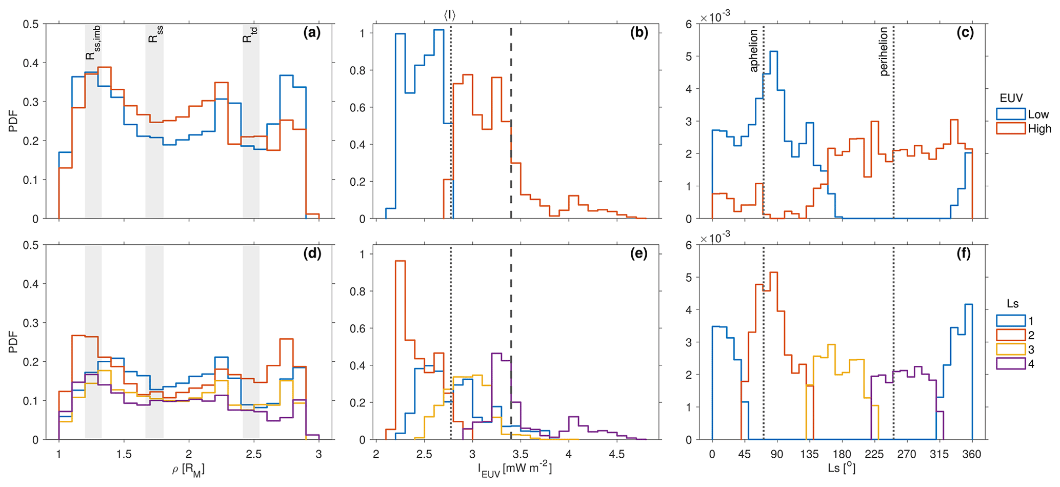
Figure 7Probability density functions (PDFs) of 176,041 MM-like events detected from the end of MY32 to the end of MY35. Panels (a)–(c) discriminate between two irradiance levels, IEUV<2.77 mW m−2 (low EUV flux, blue lines) and IEUV≥2.77 mW m−2 (high EUV flux, red lines). Panels (d)–(f) discriminate between four Ls seasons (Ls1–4), as defined in Fig. 4. These PDFs are calculated for the following parameters: Panels (a) and (d): radial polar coordinate , in bins of 0.1RM. The radius of Mars is RM=3389.5 km; Panels (b) and (e): EUV irradiance IEUV, in bins of 0.1 mW m−2; Panels (c) and (f): seasons (Ls), in bins of 10∘. The PDF is normalised to the total number of detected events, i.e. 176 041. Some remarkable features are pointed out by a vertical dashed line, i.e. transition region in PDF in panels (b) and (e). Moreover, we also include: in panels (a) and (d), the range of positions of the subsolar and terminator standoff bow shock distances Rss and Rtd (Simon Wedlund et al., 2022a, between low and high EUV conditions) and the range of subsolar IMB positions, Rss,imb (Trotignon et al., 2006; Edberg et al., 2009); in panels (b) and (e), the median value of the EUV flux 〈I〉=2.77 mW m−2; in panels (c) and (f), the aphelion () and perihelion positions ().
Magnetic field compressional fluctuations for the detected events are next shown in Fig. 3c. Following Criterion 1, we consider only events with . Fluctuations are comparatively higher in the magnetosheath () and relatively low in the magnetosphere (delimited by the average IMB, with ). More precisely, some of the largest magnetic fluctuations occur close to the terminator plane around the shock and in the subsolar magnetosheath closing in on the IMB, with values often reaching 0.4 and above. Median fluctuations are 0.25±0.03 for the detected events at the chosen grid resolution. In the magnetosphere's tail, certain cell-by-cell fluctuations are quite abrupt from low to high values, in part due to the increasingly poor orbital coverage in this region.
Figure 6 displays the daily detection rate of MM-like detections inside the bow shock during the entire mission. The numbers quoted here represent an accumulation of the detected events in the magnetosheath over a full 24 h of observation by MAVEN. However, during the time span considered here, MAVEN spent at most 30 % of its time in the solar wind per orbit (see Omsh in Table 3), and so all magnetosheath detection rates quoted here should be multiplied by about a factor at least to compensate for the absence of temporal coverage when in the solar wind. For simplicity, we will quote the numbers below as they are, and apply a corrective factor when generalising and comparing to other studies. On average throughout MY32 to MY35 with MAVEN, we find 〈N〉=68 detections per day (ignoring single isolated 1 s events; see Sect. 2.2.2) fulfilling the criteria of Table 1. Because of the MAG resolution chosen, this represents 68 s of detected events per day, or 2.8 detections per hour. Large departures from the 7 d average in red can be seen, but they appear to steadily decline over time. This behaviour coincides with a progressive decline of EUV flux and solar activity at Mars during that period (compare with Fig. 4). For further comparisons, we look at the evolution of this detection rate with respect to MY, assuming that MAVEN's orbit coverage of the magnetosheath was similar between MYs. The latter assumption is mostly fulfilled for MY33 and MY34 (as can be seen later in Fig. 8, left column), with similar orbits and a similar amount of time spent in Mars' environment, whereas MY32, and to a lesser extent MY33, have quite different spatio-temporal coverages. The mean daily detection rate over each MY changes little (dotted green line on the figure), with MY33 having more detections (85 detections d−1 in mostly high EUV flux) than any other year and MY34 (73 detections d−1 in mostly low EUV flux) having less detections. As expected, MY32 seems to be a clear outlier due to a looser coverage around the subsolar magnetosheath and MAVEN probing only the later portion of the full MY. This suggests that we cannot compare absolute detection numbers between MYs without first normalising to the spacecraft's residence time during that period. Such a normalisation is performed and discussed in Sect. 3.2.
Following Madanian et al. (2020) who used MAVEN measurements over a period of 3 months, magnetic holes in the solar wind represent about 2.1 LMHs d−1, lasting about 20 s each, that is, a total of 40–50 s of LMH detection per day. This number can be tentatively compared to our results if we consider that applying Criteria 1–4 only on MAVEN's magnetometer data does not filter out solar wind LMHs from our MM-like event database. In that case, we obtain ∼ 180 s of events per day. Removing the 50 s d−1 of LMHs, we end up with 130 s d−1, a number marginally larger than our corrected (lower) estimate of s of MM-like detections in the magnetosheath (Criteria 1–6). This would be statistically consistent with the hypothesis that the majority of the events captured in the solar wind are isolated events reminiscent of LMHs, as discussed when attempting to remove false positive detections (see Sect. 2.2.2). Conversely, if we assume that a typical MM-like structure lasts about 10 s on average (as in Simon Wedlund et al., 2022b), we end up with 100 s divided by 10 s, i.e. ≈ 10 MMs d−1 in Mars' magnetosheath.
3.2 Spatial dependence on physical parameters
Spatial maps of MM-like structures around Mars detected with MAVEN using magnetic-field measurements are discussed below with respect to the controlling parameters expounded in Sect. 2.3.2. Before examining these in more detail, we present a few considerations based on their probability density function (PDF).
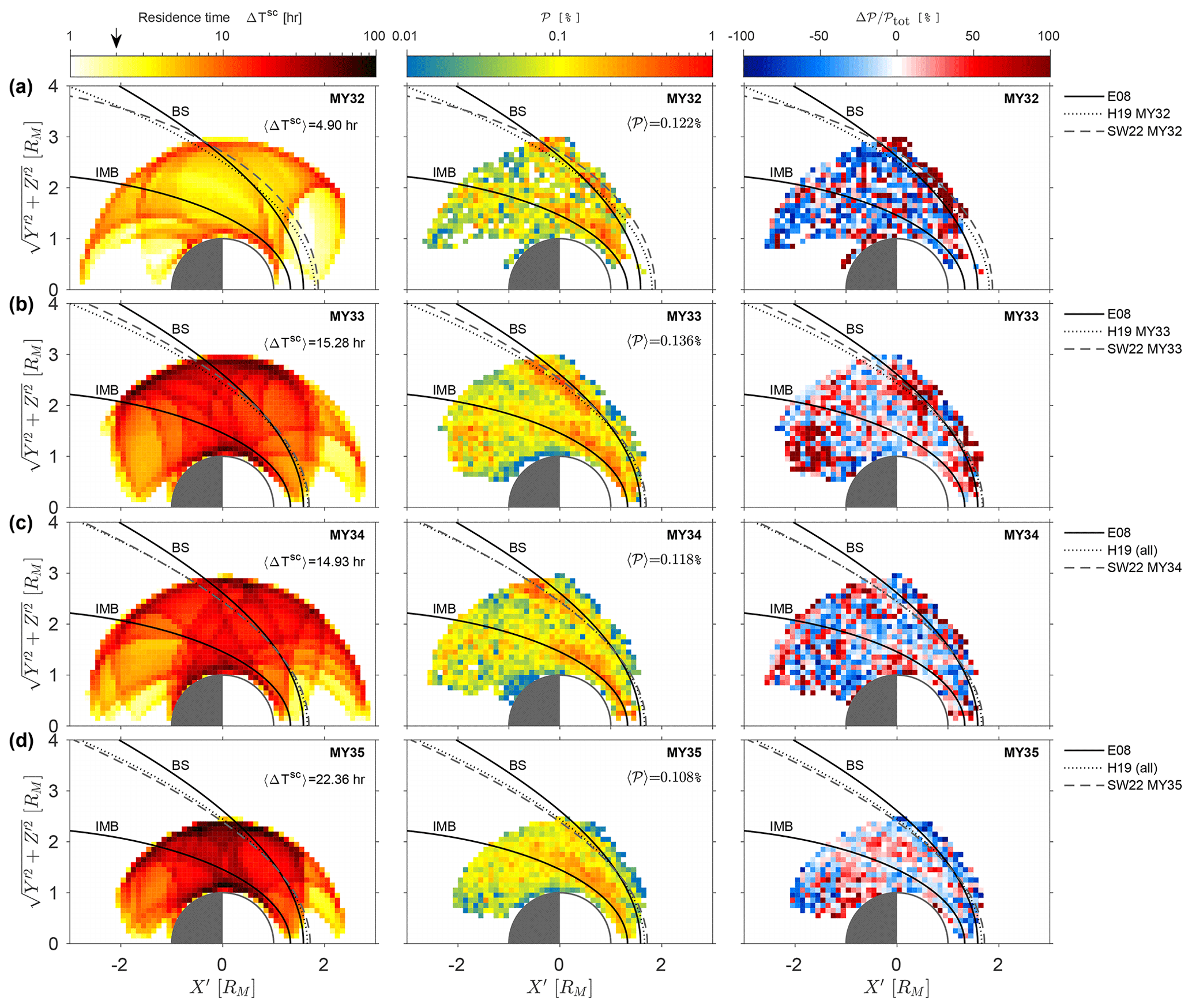
Figure 8Residence time (left), probability 𝒫 of detecting MM-like structures (middle) and departure from the total detection probability (right) at Mars, binned by MY. The percentage difference is calculated as , with positive hot-hued (negative cold-hued) values showing where 𝒫MY>𝒫tot (𝒫MY<𝒫tot). The total rate 𝒫tot is taken from Fig. 3b. B-field data only with MAVEN/MAG were used in the detection, from 1 November 2014 to 7 February 2021. (a) MY32. (b) MY33. (c) MY34. (d) MY35. Bow shock average positions are shown as dotted lines (Hall et al., 2019, MY32, MY33 and all points, noted H19) and in dashed lines (Simon Wedlund et al., 2022a, for each MY, noted SW22). See also caption of Fig. 3 for other details.
3.2.1 Probability density function (PDF)
Figure 7 presents the PDF of the detected MM-like structures with respect to radial polar coordinate (panels a and d, in bins of 0.1 RM which is the resolution of our 2D distribution maps), EUV flux levels (panels b and e, in bins of 0.1 mW m−2) and Ls (panels c and f, in bins of 10∘). Each PDF is discriminated against high and low solar flux levels (panels a–c) and against Ls ranges (panels d–f, with Ls1–4 for NH spring, summer, autumn and winter) to illustrate the co-dependence of the studied parameters. Panels (b) and (f) represent the baseline statistics of IEUV and Ls parameters. They highlight the bins where the PDFs have larger values and hence the parameter has a good statistical coverage. For example, the sharp drop in PDF occurring for IEUV>3.4 mW m−2 in Fig. 7b is due to the smaller spacecraft orbital coverage above this threshold: this is also clearly seen in Fig. 4, where only MY32 and MY33 contribute to the statistics, with the threshold 〈I〉 just above the irradiance local peaks during MY34 and MY35. Successive Ls ranges are in contrast quite homogeneously distributed with relatively constant PDFs throughout (Fig. 7f), with the Ls2 range having the largest PDF overall. Note that in Fig. 7b and f, the finite width of EUV (single precision compared to the double precision IEUV threshold) and Ls bins results in expected overlaps at the borders between blue, red, orange and purple lines.
In Fig. 7a, d, we see a combined peak of the PDFs in the 1.2–1.3 RM bins, close to the position of the IMB (Rss,imb=1.25–1.33 and Rtd,imb∼1.45; see Trotignon et al., 2006; Edberg et al., 2009). The PDF drops by almost half around 1.5 RM, roughly 0.2 RM ahead of the bow shock's variable subsolar position. Hence, a rather homogeneous ring of MM-like structures around the planet forms, centred on 1.2–1.3 RM, as already seen in Fig. 3. Overall, the distributions look very similar for all EUV and Ls ranges considered. However, we see two more prominent peaks of the PDF: one 0.1–0.2 RM inwards of the terminator standoff distance Rtd (true for all EUV conditions and Ls ranges) and the other 0.2 RM outwards of it (low EUV conditions, Ls2 contributing most, Ls4 the least due to reduced spatial coverage of MAVEN in these conditions). These two peaks correspond in Fig. 3 to the tail detections around 2.3 RM from the centre of Mars and to the detection enhancement around the average shock position in the terminator plane around 3 RM.
The co-dependence between EUV flux and Ls range is clearly seen in Fig. 7c and e. Obviously, aphelion and perihelion conditions mostly correspond to PDFs for low and high EUV solar fluxes, respectively. The main peak in the PDF appears in bin Ls=80–90∘ within the “Ls2” range (see also Fig. 7f), slightly after aphelion conditions. No peak in the PDF particularly stands out for and higher EUV fluxes, although a relatively lower PDF seems to occur around perihelion conditions. Complementarily, in Fig. 7f and e, range Ls2 (Ls=45–135∘, containing aphelion conditions) is dominated by low EUV fluxes, whereas Ls4 (Ls=225–315∘, containing perihelion conditions) is dominated by high EUV flux, with the first range strongly peaking at IEUV∼2.3 mW m−2 and the second range at IEUV∼3.3 mW m−2. Consequently, these two Ls ranges appear to be a good proxy of conditions driven by seasons only at an almost constant EUV flux, either low or high. The remaining two Ls ranges, Ls1 (Ls=315–45∘) and Ls3 (Ls=135–225∘), have similar distributions with respect to EUV flux and are thus more comparable to one another.
Overall, these preliminary results are consistent with past observations at Mars, be it with MGS (Bertucci et al., 2004) or with MAVEN (Simon Wedlund et al., 2022b), who all noted that MM structures seemed to pile up against the IMB. This suggests that MMs, after being created upstream of their detection place, are convected down to it with the ambient plasma flow. Using the full MAVEN plasma complement and owing to the ambient plasma becoming less unstable to MMs the further away from the shock, the locus of generation of the MMs found by Simon Wedlund et al. (2022b) was inferred to be in the immediate wake of the Q-⟂ shock, a condition that seems to predominate in the 2014–2021 MAVEN dataset (Simon Wedlund et al., 2022a).
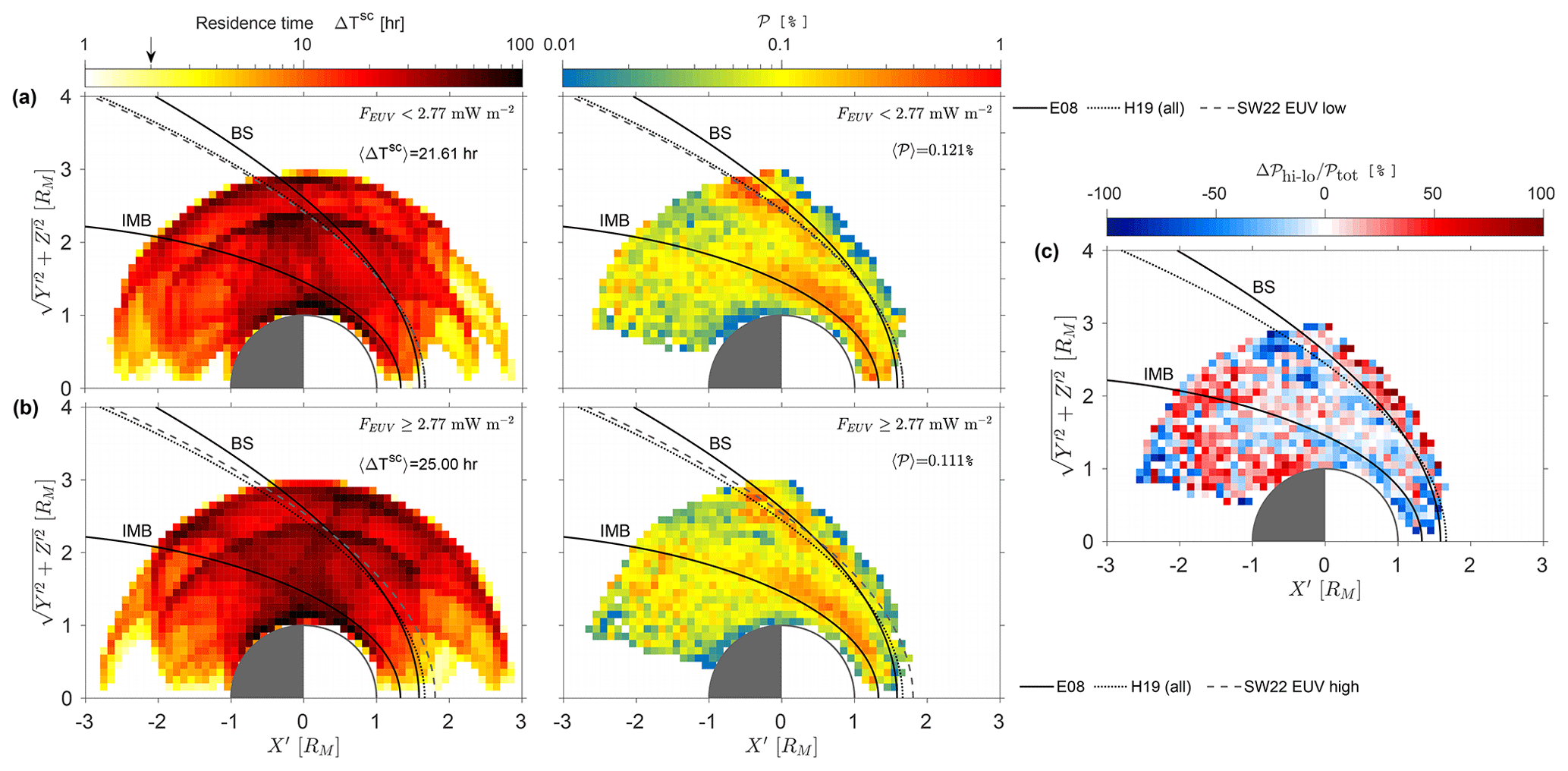
Figure 9Residence time (left) and probability 𝒫 in % of detecting MM-like structures (middle) at Mars, with respect to EUV irradiance levels. (a) Low EUV fluxes. (b) High EUV fluxes. (c) Relative difference between high and low EUV levels with respect to the total detection probability, , expressed in percentage. As before, 𝒫tot is the map obtained in Fig. 3b. The colour yellow indicates regions with the same probabilities between the two conditions, whereas blue “cold” hue (red “hot” hue) regions indicate where 𝒫 is dominated by low (high) EUV conditions. Bow shock average positions are shown as dotted lines (Hall et al., 2019, all points, noted H19) and as dashed lines (Simon Wedlund et al., 2022a, for each EUV flux level, noted SW22). See also caption of Fig. 3 for other details.
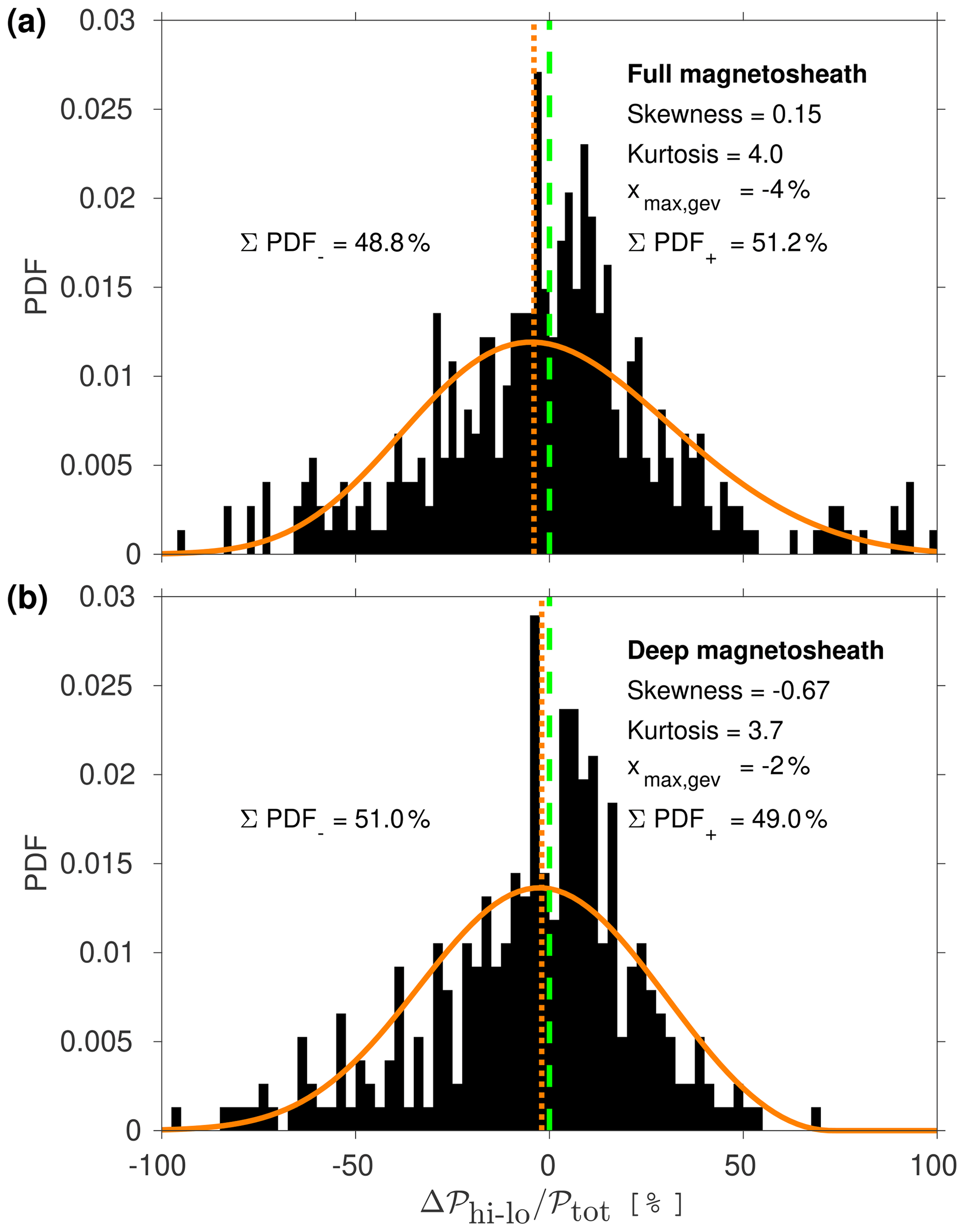
Figure 10Probability density function of EUV-discriminated relative detection probabilities, for the “full magnetosheath” (a), and for the “deep magnetosheath” (b). As in Fig. 9c, we calculate the relative difference between high and low EUV levels with respect to the total detection probability, , expressed in percentage, with positive values showing preponderance towards high EUV conditions, and negative values towards low EUV conditions. “Full magnetosheath” considers the detection probabilities outside of the average IMB (defined by the fit of Edberg et al., 2008, for MGS data at high EUV flux conditions), whereas “Deep magnetosheath” only considers 𝒫 in the narrow region delimited by the two black continuous lines in Fig. 9c, between the two average fits of Edberg et al. (2008). Generalised extreme value (GEV) fits to the distributions are shown in orange, together with their peak position (dotted vertical line). The symmetric position where 𝒫hi=𝒫lo is given as dashed green line. Deviation from a symmetric distribution is given by the skewness of the distributions: negative skewness highlights a distribution whose mass is concentrated on the left (low EUV conditions, ), whereas a positive skewness has the distribution concentrated towards the right (high EUV conditions, ). A kurtosis of more than 3 as calculated here implies that the tails of the distributions are heavier than those of the normal distribution. (respectively, ) represents the percentage of the total PDF that lies on the left (right) of the “zero” dashed green line.
3.2.2 Dependence on Mars Year
Figure 8 presents, for four MYs (panels a–d), the spacecraft residence time (left panels), the MM-like detection probability 𝒫 (middle panels), and their relative difference (right panels) with respect to the total detection probability 𝒫tot (taken from Fig. 3b), in the same format as in Fig. 3. Because MAVEN started observing late in Oct. 2014 (towards the end of MY32), the statistical coverage for MY32 is lower than for MY33–MY35, with a residence time in a grid cell on average about 3 times less than any other year. Similarly, because of the orbit being more compact around the planet during MY35 (panel d), the mean residence time in a given grid cell is significantly higher than for the other years. However, relatively high average residence times above 5 h ensure a good statistical coverage of the spatial plane.
The detection probabilities are shown in percentages on the middle panels, when, as for Fig. 3, all grid cells for which ΔTsc<2 h are discarded to ensure an optimal statistics. For each MY, 𝒫 reaches about 1 % at most. The higher probabilities appear close to the IMB in the magnetosheath at SZA angles ranging from the subsolar point () to almost the terminator plane (), and in a lesser measure, around the bow shock's predicted position (in effect, in the wake of the true bow shock position). This is in line with our conclusions in Sect. 3.1. On the rightmost figure panels, negative (positive) percentages are represented by cold (hot) hues for which 𝒫MY<𝒫tot (𝒫MY>𝒫tot).
As remarked before, interannual variability of 𝒫 at Mars co-depends on EUV flux levels and, to a lesser degree, to exosphere variations (parameterised with Ls), although these latter effects are significantly damped over a full MY. For example, during MY32, the EUV flux levels were always high with MAVEN observing only at high Ls values Ls=[225–315∘]) as shown in Fig. 4. The predominance of red hues especially around the shock (rightmost plot of panel a) points to detections expanding outward under larger EUV fluxes, an effect following the well-known phenomenon of the shock's expansion into the solar wind in those conditions (Gruesbeck et al., 2018; Hall et al., 2019). However, due to the lower statistical orbital coverage during that year compared to MY33–MY35, it is difficult to draw further conclusions on the overall trend of this year's rate.
From MY33 to MY35, less and less detections are seen in and around the shock (less and less red cells on rightmost panels), with MM-like structures mostly confined to a narrow region lodged against the IMB (MY35, middle panels, even factoring the somewhat reduced spatial coverage due to MAVEN's altered orbit in 2019) and in the tail behind the terminator plane (MY33). The slight increase of EUV flux during the second part of MY35 does not seem to be enough to alter this general trend: in effect, global EUV levels for MY34 and MY35 are comparable. Looking more globally into the evolution of the number of detected MM-like events, the ratio of the number of detections to the time of residence of the spacecraft inside the shock steadily diminishes from MY33 to MY35 (from 0.143 %, 0.128 % to 0.113 %; see Table 3).
This behaviour mimics rather well the evolution of the average EUV flux during that time (Fig. 4) and points to a modulating influence of the solar flux in the number of detections, and possibly their spatial distribution, throughout MY33–MY35. From Table 3, the fractional change between MY33 and MY34 and between MY34 and MY35 was (relative decrease in detection rates). During that time, the average EUV flux for MY33–MY35 was 2.99, 2.71 and 2.74mW m−2, leading to the rather similar fractional changes of 0.90 (MY33–MY34), whereas MY34–MY35 had a slight increase of 1.01. The influence of the EUV flux on MM detections is further investigated in Sect. 3.2.3.
As for the mission-wide results, the region containing most MM-like structures spans 2–3 grid cells on average, that is, 0.2–0.3 RM or ∼ 700–1000 km. At the subsolar point, this region fills a significant portion of the narrower magnetosheath. With the predicted position of the IMB from Edberg et al. (2008) for the comparatively higher solar conditions encountered by MGS, MM-like structures seem to “leak” into the magnetosphere, although we cannot say for sure if these detections are in fact inward of the IMB or not. For example, an appreciable part of the detections seemingly present in the solar wind upstream of the average shock position (Hall et al., 2019; Simon Wedlund et al., 2022a) are in fact just behind the actual shock, whose position continuously varies with the solar wind upstream conditions. A cursory examination of individual detections for a reduced dataset in December 2014 and September 2016 pleads in favour of this latter idea (see, for example, Fig. 1).
3.2.3 Dependence on EUV flux
At Mars, variations in EUV flux combine two main aspects: the solar cycle variations, on the one hand, and the variations of the EUV input due to the large eccentricity of Mars' orbit on the other (Fig. 4). By modifying the global energy input to the Martian atmosphere–ionosphere–exosphere system, both aspects lead to variations in Mars' exospheric extent and ionisation levels and are among the key drivers of the bow shock and IMB positions (Hall et al., 2016; Gruesbeck et al., 2018; Simon Wedlund et al., 2022a; Garnier et al., 2022).
More precisely, two combined effects are expected to take place with respect to the generation of MM structures. First, an increased EUV flux favours the expansion of the exosphere in the upstream solar wind, resulting in a swelling of all the plasma boundaries including that of the bow shock (Halekas et al., 2017b). Second, for a given static exosphere, an increased EUV flux also increases the local ionisation in the exosphere, thereby increasing the number of newly born ions and thus pickup ions created (Yamauchi et al., 2015). In turn, these newly picked-up ions may contribute to heating in the perpendicular direction to the magnetic field, helping the plasma to become marginally unstable to the MM instability (MMI <0; see Price, 1989). These two effects should lead to MMs becoming more frequent and extended in space for higher EUV flux levels, regardless of the nature of the shock.
To study how far this reasoning may hold, we now investigate in Fig. 9 how the EUV flux modifies the detection probability of MM-like structures. We consider two ranges: one for low EUV fluxes (IEUV<2.77 mW m−2, panel a) and one for high EUV fluxes (IEUV≥2.77 mW m−2, panel b), as previously defined in Fig. 4. To facilitate comparisons between the two conditions, we calculate in panel c the departure from the total detection probability, , with 𝒫tot being the total detection probability from Fig. 3b. A negative percentage (cold hues) implies in this way that 𝒫hi<𝒫lo, whereas a positive value (hot hues) implies 𝒫hi>𝒫lo.
On average, the spacecraft resides >20 h in a grid cell (left panels), with a very similar spatial coverage except in the solar wind upstream of the bow shock at the subsolar point, and in the deep magnetospheric tail in the antisolar direction. Thus we expect relatively more fluctuations in 𝒫 in these regions. As previously adopted, a good statistics is ensured by discarding all grid cells for which the cumulated spacecraft residence time ΔTsc<2 h (about half a full orbit duration), which helps contain that effect. As the exosphere expands with increasing EUV flux, the obstacle to the solar wind flow grows in size, with the bow shock and IMB both swelling up. The swelling of the bow shock is illustrated in Fig. 9 by comparing the dashed shock curves of Simon Wedlund et al. (2022a) in panels a and b, representing “EUV low” and “EUV high” conditions, respectively, with the fixed curves of Hall et al. (2019) (“H19”) or those of Edberg et al. (2008) (“E08”).
In Fig. 9c, we observe an outward displacement of the location of high detection probability 𝒫 around the bow shock (red region for ), corresponding to the outward displacement of the relevant boundaries with increasing EUV flux. This is consistent with the exosphere comparatively shrinking for low solar EUV flux, with pickup ion effects becoming less prominent around the shock (Mazelle et al., 2004), leading to less MM-unstable conditions there. Because Ls variations are averaged out during a full MY containing all four seasons, the EUV flux thus appears to be the main driver of this tendency. Moreover, the higher the solar activity and the EUV flux, the less events seem present in the deeper magnetosheath and upstream of the dayside IMB (slight dominance of colder hues there in panel c).
This is studied in more detail in Fig. 10 which presents the PDF of the relative difference between high and low EUV conditions ( in Fig. 9c), first in the whole magnetosheath (upstream of the average fitted IMB line of Edberg et al., 2008, panel a) and second in what we term the “deep magnetosheath” (upstream of the average fitted IMB line and downstream of the nominal shock line of Edberg et al., 2008, panel b), that is, the region between the two continuous black lines in Fig. 9c. The “deep magnetosheath” distribution is negatively skewed towards low EUV conditions (generalised extreme value [GEV] fit peaking at , skewness , kurtosis =3.7), confirming our impression from Fig. 9c. In contrast, the “full magnetosheath” distribution is much more symmetric with a positive skewness (=0.15) and a larger kurtosis (=4.0) showing the presence of wider, more uniformly distributed tails. The positive skewness is due in part to the values above 60 % corresponding to a geometric effect, that is, the outward displacement of the shock at large EUV conditions; when ignoring these large values, the corrected skewness becomes −0.62, close to the deep magnetosheath values.
On top of the solar activity-led expansion of the associated plasma boundaries, we thus note from Figs. 9 and 10 that, on average (i) the detection probability in the magnetosheath is perceptibly higher for low EUV flux (〈𝒫〉=0.121 % on average per cell) than for high EUV flux (〈𝒫〉=0.111 %), especially in the near-subsolar magnetosheath and up to about , and (ii) in contrast, detection probabilities appear higher in the tail for high EUV flux than for low EUV flux.
Following conclusion (i), we observe a perceptible decrease of the total detection probabilities with increasing EUV flux, when comparing them to the residence time , from 0.133 % to 0.120 % (see Table 3, from low to high EUV flux). This is in part due to MY32, containing only high EUV fluxes and encompassing perihelion conditions, and for which we calculated noticeably smaller ratios than for other years. However, this conclusion is in direct disagreement with our first expectation that more pickup ions due to higher EUV fluxes would lead to the generation of more MM structures around Mars.
In that aspect, it is useful to compare these maps to similar ones found at Venus for MM-like detections and temperature anisotropy. At Venus, Volwerk et al. (2016) found higher detection levels in the magnetosheath for lower solar activity than at maximum activity. They also noted that the maximum of detection probability moved from just behind the shock at solar minimum down to the IMB at solar maximum. A similar evolution in the spatial distribution of the temperature anisotropy was recently presented by Rojas Mata et al. (2022), with the maxima of anisotropy moving from SZA≈45 to between solar minimum and solar maximum conditions. In agreement with our findings here with conclusion (ii) at Mars, Rojas Mata et al. (2022) calculated comparatively higher anisotropies in the Venusian magnetospheric tail at solar maximum than at solar minimum. Finally, Rojas Mata et al. (2022) found also that the MM instability criterion was fulfilled significantly more often during solar minimum than during solar maximum conditions, in keeping with the higher detection levels at solar minimum. Our companion paper (Part 2) on the distribution of MM-like structures at Venus further discusses these aspects with the full Venus Express dataset (Volwerk et al., 2022).
Consequently, Mars and Venus qualitatively display a similar tendency towards higher MM detection probabilities in low solar activity conditions, a conclusion which appears in contradiction with the addition of pickup ions to the ambient plasma at higher EUV fluxes.
We suggest here two phenomena that likely play complementary roles in enforcing this apparently contradictory trend. First, Romanelli et al. (2016) have observed an enhanced turbulence due to the presence of so-called proton cyclotron waves (PCWs) becoming much more prominent the closer to perihelion conditions. This is in turn linked to the local plasma β, which plays a leading role in favouring the MM instability over the Alfvén Ion Cyclotron instability (typically for β≥1.5) as predicted by the theory of microinstabilities (Gary, 1993). In solar maximum conditions, the plasma β⟂ is on average lower than 1 in the solar wind and in the dayside magnetosheath, as shown by Rojas Mata et al. (2022) for Venus and Wilson et al. (2018) for the solar wind. Consequently, the ion cyclotron instability may preferentially grow over MMs, resulting in significantly less MM detections in solar maximum conditions or for increased EUV fluxes. This would explain why large EUV fluxes (closer to perihelion conditions) have comparatively lower detection rates of MM-like structures, especially since PCWs have very different magnetic signatures (non-compressional, left-hand elliptically polarised and MVA direction at small angles to background B-field direction) and would not be captured by our detection criteria (Delva et al., 2011; Romanelli et al., 2016). Second, the distributions of pickup ions at Mars and comets are expected to be non-gyrotropic (see e.g. Coates et al., 1996; Coates, 2011; Halekas et al., 2017a), which is known to modify the wave mode properties, the linear growth rate, the instability threshold, or even produce new wave modes that may consume the additional free energy (see Brinca and Romeiras, 1998; Motschmann et al., 1997, and references therein). This may in turn favour other modes over MMs, although this specific question remains open. Further study of these two aspects is needed with the use of full plasma suite on board MAVEN; it is left for the future.
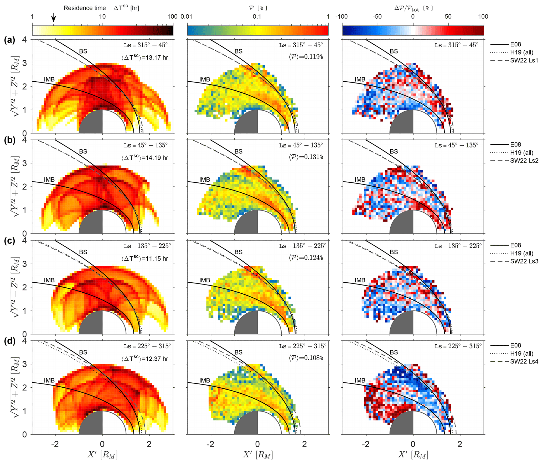
Figure 11Residence time (left) and probability 𝒫 of detecting MM-like structures (middle) at Mars, and departure from total detection probability (right), with respect to Mars season (binned by Ls). (a) Ls = [315–45∘] = Ls1. (b) Ls = [45–135∘] = Ls2. (c) Ls = [135–225∘] = Ls3. (d) Ls = [225–315∘] = Ls4. The percentage difference is calculated as , with positive hot-hued (negative cold-hued) values showing where 𝒫Ls>𝒫tot (𝒫Ls<𝒫tot). The total rate 𝒫tot is taken from Fig. 3b. Bow shock average positions are shown as dotted lines (Hall et al., 2019, all points, noted H19) and as dashed lines (Simon Wedlund et al., 2022a, for each Ls range, noted SW22). See also caption of Fig. 3 for other details.
3.2.4 Dependence on season (Ls)
Dependence of MM-like structures on Martian season is presented in Fig. 11, with residence times on the left, detection probabilities in the middle and percentage departures from the total detection probability on the right, as before. In contrast to MY discrimination, the average residence times in a grid cell is quite similar for all four Ls ranges considered, with 〈ΔTsc〉∼12 h per grid cell, with the smallest residence time for Ls3= [135–225∘] (see also Fig. 7f and Table 3). This is due to a combination of relatively large spatial extension for the orbit and missing that Ls range during MY32 (see Fig. 4). Conversely, the highest residence time is for Ls2= [45–135∘] because of an orbital coverage less spatially extended in space and despite the Ls range being also missed during MY32.
The detection probabilities 𝒫 (middle panels, ignoring cells for which ΔTsc<2 h) display a rather similar behaviour for all Ls ranges with two main distribution loci: one around the shock and the other immediately upstream of the IMB. The Ls range [Ls4=225–315∘] (Fig. 11d) includes perihelion condition (, local maximum of EUV flux) as well as the peak of exospheric H density (; see Halekas and McFadden, 2021). It seems to contain, overall, smaller detection probabilities in the locus closest to the IMB than at aphelion (, local minimum of EUV flux, included in Fig. 11b). This is in agreement with the findings of Sect. 3.2.3, where larger EUV flux levels create noticeably less MM-like structures in the subsolar magnetosheath than smaller EUV levels do, as a likely result of a combination of comparatively lower plasma-β (Rojas Mata et al., 2022) leading to PCWs being the fastest growing mode in those conditions (Ruhunusiri et al., 2018), and, possibly, non-gyrotropic effects.
From a statistical viewpoint, Fig. 11b for Ls2 (respectively, Fig. 11d for Ls4) resembles most Fig. 9a (Fig. 9b). This is in line with the conclusions of Sect. 3.2.1 and Fig. 7e, where we emphasised that the Ls2 (Ls4) range is representative of low (high) EUV flux conditions. Moreover, Ls1 and Ls3 ranges are mutually comparable as they have roughly similar PDFs over a rather large EUV flux range: these two ranges thus mostly display changes due to seasonal effects. In this view, the Ls1 range has a more evenly spread distribution of MM-like events around the shock, whereas the Ls3 range displays comparatively sharper and less spatially extended features. It is interesting to note that, in contrast to other Ls ranges, the Ls4 range displays its highest detection probability in the deep magnetospheric tail just behind the IMB (see Fig. 11d, middle plot and red region on the rightmost plot). This is a characteristic we have seen most often displayed at high EUV fluxes (Fig. 9b) and during MY33 (Fig. 8b), which is consistent with this Ls range encompassing perihelion conditions (see Fig. 4).
In this paper, we have aimed at creating maps of detection probabilities of mirror-mode (MM)-like structures in the Martian environment, in a quest to better characterise MMs across weakly magnetised and unmagnetised planets. Because magnetometers are a common instrument on space missions, with similar resolution and characteristics, they are an ideal tool to compare specific low-frequency wave modes such as the ubiquitous MMs. This study is the first of two at Mars and Venus (see Volwerk et al., 2022, for the companion paper as Part 2), using for the first time the same magnetic-field-only detection criteria and the same representation at both planets. At Mars, we use the MAVEN data between 2014 and 2021, and at Venus, we use the Venus Express data between 2006 and 2014.
We examined how these detection probability maps in MSO coordinates change with respect to MY, atmospheric seasons (Ls) and solar EUV flux. Overall, MM-like structures are mostly confined to two regions: one immediately behind the bow shock, especially at larger solar zenith angles (SZA), and one closer to the induced magnetospheric boundary (IMB). This picture is in good agreement with previous studies at Mars (Bertucci et al., 2004; Espley et al., 2004; Simon Wedlund et al., 2022b) and Venus (Volwerk et al., 2008, 2016; Fränz et al., 2017; Rojas Mata et al., 2022).
We linked the most dramatic changes in the spatial distribution of MM-like structures with solar EUV flux variations. First, the regions of high MM-like occurrences contract and expand following the EUV flux-led variations of the shock and the IMB. Second, with similar statistics, the higher the EUV flux (and, to a certain extent, solar activity), the lower the probability of detecting MM-like events around the shock and the dayside IMB. Simultaneously, high EUV flux conditions contain larger detection probabilities in the magnetospheric tail, downstream of the IMB.
The first behaviour contradicts the simple picture that, as the solar EUV flux and ionisation levels increase in the extended exosphere, the creation of additional pickup ions may lead to an increased ion temperature anisotropy in the entire volume of space, both in the solar wind and in the magnetosheath – a favourable condition for MM generation. We highlight two possible reasons that may explain the discrepancy: the potential predominance of low plasma-β at high solar activity (Rojas Mata et al., 2022), leading to an increased presence of PCWs at and around perihelion (Romanelli et al., 2016), favouring their growth over MMs, and, possibly, the non-gyrotropic nature of pickup ions at Mars and Venus (Coates, 2011). Investigating in full the reason(s) of this discrepancy could be achieved by the full use of the plasma suite on board MAVEN, with the Solar Wind Ion Analyzer (SWIA) and the Solar Wind Electron Analyzer (SWEA) complementing the magnetometer data.
The second behaviour above is also reflected in changes with respect to atmospheric seasons (or solar longitude Ls): we have found that the northern hemisphere winter season (encompassing perihelion conditions, and thus higher EUV fluxes) contained less MM-like structures around the shock with compressive signatures more often observed in the magnetospheric tail (nightside downstream of the IMB). Such structures in this unusual region pose questions as to their nature, origin and characteristics and will need a dedicated study to ascertain them, preferably with the full plasma suite.
We emphasise several possible tracks to continue and expand on this first work. First, this work should be redone with coincident plasma/magnetometer measurements. Although we may lose somewhat in temporal resolution with respect to magnetic field measurements (SWIA has a 4–8 s resolution in the magnetosheath, whereas SWEA can reach down to 2 s), we will gain the certitude of a B–N antiphase behaviour, which is a necessary characteristic of MMs (see Jin et al., 2022, for a recent study using SWIA). Complementary techniques such as using transport ratios to characterise the low-frequency wave environment (Song et al., 1994) could also usefully be applied to the full MAVEN dataset, as shown early in the mission (Ruhunusiri et al., 2015). Comparing all of these results with our present ones will give a measure of the accuracy of the B-field-only method over more foolproof methods and may help reinterpret past and present datasets from a new perspective. Second, to expand our current study, we should also look at the dependence of MM detection probabilities with respect to upstream solar wind conditions (density, velocity, magnitude and orientation of BIMF), as well as the shock nature (quasi-parallel or quasi-perpendicular). The latter would help in determining the respective effects of unstable pickup ion distributions and quasi-perpendicular shock heating in the generation of the temperature anisotropy at the origin of MM structures. All studies could finally be performed in Mars Solar Electric coordinates, oriented along the solar wind convection electric field.
The calibrated MAVEN/MAG datasets are available from the NASA Planetary Data System (PDS) at https://doi.org/10.17189/1414178 (Lawton and Connerney, 2023; Connerney et al., 2015). The FISM-P Mars Solar Spectral Irradiance model is available at the LASP Interactive Solar Irradiance Datacenter (LISIRD) of the Laboratory for Atmospheric and Space Physics (https://lasp.colorado.edu/lisird/data/fism_p_ssi_mars, last access: 19 May 2023, Chamberlin et al., 2008; Thiemann et al., 2017) and at https://doi.org/10.17189/1517691 (Version 2.21, MAVEN Release 28, released 9 February 2022, Connerney et al., 2015) through NASA PDS archives. Predicted bow shock times, spatial coordinates and shock geometry (θBn) for the 2014–2021 dataset (up to Mars Year 35) are available on Zenodo at https://doi.org/10.5281/zenodo.5725288 (Version 3, Simon Wedlund et al., 2021).
CSW and MV instigated the project, made the calculations and the main interpretation, drew the figures, and wrote the main text for this study. CM, SRM, GSW, YF, JH, DRC, CB and JE contributed to the data validation and interpretation, numerous ideas and science discussions, and helped with the writing of the main text and text revision.
The contact author has declared that none of the authors has any competing interests.
Publisher’s note: Copernicus Publications remains neutral with regard to jurisdictional claims in published maps and institutional affiliations.
Cyril Simon Wedlund and Martin Volwerk thank the Austrian Science Fund (FWF), and SRM thanks the Swedish National Space Agency for their support. The authors thank Charlotte Götz (Northumbria University, Newcastle, UK) and Arnaud Beth (Imperial College London, UK) for useful feedback on magnetosonic waves, as well as Christian Möstl, Zoltan Vörös, Luis Preisser, Owen Roberts and Adriana Settino (IWF-ÖAW, Graz) for useful discussions with respect to bow shock crossings, Earth's turbulence, mirror modes and magnetosheath jets. The authors thank Emmanuel Penou for help and access to the CLWeb viewing and analysis software (v16.09) from IRAP/Observatoire Midi-Pyrénées. This research was supported by the International Space Science Institute (ISSI) in Bern, through ISSI International Team project no. 517 (Towards a Unifying Model for Magnetic Depressions in Space Plasmas, led by MV) and project no. 499 (Similarities and Differences in the Plasma at Comets and Mars, led by Charlotte Götz).
This research has been supported by the Austrian Science Fund (project no. P32035-N36) and the Swedish National Space Agency (contract nos. 145/19 and 79/19).
This paper was edited by Dalia Buresova and reviewed by two anonymous referees.
Ala-Lahti, M. M., Kilpua, E. K. J., Dimmock, A. P., Osmane, A., Pulkkinen, T., and Souček, J.: Statistical analysis of mirror mode waves in sheath regions driven by interplanetary coronal mass ejection, Ann. Geophys., 36, 793–808, https://doi.org/10.5194/angeo-36-793-2018, 2018. a
Allison, M. and McEwen, M.: A post-Pathfinder evaluation of areocentric solar coordinates with improved timing recipes for Mars seasonal/diurnal climate studies, Planet. Space Sci., 48, 215–235, https://doi.org/10.1016/S0032-0633(99)00092-6, 2000. a, b
Bertucci, C., Mazelle, C., Crider, D. H., Mitchell, D. L., Sauer, K., Acuña, M. H., Connerney, J. E. P., Lin, R. P., Ness, N. F., and Winterhalter, D.: MGS MAG/ER observations at the magnetic pileup boundary of Mars: draping enhancement and low frequency waves, Adv. Space Res., 33, 1938–1944, https://doi.org/10.1016/j.asr.2003.04.054, 2004. a, b, c, d
Brinca, A. L. and Romeiras, F. J.: On the stability of stationary nongyrotropic distribution functions: Coupling and purely growing waves, J. Geophys. Res., 103, 9275–9284, https://doi.org/10.1029/97JA01995, 1998. a
Chamberlin, P. C., Woods, T. N., and Eparvier, F. G.: Flare Irradiance Spectral Model (FISM): Flare component algorithms and results, Space Weather, 6, 1–16, https://doi.org/10.1029/2007SW000372, 2008 . a
Coates, A.: Pickup Ion Observations at Solar System Bodies, in: Advances in Geosciences, Planet. Sci., 25, 11–28, https://doi.org/10.1142/9789814355377_0002, 2011. a, b
Coates, A. J., Johnstone, A. D., and Neubauer, F. M.: Cometary ion pressure anisotropies at comets Halley and Grigg-Skjellerup, J. Geophys. Res., 101, 27573–27584, https://doi.org/10.1029/96JA02524, 1996. a
Connerney, J. E. P., Espley, J., Lawton, P., Murphy, S., Odom, J., Oliversen, R., and Sheppard, D.: The MAVEN Magnetic Field Investigation, Space Sci. Rev., 195, 257–291, https://doi.org/10.1007/s11214-015-0169-4, 2015. a, b, c, d
Delva, M., Mazelle, C., and Bertucci, C.: Upstream Ion Cyclotron Waves at Venus and Mars, Space Sci. Rev., 162, 5–24, https://doi.org/10.1007/s11214-011-9828-2, 2011. a
Dimmock, A. P., Osmane, A., Pulkkinen, T. I., and Nykyri, K.: A statistical study of the dawn-dusk asymmetry of ion temperature anisotropy and mirror mode occurrence in the terrestrial dayside magnetosheath using THEMIS data, J. Geophys. Res.-Space, 120, 5489–5503, https://doi.org/10.1002/2015JA021192, 2015. a
Dong, C., Bougher, S. W., Ma, Y., Toth, G., Lee, Y., Nagy, A. F., Tenishev, V., Pawlowski, D. J., Combi, M. R., and Najib, D.: Solar wind interaction with the Martian upper atmosphere: Crustal field orientation, solar cycle, and seasonal variations, J. Geophys. Res.-Space, 120, 7857–7872, https://doi.org/10.1002/2015JA020990, 2015. a
Dubinin, E. and Fraenz, M.: Ultra-Low-Frequency Waves at Venus and Mars, Washington DC American Geophysical Union Geophysical Monograph Series, American Geophysical Union (AGU), ISBN: 9781119055006, 216, 343–364, https://doi.org/10.1002/9781119055006.ch20, 2016. a
Edberg, N. J. T., Lester, M., Cowley, S. W. H., and Eriksson, A. I.: Statistical analysis of the location of the Martian magnetic pileup boundary and bow shock and the influence of crustal magnetic fields: J. Geophys. Res., 113, A08206, https://doi.org/10.1029/2008JA013096, 2008. a, b, c, d, e, f, g, h
Edberg, N. J. T., Brain, D. A., Lester, M., Cowley, S. W. H., Modolo, R., Fränz, M., and Barabash, S.: Plasma boundary variability at Mars as observed by Mars Global Surveyor and Mars Express, Ann. Geophys., 27, 3537–3550, https://doi.org/10.5194/angeo-27-3537-2009, 2009. a, b
Erdős, G. and Balogh, A.: Statistical properties of mirror mode structures observed by Ulysses in the magnetosheath of Jupiter, J. Geophys. Res.-Space, 101, 1–12, https://doi.org/10.1029/95JA02207, 1996. a, b, c
Erkaev, N. V., Schaffenberger, W., Biernat, H. K., Farrugia, C. J., and Vogl, D. F.: Analysis of mirror modes convected from the bow shock to the magnetopause, Planet. Space Sci., 49, 1359–1364, https://doi.org/10.1016/S0032-0633(01)00057-5, 2001. a, b
Espley, J. R., Cloutier, P. A., Brain, D. A., Crider, D. H., and Acuña, M. H.: Observations of low-frequency magnetic oscillations in the Martian magnetosheath, magnetic pileup region, and tail, J. Geophys. Res.-Space, 109, A07213, https://doi.org/10.1029/2003JA010193, 2004. a
Forbes, J. M., Lemoine, F. G., Bruinsma, S. L., Smith, M. D., and Zhang, X.: Solar flux variability of Mars' exosphere densities and temperatures, Geophys. Res. Lett., 35, L01201, https://doi.org/10.1029/2007GL031904, 2008. a
Fowler, C. M., Hanley, K. G., McFadden, J. P., Chaston, C. C., Bonnell, J. W., Halekas, J. S., Espley, J. R., DiBraccio, G. A., Schwartz, S. J., Mazelle, C., Mitchell, D. L., Xu, S., and Lillis, R. J.: MAVEN Observations of Low Frequency Steepened Magnetosonic Waves and Associated Heating of the Martian Nightside Ionosphere, J. Geophys. Res.-Space, 126, e2021JA029615, https://doi.org/10.1029/2021JA029615, 2021. a
Fränz, M., Echer, E., Marques de Souza, A., Dubinin, E., and Zhang, T. L.: Ultra low frequency waves at Venus: Observations by the Venus Express spacecraft, Planet. Space Sci., 146, 55–65, https://doi.org/10.1016/j.pss.2017.08.011, 2017. a, b, c
Garnier, P., Jacquey, C., Gendre, X., Génot, V., Mazelle, C., Fang, X., Gruesbeck, J. R., Sánchez-Cano, B., and Halekas, J. S.: The Drivers of the Martian Bow Shock Location: A Statistical Analysis of Mars Atmosphere and Volatile EvolutioN and Mars Express Observations, J. Geophys. Res.-Space, 127, e30147, https://doi.org/10.1029/2021JA030147, 2022. a
Gary, S. P.: The mirror and ion cyclotron anisotropy instabilities, J. Geophys. Res., 97, 8519, https://doi.org/10.1029/92JA00299, 1992. a
Gary, S. P.: Theory of Space Plasma Microinstabilities, Cambridge University Press, google-Books-ID: hMiulET5wpwC, Cambridge, Cambridge University Press, https://doi.org/10.1017/CBO9780511551512, 1993. a, b
Gary, S. P. and Winske, D.: Correlation function ratios and the identification of space plasma instabilities, J. Geophys. Res.-Space, 97, 3103–3111, https://doi.org/10.1029/91JA02752, 1992. a, b
Génot, V., Schwartz, S. J., Mazelle, C., Balikhin, M., Dunlop, M., and Bauer, T. M.: Kinetic study of the mirror mode, J. Geophys. Res., 106, 21611–21622, https://doi.org/10.1029/2000JA000457, 2001. a, b, c, d
Génot, V., Budnik, E., Jacquey, C., Dandouras, I., and Lucek, E.: Mirror modes observed with Cluster in the Earth's magnetosheath: statistical study and IMF/solar wind dependence, in: Advances in Geosciences, Vol. 14, 263–283, World Scientific Publishing Company, https://doi.org/10.1142/9789812836205_0019, 2009. a, b, c
Glassmeier, K. H., Motschmann, U., Mazelle, C., Neubauer, F. M., Sauer, K., Fuselier, S. A., and Acuña, M. H.: Mirror modes and fast magnetoacoustic waves near the magnetic pileup boundary of comet P/Halley, J. Geophys. Res.-Space, 98, 20955–20964, https://doi.org/10.1029/93JA02582, 1993. a, b
Gruesbeck, J. R., Espley, J. R., Connerney, J. E. P., DiBraccio, G. A., Soobiah, Y. I., Brain, D., Mazelle, C., Dann, J., Halekas, J., and Mitchell, D. L.: The Three-Dimensional Bow Shock of Mars as Observed by MAVEN, J. Geophys. Res.-Space, 123, 4542–4555, https://doi.org/10.1029/2018JA025366, 2018. a, b, c, d, e
Halekas, J. S.: Seasonal variability of the hydrogen exosphere of Mars, J. Geophys. Res.-Planet., 122, 901–911, https://doi.org/10.1002/2017JE005306, 2017. a
Halekas, J. S. and McFadden, J. P.: Using Solar Wind Helium to Probe the Structure and Seasonal Variability of the Martian Hydrogen Corona, J. Geophys. Res.-Planet., 126, e07049, https://doi.org/10.1029/2021JE007049, 2021. a, b
Halekas, J. S., Taylor, E. R., Dalton, G., Johnson, G., Curtis, D. W., McFadden, J. P., Mitchell, D. L., Lin, R. P., and Jakosky, B. M.: The Solar Wind Ion Analyzer for MAVEN, Space Sci. Rev., 195, 125–151, https://doi.org/10.1007/s11214-013-0029-z, 2015. a, b
Halekas, J. S., Brain, D. A., Luhmann, J. G., DiBraccio, G. A., Ruhunusiri, S., Harada, Y., Fowler, C. M., Mitchell, D. L., Connerney, J. E. P., Espley, J. R., Mazelle, C., and Jakosky, B. M.: Flows, Fields, and Forces in the Mars-Solar Wind Interaction, J. Geophys. Res.-Space, 122, 11320–11341, https://doi.org/10.1002/2017JA024772, 2017a. a, b
Halekas, J. S., Ruhunusiri, S., Harada, Y., Collinson, G., Mitchell, D. L., Mazelle, C., McFadden, J. P., Connerney, J. E. P., Espley, J. R., Eparvier, F., Luhmann, J. G., and Jakosky, B. M.: Structure, dynamics, and seasonal variability of the Mars-solar wind interaction: MAVEN Solar Wind Ion Analyzer in-flight performance and science results, J. Geophys. Res.-Space, 122, 547–578, https://doi.org/10.1002/2016JA023167, 2017b. a, b, c, d, e
Halekas, J. S., Ruhunusiri, S., Vaisberg, O. L., Harada, Y., Espley, J., Mitchell, D. L., Mazelle, C., Romanelli, N., DiBraccio, G. A., and Brain, D. A.: Properties of Plasma Waves Observed Upstream from Mars, World Library Catalog, Earth and Space Science Open Archive Section, Sol. Syst. Phys., 125, e2020JA028221, https://doi.org/10.1029/2020JA028221, 2020. a
Hall, B. E. S., Lester, M., Sánchez-Cano, B., Nichols, J. D., Andrews, D. J., Edberg, N. J. T., Opgenoorth, H. J., Fränz, M., Holmström, M., Ramstad, R., Witasse, O., Cartacci, M., Cicchetti, A., Noschese, R., and Orosei, R.: Annual variations in the Martian bow shock location as observed by the Mars Express mission, J. Geophys. Res.-Space, 121, 11474–11494, https://doi.org/10.1002/2016JA023316, 2016. a, b
Hall, B. E. S., Sánchez-Cano, B., Wild, J. A., Lester, M., and Holmström, M.: The Martian Bow Shock Over Solar Cycle 23–24 as Observed by the Mars Express Mission, J. Geophys. Res.-Space, 124, 4761–4772, https://doi.org/10.1029/2018JA026404, 2019. a, b, c, d, e, f, g, h, i
Hasegawa, A.: Drift Mirror Instability in the Magnetosphere, Phys. Fluids, 12, 2642, https://doi.org/10.1063/1.1692407, 1969. a, b
Hoilijoki, S., Palmroth, M., Walsh, B. M., Pfau-Kempf, Y., von Alfthan, S., Ganse, U., Hannuksela, O., and Vainio, R.: Mirror modes in the Earth's magnetosheath: Results from a global hybrid-Vlasov simulation, J. Geophys. Res.-Space, 121, 4191–4204, https://doi.org/10.1002/2015JA022026, 2016. a
Jarvinen, R., Kallio, E., and Pulkkinen, T. I.: Ultra-low Frequency Foreshock Waves and Ion Dynamics at Mars, J. Geophys. Res.-Space, 127, e30078, https://doi.org/10.1029/2021JA030078, 2022. a
Jin, T., Lei, L., Yiteng, Z., Lianghai, X., and Fuhao, Q.: Statistical Analysis of the Distribution and Evolution of Mirror Structures in the Martian Magnetosheath, Astrophys. J., 929, 1–14, https://doi.org/10.3847/1538-4357/ac5f00, 2022. a, b, c, d
Joy, S. P., Kivelson, M. G., Walker, R. J., Khurana, K. K., Russell, C. T., and Paterson, W. R.: Mirror mode structures in the Jovian magnetosheath, J. Geophys. Res., 111, A12212, https://doi.org/10.1029/2006JA011985, 2006. a, b
Karlsson, T., Heyner, D., Volwerk, M., Morooka, M., Plaschke, F., Goetz, C., and Hadid, L.: Magnetic Holes in the Solar Wind and Magnetosheath Near Mercury, J. Geophys. Res.-Space, 126, e28961, https://doi.org/10.1029/2020JA028961, 2021. a
Lucek, E. A., Dunlop, M. W., Balogh, A., Cargill, P., Baumjohann, W., Georgescu, E., Haerendel, G., and Fornacon, K.-H.: Identification of magnetosheath mirror modes in Equator-S magnetic field data, Ann. Geophys., 17, 1560–1573, https://doi.org/10.1007/s00585-999-1560-9, 1999. a, b, c
Madanian, H., Halekas, J. S., Mazelle, C. X., Omidi, N., Espley, J. R., Mitchell, D. L., and McFadden, J. P.: Magnetic Holes Upstream of the Martian Bow Shock: MAVEN Observations, J. Geophys. Res.-Space, 125, e2019JA027198, https://doi.org/10.1029/2019JA027198, 2020. a, b
Mazelle, C., Rème, H., Sauvaud, J. A., d'Uston, C., Carlson, C. W., Anderson, K. A., Curtis, D. W., Lin, R. P., Korth, A., Mendis, D. A., Neubauer, F. M., Glassmeier, K. H., and Raeder, J.: Analysis of suprathermal electron properties at the magnetic pile-up boundary of comet P/Halley, Geophys. Res. Lett., 16, 1035–1038, https://doi.org/10.1029/GL016i009p01035, 1989. a
Mazelle, C., Belmont, G., Glassmeier, K. H., Le Quéau, D., and Rème, H.: Ultra low frequency waves at the magnetic pile-up boundary of comet P/Halley, Adv. Space Res., 11, 73–77, https://doi.org/10.1016/0273-1177(91)90014-B, 1991. a, b
Mazelle, C., Winterhalter, D., Sauer, K., Trotignon, J., Acuña, M., Baumgärtel, K., Bertucci, C., Brain, D., Brecht, S., Delva, M., Dubinin, E., Øieroset, M., and Slavin, J.: Bow Shock and Upstream Phenomena at Mars, Space Sci. Revi., 111, 115–181, https://doi.org/10.1023/B:SPAC.0000032717.98679.d0, 2004. a, b, c, d
Mitchell, D. L., Mazelle, C., Sauvaud, J.-A., Thocaven, J.-J., Rouzaud, J., Fedorov, A., Rouger, P., Toublanc, D., Taylor, E., Gordon, D., Robinson, M., Heavner, S., Turin, P., Diaz-Aguado, M., Curtis, D. W., Lin, R. P., and Jakosky, B. M.: The MAVEN Solar Wind Electron Analyzer, Space Sci. Rev., 200, 495–528, https://doi.org/10.1007/s11214-015-0232-1, 2016. a
Motschmann, U., Kafemann, H., and Scholer, M.: Nongyrotropy in magnetoplasmas: simulation of wave excitation and phase-space diffusion, Ann. Geophys., 15, 603–613, https://doi.org/10.1007/s00585-997-0603-3, 1997. a
Lawton, P. and Connerney, J.: MAVEN MAG Calibrated Data Bundle, NASA [data set], https://doi.org/10.17189/1414178, 2023. a
Price, C. P.: Mirror waves driven by newborn ion distributions, J. Geophys. Res., 94, 15001–15009, https://doi.org/10.1029/JA094iA11p15001, 1989. a, b
Price, C. P., Swift, D. W., and Lee, L.-C.: Numerical simulation of nonoscillatory mirror waves at the Earth's magnetosheath, J. Geophys. Res.-Space, 91, 101–112, https://doi.org/10.1029/JA091iA01p00101, 1986. a
Rojas Mata, S., Stenberg Wieser, G., Futaana, Y., Bader, A., Persson, M., Fedorov, A., and Zhang, T.: Proton Temperature Anisotropies in the Venus Plasma Environment During Solar Minimum and Maximum, J. Geophys. Res.-Space, 127, e29611, https://doi.org/10.1029/2021JA029611, 2022. a, b, c, d, e, f, g
Romanelli, N., Bertucci, C., Gómez, D., Mazelle, C., and Delva, M.: Proton cyclotron waves upstream from Mars: Observations from Mars Global Surveyor, Planet. Space Sci., 76, 1–9, https://doi.org/10.1016/j.pss.2012.10.011, 2013. a
Romanelli, N., Mazelle, C., Chaufray, J. Y., Meziane, K., Shan, L., Ruhunusiri, S., Connerney, J. E. P., Espley, J. R., Eparvier, F., Thiemann, E., Halekas, J. S., Mitchell, D. L., McFadden, J. P., Brain, D., and Jakosky, B. M.: Proton cyclotron waves occurrence rate upstream from Mars observed by MAVEN: Associated variability of the Martian upper atmosphere, J. Geophys. Res.-Space, 121, 11113–11128, https://doi.org/10.1002/2016JA023270, 2016. a, b, c, d, e
Romeo, O. M., Romanelli, N., Espley, J. R., Mazelle, C., DiBraccio, G. A., Gruesbeck, J. R., and Halekas, J. S.: Variability of Upstream Proton Cyclotron Wave Properties and Occurrence at Mars Observed by MAVEN, J. Geophys. Res.-Space, 126, e28616, https://doi.org/10.1029/2020JA028616, 2021. a, b
Ruhunusiri, S., Halekas, J. S., Connerney, J. E. P., Espley, J. R., McFadden, J. P., Larson, D. E., Mitchell, D. L., Mazelle, C., and Jakosky, B. M.: Low-frequency waves in the Martian magnetosphere and their response to upstream solar wind driving conditions, Geophys. Res. Lett., 42, 8917–8924, https://doi.org/10.1002/2015GL064968, 2015. a, b, c, d, e, f
Ruhunusiri, S., Halekas, J. S., Espley, J. R., Eparvier, F., Brain, D., Mazelle, C., Harada, Y., DiBraccio, G. A., Thiemann, E. M. B., Larson, D. E., Mitchell, D. L., Jakosky, B. M., and Sulaiman, A. H.: One-Hertz Waves at Mars: MAVEN Observations, J. Geophys. Res.-Space, 123, 3460–3476, https://doi.org/10.1029/2017JA024618, 2018. a
Schwartz, S. J., Burgess, D., and Moses, J. J.: Low-frequency waves in the Earth's magnetosheath: present status, Ann. Geophys., 14, 1134–1150, https://doi.org/10.1007/s00585-996-1134-z, 1997. a
Shan, L., Tsurutani, B. T., Ohsawa, Y., Mazelle, C., Huang, C., Du, A., Ge, Y. S., and Lu, Q.: Observational Evidence for Fast Mode Periodic Small-scale Shocks: A New Type of Plasma Phenomenon, Astrophys. J. Lett., 905, 1–6, https://doi.org/10.3847/2041-8213/abcb02, 2020. a, b
Simon Wedlund, C., Volwerk, M., Beth, A., Mazelle, C., Möstl, C., Halekas, J., Gruesbeck, J., and Rojas-Castillo, D.: Predicted times, spatial coordinates of bow shock crossings and shock geometry at Mars from the NASA/MAVEN mission, using spacecraft ephemerides and magnetic field data, with a predictor-corrector algorithm (Version 3), Zenodo [data set] https://doi.org/10.5281/zenodo.6320518, 2021. a, b
Simon Wedlund, C., Volwerk, M., Beth, A., Mazelle, C., Möstl, C., Halekas, J., Gruesbeck, J. R., and Rojas-Castillo, D.: A Fast Bow Shock Location Predictor-Estimator From 2D and 3D Analytical Models: Application to Mars and the MAVEN Mission, J. Geophys. Res.-Space, 127, e2021JA029942, https://doi.org/10.1029/2021JA029942, 2022a. a, b, c, d, e, f, g, h, i, j, k, l, m, n, o, p, q, r, s
Simon Wedlund, C., Volwerk, M., Mazelle, C., Halekas, J., Rojas-Castillo, D., Espley, J., and Möstl, C.: Making Waves: Mirror Mode Structures Around Mars Observed by the MAVEN Spacecraft, J. Geophys. Res.-Space, 127, e2021JA029811, https://doi.org/10.1029/2021JA029811, 2022b. a, b, c, d, e, f, g, h, i, j, k, l, m, n, o, p, q, r, s, t, u, v, w
Song, P., Russell, C. T., and Gary, S. P.: Identification of low-frequency fluctuations in the terrestrial magnetosheath, J. Geophys. Res., 99, 6011, https://doi.org/10.1029/93JA03300, 1994. a, b, c
Sonnerup, B. U. Ö. and Scheible, M.: Minimum and Maximum Variance Analysis, in: Analysis Methods for Multi-Spacecraft Data, no. SR-001 in ISSI Scientific Report, ISSI/ESA, ESA Publications Division, the Netherlands, 185–220, ISBN: 1608-280X, 1998. a
Soucek, J., Lucek, E., and Dandouras, I.: Properties of magnetosheath mirror modes observed by Cluster and their response to changes in plasma parameters, J. Geophys. Res.-Space, 113, A04203, https://doi.org/10.1029/2007JA012649, 2008. a, b, c
Szegö, K., Glassmeier, K.-H., Bingham, R., Bogdanov, A., Fischer, C., Haerendel, G., Brinca, A., Cravens, T., Dubinin, E., Sauer, K., Fisk, L., Gombosi, T., Schwadron, N., Isenberg, P., Lee, M., Mazelle, C., Möbius, E., Motschmann, U., Shapiro, V. D., Tsurutani, B., and Zank, G.: Physics of Mass Loaded Plasmas, Space Sci. Rev., 94, 429–671, https://doi.org/10.1023/A:1026568530975, 2000. a
Thiemann, E. M. B., Chamberlin, P. C., Eparvier, F. G., Templeman, B., Woods, T. N., Bougher, S. W., and Jakosky, B. M.: The MAVEN EUVM model of solar spectral irradiance variability at Mars: Algorithms and results, J. Geophys. Res.-Space, 122, 2748–2767, https://doi.org/10.1002/2016JA023512, 2017. a, b, c
Trainer, M. G., Wong, M. H., McConnochie, T. H., Franz, H. B., Atreya, S. K., Conrad, P. G., Lefèvre, F., Mahaffy, P. R., Malespin, C. A., Manning, H. L. K., Martín-Torres, J., Martínez, G. M., McKay, C. P., Navarro-González, R., Vicente-Retortillo, Á., Webster, C. R., and Zorzano, M.-P.: Seasonal Variations in Atmospheric Composition as Measured in Gale Crater, Mars, J. Geophys. Res.-Planet., 124, 3000–3024, https://doi.org/10.1029/2019JE006175, 2019. a
Treumann, R. A., Jaroschek, C. H., Constantinescu, O. D., Nakamura, R., Pokhotelov, O. A., and Georgescu, E.: The strange physics of low frequency mirror mode turbulence in the high temperature plasma of the magnetosheath, Nonlin. Processes Geophys., 11, 647–657, https://doi.org/10.5194/npg-11-647-2004, 2004. a, b
Trotignon, J., Mazelle, C., Bertucci, C., and Acuña, M.: Martian shock and magnetic pile-up boundary positions and shapes determined from the Phobos 2 and Mars Global Surveyor data sets, Planet. Space Sci., 54, 357–369, https://doi.org/10.1016/j.pss.2006.01.003, 2006. a, b
Tsurutani, B. T.: Comets: a Laboratory for Plasma Waves and Instabilities, in: Cometary Plasma Processes, 189–209, American Geophysical Union (AGU), https://doi.org/10.1029/GM061p0189, 1991. a
Tsurutani, B. T., Thorne, R. M., Smith, E. J., Gosling, J. T., and Matsumoto, H.: Steepened magnetosonic waves at comet Giacobini-Zinner, J. Geophys. Res.-Space, 92, 11074–11082, https://doi.org/10.1029/JA092iA10p11074, 1987. a, b
Tsurutani, B. T., Lakhina, G. S., Smith, E. J., Buti, B., Moses, S. L., Coroniti, F. V., Brinca, A. L., Slavin, J. A., and Zwickl, R. D.: Mirror mode structures and ELF plasma waves in the Giacobini-Zinner magnetosheath, Nonlin. Processes Geophys., 6, 229–234, https://doi.org/10.5194/npg-6-229-1999, 1999. a
Tsurutani, B. T., Lakhina, G. S., Verkhoglyadova, O. P., Echer, E., Guarnieri, F. L., Narita, Y., and Constantinescu, D. O.: Magnetosheath and heliosheath mirror mode structures, interplanetary magnetic decreases, and linear magnetic decreases: Differences and distinguishing features,: J. Geophys. Res., 116, A2, https://doi.org/10.1029/2010JA015913, 2011. a, b
Turner, J. M., Burlaga, L. F., Ness, N. F., and Lemaire, J. F.: Magnetic holes in the solar wind, J. Geophys. Res., 82, 1921, https://doi.org/10.1029/JA082i013p01921, 1977. a
Volwerk, M., Zhang, T. L., Delva, M., Vörös, Z., Baumjohann, W., and Glassmeier, K.-H.: Mirror-mode-like structures in Venus' induced magnetosphere, J. Geophys. Res., 113, E00B16, https://doi.org/10.1029/2008JE003154, 2008. a, b, c, d
Volwerk, M., Schmid, D., Tsurutani, B. T., Delva, M., Plaschke, F., Narita, Y., Zhang, T., and Glassmeier, K.-H.: Mirror mode waves in Venus's magnetosheath: solar minimum vs. solar maximum, Ann. Geophys., 34, 1099–1108, https://doi.org/10.5194/angeo-34-1099-2016, 2016. a, b, c, d, e, f, g, h, i, j, k
Volwerk, M., Mautner, D., Wedlund, C. S., Goetz, C., Plaschke, F., Karlsson, T., Schmid, D., Rojas-Castillo, D., Roberts, O. W., and Varsani, A.: Statistical study of linear magnetic hole structures near Earth, Ann. Geophys., 39, 239–253, https://doi.org/10.5194/angeo-39-239-2021, 2021. a
Volwerk, M., Simon Wedlund, C., Mautner, D., Rojas Mata, S., Stenberg Wieser, G., Futaana, Y., Mazelle, C., Rojas-Castillo, D., Bertucci, C., and Delva, M.: Statistical distribution of mirror mode-like structures in the magnetosheaths of unmagnetised planets: 2. Venus as observed by the Venus Express spacecraft, EGUsphere [preprint], https://doi.org/10.5194/egusphere-2022-645, 2022. a, b, c
Wilson III, L. B., Stevens, M. L., Kasper, J. C., Klein, K. G., Maruca, B. A., Bale, S. D., Bowen, T. A., Pulupa, M. P., and Salem, C. S.: The Statistical Properties of Solar Wind Temperature Parameters Near 1 au, Astrophys. J. Suppl. Ser., 236, 1–15, https://doi.org/10.3847/1538-4365/aab71c, 2018. a
Yamauchi, M., Hara, T., Lundin, R., Dubinin, E., Fedorov, A., Sauvaud, J. A., Frahm, R. A., Ramstad, R., Futaana, Y., Holmstrom, M., and Barabash, S.: Seasonal variation of Martian pick-up ions: Evidence of breathing exosphere, Planet. Space Sci., 119, 54–61, https://doi.org/10.1016/j.pss.2015.09.013, 2015. a, b