A comparison of Jason-2 plasmasphere electron content measurements with ground-based measurements

Previous studies utilizing the Global Positioning System (GPS) receivers aboard Jason satellites have performed measurements of plasmasphere electron content (PEC) by determining the total electron content (TEC) above these satellites, which are at altitudes of about 1340 km. This study uses similar methods to determine PEC for the Jason-2 receiver for 24 July 2011. These PEC values are compared to previous determinations of PEC from a chain of ground-based GPS receivers in Africa using the SCORPION method, with a nominal ionosphere–plasmasphere boundary at 1000 km. The Jason-2 PECs with elevations greater than 60^∘ were converted to equivalent vertical PEC and compared to SCORPION vertical PEC determinations. In addition, slant (off-vertical) PECs from Jason-2 were compared to a small set of nearly co-aligned ground-based slant PECs. The latter comparison avoids any conversion of Jason-2 slant PEC to equivalent vertical PEC, and it can be considered a more representative comparison. The mean difference between the vertical PEC (ground-based minus Jason-2 measurements) values is 0.82 ± 0.28 TEC units (1 TEC unit=10¹⁶ electrons m⁻²). Similarly, the mean difference between slant PEC values is 0.168 ± 0.924 TEC units. The Jason-2 slant PEC comparison method may provide a reliable determination for the plasmasphere baseline value for the ground-based receivers, especially if the ground stations are confined to only midlatitude or low-latitude regions, which can be affected by a non-negligible PEC baseline.

1 Introduction

The plasmasphere is a toroidal domain of cold plasma confined by the Earth's magnetic field and replenished by the ionosphere (e.g., Lunt et al., 1999a; Dent et al., 2006). Several instruments and methods have been utilized to determine the electron or ion content of the plasmasphere. Among these are the IMAGE (Imager for Magnetopause-to-Aurora Global Exploration) satellite's Radio Plasma Imager (Galkin et al., 2004) and Extreme Ultraviolet Imager (Sibanda et al., 2012), ground-based magnetometers (Dent et al., 2006), satellite-borne Global Positioning System (GPS) receivers for Jason-1 (Yizengaw et al., 2008; Lee et al., 2013) and CHAMP (CHAllenging Minisatellite Payload) (Gerzen et al., 2015), satellite-based tomography (Spencer and Mitchell, 2011), and ground-based GPS receivers using data assimilation (Scherliess et al., 2004) or methods for partitioning total electron content (TEC) into ionosphere and plasmasphere contributions (Mazzella et al., 2002, 2007; Anghel et al., 2009; Carrano et al., 2009).

More recently, Mazzella et al. (2017) have presented an evaluation of TEC partitioned into the ionosphere and plasmasphere contributions for a chain of GPS receivers in Africa, for 24 July 2011. Peak equivalent vertical ionosphere electron content (VIEC) ranged from about 14 TEC units (1 TEC unit=10¹⁶ electrons m⁻²) at the southernmost (most poleward) station to about 32 TEC units for near-equatorial stations, while derived peak vertical plasmasphere electron content (VPEC) ranged from about 1 to about 6 TEC units for these stations.

The ground-based TEC study for Africa was conducted using an extension of the Self-Calibration Of Range Error (SCORE) method (Bishop et al., 1994). SCORE employed consistency conditions for equivalent vertical TEC (VTEC) measurements at associated ionosphere penetration points (IPPs) for different lines of sight to determine the combined GPS satellite and ground-based GPS receiver biases. However, as noted by Lunt et al. (1999b) and Fremouw et al. (1998), the occurrence of significant plasmasphere electron content (PEC) affects this calibration process, producing systematic bias errors, with a latitudinal dependence for the sign and magnitude of the errors. Consequently, the SCORE method was generalized by the inclusion of a parametric representation of the plasmasphere, becoming SCORE for Plasmasphere and IONosphere (SCORPION) (Mazzella et al., 2002, 2007). The consistency conditions at associated IPPs were retained by SCORPION but applied using only the VIEC values derived from the slant (off-vertical) TEC after removal of the parameterized slant PEC for the corresponding lines of sight. The parameters for the plasmasphere representation are determined within the same process as the GPS biases.

Regarding the Africa study, utilization of a chain of receivers with overlapping coverage not only provides extensive latitudinal coverage but also enables an evaluation of consistency for diurnal VIEC and VPEC profiles between locations and determination of the “plasmasphere baseline”. The plasmasphere baseline is the local (at each station) spatially and temporally constant component of the observed slant plasmasphere electron content (SPEC). Its value is somewhat affected by limitations for the observational circumstances (the sky regions above the elevation threshold and the typical 1 d data coverage). This component can masquerade as a contribution to the receiver bias (Mazzella et al., 2007).

The ambiguity between the contributions of the plasmasphere baseline and the receiver bias to the raw measured GPS TEC arises from the formulation for the corrections to the GPS TEC measurements to obtain the VIEC:

$$\begin{array}{}\text{(1)}& \text{VIEC}={\displaystyle \frac{\text{STEC}-\text{SPEC}-\text{Bias}}{\text{SlFac}}},\end{array}$$

where STEC represents raw GPS slant TEC measurement, SPEC represents slant plasmasphere electron content, Bias represents combined receiver and GPS satellite bias, and SlFac (slant factor) represents the ratio of slant ionosphere electron content (SIEC) to VIEC.

The slant factor is typically a function solely of the elevation angle (ε) of the GPS satellite at the receiver station, using a representative “thin-shell” altitude (H_s) for the ionosphere (e.g., Lanyi and Roth, 1988, in an alternative equivalent mathematical form):

$$\begin{array}{}\text{(2)}& \text{SlFac}=\sec \left(\arcsin \left({\displaystyle \frac{R_{\mathrm{e}}\cdot \cos \left(\mathit{\epsilon }\right)}{R_{\mathrm{e}}+H_{\mathrm{s}}}}\right)\right),\end{array}$$

where R_e represents the Earth's radius. In the SCORPION method, SPEC is represented by a parametric model, with the values of the parameters being determined together with the biases from consistency conditions for the entire set of VIEC values (Mazzella et al., 2002). Because the plasmasphere contribution appears only in combination with the biases, a latitudinal chain or some other external condition must be utilized to appropriately apportion the (local) spatially and temporally constant component between the plasmasphere and the bias. (Note that this is true even if the plasmasphere representation has a unique relationship between the spatially/temporally varying plasmasphere amplitude and the baseline contribution, because the actual plasmasphere is not governed by such a relationship. This latter ambiguity has been denoted as the “evil twin” problem.)

This subsequent analysis, similar to that performed by Yizengaw et al. (2008) and Lee et al. (2013), has been conducted using Jason-2 GPS receiver data, specifically for Africa on the same day (24 July 2011, denoted “day 205, 2011”) as the previous ground-based case study (Mazzella et al., 2017) to evaluate PEC values for comparison with those SCORPION results. However, the Jason-2 orbital altitude is approximately 1340 km, and its PEC measurements only correspond to altitudes above this orbital altitude, while the SCORPION measurements incorporate a nominal ionosphere–plasmasphere boundary at 1000 km altitude (Mazzella, 2009). Thus, the SCORPION PEC measurements should be greater than the Jason-2 PEC measurements, but the magnitude of this difference can vary with the time allowed for replenishment of the plasmasphere, the level of solar flux, and even the directions of the lines of sight through the plasmasphere (associated with the magnetic field-line crossings and the varying distance to the plasmapause). (See, for example, Fig. 5 by Mazzella, 2009.)

2 Data analysis

2.1 Preliminary processing

The Jason-2 GPS receiver data were obtained from the Jet Propulsion Laboratory (JPL) (Komjathy and Haines, private communication, 2013) in Receiver INdependent EXchange (RINEX) format and were processed using components of the GPS Toolkit (GPSTk) developed by the Applied Research Laboratories (ARL) of The University of Texas at Austin (Tolman et al., 2004). The resulting TEC values (in TEC units) were further adjusted for relative GPS satellite biases, using the August 2011 values from the Center for Orbit Determination in Europe (CODE) of the Astronomical Institute of the University of Bern (Schaer and Feltens, 1998). (As noted by Mazzella et al., 2017, the August 2011 bias value for PRN 1 appeared to be more accurate than the July 2011 value, which was derived soon after the satellite launch.) These GPS TEC tabulations, separated into contiguous time segments for each GPS satellite, were reviewed and edited for any observed anomalies.

A separate component of the GPSTk was utilized to process the same RINEX file for the Jason-2 satellite locations, in three dimensions. The derived latitudes and longitudes were subsequently compared to those in the Geophysical Data Record (Dumont et al., 2011), with good agreement, and the derived radial coordinates were within 4 km of the semi-major axis value (7714.43 km) reported in the OSTM/Jason-2 Products Handbook (Dumont et al., 2011). The Jason-2 latitude and longitude values were matched to the corresponding GPS TEC samples, and augmented TEC tabulations were generated.

2.2 TEC calibration

For each of the contiguous GPS TEC data segments, the dispersive carrier phase (SP) was aligned to the dispersive group delay (SR), using unweighted averaging, to take advantage of the lower noise and multipath associated with the SP values. Because the intrinsic multipath profile for Jason-2 was quite good (Fig. 1), the multipath consistency correction (Andreasen et al., 2002) used for the ground-based receivers in Africa (Mazzella et al., 2017) was not applied. (This correction process also would have required information about the Jason-2 satellite attitude, to convert the GPS lines of sight into a satellite-referenced coordinate system, and further allowance for the effects of the Jason-2 solar panels, as potentially varying multipath contributors.)

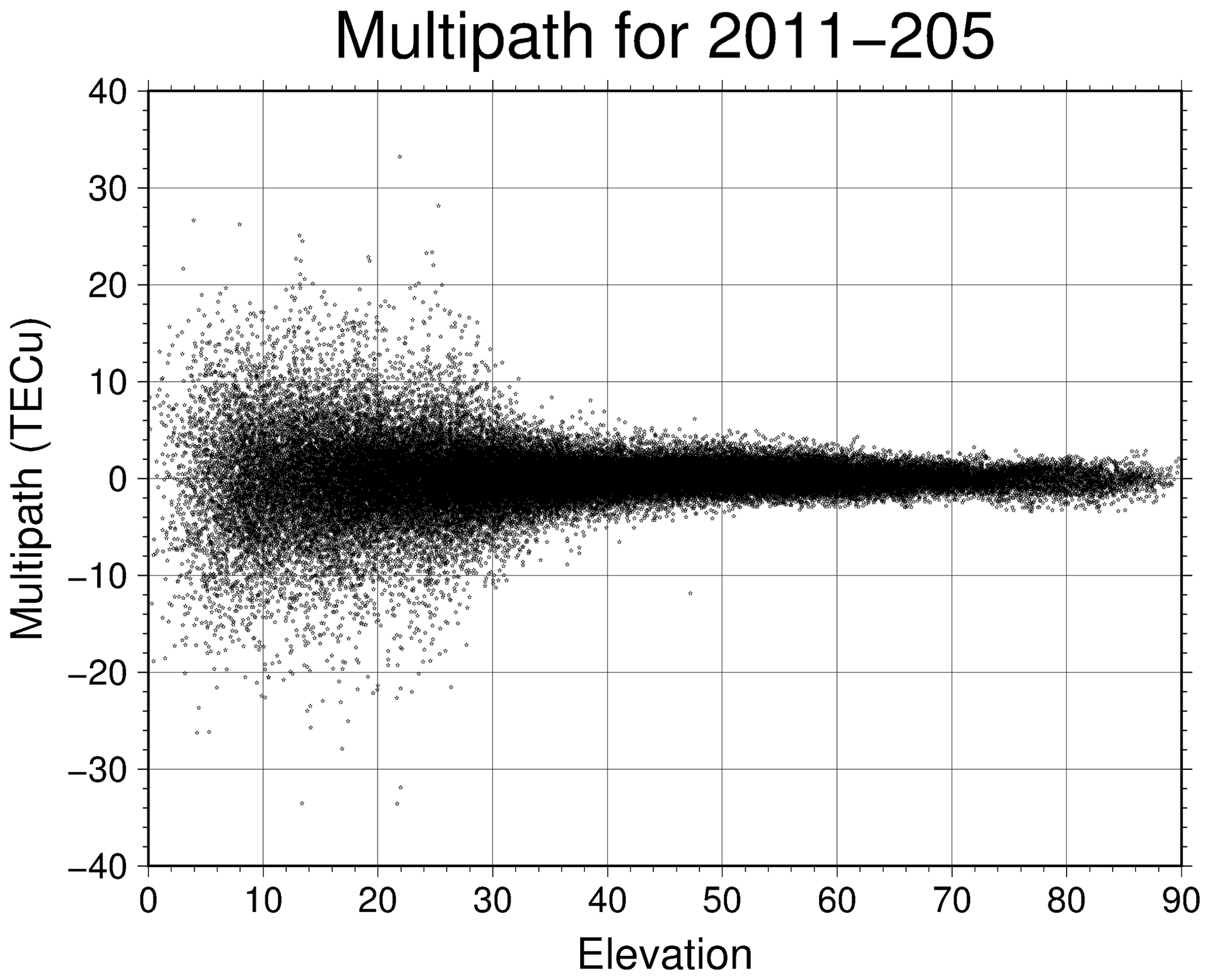
Figure 1 Multipath profile, in TEC units (“TECu”), for the Jason-2 satellite, derived from its GPS receiver data for day 205, 2011, using the differences between the SR and aligned SP.

The remaining determination of the Jason-2 receiver bias invoked the assumption that the minimum true SPEC is near zero, a method similar to that described by Yizengaw et al. (2008) and Lee et al. (2013), but with the additional consideration of the residual high-altitude, high-latitude electron content, using a model (Pedatella and Larson, 2010). The polar regions were specifically chosen for the receiver bias determination, because these were the regions with the intrinsically smallest SPEC values and thus any model corrections would also be small, so model errors would have less influence.

Figure 2 displays a north–south cross-section for Jason-2 (latitude 66^∘) and two GPS satellites (latitude 55^∘) at their (north) polar extremes to demonstrate both the lines of sight through the polar region and the associated elevation angles at the receiver. The innermost circle is the surface of the Earth, and the radial coordinate is gridded in Earth radius increments. Based on the geometry shown in Fig. 2, two subsets of the Jason-2 receiver data were selected, with one for each polar region. The selection criteria were as follows:

• absolute value of Jason-2 latitude ≥60^∘;

• poleward azimuths for lines of sight within ±90^∘ of the pole direction;

• elevations above 0^∘ for lines of sight to the GPS satellites;

• absolute value of GPS satellite latitudes $\ge \mathrm{45}{}^{\circ }$.

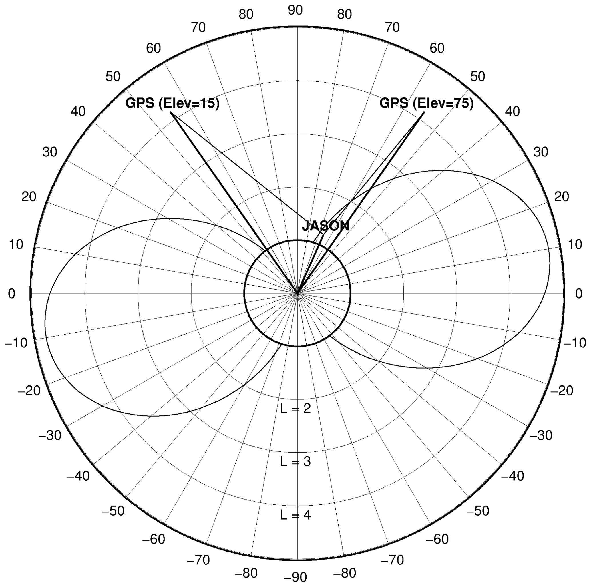
Figure 2 Viewing geometry for minimal expected SPEC occurrences for the Jason-2 GPS receiver, with a representative plasmapause indicated for L=4.8. The low-elevation, cross-polar line of sight can mainly avoid the plasmasphere, while the high-elevation line of sight can encounter the fringe of the plasmasphere, depending on the relative orientation of the geographic and geomagnetic poles.

The poleward azimuth criterion is intended to eliminate cases like the “Elev=75” case displayed in Fig. 2, which would have the possibility of grazing the plasmasphere, although an alternative criterion could be formulated using magnetic coordinates to avoid the plasmasphere. After consideration of several models, the Parameterized Ionospheric Model (PIM) (Daniell et al., 1995) with the 1988 Gallagher model (Gallagher et al., 1988) was selected for use in this bias determination.

For the selected polar region data samples, the corresponding model SPEC values were calculated. Additionally, the median altitude for the model cumulative slant PEC, as well as its associated latitude, longitude, and vertical PEC, was calculated. This associated model vertical PEC was calculated for the latitude and longitude of the median-altitude location.

For each contiguous GPS satellite time segment in the polar region, the minimum SPEC was compared to the minimum model SPEC (from PIM). These results are displayed in Fig. 3 (south polar region, left; north polar region, right). The panels from bottom to top depict the uncalibrated GPS SPEC measurement (SP), PIM SPEC (MdlSPEC), and SP minus MdlSPEC (PECdiff). The minimum PECdiff for the two panels occurs for PRN 17 for the south polar region, with a value of 16.928 TEC units, so this value was provisionally assigned as the receiver bias. The associated minimum SP value is 16.949 TEC units, so the receiver bias cannot be greater than this value without producing negative SPEC values.

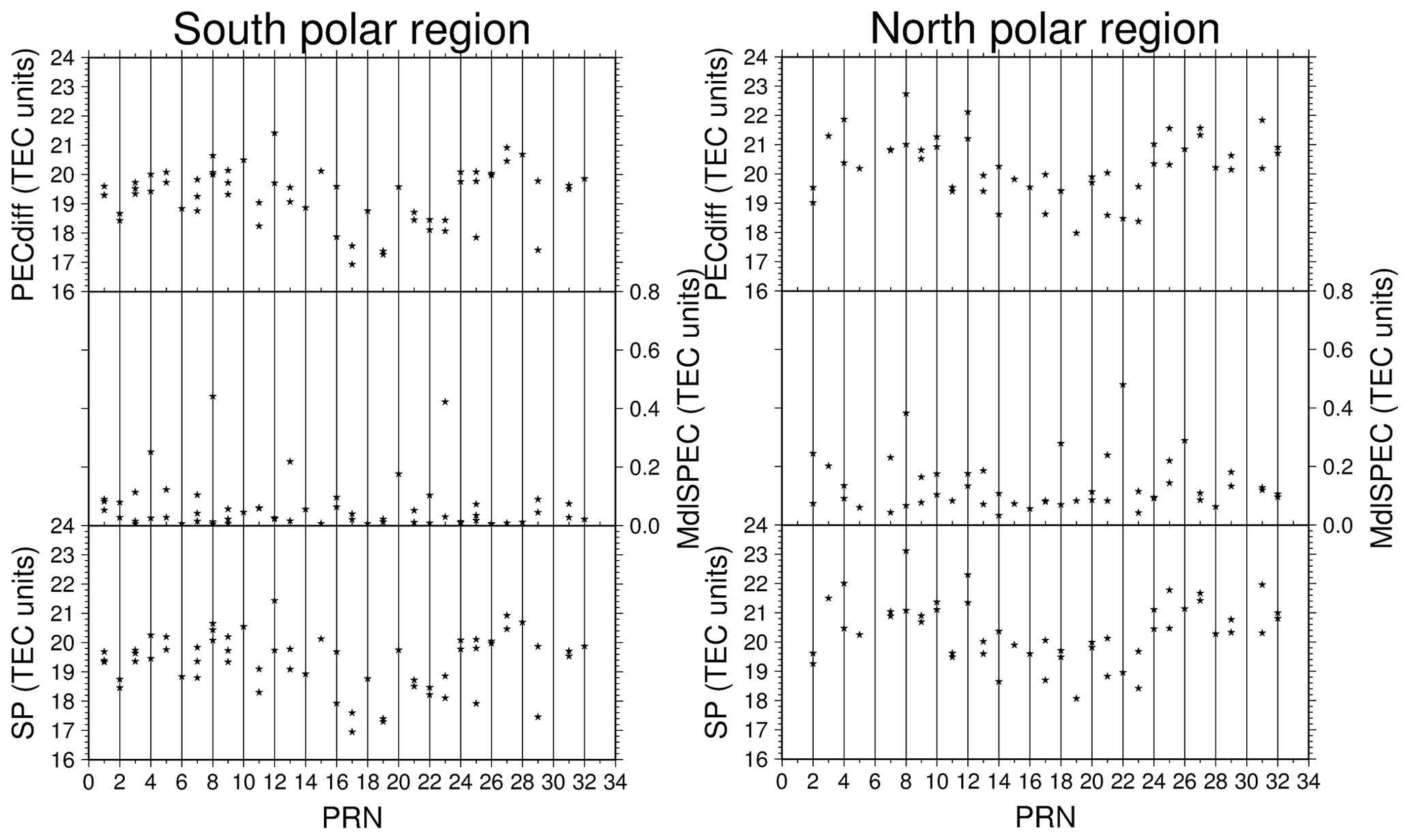
Figure 3 Comparisons of minimum Jason-2 uncalibrated GPS SPEC (SP) values with minimum PIM SPEC (MdlSPEC) for contiguous GPS satellite segments in each polar region, with the corresponding differences $\text{PECdiff}=\text{SP}-\text{MdlSPEC}$, for each GPS PRN number.

All of the contiguous GPS satellite segments observed by the Jason-2 receiver were surveyed for possible SPEC values smaller than that measured for the polar regions. One short (8 min), low-elevation (below 7^∘) segment for PRN 19 was noted, with SPEC values near 14 TEC units. However, the estimated error for the alignment of the SP and SR values was about 0.9 TEC units, so this minimum SP was not considered reliable, and this data segment was excluded. The derived receiver bias value was then applied to all of the remaining Jason-2 satellite SPEC data.

An assessment of the receiver bias error was performed through examination of the cumulative distribution of derived SPEC values. Figure 4a displays the cumulative distribution of SPEC values calculated from PIM. The sharp increase in the distribution for SPEC values near zero indicates a high percentage of SPEC occurrences within a small range of SPEC values ($\mathrm{0}\le \text{SPEC}\le \mathrm{0.2}$). However, if there are measurement errors larger than 0.2 TEC units associated with SPEC values, this small SPEC range could not arise. This is illustrated in Fig. 4b, for which Gaussian “noise” with a standard deviation of 0.75 TEC units is added to the data set. The low-SPEC end of the cumulative distribution then has a more gradual increase, which closely resembles the low-SPEC end of the actual SPEC cumulative distribution, displayed in Fig. 4c. Detailed characteristics of the low end of the cumulative distribution vary, depending on the standard deviation of the noise, so the value of 0.75 TEC units was chosen as the closest match from a set of comparisons. This value was designated as the initial error for the Jason-2 receiver bias. Because the actual low-SPEC end of the cumulative distribution is unlikely to be so steep, arising from a sharp high-latitude plasmapause limit and a limited ionosphere extension, the estimate for the SPEC error is a probable upper bound. It is noteworthy that this error estimate is larger than the typical error range of 0.1–0.3 TEC units arising from the alignment of the SP values to the SR values, which is one of the sources contributing to this error.

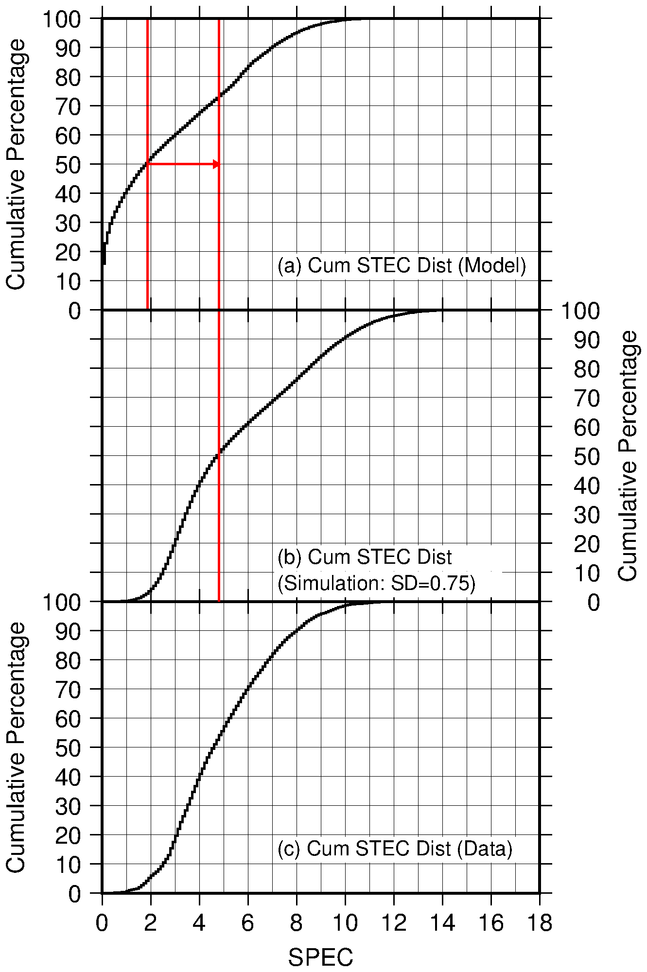
Figure 4 Cumulative distributions for the slant PEC (SPEC) values (in TEC units) from (a) PIM (for the same lines of sight as the data samples); (b) PIM, with added Gaussian noise, having a standard deviation of 0.75 TEC units; and (c) measured, calibrated SPEC data. The vertical red lines indicate the shift of the median of the cumulative distribution for the PIM values, induced by the noise tail at the low end of the distribution.

A distinct feature occurring between the two simulation panels (Fig. 4a and b) is the shift of the median value for the cumulative distribution, indicated by the two red lines, arising from the noise tail at the low end of the distribution and especially from the lowest value in the noise tail. To evaluate this effect, simulations were performed for 25 separate cases of added noise, all from Gaussian distributions with a standard deviation of 0.75 TEC units. For these cases, the median value of the distribution shifts was 2.962 TEC units, the mean value of the distribution shifts was 2.986 TEC units, and the standard deviation of the distribution shifts was 0.181 TEC units (for a distinctly non-Gaussian distribution of shift values). The median value of the distribution shifts (2.962) was used for the bias adjustment rather than the mean value (2.986) because of this non-Gaussian distribution of shift values, producing a revised bias value of 19.890 TEC units. The standard deviation of the distribution shifts was combined with the noise standard deviation to give an estimated bias error of 0.772 TEC units. After this bias correction is applied, 16.8 % of Jason-2 slant PEC values are negative, and the revised cumulative distribution median value is 1.66 TEC units.

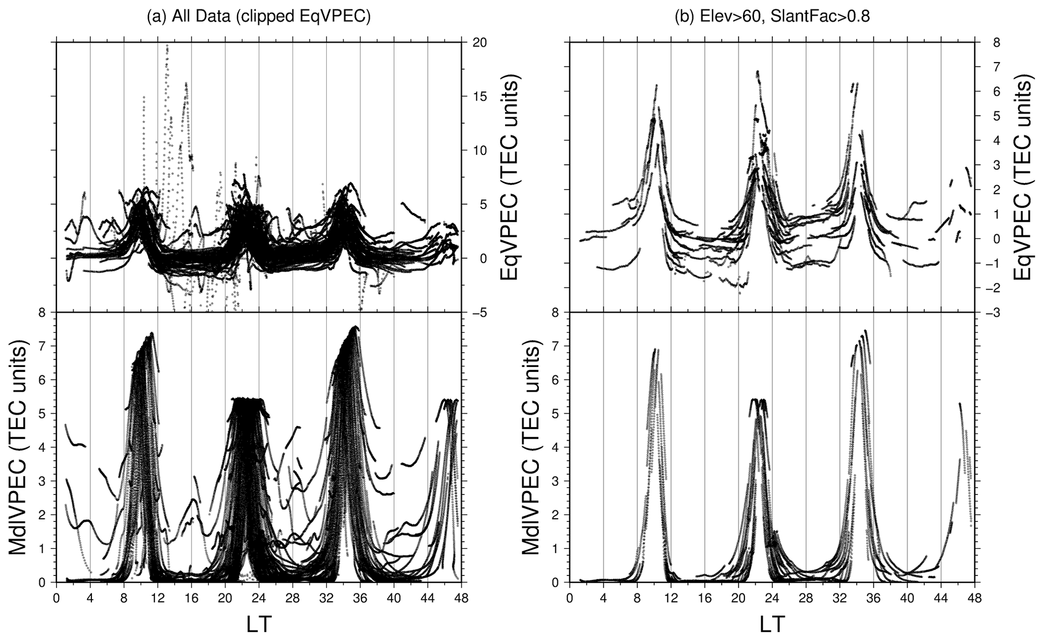
Figure 5 (a) PIM VPEC (MdlVPEC) and equivalent vertical measured PEC (EqVPEC) versus local time (LT) for all data samples (display limited from −5 TEC units for EqVPEC). The minimum EqVPEC value is nearly −36 TEC units, arising from small values for the ratio (SlantFac) of model slant PEC (MdlSPEC) to model equivalent vertical PEC (MdlVPEC). (b) MdlVPEC and EqVPEC versus LT for data subset, selected by $\mathrm{60}{}^{\circ }\le \text{Elevation}\le \mathrm{90}{}^{\circ }$ and 0.8≤SlantFac.

For 11 of the simulation cases, the cumulative distributions for the simulated data have median values near those of the actual data, after the minimum SPEC bias correction is applied (as in Fig. 4c). For the same simulation cases, the noise tails at the low end of the distributions also match the low end of the data distribution. Thus, the calibration could have been accomplished by determining the difference between the median for the original data (without the preliminary adjustment based on the polar region values) and the median for the original model values (as in Fig. 4a, without the simulated noise). If an alternative error estimate is available for the bias, the determination of the noise standard deviation and the associated noise simulations for the model data could be omitted. However, this would also eliminate the verification of matching the low end of the data cumulative distribution and omit a small correction for the variation of the simulated data median values among cases.

An alternative statistical bias determination is described by Heise et al. (2005), utilizing an average of the differences between measured and model values to evaluate the bias, for a high-latitude subset of the data. For the combined high-latitude data sets selected in this study, their method produces a bias value of 19.846 ± 1.042 TEC units.

A somewhat different method, the “Improved ZERO TEC Method”, is described by Zhong et al. (2016), consisting of a daily determination and a correction derived from all days of data. Because only 1 d of data is analyzed here, only the first part of their evaluation could be applied, involving the minimum SPEC for individual ascending and descending orbital legs. From that evaluation, using the smaller first quartile of the two sets (ascending, descending) of SPEC values, the derived bias shift was 0.618 TEC units, relative to the provisional assignment of 16.928 TEC units. This is significantly less than the value derived above for the median shift, and this result was not used.

Two other calibration methods, the minimum standard deviation method (Valladares et al., 2009) and the SCORE method (Bishop et al., 1994), adapted from ground-based methods, were examined but not used for the data analysis. A description of these evaluations is provided in the Supplement.

Because of the low ion density of the plasmasphere, relative to even the topside ionosphere, and the significant variation of the plasmapause altitude with latitude, the designation of a representative altitude for the usual thin-shell formula converting from slant TEC to equivalent vertical TEC was considered problematic (e.g., Mazzella, 2009, Fig. 5 and Eq. 1). Rather than attempting to develop and implement a different formula for the conversion between SPEC and VPEC for all the data, accounting for the satellite altitude and latitude, as well as the azimuth and elevation of the line of sight, PIM was utilized to accomplish this conversion. The PIM SPEC (MdlSPEC) was calculated for all data samples, based on the Jason-2 location and the time, elevation, and azimuth of each of the lines of sight. For each sample, the median altitude (MedAlt) for the cumulative slant PEC profile versus altitude was also evaluated. The associated latitude (MedLat) and longitude (MedLong) for the median-altitude occurrence were then determined. The corresponding model vertical PEC (MdlVPEC) was calculated for the (MedLat, MedLong) location, and a representative equivalent vertical PEC for each data sample (EqVPEC) was calculated as

$$\begin{array}{}\text{(3)}& \text{EqVPEC}=\text{SPcal}\cdot \left({\displaystyle \frac{\text{MdlVPEC}}{\text{MdlSPEC}}}\right),\end{array}$$

where SPcal is the calibrated GPS SPEC. All of these results were reviewed graphically.

A composite plot for all data is displayed in Fig. 5a for both the MdlVPEC and EqVPEC versus local time (LT) at the median-altitude location. A [0,24] h limit is not imposed on the LT evaluations, and continuity in LT is maintained for successive GPS samples, except for the (positive East) longitude discontinuity from 360 to 0^∘ in each orbit. Thus, for the combined universal time (UT) and longitude (Long) progressions (with $\text{LT}\left(\mathrm{h}\right)=\text{UT}\left(\mathrm{h}\right)+\text{Long}\left({}^{\circ }\right)/\left(\mathrm{15}{}^{\circ }{\mathrm{h}}^{-\mathrm{1}}\right)$), the LT values extend over [0,48] h for the 24 h of universal time. The MdlVPEC values display a day/night difference that appears to be absent for the derived EqVPEC results, and the EqVPEC results display many anomalous values. These values are associated with MdlSPEC $/$ MdlVPEC (slant factor) values below 0.8. Consequently, a selected subset of the data was chosen and is displayed in Fig. 5b, with the selection criteria being as follows:

• $-\mathrm{65}{}^{\circ }\le \text{MedLat}\le \mathrm{65}{}^{\circ }$,

• $\mathrm{60}{}^{\circ }\le \text{Elevation}\le \mathrm{90}{}^{\circ }$,

• 0.8≤SlantFac (≡ MdlSPEC $/$ MdlVPEC).

Note that for these selection criteria, the day/night difference is still absent for the measured EqVPEC.

3 Comparisons over Africa

For comparison with the previous ground-based study for Africa, a preliminary regional survey was performed for the following parameter selections:

• $-\mathrm{60}{}^{\circ }\le \text{MedLat}\le \mathrm{40}{}^{\circ }$,

• $-\mathrm{10}{}^{\circ }\le \text{MedLong}\le \mathrm{75}{}^{\circ }$,

• $\mathrm{60}{}^{\circ }\le \text{Elevation}\le \mathrm{90}{}^{\circ }$,

• 0.8≤SlantFac.

These results are displayed in Fig. 6 for the Jason-2 tracks in the vicinity of Africa (in red) and the associated median-altitude occurrences for lines of sight to the GPS satellites (in blue). The rings around the displayed subset of sites correspond to a (ground-based) threshold elevation of 35^∘, intersecting the Jason-2 altitude (1346 km), for the inner ring and a representative median altitude (3173 km) for the cumulative line-of-sight slant PEC (as determined from PIM) for the outer ring. Only the Jason-2 line-of-sight median-altitude occurrences (blue) within the outer ring for a station are suitable for vertical PEC comparisons for that station. (Note that not all of the stations in the Africa chain are displayed, to avoid confusion among the rings, but the subset that is displayed reasonably represents the regional coverage of all of the stations.)

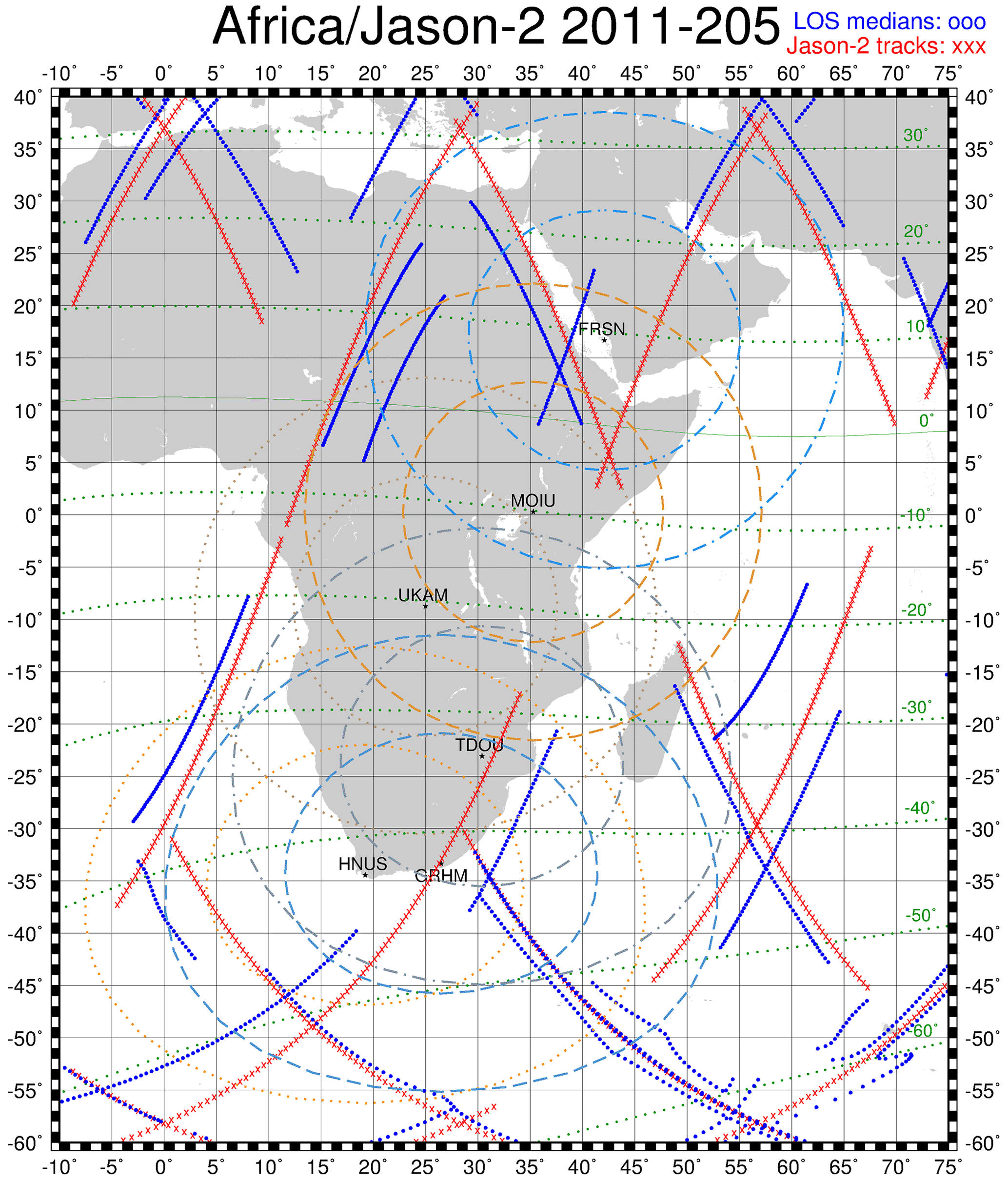
Figure 6 Comparison of Jason-2 coverage with coverage by a representative subset of the ground-based sites for the previous Africa chain study (day 205, 2011) (Mazzella et al., 2017). The Jason-2 tracks in the vicinity of Africa are displayed as red tracks (×), and the associated median-altitude occurrences for lines of sight (LOSs) to the GPS satellites are displayed as blue segments (∘). The rings around the displayed subset of sites correspond to a threshold elevation of 35^∘, intersecting the Jason-2 altitude for the inner ring and a representative median altitude for the cumulative line-of-sight slant PEC for the outer ring. The magnetic latitudes displayed within the plot frame are magnetic apex coordinates (VanZandt et al., 1972), calculated for consistency with the ground station locations.

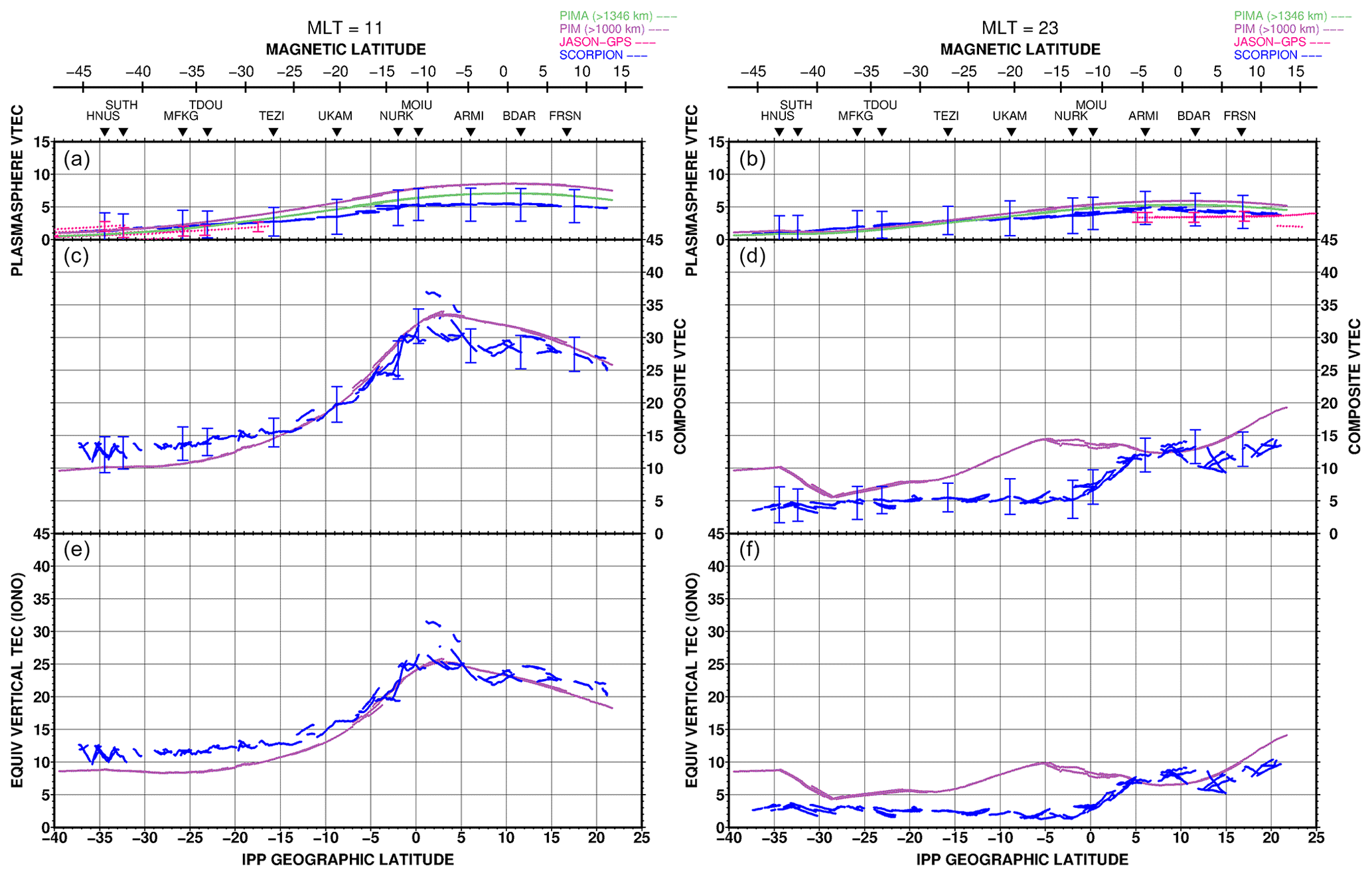
Figure 7 Latitudinal vertical TEC profiles (in TEC units) separately for the ionosphere (e, f) and plasmasphere (a, b) (for an ionosphere–plasmasphere boundary at 1000 km), with the composite (ionosphere plus plasmasphere) vertical TEC (c, d), for the SCORPION and PIM results and for the plasmasphere only for the Jason-2 results (with a base altitude of 1346 km) for magnetic local times 11:00 (a, c, e) and 23:00 (b, d, f). The corresponding PIM profiles are displayed for a 1000 km boundary for the ionosphere only (e, f) and as the upper PIM profile (“PIM (>1000 km)”) for the plasmasphere, while the lower PIM plasmasphere profile (“PIMA (>1346 km)”) corresponds to an alternative boundary altitude of 1346 km for comparison with the Jason-2 values.

Table 1 The sites used for the Africa chain study, plus the auxiliary sites Kerguelen Islands and Grahamstown (officially known as Makhanda), from south to north, with their supporting networks and their derived plasmasphere baseline values (in TEC units) (Mazzella et al., 2017).

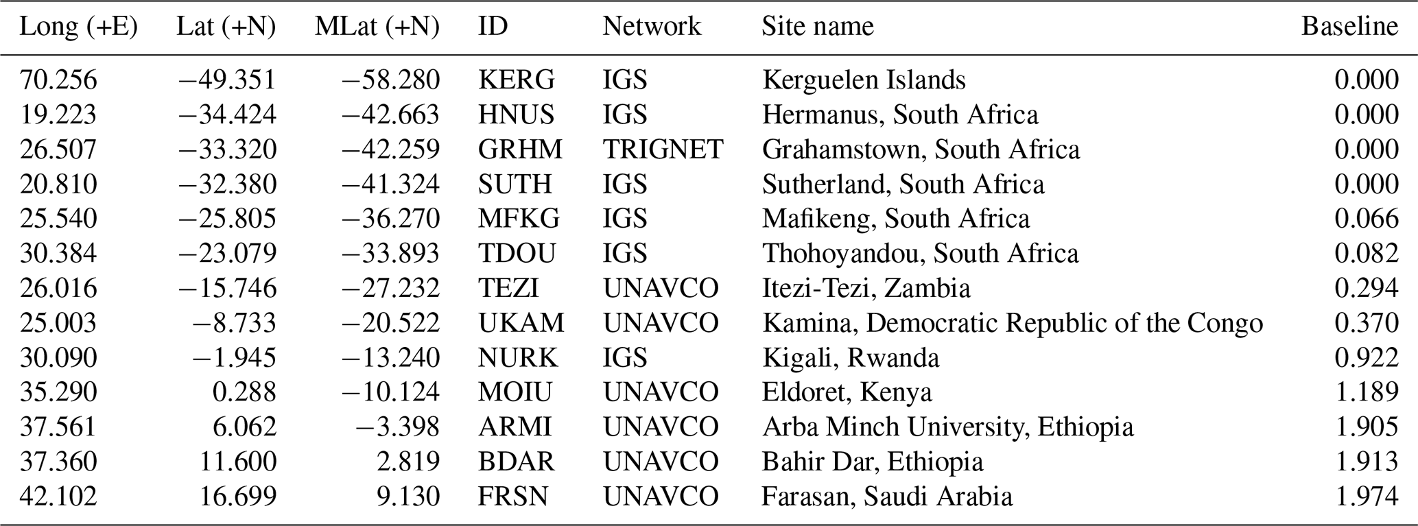
Because of the high inclination (66.04^∘) of the Jason-2 orbit, the satellite passages over Africa occur primarily for magnetic local times around 11:00 (for southward passages) and 23:00 (for northward passages) for this day, using the ground station magnetic local time (MLT) selection conventions previously employed by Mazzella et al. (2017). Data for these two periods, within a half-hour of the nominal magnetic local times, were selected for both the Jason-2 GPS data and the GPS data for each of the ground stations used for the African chain, which are listed in Table 1 (Mazzella et al., 2017), together with their plasmasphere baseline values, in TEC units. Jason-2 equivalent vertical PEC (EqVPEC) and ground-station plasmasphere vertical electron content (VPEC) derived by the SCORPION method are displayed in Fig. 7 (top panels) as latitudinal profiles, together with the ionosphere vertical electron content (bottom panels) and composite ionosphere and plasmasphere vertical electron content (middle panels) derived by SCORPION. The error bars in Fig. 7 for the ground-based TEC measurements are calculated in the manner described by Mazzella et al. (2017), while the Jason-2 TEC error bars are derived from the analysis for Fig. 4, based on the Gaussian noise (0.75 TEC units) required to reproduce the cumulative distribution for the Jason-2 TEC data. The Jason-2 EqVPEC values are less than the corresponding SCORPION VPEC values, by 0.82 ± 0.28 TEC units, at both high latitudes (daytime samples) and low latitudes (nighttime samples). Because the Jason-2 satellite altitude (1346 km) is greater than that of the nominal ionosphere–plasmasphere boundary (1000 km) used for SCORPION, the Jason-2 EqVPEC is expected to be slightly less than the SCORPION VPEC. From plasmasphere electron content calculated from the PIM/Gallagher model, the vertical PEC between 1000 and 1346 km ranges from 0.59 to 1.50 TEC units for the daytime period (versus 0.75 ± 0.18 TEC units for SCORPION minus Jason-2) and 0.26 to 0.62 TEC units for the nighttime period (versus 0.91 ± 0.35 TEC units for SCORPION minus Jason-2). The intrinsic VPEC variation determined by SCORPION between the two magnetic local times, for latitude ranges corresponding to the respective Jason-2 latitudes, is 2.35 ± 0.59 TEC units.

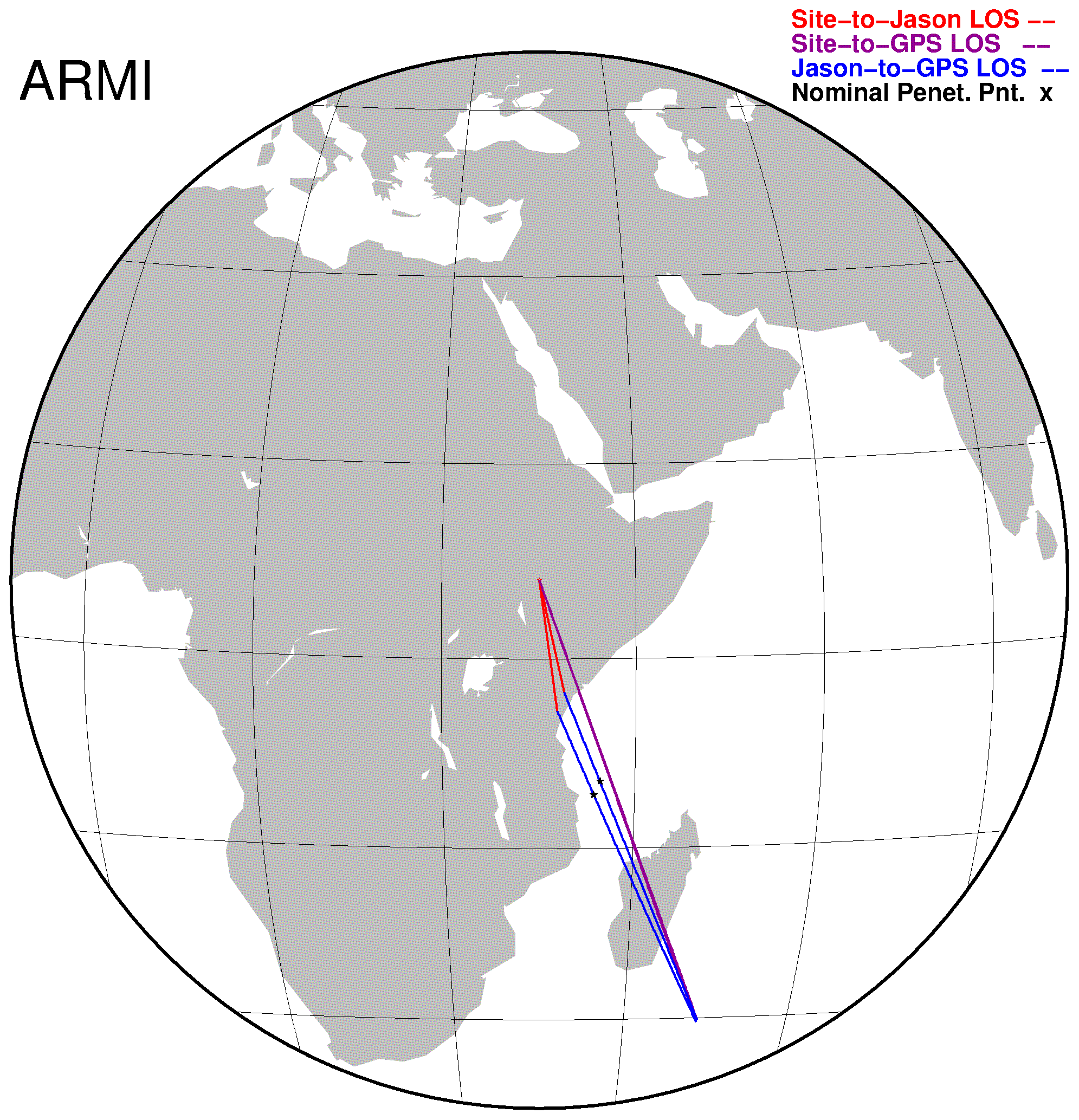
Figure 8 Aligned lines of sight from the ground station ARMI to Jason-2 (red) and to the common GPS satellite (PRN 14) observed (purple), plus the lines of sight (blue) from Jason-2 to that GPS satellite, with nominal plasmasphere penetration points for the Jason-2 lines of sight (black dots), based on the median cumulative slant TEC calculated from PIM. The ground-based elevation of the GPS satellite for the occurrences displayed is about 41^∘.

An alternative survey was conducted for Jason-2 data in the vicinity of the ground-based GPS stations, using only the elevation threshold, without the slant factor restrictions associated with Fig. 6. The objective of this survey was to find aligned line-of-sight occurrences, for the same GPS satellite, for Jason-2 paired with each of the ground stations so that the corresponding SPEC measurements could be compared, obviating the requirement for slant-to-vertical conversions for the PEC measurements. The alignment was quantified using the angle between the Jason-2 line of sight to the GPS satellite and the ground-based line of sight to Jason-2, measured at Jason-2. The angular limit for selection of these occurrences was set as 10^∘, with a ground-based elevation threshold for Jason-2 designated as 35^∘. Like the comparison of equivalent vertical PEC measurements, the ground-based SPEC measurements were expected to be slightly larger than the Jason-2 SPEC measurements.

There were two to four ground-based/Jason-2 matches for most of the sites listed in Table 1, with no matches for GRHM and only one for KERG, although as many as three of the matches at a site could be distinct Jason-2 occurrences for nearly coincident ground-based observations of a single GPS satellite. There were a total of 32 matches for the 10^∘ alignment limit, with the minimum GPS elevation observed by Jason-2 being about 37^∘ and the minimum ground-based GPS satellite elevation being about 32^∘.

An example of alignments for the ground station ARMI is displayed in Fig. 8, indicating the lines of sight from the station to Jason-2 (red) and the common GPS satellite (PRN 14) (purple), plus the lines of sight from Jason-2 to that GPS satellite (blue). Nominal plasmasphere penetration points for these Jason-2 lines of sight are indicated (black dots), based on the median cumulative slant TEC calculated from PIM, showing the distance of these penetration points from the location of Jason-2 and the assigned location for the EqVPEC (although the EqVPEC is not used in this comparison). The two cases displayed are the only two alignments for ARMI for day 205, 2011, at the 30 s sampling of the ground station GPS data. (The two distinct GPS satellite locations are nearly coincident, and redundant pairings associated with the 10 s Jason-2 data sampling are not utilized.)

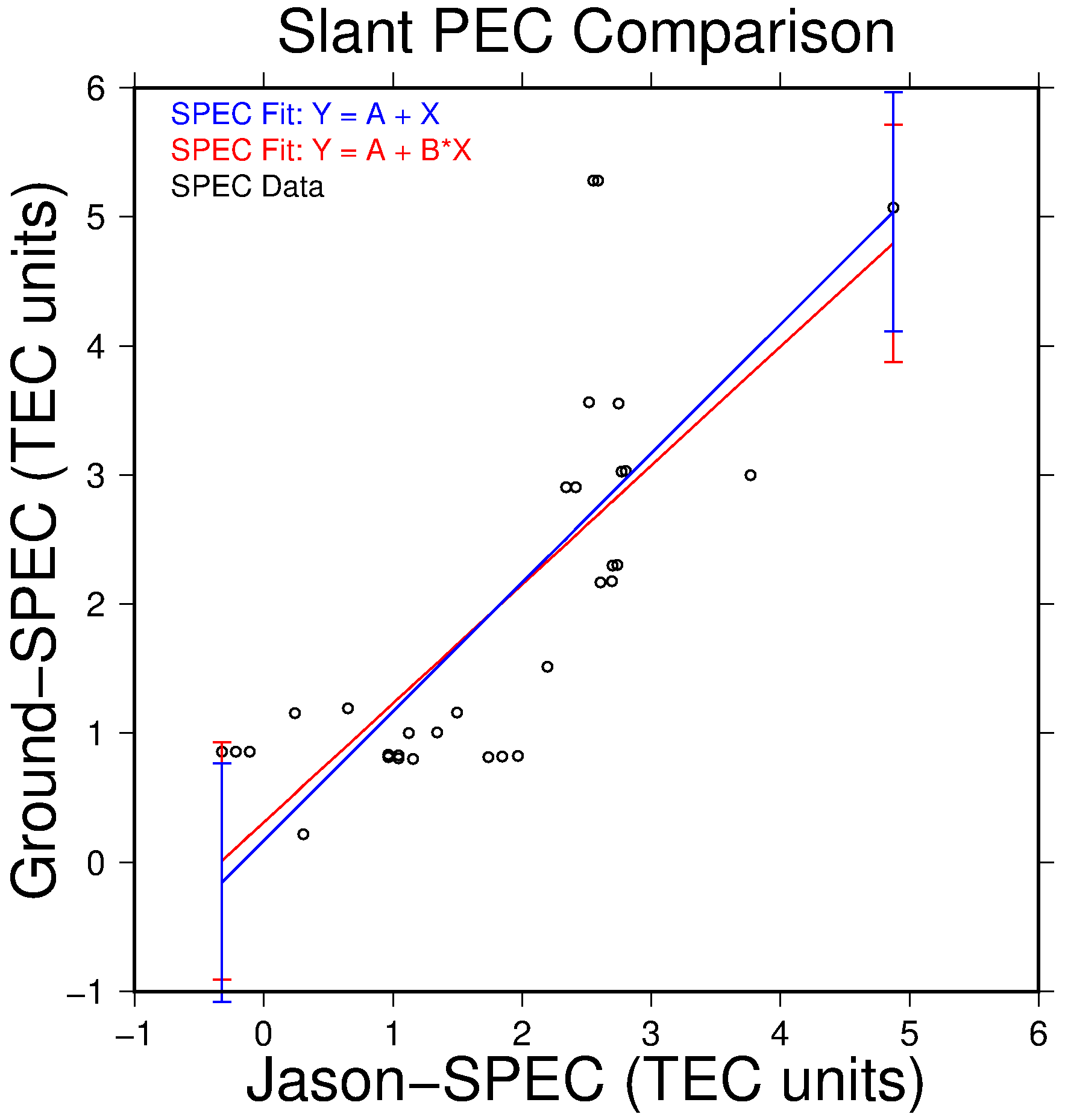
Figure 9 SPEC comparisons for ground-based GPS receivers (Ground–SPEC) versus the Jason-2 GPS receiver (Jason–SPEC) (circles), with two alternative linear fits: ($Y=A+X$) (blue) and ($Y=A+B\cdot X$) (red), both indicating intercepts of about 0.24 TEC units.

For all of the sites, the SPEC comparisons arising from the alignment cases are displayed in Fig. 9 (circles), showing slightly higher SPEC values for the SCORPION ground-based measurements by about 0.24 TEC units. For comparison, an offset linear fit ($Y=A+X$) to the data samples, with an intercept of 0.168 ± 0.924 TEC units, is displayed in blue, and a first-order fit ($Y=A+B\cdot X$), with a slope of 0.921 and an intercept of 0.311 ± 0.920 TEC units, is displayed in red. A tabulation of all the SPEC comparisons and associated parameters is provided in the Supplement, as the data for Fig. 9.

4 Discussion and conclusions

This study supplements a previous analysis of ground-based GPS TEC measurements over Africa (Mazzella et al., 2017), specifically for comparison of the plasmasphere component of those measurements, by analyzing GPS measurements from a Jason-2 satellite-borne receiver, thus intrinsically isolating the plasmasphere contribution. The comparisons were conducted for both the derived EqVPEC determination, which is a secondary quantity produced using several underlying assumptions and conversions, and the SPEC determination, which is a more directly derived quantity, especially for the Jason-2 measurements. The Jason-2 measurements are affected primarily by the receiver bias determination but also by the relative biases for the individual GPS satellites. This comparison of satellite-based SPEC to ground-based SPEC measurements may be the first such comparison reported or conducted.

In addition to the derived Jason-2 receiver bias, the EqVPEC determinations from Jason-2 rely on the relative GPS satellite biases and the conversion of the SPEC measurements to representative EqVPEC values. As noted above, the assessments for the satellite bias for PRN 1 changed significantly (by about 7.6 TEC units) between the July 2011 and August 2011 tabulations by CODE, with the August 2011 value being more consistent with the values derived for the African stations by the SCORPION method for 24 July 2011 (Mazzella et al., 2017, Fig. 8). In this case, the July 2011 PRN-1 bias was underestimated, but an overestimate of the same magnitude would have resulted in the PRN-1 SP values in Fig. 3 becoming the lowest measured SP values and thus affecting the initial evaluation for the Jason-2 receiver bias (prior to the adjustment for the median shift). However, all of the PRN-1, high-latitude SP values in Fig. 3 would be distinct outliers for such an occurrence and thus subject to further examination and likely elimination.

The PIM/Gallagher (Daniell et al., 1995; Gallagher et al., 1988) ionosphere–plasmasphere model was used to provide both correction values for the Jason-2 receiver bias determination and slant factors for the conversion from SPEC to EqVPEC for the satellite-based measurements. While some erratic slant factor values (attributed to small MdlSPEC and MdlVPEC values) arose from this process, the oversimplification of a single reference slant factor altitude was circumvented.

For differences taken as ground-based minus Jason-2 measurements, the mean difference for vertical PEC comparisons is 0.82 ± 0.28 TEC units, while the mean difference for SPEC comparisons is 0.168 ± 0.924 TEC units. The large error designated for the SPEC comparisons reflects the small sample count for the comparison pairs and some significant outliers.

The Jason-2 SPEC comparison method may provide a reliable value for the plasmasphere baseline determination for the ground-based receivers, especially if the ground stations are confined to only midlatitude or low-latitude regions. For these regions, the plasmasphere can provide an apparent spatially constant (over the sky regions above the observational elevation threshold) and temporally constant (over the generally 1 d observation period) contribution that can be mistaken as a bias component. The Jason-2 satellite, by sampling high-latitude regions with essentially zero plasmasphere electron content, can provide an alternative reference for the baseline ambiguity of the ground-based plasmasphere measurements. This expectation is supported by the close agreement, in Fig. 9, of the offset linear fit to the more general first-order linear fit. However, the applicability of this reference usage is slightly degraded by the difference in the altitudes used by Jason-2 and the ground-based measurements for the plasmasphere lower boundary and the relatively large error bars compared to the tabulated plasmasphere baseline values (Table 1).

With regard to the PIM/Gallagher model, a generally good agreement is obtained with both the Jason-2 and SCORPION vertical PEC results for the nighttime case (Fig. 7, MLT=23), although the Jason-2 measurements are confined to the magnetic equatorial region for this case. The PIM/Gallagher results are also consistent with the Jason-2 and SCORPION vertical PEC results for the high-latitude region for the daytime case (Fig. 7, MLT=11) but diverge from the SCORPION results at low latitudes. A notable difference between the vertical PEC results for PIM/Gallagher and either Jason-2 or SCORPION is the diminished equatorial day/night variation obtained by Jason-2 (Fig. 5) and SCORPION (Fig. 7). (This is further evident for SCORPION from Figs. 4 and 5 by Mazzella et al., 2017.) A similar small day/night variation (about 1 TEC unit) was noted by Lee et al. (2013) for a multi-year study (2002–2009).