Effects of the terdiurnal tide on the sporadic E (E_s) layer development at low latitudes over the Brazilian sector

Sporadic E (E_s) layers are patches of high ionization observed at around 100–140 km height in the E region. Their formation at low latitudes is primarily associated with the diurnal and semidiurnal components of the tidal winds via the ion convergence driven by the wind shear mechanism. However, recent studies have shown the influence of other tidal modes, such as the terdiurnal tide. Therefore, this work investigates the effect of terdiurnal tide-like oscillations on the occurrence and formation of the E_s layers observed over Palmas (10.17^∘ S, 48.33^∘ W; dip lat. −7.31^∘), a low-latitude station in Brazil. The analysis was conducted from December 2008 to November 2009 by using data collected from CADI (Canadian Advanced Digital Ionosonde). Additionally, the E Region Ionospheric Model (MIRE) was used to simulate the terdiurnal tidal component in the E_s layer development. The results show modulations of 8 h periods on the occurrence rates of the E_s layers during all seasonal periods. In general, we see three well-defined peaks in a superimposed summation of the E_s layer types per hour in summer and autumn. We also observed that the amplitude modulation of the terdiurnal tide on the E_s occurrence rates minimizes in December in comparison to the other months of the summer season. Other relevant aspects of the observations, with complementary statistical and periodogram analysis, are highlighted and discussed.

1 Introduction

Sporadic E (E_s) layers are thin and dense layers observed in the ionospheric E region at altitudes ranging from 100 to 140 km. The ion density of the E_s layer is associated with molecular ions, mostly O${}_{\mathrm{2}}^{+}$ and NO⁺, and the main metal ions Fe⁺, Mg⁺, and Na⁺. Metal ions have a longer lifetime than the molecular ions, making the E_s layers long-lasting (Whitehead, 1989; Plane, 2003).

The E_s layers are divided into three different classes: equatorial layers, low- and mid-latitude layers, and the auroral or high-latitude layers. They are differentiated into types designated by the lowercase letters of the alphabet, such as E${}_{{\mathrm{s}}_{\mathrm{c}}}$ (cusp), E${}_{{\mathrm{s}}_{\mathrm{f}}}$ (flat), E${}_{{\mathrm{s}}_{\mathrm{h}}}$ (high), E${}_{{\mathrm{s}}_{\mathrm{l}}}$ (low), E${}_{{\mathrm{s}}_{\mathrm{q}}}$ (equatorial), E${}_{{\mathrm{s}}_{\mathrm{a}}}$ (auroral), and E${}_{{\mathrm{s}}_{\mathrm{s}}}$ (slant). The “c”, “h”, “l”, and “q” types are formed in the daytime, while the “f” type is usually nocturnal. Type “h” of E_s occurs at higher altitudes, generally ranging between 120 and 140 km, and it can appear and disappear suddenly, as well as evolving into type “c” at lower altitudes (Conceição-Santos et al., 2020). The “l” and “f” types generally occur at 100–110 km. Furthermore, the “q” type occurs near the magnetic equator around 100 km (Resende et al., 2017b; Conceição-Santos et al., 2020).

The E_s layers occur at most latitudes and longitudes and have different mechanisms of formation that depend mainly on magnetic latitude (Kirkwood and Nilsson, 2000). The vertical shear in the east–west component of horizontal winds (wind shear) is the most accepted theory to explain the formation of E_s layers. According to this theory, a vertical convergence of the charged particles occurs by U×B forces, where U and B denote the horizontal wind and the Earth's geomagnetic field, respectively (Whitehead, 1961, 1989; Kirkwood and Nilsson, 2000; Haldoupis, 2012). The atmospheric tides are one of the possible sources of wind shears, which means that solar tides can strongly control the intensification of E_s layers (Forbes and Wu, 2006; Forbes et al., 2008; Moudden and Forbes, 2013). Solar tides are oscillations in the atmosphere that occur due to the absorption of infrared and EUV (extreme ultraviolet) radiation by water (H₂O), ozone (O₃), and molecular oxygen (O₂) in the troposphere, stratosphere, and lower thermosphere. This absorption of radiation causes periodic heating and expansion of tidal amplitudes that grow exponentially in height as they are excited into regions of the lower thermosphere between the altitudes of 90 and 120 km (Forbes and Wu, 2006; Forbes et al., 2008; Smith, 2012; Pancheva et al., 2013).

The source of terdiurnal tide generation has two main discussions currently in the literature, one being the nonlinear interaction between the diurnal and semidiurnal tides (Teitelbaum and Vial, 1991; Huang et al., 2007; Forbes and Wu, 2006; Forbes et al., 2008; Truskowski et al., 2014; Forbes et al., 2014), and the other is direct solar heating (Akmaev, 2001; Smith and Ortland, 2001; Du and Ward, 2010; Lilienthal and Jacobi, 2019). For Truskowski et al. (2014), the terdiurnal tide is generated by the nonlinear interaction between the diurnal and semidiurnal tides at mid- and low-latitude regions, but they did not rule out the contribution of direct warming. Lilienthal and Jacobi (2019) showed that direct heating is the primary source of terdiurnal tide generation at mid- and low-latitude regions in the Northern Hemisphere and Southern Hemisphere, with nonlinear interaction being a secondary source. The seasonality of the terdiurnal tidal amplitude has been studied in the interest of understanding its source of generation and its variability in the lower thermosphere, which can have maxima in different months and latitudes of the hemispheres (Zhao et al., 2005; Jiang et al., 2009; Venkateswara Rao et al., 2011; Moudden and Forbes, 2013; Fytterer et al., 2014; Jacobi and Arras, 2019).

The phase and vertical wavelength of the terdiurnal tide vary as a function of season and latitude and differ between the zonal and meridional components (Zhao et al., 2005; Venkateswara Rao et al., 2011; Jacobi and Arras, 2019). Jacobi and Arras (2019) compared data results between the Collm (51^∘ N) and Obninsk (55^∘ N) meteoric radars, showing the variability of tidal amplitudes between seasons, but the annual seasonal cycles were approximately the same for the zonal and meridional components at these latitudes. Moudden and Forbes (2013) also found periodic seasonality of the terdiurnal tide at mid- and low-latitude regions when they focused their analyses on the TW3, TE1, TW4, and TW5 (terdiurnal tides for east (TE) and west (TW) with zonal numbers 1, 3, 4, and 5) to try answering why these tides have well-defined and repeatable seasonal behaviors from year to year in the Northern Hemisphere and Southern Hemisphere. The authors pointed out that the TW3 tide has the greatest amplitude near the magnetic equator in both hemispheres and has two distinct peaks that occur regularly each year above 110 km on the autumn and spring equinoxes and in the month of February. According to the authors, this tide showed similar characteristics to diurnal tide (DW1) and semidiurnal tide (SW2) with respect to annual periodicity and seasonal variability of amplitude in the latitudes of the two hemispheres. Fytterer et al. (2014) analyzed the effect of the terdiurnal tide on the frequencies (foE_s) of E_s layers using radio occultation (RO) data over a global distribution between ± 60^∘, revealing nearly uniform numbers of E_s layer occurrences and terdiurnal tide amplitude across years at latitudes in both hemispheres. The authors used the months of January and April, respectively, as representative of the summer solstice and autumn equinox, observing good agreement between the terdiurnal amplitude and the occurrences of E_s layers with 8 h shear characteristics. Jacobi and Arras (2019) analyzed the diurnal, semidiurnal, and terdiurnal tidal phases over the E_s layers using 1 year as representative of a seasonal tidal cycle. The authors concluded that the tides observed in the E_s layers are largely due to neutral zonal wind shear in the presence of a component of the Earth's magnetic field. Tidal winds maintain a certain annual periodicity across latitudes (Moudden and Forbes, 2013; Fytterer et al., 2014; Jacobi et al., 2017; Jacobi and Arras, 2019) so that a 1-month analysis can represent the tide in a season and a 1-year analysis can represent a tidal cycle at a given latitude in the hemispheres. It is worth mentioning that this work is restricted to presenting a possible effect of the terdiurnal tide on the E_s layer formation, and it is not concerned with the behavior of the terdiurnal tide.

The type of atmospheric tide can influence the development of the sporadic layers (Haldoupis and Pancheva, 2006; Haldoupis, 2012; Lilienthal et al., 2018). The convergence of the E_s layer to altitudes whose vertical velocities of neutral winds correspond to zero may be driven by the global tidal wind system in the thermosphere (Haldoupis, 2012). The formation and variability of the E_s layers may be related to the action of atmospheric waves in the lower thermosphere (McLandress, 2002a, b; Haldoupis and Pancheva, 2006; Haldoupis, 2012). Haldoupis et al. (2004) used a time series of E_s layer parameters scaled from ionosonde data and found that the dominant amplitudes at the 3 to 36 h period are the 24, 12, and 8 h peaks associated, respectively, with the diurnal, semidiurnal, and terdiurnal atmospheric tides. Although the diurnal and semidiurnal tides play leading roles in the occurrence, altitude descent, and strength of E_s layers, Haldoupis and Pancheva (2006) stressed that the terdiurnal tide can also have a contribution to the convergent shearing of the horizontal winds. In the mid-latitude station of Cyprus (35.0^∘ N, 33.0^∘ E), Oikonomou et al. (2014) observed the presence of terdiurnal tidal effects on the E_s layer that prevailed only during summer months.

Additionally, Fytterer et al. (2014) used an atmospheric circulation model to support the observations of GPS radio occultation data, and the authors reported a well-pronounced peak in the E_s layer occurrence at around 10^∘ in both hemispheres associated with the migrating terdiurnal tide. In the Brazilian sector, Resende et al. (2016) and Resende et al. (2017a, b) simulated the E_s layer using a model called MIRE (E Region Ionospheric Model). They showed that the diurnal and semidiurnal components are the main ones for forming the E_s layer in this sector. However, they suggested that some discrepancies between the model and observational data might be due to the exclusion in the analysis of other tidal components such as terdiurnal and quarter-diurnal tides. It is worth mentioning that there are few studies in the literature concerning the role of the terdiurnal tidal modulation in the formation of E_s layers, especially in equatorial and low-latitude regions (Haldoupis and Pancheva, 2006; Fytterer et al., 2014; Lilienthal et al., 2018).

Although our knowledge of tidal effects on E_s layers has advanced over the last 20 years, there are still questions about the possible role of the terdiurnal tide on the formation of E_s layers at low latitudes. Therefore, the present study analyzes the E_s layer parameters obtained from ionosonde data from an instrument installed in the low-latitude station of Palmas, Brazil (10.17^∘ S, 48.33^∘ W; dip lat. −7.31), to investigate the modulation of the occurrence and formation of E_s layers associated with the terdiurnal solar tide. In this context, the minimum virtual height (h^′E_s) and the top (ftE_s) and blanketing (fbE_s) frequency parameters scaled from ionosonde data were used in this analysis. Moreover, the types of the E_s layers registered in the ionograms were classified according to the criteria established by the International Union of Radio Science (Piggott and Rawer, 1972). During the analyzed period, it was possible to identify four distinct types of E_s layers in the ionograms recorded by the ionosonde of Palmas. Finally, the E Region Ionospheric Model (MIRE) was used to simulate the effect of terdiurnal (8 h) tidal periodicities on the formation of the E_s layers.

2 Methodology

2.1 Data analysis

The ionosonde used in this work is the CADI (Canadian Advanced Digital Ionosonde) installed in Palmas, Brazil. This ionosonde type operates using a double delta antenna that serves to both transmit and receive the signal. After being processed, the received signal will register the E_s traces in the ionograms. The transmitter used by the CADI system performs a frequency sweep in the high-frequency (HF) range from 1 to 20 MHz with a power of 600 W and a pulse width of 40 s, which gives a height resolution of ± 3 km (Gao and MacDougall, 1991; Huang and MacDougall, 2005). The ionograms were processed using the computer software named UDIDA (Univap Digital Ionsonde Data Analysis), which has been employed to visualize the ionograms on a PC screen (Pillat et al., 2013).

The parameters of virtual height (h^′E_s), top frequency (ftE_s), blanketing frequency (fbE_s), and type of E_s layers from the ionograms recorded every 5 min were scaled and classified. The different E_s layer types are defined according to their traces in ionograms, meaning which physical formation mechanism is acting. Therefore, the E_s layer classification is given by lowercase letters following the criteria available in the U.R.S.I. Handbook of Ionogram Interpretation and Reduction (Piggott and Rawer, 1972). We called the ftE_s since we are not distinguishing between ordinary and extraordinary traces in the data. This parameter refers to the foE_s in ionosonde data and is related to the maximum frequency that the E_s layer reaches. We used the months of December of 2008 and January–February of 2009 as representative of summer; the months of March, April, and May of 2009 as representative of autumn; the months of June, July, and August of 2009 as representative of winter; and finally the months of September, October, and November of 2009 as representative of spring.

After the E_s layer reductions with the UDIDA software, the data were hourly adjusted for the 3-month periods of summer, autumn, winter, and spring and also separately for each month of the four seasons. As mentioned before, the ionograms from UDIDA correspond to 5 min of observation. Therefore, in 1 h of observation, 12 ionograms are obtained, which corresponds to 288 ionograms per day. Considering an ideal (100 %) situation of three months (∼ 90 d) for a season, one can observe an overlapping of periods with a total of 1080 (12×90) ionograms in 1 h. In the calculation of the percentage of occurrence of the E_s layer types ($E_{{\mathrm{s}}_{\mathrm{f}/\mathrm{l}}}$, $E_{{\mathrm{s}}_{\mathrm{c}}}$, and $E_{{\mathrm{s}}_{\mathrm{h}}}$), the data set was normalized by subtracting the days with no records. Thus, the percentage of occurrence was calculated through the ratio between the hourly observations of each type of E_s layer in relation to the total number of measurements recorded at each specific hour throughout the season or month.

To show the peaks of the tidal periodicities, we used an analysis of fbE_s with the Lomb-Scargle periodogram method (Lomb, 1976; Scargle, 1982). This method is suitable for detecting and characterizing periodic signals in non-uniform sample data, as presented in VanderPlas (2018) and Tacza et al. (2022). In this analysis an adjustment of the minimum frequency to zero was performed, as this minimum does not add computational load and is unlikely to add any significant or artificial peaks to the periodograms (VanderPlas, 2018). In order to not lose relevant information from the data, the periodograms were calculated up to a maximum frequency well-grounded in the ionogram data of the fbE_s. The fbE_s values from the four seasons in the year 2008/2009 were used in this analysis, because they best represent the densities of the E_s layers.

2.2 The MIRE model

The extended version of the E Region Ionospheric Model (MIRE) was used in this study to calculate the E_s layers' electronic density profile (Resende et al., 2017a; Conceição-Santos et al., 2019). MIRE uses the continuity equation to calculate the sum of the ionic density for the main constituents, such as NO⁺, O${}_{\mathrm{2}}^{+}$, O⁺, N${}_{\mathrm{2}}^{+}$, Fe⁺, and Mg⁺. The model calculates the time derivative of the ion density, $\partial \left(N_{\mathrm{i}}\right)/\partial t$, which depends on the production, p_i; the loss, l_i; and the transport term, $\partial \left(V_{\mathrm{i}z}\left[N_{\mathrm{i}}\right]\right)/\partial z$. Thus, the continuity equations for each ionic species used in MIRE are given in Eqs. (1) to (6):

$$\begin{array}{}\text{(1)}& {\displaystyle }\left[{\mathrm{O}}^{+}\right]={\displaystyle \frac{q_{O^{+}}}{{\mathit{\kappa }}_{\mathrm{1}}\left[{\mathrm{O}}_{\mathrm{2}}\right]+{\mathit{\kappa }}_{\mathrm{2}}\left[{\mathrm{N}}_{\mathrm{2}}\right]}},\text{(2)}& {\displaystyle }\left[{\mathrm{N}}_{\mathrm{2}}^{+}\right]={\displaystyle \frac{q_{{\mathrm{N}}_{\mathrm{2}}^{+}}}{{\mathit{\kappa }}_{\mathrm{3}}\left[\mathrm{O}\right]+{\mathit{\kappa }}_{\mathrm{4}}\left[{\mathrm{O}}_{\mathrm{2}}\right]}},\text{(3)}& {\displaystyle }\begin{array}{rl}{\displaystyle \frac{\partial \left[{{\mathrm{O}}_{\mathrm{2}}}^{+}\right]}{\partial t}}& =q_{{\mathrm{O}}_{\mathrm{2}}^{+}}+{\mathit{\kappa }}_{\mathrm{1}}\left[{\mathrm{O}}^{+}\right]\left[{\mathrm{O}}_{\mathrm{2}}\right]+{\mathit{\kappa }}_{\mathrm{4}}\left[{\mathrm{N}}_{\mathrm{2}}^{+}\right]\left[{\mathrm{O}}_{\mathrm{2}}\right]\\ & -{\mathit{\kappa }}_{\mathrm{5}}\left[{\mathrm{O}}_{\mathrm{2}}^{+}\right]\left[\mathrm{NO}\right]-{\mathit{\alpha }}_{{\mathrm{O}}_{\mathrm{2}}^{+}}\left[{\mathrm{O}}_{\mathrm{2}}^{+}\right]n_e\\ & -{\displaystyle \frac{\partial \left(V_{{\mathrm{O}}_{\mathrm{2}}^{+}}\right)\left[{\mathrm{O}}_{\mathrm{2}}^{+}\right]}{\partial z}},\end{array}\text{(4)}& {\displaystyle }\begin{array}{rl}{\displaystyle \frac{\partial \left[{\mathrm{NO}}^{+}\right]}{\partial t}}& =q_{{\mathrm{NO}}^{+}}+{\mathit{\kappa }}_{\mathrm{2}}\left[O^{+}\right]\left[{\mathrm{N}}_{\mathrm{2}}\right]+{\mathit{\kappa }}_{\mathrm{3}}\left[{\mathrm{N}}_{\mathrm{2}}^{+}\right]\left[\mathrm{O}\right]\\ & -{\mathit{\kappa }}_{\mathrm{5}}\left[{\mathrm{O}}_{\mathrm{2}}^{+}\right]\left[\mathrm{NO}\right]-{\mathit{\alpha }}_{{\mathrm{NO}}^{+}}\left[{\mathrm{NO}}^{+}\right]n_e,\\ & -{\displaystyle \frac{\partial \left(V_{{\mathrm{NO}}^{+}}\right)\left[{\mathrm{NO}}^{+}\right]}{\partial z}},\end{array}\text{(5)}& {\displaystyle }\begin{array}{rl}{\displaystyle \frac{\partial \left[{\mathrm{Fe}}^{+}\right]}{\partial t}}& =\left[\mathrm{Fe}\right](j_{\mathrm{1}}+\left[{\mathrm{NO}}^{+}\right]{\mathit{\gamma }}_{\mathrm{12}}+\left[{\mathrm{O}}_{\mathrm{2}}^{+}\right]{\mathit{\gamma }}_{\mathrm{14}}\\ & +\left[{\mathrm{O}}^{+}\right]{\mathit{\gamma }}_{\mathrm{15}})-\left[{\mathrm{Fe}}^{+}\right]n_e{\mathit{\gamma }}_{\mathrm{2}}-\left[{\mathrm{Fe}}^{+}\right]\mathit{\{}\left[{\mathrm{N}}_{\mathrm{2}}\right]\\ & \cdot \left(\left[{\mathrm{O}}_{\mathrm{2}}\right]{\mathit{\gamma }}_{\mathrm{10}}+\left[{\mathrm{N}}_{\mathrm{2}}\right]{\mathit{\gamma }}_{\mathrm{11}}+\left[\mathrm{O}\right]{\mathit{\gamma }}_{\mathrm{11}}\right)\mathit{\}}\\ & -{\displaystyle \frac{\partial \left(V_{{\mathrm{Fe}}^{+}}\right)\left[{\mathrm{Fe}}^{+}\right]}{\partial z}},\end{array}\text{(6)}& {\displaystyle }\begin{array}{rl}{\displaystyle \frac{\partial \left[{\mathrm{Mg}}^{+}\right]}{\partial t}}& =\left[\mathrm{Mg}\right](j_{\mathrm{1}}{}^{\prime }+\left[{\mathrm{NO}}^{+}\right]{\mathit{\gamma }}_{\mathrm{12}}{}^{\prime }+\left[{{\mathrm{O}}_{\mathrm{2}}}^{+}\right]{\mathit{\gamma }}_{\mathrm{14}}{}^{\prime }\\ & +\left[{\mathrm{O}}^{+}\right]{\mathit{\gamma }}_{\mathrm{15}}{}^{\prime })-\left[{\mathrm{Mg}}^{+}\right]n_e{\mathit{\gamma }}_{\mathrm{2}}{}^{\prime }-\left[{\mathrm{Mg}}^{+}\right]\mathit{\{}\left[{\mathrm{N}}_{\mathrm{2}}\right]\\ & \cdot \left(\left[{\mathrm{O}}_{\mathrm{2}}\right]{\mathit{\gamma }}_{\mathrm{10}}{}^{\prime }+\left[{\mathrm{N}}_{\mathrm{2}}\right]{\mathit{\gamma }}_{\mathrm{11}}{}^{\prime }+\left[\mathrm{O}\right]{\mathit{\gamma }}_{\mathrm{11}}{}^{\prime }\right)\mathit{\}}\\ & -{\displaystyle \frac{\partial \left(V_{{\mathrm{Mg}}^{+}}\right)\left[{\mathrm{Mg}}^{+}\right]}{\partial z}}.\end{array}\end{array}$$

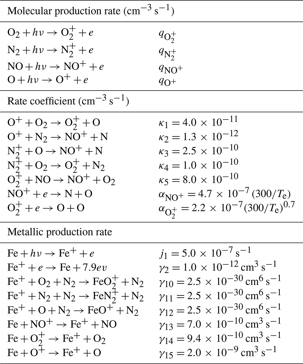
The chemical reactions and respective rate coefficients for production and loss used in MIRE are shown in Table 1. These coefficients were obtained in Chen and Harris (1971) for the molecular ions and in Carter and Forbes (1999) for the metal ions. The coefficients for Mg⁺ are half that of Fe⁺. For detailed information about these equations and coefficients, see Carrasco et al. (2007) and Resende et al. (2017a, b).

Table 1 Chemical reactions for the molecular and metallic constituents used in MIRE.

Therefore, the electronic density profile is given by the sum of the molecular and metal ions, as shown in Eq. (7). The simulations are obtained in a space-time of approximately 0.2 km height every 2 min between 00:00–24:00 UT for altitudes between 86 and 140 km, assuming photochemical equilibrium of the species as initial conditions for the numerical equations to be solved until ion convergence is reached (Carrasco et al., 2007; Resende et al., 2016, 2017a, b; Conceição-Santos et al., 2019; 2020).

$$\begin{array}{}\text{(7)}& n_e=\left[{\mathrm{O}}_{\mathrm{2}}^{+}\right]+\left[{\mathrm{NO}}^{+}\right]+\left[{\mathrm{O}}^{+}\right]+\left[{\mathrm{N}}_{\mathrm{2}}^{+}\right]+\left[{\mathrm{Fe}}^{+}\right]+\left[{\mathrm{Mg}}^{+}\right]\end{array}$$

For the transport term in the continuity equation, MIRE uses the equation of motion that depends on the meridional (U_x) and zonal (U_y) wind components and the electric field $\left(E_{x,y,z}\right)$, as given in Eq. (8).

$$\begin{array}{}\text{(8)}& \begin{array}{rl}{V}_{\mathrm{i}z}& ={\displaystyle \frac{{\mathit{\omega }}_{\mathrm{i}}^{\mathrm{2}}}{\left({\mathit{\nu }}_{\mathrm{in}}^{\mathrm{2}}+{\mathit{\omega }}_{\mathrm{i}}^{\mathrm{2}}\right)}}[\cos I\cdot \sin \cdot U_x+{\displaystyle \frac{{\mathit{\nu }}_{\mathrm{in}}}{{\mathit{\omega }}_{\mathrm{i}}}}\cdot \cos I\cdot U_y\\ & +{\displaystyle \frac{\mathrm{1}}{{\mathit{\nu }}_{\mathrm{in}}}}{\displaystyle \frac{e}{m_{\mathrm{i}}}}\cdot \cos I\cdot \sin I\cdot E_x\\ & +{\displaystyle \frac{e}{{\mathit{\omega }}_{\mathrm{i}}{m}_{\mathrm{i}}}}\cdot \cos I\cdot E_y+{\displaystyle \frac{e}{{\mathit{\nu }}_{\mathrm{in}}{m}_{\mathrm{i}}}}\cdot \left({\displaystyle \frac{{\mathit{\nu }}_{\mathrm{in}}^{\mathrm{2}}}{{\mathit{\omega }}_{\mathrm{i}}^{\mathrm{2}}}}+{\sin }^{\mathrm{2}}I\right)\cdot E_z],\end{array}\end{array}$$

where ω_i is the ion's gyrofrequency, ν_in is the ion-neutral collision frequency, I is the magnetic inclination angle, m_i is the ion's mass, and e is the ion's electric charge. The coordinate system is composed of the x axis pointing south, the y axis pointing east, and the z axis pointing up.

In this work, the wind data used in MIRE were obtained by the SkiYMET meteor radar installed in the OLAP (Observatório de Luminescência Atmosférica da Paraíba) observatory at São João do Cariri (7.23^∘ S, 36.32^∘ W; dip lat. −12.21). The SkiYMET radar monitors the meteor echoes for altitudes ranging from 80 to 100 km (Hocking, 2004; Buriti et al., 2008; Andrioli et al., 2009). However, the height range of interest in this study at MIRE is between 86 and 140 km (Resende et al., 2017a, b). Thus, meridional and zonal wind data observed on meteoric radars were extrapolated with a Lorentz curve fitting for heights from 100 to 140 km. The Lorentz curve was used here for wind amplitude, considering the theory about wind behavior (Lindzen and Chapman, 1969; Forbes and Garrett, 1979), and given according to Eq. (9):

$$\begin{array}{}\text{(9)}& \begin{array}{rl}{U}_{(x\mathrm{0},y\mathrm{0})}^{(\mathrm{24},\mathrm{12},\mathrm{8})}\left(z\right)& ={\mathit{\mu }}_{(x\mathrm{0},y\mathrm{0})}\\ & +{\displaystyle \frac{\mathrm{2}.A_{(x\mathrm{0},y\mathrm{0})}}{\mathit{\pi }}}{\displaystyle \frac{{\mathit{\phi }}_{(x,y)}}{\mathrm{4}.{\left(z-h_{(x\mathrm{0},y\mathrm{0})}\right)}^{\mathrm{2}}+{\mathit{\phi }}_{(x,y)}^{\mathrm{2}}}},\end{array}\end{array}$$

where μ_(x0,y0), A_(x0,y0), φ_(x,y), and h_(x0,y0) are the fitted parameters for the meridional and zonal components of the diurnal (24 h), semidiurnal (12 h), and terdiurnal (8 h) tides. Additionally, the wind phases were obtained by a linear fitting of the observational data. The vertical wavelengths (λ_x,y) can be used from the respective wave phase equations by multiplying the linear coefficient of the fitted curves by the corresponding tidal period, e.g., 24 h for diurnal tide, 12 h for the semidiurnal tide, and 8 for the terdiurnal tide (Buriti et al., 2008). It is important to mention here that we used the extended version of MIRE proposed by Conceição-Santos et al. (2019) with a modification in the λ_x,y of the extrapolated winds, keeping them constant between 100 and 120 km and tending to infinity between 120 and 140 km. Then they were inserted into the MIRE model to show the E_s layer density profiles for the months of December (summer), April (autumn), July (winter), and October (spring) as representative of the seasons. Finally, the wind profiles agreed with the previous study performed with the Wind Image Interferometer (WINDII) aboard the Upper Atmosphere Research Satellite (UARS) between 90 and 270 km seen in Lieberman et al. (2013). Equations (10) and (11) represent, respectively, the meridional and zonal wind components, given by

$$\begin{array}{}\text{(10)}& {\displaystyle }{U}_x\left(z\right)=U_{x\mathrm{0}}\left(z\right)\cos \left({\displaystyle \frac{\mathrm{2}\mathit{\pi }}{{\mathit{\lambda }}_x}}\left(z-z_{\mathrm{0}}\right)+{\displaystyle \frac{\mathrm{2}\mathit{\pi }}{T}}\left(t-t_{x\mathrm{0}}\left(z\right)\right)\right),\text{(11)}& {\displaystyle }{U}_y\left(z\right)=-U_{y\mathrm{0}}\left(z\right)\sin \left({\displaystyle \frac{\mathrm{2}\mathit{\pi }}{{\mathit{\lambda }}_y}}\left(z-z_{\mathrm{0}}\right)+{\displaystyle \frac{\mathrm{2}\mathit{\pi }}{T}}\left(t-t_{y\mathrm{0}}\left(z\right)\right)\right),\end{array}$$

where U_x0(z) and U_y0(z) are the wind amplitudes at height z; λ_x and λ_y are the wavelengths for the respective meridional and zonal components of the diurnal, semidiurnal, and terdiurnal tides; z₀ is a reference height (100 km); and t_x0(z) and t_y0(z) are the wave phases; and T is the tidal period, which can be diurnal (24 h), semidiurnal (12 h), or terdiurnal (8 h).

It is important to mention that this work is the first study in which the terdiurnal tide was implemented in the MIRE model by using the SkiYMET wind profiles obtained from data collected at São João do Cariri. These data were used as representative of the winds over the observatory of Palmas since no other measurements at any closer station were available simultaneously with the ionosonde observations. Thus, the inferred neutral winds and atmospheric tides were included in Eqs. (10)–(11) of MIRE to simulate the E_s layer dynamics over Palmas. A more detailed description about the radar system and the methodology used to compute the neutral wind parameters is available in Resende et al. (2017a).

3 Results and discussion

3.1 Terdiurnal tide periodicities in E_s layer occurrences

Figure 1a shows the temporal variation (in UT) of the percentage occurrence of the “h”, “c”, and “f/l” types of E_s layers during the summer solstice months of 2008/2009. The occurrences of the “f” and “l” types were grouped into one since both have nearly the same ionogram profile; however, the “l” type manifests only during the daytime, and the “f” type is typically nocturnal (Conceição-Santos et al., 2020). From December 2008 to February 2009 (summer), a total of 48 d of data was recorded by the ionosonde of Palmas, which corresponds to 2859 ionograms. The daytime occurrence of E_s layers was 65.58 % (156.25 h), while 34.42 % (82 h) occurred during nighttime. The $E_{{\mathrm{s}}_{\mathrm{f}/\mathrm{l}}}$ types were the most frequent, with an overall rate of 72.61 % (173 h).

Notice that a slight increase of the E_s layer occurrence is observed between about 01:00–02:00 UT (LT = UT−3 h) with ∼ 17 % rate, and the $E_{{\mathrm{s}}_{\mathrm{f}/\mathrm{l}}}$ layers are predominant during nighttime. Then a drop occurs near dawn at 08:00 UT, reaching occurrence rates of less than ∼ 7 %. Approximately 8 h after the first increase, the E_s layers' percentage of occurrence enhances markedly, reaching ∼ 50 % at 11:00 UT. This peak at 11:00 UT coincides with the increase in the occurrence rates of the “c” and “h” types of E_s layers. The $E_{{\mathrm{s}}_{\mathrm{c}}}$ and $E_{{\mathrm{s}}_{\mathrm{h}}}$ layers are formed starting at dawn, after 10:00 UT, and cease at dusk around 20:00 UT. The $E_{{\mathrm{s}}_{\mathrm{c}}}$ type corresponds to 13.47 % (total of 32.08 h), while the $E_{{\mathrm{s}}_{\mathrm{h}}}$ type corresponds to a rate of 13.92 % (total of 33.17 h). It is clearly noticed that the $E_{{\mathrm{s}}_{\mathrm{h}}}$ layer predominates over the other E_s types between around 11:00–12:00 UT (∼ 25 % and ∼ 23 %, respectively). After this peak in the occurrence rate of the E_s types, the percentage of occurrence starts to decrease again, reaching a value of ∼ 7 % between 15:00 and 16:00 UT. However, after 17:00 UT, the occurrence rate starts to increase again and attains values of ∼ 41 % between around 19:00–21:00 UT. The three increases observed in the plot of occurrence rates of E_s layer types with 8 h periodicities suggest a modulation associated with the terdiurnal tide during the summer period.

The analysis of the temporal occurrence of E_s layer types over Palmas was extended for the autumn, winter, and spring seasons, as seen in Fig. 1. In this figure, we show the occurrence rates for autumn (panel b), winter (panel c), and spring (panel d). As noted earlier for the summer, the $E_{{\mathrm{s}}_{\mathrm{f}/\mathrm{l}}}$ types were also predominant during nighttime, and the $E_{{\mathrm{s}}_{\mathrm{c}}}$ and $E_{{\mathrm{s}}_{\mathrm{h}}}$ types occurred only during daytime. At 12:00 UT in winter and between 11:00–15:00 UT in spring, the $E_{{\mathrm{s}}_{\mathrm{f}/\mathrm{l}}}$ layers were not predominant. In the autumn months, we observed three well-defined maxima in the occurrence rate of E_s layer types, whereas in the winter (∼ 9 % at 02:00 UT) and spring (∼ 5 % at 02:00 UT) months the first peak is not well defined. However, we observed clear second and third ones at around 10:00–12:00 and 19:00–20:00 UT, respectively, indicating the possible influence of the terdiurnal tide. The slight increase in the occurrence rate between around 03:00–04:00 UT during the spring season might suggest that, besides the dominant terdiurnal tidal periodicities, there was also a weaker quarter-diurnal (6 h) oscillation affecting the E_s layer development. By comparing the results shown in Fig. 1, it is clearly noticed that another peak of ∼ 47 % was observed between around 10:00–11:00 UT during the spring season. Furthermore, the larger amplitudes of the E_s layer occurrence rates associated with the terdiurnal tide modulation were observed during the summer and spring months.

The E_s layers in Fig. 1 ($E_{{\mathrm{s}}_{\mathrm{f}/\mathrm{l}}}$, $E_{{\mathrm{s}}_{\mathrm{c}}}$, and $E_{{\mathrm{s}}_{\mathrm{h}}})$ are formed by the wind shear mechanism due to the tidal wind component in the Southern Hemisphere (Arras et al., 2009; Haldoupis, 2012; Pancheva et al., 2013; Fytterer et al., 2014; Yu et al., 2019). The $E_{{\mathrm{s}}_{\mathrm{h}}}$ type forms and disappears very fast compared to the $E_{{\mathrm{s}}_{\mathrm{f}/\mathrm{l}}}$ and $E_{{\mathrm{s}}_{\mathrm{c}}}$ types, which indicates that this type of $E_{{\mathrm{s}}_{\mathrm{h}}}$ layer may be formed mostly by molecular ions that have shorter lifetimes than metal ions (Plane, 2003; Plane et al., 2015). Also, it is possible to observe in Fig. 1 that the $E_{{\mathrm{s}}_{\mathrm{h}}}$ type shows a higher percentage in the peak rates between 11:00 and 12:00 UT, with a higher percentage occurring in summer. Oikonomou et al. (2014) explained that the meridional wind component is dominant over the zonal wind component above ∼ 130 km in the formation of high E_s layers. On the other hand, Conceição-Santos et al. (2020) analyzed the $E_{{\mathrm{s}}_{\mathrm{h}}}$ type, and they concluded that the predominant wind direction controlling their formation and dynamics had equal importance for both the zonal and meridional components. Generally, the $E_{{\mathrm{s}}_{\mathrm{h}}}$ layer performed a downward movement due to the wind dynamics, reaching heights of around 100 km and then becoming the $E_{{\mathrm{s}}_{\mathrm{c}}}$ or $E_{{\mathrm{s}}_{\mathrm{f}/\mathrm{l}}}$ layers. Haldoupis et al. (2006) mentioned that vertical shear in the zonal and meridional winds work together to generate the descent of the $E_{{\mathrm{s}}_{\mathrm{h}}}$ layers. In fact, the E_s layer types shown in Fig. 1 strongly suggest that the formation mechanism of the E_s layers is the wind shear, emphasizing the main mechanism of the E_s layer development at low latitudes.

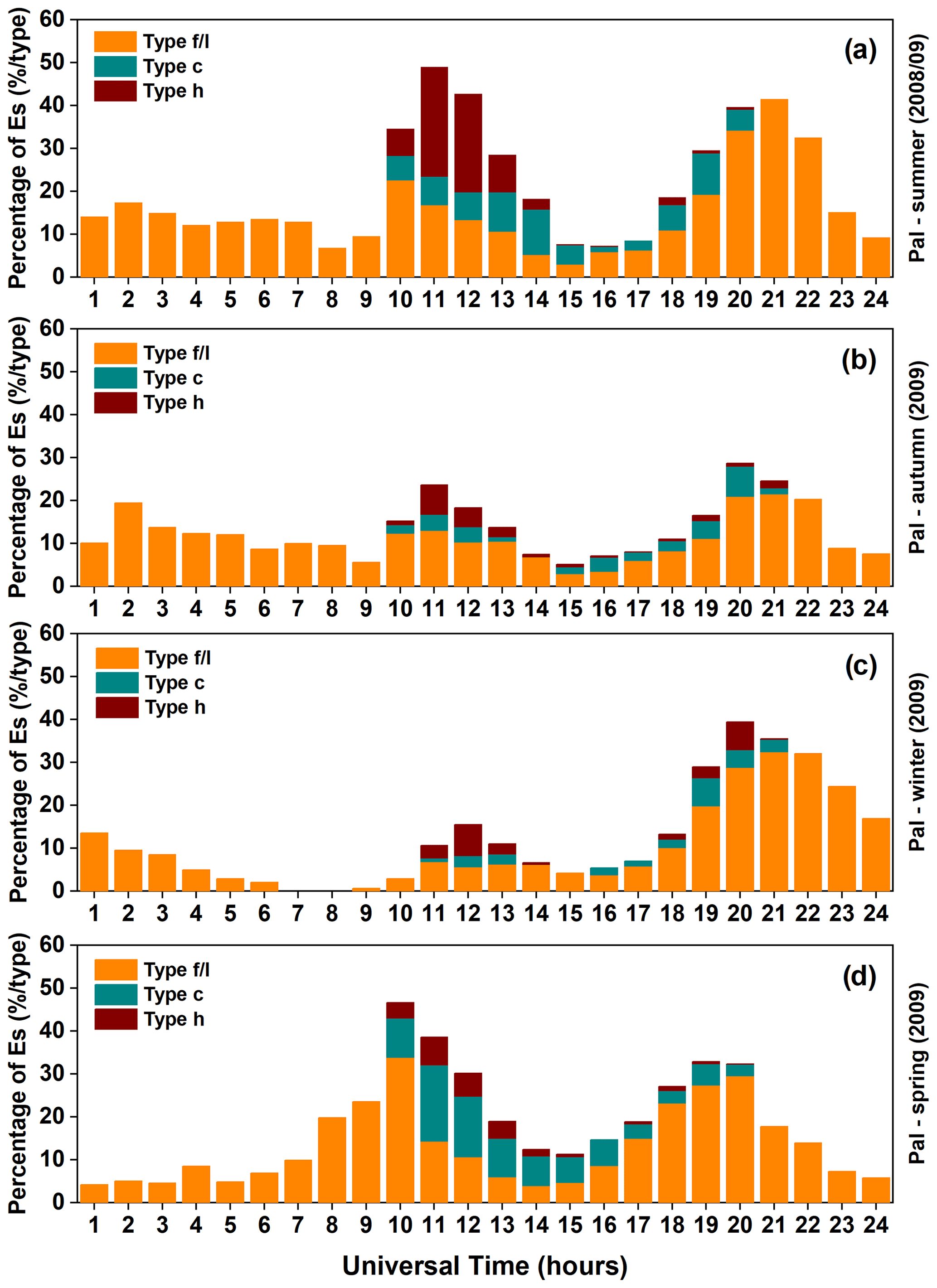
Figure 1 Temporal variation of the E_s layer occurrence rates divided into different types over Palmas during the summer (a) autumn (b), winter (c), and spring (d) months of the year 2008/2009.

Figure 2 depicts the temporal variation of the E_s layer (h^′E_s) for the “h”, “c”, and “f/l” types during the four seasonal periods at Palmas. It is seen from Fig. 2 that the $E_{{\mathrm{s}}_{\mathrm{h}}}$ layers were formed at higher altitudes between around 130 and 150 km, whereas the $E_{{\mathrm{s}}_{\mathrm{c}}}$ layers were observed at altitudes ranging from 110 to 130 km. As expected, the $E_{{\mathrm{s}}_{\mathrm{c}}}$ and $E_{{\mathrm{s}}_{\mathrm{f}/\mathrm{l}}}$ layers were mostly observed at altitudes below 110 km, although during some specific hours at all seasons they attained heights of ∼ 130 km. The $E_{{\mathrm{s}}_{\mathrm{h}}}$ layer tends to move down to lower heights in the E region, changing into types “c” or “l” when they reach 100 km (Conceição-Santos et al., 2020). Another relevant aspect to be observed in Fig. 2 is related to the distribution of h^′E_s during the times of maximum occurrence rate of the E_s layer types, which is possibly associated with the terdiurnal tide. During the peaks in the frequency of occurrence of E_s layers at around 10:00–12:00 and 18:00–20:00 UT, Fig. 2 reveals for all seasons that the E_s layers attained their highest altitudes. Otherwise, during the time of the first increment at around 01:00–02:00 UT, significant changes in the heights of the $E_{{\mathrm{s}}_{\mathrm{f}/\mathrm{l}}}$ layers were not evident. However, it seems that the terdiurnal tidal oscillations had some role in the formation of the $E_{{\mathrm{s}}_{\mathrm{h}}}$ layers during the daytime.

As is already known, tides are the major sources of vertical wind shear (Arras et al., 2009; Haldoupis, 2012; Pancheva et al., 2013; Fytterer et al., 2014; Yu et al., 2019; Jacobi and Arras, 2019). Thus, tide-like structures are expected to influence the occurrence rates of E_s layers strongly. As noticed in Fig. 2, most of the E_s layers are concentrated at heights below 120 km. According to Fytterer et al. (2014), the influence of the terdiurnal oscillations on E_s formation and evolution is restricted to heights between around 100–120 km. Thus, in this height range, the terdiurnal tidal oscillations may have a similar amplitude to the diurnal and semidiurnal tides (Zhao et al., 2005; Venkateswara Rao et al., 2011; Moudden and Forbes, 2013; Fytterer et al., 2014), and they can also play an important role in modulating the E_s layers. Bergsson and Syndergaard (2022) used the parameter h^′E_s to investigate the relationship of the E_s layers at mid- and low-latitude regions with solar activity. They showed that h^′E_s values vary with the seasons and significantly depend on solar activity in the nighttime period. Haldoupis et al. (2006) applied the height–time–intensity (HTI) method to analyze the descent of the E_s layers. The authors observed the formation of an E_s layer at ∼ 120–130 km that descends to ∼ 100 km at dusk. Also, they observed that the formation of E_s layers at heights above 125 km during nighttime has a higher descent rate than the daytime ones. Haldoupis (2011) and Andoh et al. (2020) mentioned that the zonal and meridional wind is equally efficient at ∼ 125 km altitude where ν_i∼ω_i. On the other hand, at lower (higher) altitudes, the zonal (meridional) wind component becomes predominant in ion convergence by wind shear. This behavior occurs because at higher heights ν_i≪ω_i, making the ions more magnetized, decreasing the efficiency of the zonal component, and increasing the contribution of the meridional component. Thus, the $E_{{\mathrm{s}}_{\mathrm{h}}}$ layers in Fig. 2 may indicate a predominance of meridional wind action, because these layers generally form at altitudes above 125 km and disappear quickly. The E_s layer heights in summer shown in Fig. 2 are in good agreement with the analyses by Yu et al. (2019) for both hemispheres using RO, where they observed a seasonal variation in the altitude–latitude distribution of the E_s layer intensity with the highest values at 125 km in the Southern Hemisphere summer and a wider latitudinal extent between 10 and 75^∘ S. Other work, such as Haldoupis and Pancheva (2006), used the h^′E_s parameter to analyze the terdiurnal tidal oscillations over the E_s layers. They concluded that the 8 h oscillation is more pronounced in h^′E_s than in the frequencies (foE_s) and contributes to decreasing the E_s layers with time.

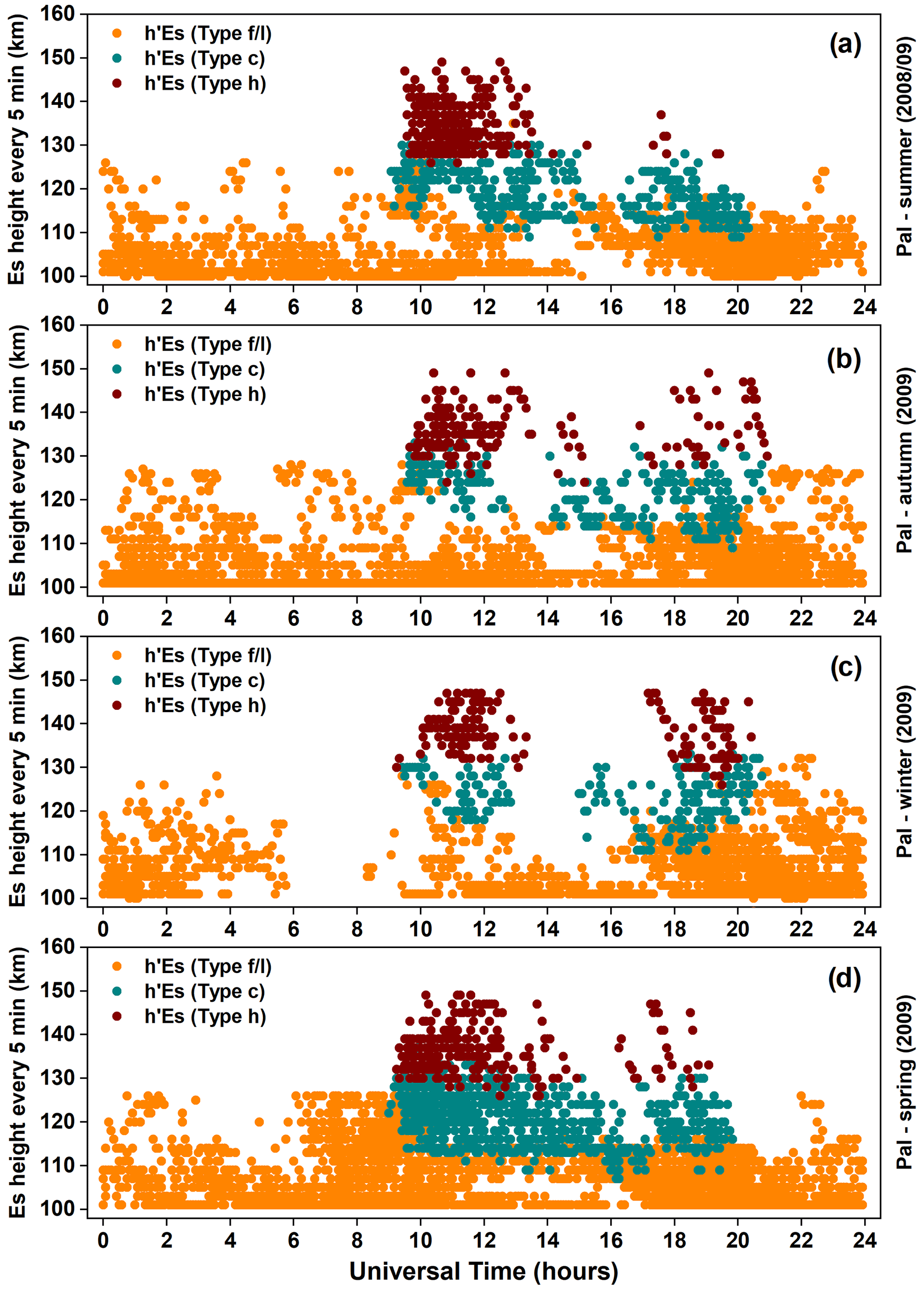
Figure 2 Virtual height distribution of the E_s layer types as a function of time (in UT) over Palmas during summer (a), autumn (b), winter (c), and spring (d).

All types of E_s layers were grouped to calculate the temporal variation of the total percentage (black line) of occurrence of the E_s layers observed in Palmas during the four seasons. These results of total occurrence are shown in Fig. 3. The three maximum values in the total occurrence rate of the E_s layers during the summer and autumn months agree with the results observed before in Fig. 1a and b. As already seen, these peaks are approximately 8 h apart from each other, revealing a possible modulation by the terdiurnal tide. Analogously to what was observed in Fig. 1c, during winter, only two maxima in the total percentage of occurrence are noticed, one being at around 11:00–12:00 UT and another at about 19:00–20:00 UT. As for the spring, a maximum in the occurrence rate was observed during the morning between approximately 09:00–10:00 UT, and ∼ 8 h later another maximum was observed at dusk between around 18:00–20:00 UT. However, a small increase of ∼ 8.5 % was observed in the total percentage rate between around 03:00–04:00 UT during the spring, which reveals again the possible effect of a weaker 6 h tidal mode embedded in the temporal occurrence rate of the E_s layers.

Figure 3 Temporal variation of the E_s layer occurrence over Palmas separated into individual months during the summer (a), autumn (b), winter (c), and spring (d).

Figure 3 shows the monthly percentage of occurrences of E_s layers divided by seasons. In summer (Fig. 3a), the terdiurnal modulation is dominant during February 2009. On the other hand, in December 2008 and January 2009, a first increase in the occurrence rate observed previously at around 01:00–02:00 UT is practically absent. This is probably related to the tendency for the amplitude of the migrating terdiurnal tide with zonal wavenumber 3 (TW3) to increase, generally from January to March within ± 10^∘ of latitude (Moudden and Forbes, 2013; Pancheva et al., 2013). Thus, the maximum peaks in the occurrence rates observed in February of 2009 are higher than those observed in December/January, owing to the fact that this time is when the summer solstice starts in the Southern Hemisphere. This result also agrees with Guharay et al. (2013), where a smaller terdiurnal tidal range for the December/January months and an increase of this component in February at low-latitude stations over the Brazilian sector are shown.

During autumn (Fig. 3b), the 8 h tidal oscillations are noticed in the results of April and May. Notice that the three peaks in the occurrence rates in April are higher than in the other months. Unlike the results shown in Fig. 1, Fig. 3c reveals a weaker increase in the percentage of occurrence (∼ 12 %) between around 01:00–03:00 UT, a clear second peak after 8 h, and a strong peak at approximately 19:00–21:00 UT. The total percentage of occurrence (Fig. 3, black line) between 01:00–05:00 UT during winter was strongly influenced by the occurrence rate observed in August. Guharay et al. (2013) also found a significant increase in tidal amplitude in the autumn and minimum values for winter and early summer. Finally, in spring, the modulations associated with the terdiurnal tide are marked during September, October, and November.

The temporal variation of the total percentage of occurrence of E_s layers was plotted in intervals of 20 min, as shown in Fig. 4. The results for summer (red), autumn (purple), winter (blue), and spring (green) are shown as line plots. Then a nonlinear polynomial regression was applied to fit the occurrence rate curves for each season (black lines). The shadowed bands in the fitted curves denote the 95 % confidence interval of the best-fitted parameters. It is possible to note that the curves of percentage rates are mostly within the 95 % confidence range of the nonlinear curves. However, when the peaks in the occurrence rates are above the 95 % level of confidence, the most significant effect of the terdiurnal tide on the formation and dynamics of E_s layers is revealed.

It is worth noting in Fig. 4 the 8 h periodicities in the fitted curves of all the seasonal periods. During winter, the first increase in the occurrence percentage at around 02:00–03:00 UT is not as pronounced as in the other seasons, but now it is more perceivable than Figs. 1 and 2 and also depicts the pattern seen in Fig. 3 for June and July. According to Du and Ward (2010), the maximum amplitudes of the terdiurnal tide are confined between ± 50^∘ of latitude and tend to occur in winter between 80 and 100 km of altitude. As the E_s layers over Palmas were observed above 100 km, this may partly explain why the terdiurnal oscillations were less pronounced in winter.

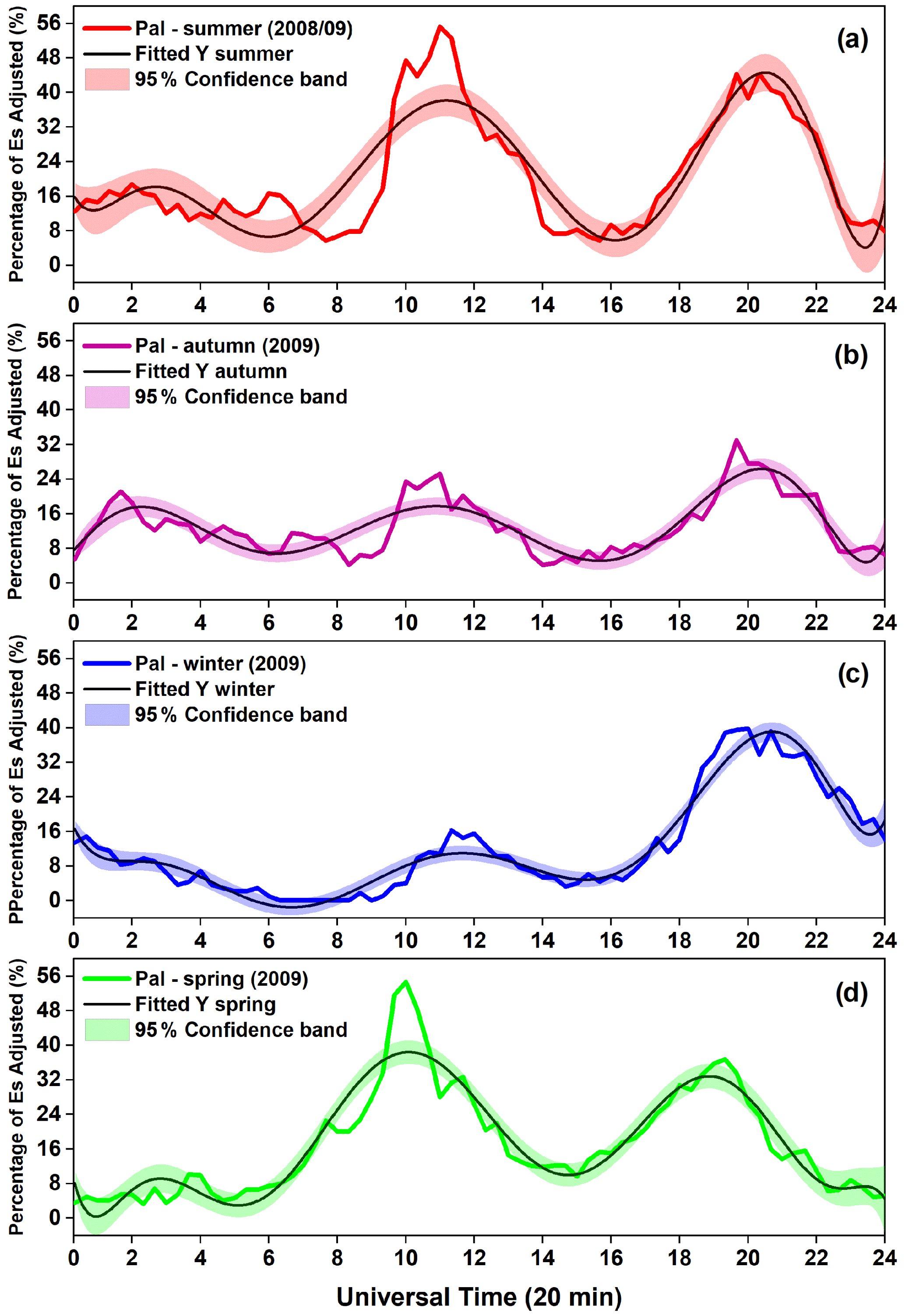
Figure 4 Temporal variation of E_s layer occurrences obtained in intervals of 20 min during summer (red line, a), autumn (purple line, b), winter (blue line, c) and spring (green line, d) seasons. The black lines in the panels are the fitted curves of the occurrence rates by applying a nonlinear regression. The shadowed bands in the fitted curves denote the 95 % confidence interval of the best-fitted parameters.

The results in Fig. 4 also agree with the study of Moudden and Forbes (2013), who analyzed 10 years of data and highlighted that the migrating terdiurnal tide reaches higher amplitudes near the magnetic equator at altitudes above 100 km but with higher amplitudes for the Southern Hemisphere. Pancheva et al. (2013) also analyzed 8 years (2002–2009) of terdiurnal tidal (TW3) oscillations and found that between latitudes of ± 10^∘, the amplitude of the terdiurnal tide at an altitude of ∼ 90 km had a maximum in the month of February, and that at 110 km altitude at low latitudes (± 30^∘) it had a maximum amplitude during the summer and winter.

The 3D color map surfaces in Fig. 5 present the top frequencies of layer E_s (ftE_s) distributed per day (in UT) for the summer, autumn, winter, and spring seasons. The color assigned in the graphs is related to the E_s layer intensity. It is important to mention here that there were problems with the ionosonde equipment during the summer and the winter at Palmas. Therefore, there are some gaps in the data with values corresponding to zero on the scale of values of the ftE_s but not causing interference in the previous results presented here.

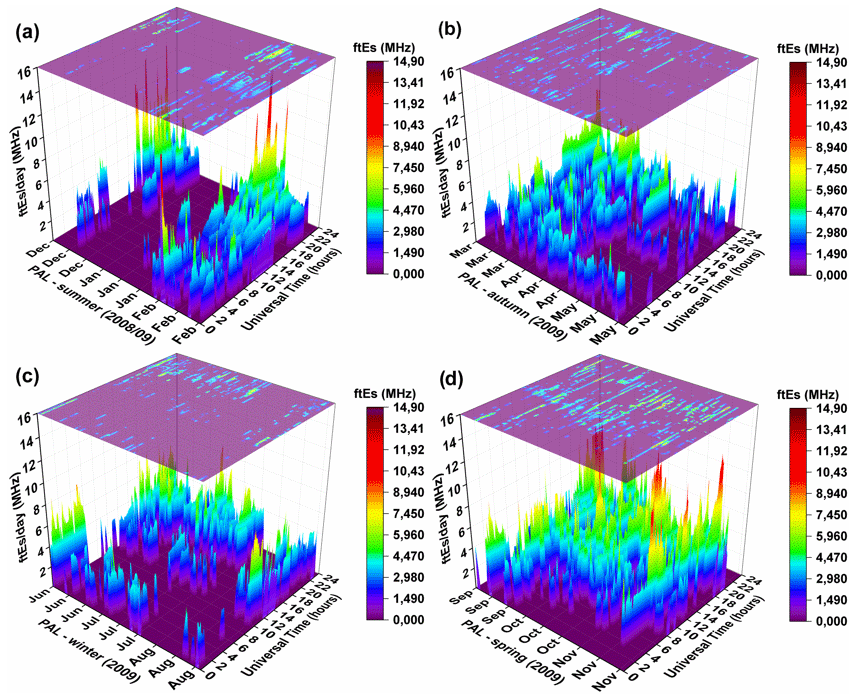
Figure 5 The 3D color map surfaces of the E_s layer top frequency (ftE_s) distributed per day (in UT) for the summer (a), autumn (b), winter (c), and spring (d) over Palmas.

Figure 5 reveals that in autumn and winter the ftE_s magnitudes were lower than those observed during the summer or spring months. Such ftE_s values are almost always below 10 MHz. On the other hand, it was observed that ftE_s values were above 10 MHz during spring. Summer presented the highest ftE_s values in the late afternoon, whose maximum intensity was 14.9 MHz (20:00 UT). This maximum intensity of the ftE_s was detected in early February (2 June 2009) and some days in December 2008. We believe that the high values of ftE_s observed here in early February may be due to the event of sudden stratospheric warming (SSW) that occurred between late January and early February of 2009 (Wang et al., 2011; Fuller-Rowell et al., 2011). This SSW event had global effects on the semidiurnal (SW2) and terdiurnal (TW3) tidal amplitudes, as well as planetary waves (PW1 and PW2) (Wang et al., 2011; Fuller-Rowell et al., 2011; Lin et al., 2012; Jin et al., 2012). It is well known that during a SSW the planetary waves can propagate vertically into the lower thermosphere and interact with the tides that dominate the dynamics in the ionospheric region. Thus, they can influence the development of the E_s layers formed at this altitude (Liu and Roble, 2002; Lin et al., 2012; Fytterer et al., 2014). Wang et al. (2011) showed an SW2 tidal growth peaking after the SSW maximum and a TW3 decrease in the Southern Hemisphere. Subsequently, between 100–120 km altitude at 20–60^∘ S, the rapid growth of tidal amplitude TW3 and a considerable decrease of SW2 occurred. The authors attributed this to a transfer of energy from the SW2 to the TW3 tide in both hemispheres. Jin et al. (2012) showed that a notable increase in TW3 amplitude occurred at 115 km altitude after the SSW at low latitudes between 0–30^∘ S. Therefore, the prominent peak in ftE_s (Fig. 5a) may indicate further evidence of the influence of the terdiurnal tide on the development of the E_s layer. The results in Fig. 5 are in good agreement with the Yu et al. (2022) analysis. Those authors compared the observational data using RO with a modeling of the E_s layers concerning the seasons. The authors show that summer and spring have more-intense E_s layer occurrences than autumn and winter in the Northern Hemisphere and Southern Hemisphere. Additionally, the results in Fig. 5 are consistent with Tang et al. (2022), showing that the TW3 modulates the E_s layers between 100–110 km of latitudes ± 10^∘.

A power spectrum analysis with periodograms was performed using the fbE_s data (Fig. 6) to demonstrate that the periodicities present in the observational data are associated with tidal effects. The peak of the diurnal tide has been suppressed in Fig. 6 for better visualization of the terdiurnal tide. The 6 h peak associated with a quarter-diurnal tide can be observed during the autumn, winter, and spring seasons.

Xu et al. (2014) showed that the nonlinear interaction between the planetary wave and the quarter-diurnal tide might be the source of the formation of the terdiurnal tides, and the nonlinear interaction between the diurnal tide and the terdiurnal tide may be the primary source of the quarter-diurnal tide. This may account for the increase/decrease in the 8 and 6 h peaks observed in the periodogram analyses of the seasons in Fig. 6. Guharay et al. (2013) also noted the presence of the quarter-diurnal tide at the latitude of São João do Cariri, which is a region of the Brazilian sector near Palmas, but indicated an adequate analysis would be needed to confirm this 6 h oscillation. Lima et al. (2012) showed that the quasi-two-day wave (QTDW) and other periodicities are also present in the São João do Cariri region. Thus, it is possible that the occurrence of the 8 and 6 h oscillations shown in Fig. 6 occurred by the nonlinear interaction between the planetary waves and the terdiurnal and quarter-diurnal tides, in addition to the nonlinear interactions between the diurnal and semidiurnal tides (Manson et al., 1982; Teitelbaum and Vial, 1991; Pancheva, 2000; Chang et al., 2011, 2013; Gu et al., 2017). This topic is beyond the scope of this work due to the lack of wind data, but it can be explored in the future.

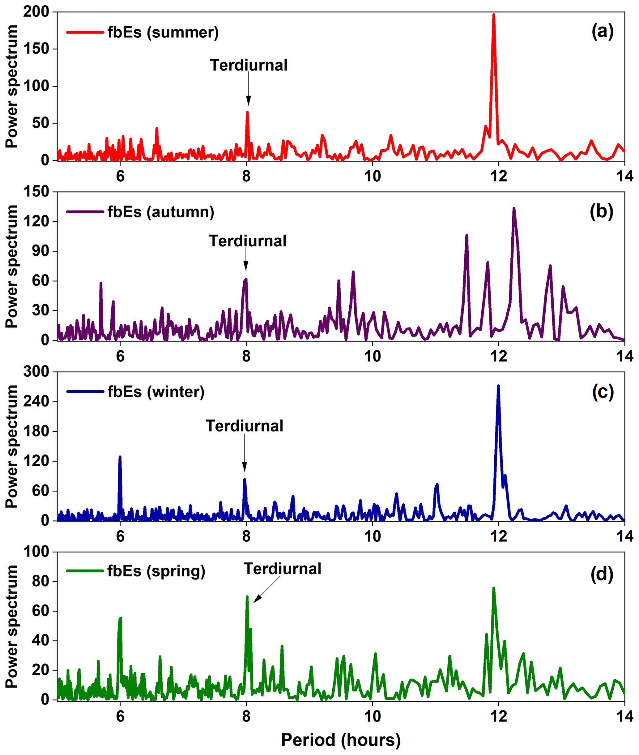
Figure 6 Periodogram analysis of the fbE_s with the power spectrum representations of (a) summer, (b) autumn, (c) winter, and (d) spring. The best-fitting peaks correspond to the 99 % confidence interval of the fbEs parameters.

Lastly, the results of the E_s layer intensity do not provide a conclusion that terdiurnal tide is influencing the densities, as is shown in height. However, we found some correlation between the strong E_s layer and the most terdiurnal modulation, as seen during the summer. Thus, we used a model to analyze the terdiurnal tide role in the E_s layer behavior that will be presented in the following section.

3.2 E region simulations

The simulations of the ionospheric electron density profiles (in logarithmic scale) between 86 and 140 km concerning universal time are shown in Fig. 7. We considered in the simulations the three tidal structures (semidiurnal, diurnal, and terdiurnal periodicities) for the zonal and meridional wind components. The panels on the left column of Fig. 7 refer to the results of diurnal and semidiurnal tides (D + S), while the panels on the right column show the simulation results considering the diurnal, semidiurnal, and terdiurnal tides (D + S + T). We selected data from different months to represent each seasonal period: December 2008 (summer, panel a), April 2009 (autumn, panel b), July 2009 (winter, panel c), and October 2009 (spring, panel d). These months were chosen because, during the period analyzed here, they presented better diurnal, semidiurnal, and terdiurnal wind data estimations from meteor radar observations at São João do Cariri, and there is already a study on the terdiurnal tide with data from this station in the Brazilian sector that can be found in Guharay et al. (2013). As we mentioned before, these wind data were used as input to the MIRE model. The thin traces of enhanced electron density seen in the plots of density profiles in Fig. 7 denote the presence of the E_s layers.

In the plots of electron density profile shown in Fig. 7a for December (summer), it is possible to see that when only diurnal and semidiurnal tides (D + S) are considered in the simulations, the E_s layer is formed at 16:00 UT just below 130 km altitude. This E_s layer tends to move downward throughout the night and reaches an altitude of ∼ 115 km near dawn at 09:00 UT. During the day, it continues to descend slowly until reaching ∼ 110 km at around 16:00 UT. The density of this E_s layer has a maximum value of ∼ 10^5.1 electrons cm⁻³. When adding the terdiurnal tide (D + S + T) in the simulations, the results in the right panel of Fig. 7a clearly reveal that the layer is formed at higher altitudes above 135 km at around 14:00 UT. Analogously to what was observed from the D + S simulation, the E_s layer descended continuously and reached ∼ 110 km 24 h later. Also noted is an intensification of the maximum E_s layer density to ∼ 10^5.8 electrons cm⁻³.

The results of the MIRE simulations for April (autumn) are presented in Fig. 7b. The D + S simulation shows a thick E_s layer starting at around heights of more than 138 km and descending continuously, reaching ∼ 120 km altitude at 24:00 UT. The maximum density of this E_s layer is about ∼ 10^5.0 electrons cm⁻³. By adding the terdiurnal tide (D + S + T) into the simulation, the results show that the most intense E_s layer forms at about ∼ 140 km altitude at 03:00 UT and moves downward. Notice that along almost its entire descent trajectory the layer density is notably larger (∼ 10^5.2 electrons cm⁻³) compared to the D + S simulation.

The panels in Fig. 7c for July (winter) show similar results from the D + S and the D + S + T simulations regarding the height of formation and descent of the E_s layers. In both simulations, the E_s layer is formed at around 06:00 UT at heights of ∼ 140 km. As the layer descends throughout the day, the electron density increases to ∼ 10^4.5 electrons cm⁻³ for the D + S simulation and to ∼ 10^5.0 electrons cm⁻³ for the D + S + T simulation. From 22:00 UT until around 04:00 UT, the layer stops descending and becomes thicker, and its electron density decreases to ∼ 10^4.0 electrons cm⁻³. Furthermore, it presents a slight rise from ∼ 117 to 122 km. Then the E_s layer starts to descend again until pre-sunrise hours.

Figure 7 Density profiles of the E_s layers simulated by MIRE during (a) December (summer), (b) April (autumn), (c) July (winter), and (d) October (spring).

Table 2 Comparison of the simulated E_s layer densities in MIRE with the D + S, D + S + T component and the maximum average daily density from the observed ionosonde data.

Finally, the MIRE simulations for the month of October (spring) present in Fig. 7d a very distinct diurnal behavior between the D + S and D + S + T simulations. The E_s layer in the simulation due to D + S is formed during daytime at ∼ 140 km. This layer moves downward, reaching ∼ 125 km at 24:00 UT. The results show that this layer continues to move downwards throughout the night and remains until around 12:00 UT when it attains ∼ 107 km. A marked feature observed along the descent course of this layer is the presence of oscillations in its height. The maximum electron density was ∼ 10^4.9 electrons cm⁻³ and reached ∼ 10^5.3 electrons cm⁻³ with the D + S + T component. Such oscillations seen in the traces of E_s layers for both plots of Fig. 7d have already been reported by Conceição-Santos et al. (2020) as possible interactions between gravity/planetary waves and tides.

Additionally, according to Lilienthal et al. (2018), the terdiurnal tide can only occur if both the diurnal and the semidiurnal tides show considerable amplitudes. This is consistent with our results since the terdiurnal tide alone was not able to generate E_s layers in the simulations (not shown here). Moudden and Forbes (2013) compared diurnal, semidiurnal, and terdiurnal tides, and they stated that there is a strong possibility that the non-linear interaction between diurnal and semidiurnal tides is the main source of terdiurnal tide formation. Thus, depending on altitude and latitude, the terdiurnal tide can exhibit amplitudes with significant magnitude, and this can play an important role in the dynamics and modulations of E_s layer densities (Moudden and Forbes, 2013; Pancheva et al., 2013; Fytterer et al., 2013, 2014).

By using radio occultation (RO) data, Fytterer et al. (2014) performed a global analysis of the effect of the terdiurnal tide on the occurrences of the E_s layers. They used data collected in the period from 2006 to 2012 during the four seasonal periods for latitudes of $\pm \mathrm{60}{}^{\circ }$ and altitudes ranging between 85 and 115 km. The authors found two amplitude maxima in the terdiurnal tide signature over the E_s layers during the solstice that maximize between 10 and 40^∘ latitude in both hemispheres. In addition, they also found similar behavior for low-latitude equinox conditions in both hemispheres for altitudes above 100 km. Thus, the intensification of the E_s layer densities obtained here from MIRE simulations is in accordance with the observations in Fytterer et al. (2014). In summer and spring, the simulations showed a more intense E_s layer variation when adding the 8 h tide. This behavior can cause high ftE_s to be observed in such seasons. Finally, our results show that the inclusion of the terdiurnal tide caused an increase in the electron density of the E_s layers for all seasonal periods.

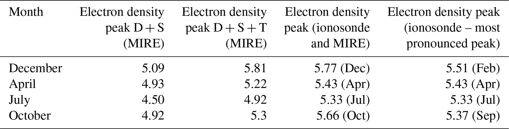
The simulations show that the electron density of the E_s layer increases when we include the terdiurnal tide. To see this behavior better and to compare it with the ionosonde data, we show Table 2. This table contains the results of maximum electron density considering D + S and D + S + T simulations, as well as the maximum average daily electron density observed from the ionosonde data for the same months used in MIRE. Also, we included the maximum electron density of the most pronounced peak in our observational data. We used the ftE_s parameter to calculate the electron density. The density is given in electrons per cubic centimeter on the logarithmic scale.

In general, in Table 2, it is possible to notice that the maximum electron density observed in ionosonde data agreed with the simulations considering the terdiurnal tide component. Notice that there are close values between the densities of the E_s layer simulated in MIRE and the value of the maximum mean daily density observed in the ionosonde data in December. The value of the maximum average daily density observed in February, the month that best represented the 8 h oscillation in Fig. 3, is also in good agreement with the result simulated in MIRE. Also, the months of April and July coincided with the best 8 h oscillation in the percentages of E_s layers in Fig. 3 and simulations for D + S + T. The densities of the E_s layers modeled in MIRE with D + S + T are also in good agreement with the densities of the E_s layers observed with the ftE_s values in Fig. 5, where higher values are shown for summer and spring and lower values for autumn and winter. Finally, October followed the pattern found in December and April, showing good agreement between the simulated E_s layer densities with the terdiurnal tidal component and the maximum mean daily density observed in the ionosonde data. Thus, we notice that the terdiurnal component is important to the E_s layer formation around the months analyzed in this study.

4 Conclusions

This paper presented an analysis of the effect of terdiurnal tidal modulation on the occurrence rate of the E_s layers observed during the years 2008/2009 in Palmas, a low-latitude station located in Brazil. We used ionosonde data and simulations to investigate the effect of terdiurnal (8 h) tidal periodicities on the formation of the E_s layers during different seasonal periods. The main results of this study are summarized as the following:

1. The $E_{{\mathrm{s}}_{\mathrm{f}/\mathrm{l}}}$ is the most common type found in all seasons, while types $E_{{\mathrm{s}}_{\mathrm{c}}}$ and $E_{{\mathrm{s}}_{\mathrm{h}}}$ appear exclusively in the daytime over Palmas, agreeing with the previous results shown in Conceição-Santos et al. (2020). This behavior means that the meridional and zonal tidal wind component is acting for the most time over this station.

2. We observed three peaks in the E_s layer behavior for all seasons, revealing that the terdiurnal tide (8 h) can modulate their formation. This fact is very clear during the summer and spring. In summer, the 8 h modulation is controlled mainly by the E_s layer occurrence in February, probably due to the terdiurnal tide having lower amplitudes in the summer onset. Although autumn shows an 8 h modulation in the E_s layer occurrence, the first peak is not well-defined in March. During the winter, August has a poor rate in the terdiurnal oscillation of the E_s layer occurrence compared to June and July.

   The 8 h modulation in the E_s layer development over Palmas was confirmed using a nonlinear regression for each season. It is worth noting the 8 h periodicities in the fitted curves of the E_s layer rates in all seasonal periods, evidencing a possible effect of the terdiurnal tide on the development of E_s layers. This behavior is less pronounced during the winter, agreeing with the maximum amplitudes of the terdiurnal tide occurring between 80 and 100 km of altitude in this season. Therefore, as the E_s layer appeared above 100 km, we do not have an 8 h periodicity clearly in our data here.

3. The ftE_s had lower values in the autumn and winter than those observed during the summer or spring months (below 10 MHz). Summer presented the highest ftE_s values that can be due to the gradient drift instability of the equatorial electrojet (EEJ) current, which is effective during the magnetic storms in the boundary equatorial magnetic sites, as is the case of the Palmas region. The disturbed electric fields can superimpose the wind shear mechanism during disturbed periods. As in this work, we do not separate the quiet and disturbed days; a more in-depth study of this E_s layer development will be necessary, and we intend to present it in the future. The month of February showed a prominent peak at ∼ 20:00 UT of 14.9 MHz that may be associated with the sudden stratospheric warming (SSW) that occurred in early 2009 and had global influences on atmospheric phenomena.

4. The results of the periodogram analysis using the fbE_s data showed the presence of the terdiurnal tide in all four seasons, indicating that this tidal component contributed to modulate the E_s layer development over Palmas. Besides the expected diurnal and semidiurnal tidal components, we also found in this analysis the 6 h tidal periodicity, which clearly appeared in the power spectrum signatures during autumn, winter, and spring seasons.

5. The results show that the densities of the E_s layers simulated in MIRE are more intense when the terdiurnal tidal component is added to the diurnal and semidiurnal tides, agreeing with the observations previously reported in the work by Fytterer et al. (2014). Comparisons between simulated and observed E_s layer peak electron densities have shown an overall good agreement during the 4 months analyzed here.