Diagnostic study of geomagnetic storm-induced ionospheric changes over very low-frequency signal propagation paths in the mid-latitude D region

We performed a diagnostic study of geomagnetic storm-induced disturbances that are coupled to the mid-latitude D region by quantifying the propagation characteristics of very low-frequency (VLF) radio signals from transmitters located in Cumbria, UK (call sign GQD), and Rhauderfehn, Germany (DHO), and received in southern France (A118). We characterised the diurnal VLF amplitudes from two propagation paths into five metrics, namely the mean amplitude before sunrise (MBSR), the midday amplitude peak (MDP), the mean amplitude after sunset (MASS), the sunrise terminator (SRT) and the sunset terminator (SST). We analysed and monitored trends in the variation of signal metrics for up to 20 storms to relate the deviations in the signal amplitudes that were attributable to the storms. Five storms and their effects on the signals were examined in further detail. Our results indicate that relative to pre-storm levels the storm day MDP exhibited characteristic decreases in about 80 % (67 %) of the events for the DHO-A118 (GQD-A118) propagation path. The MBSR showed decreases of about 60 % (77 %), whereas the MASS decreased by 67 % (58 %). Conversely, the SRT and SST showed amplitude decreases of 33 % (25 %) and 47 % (42 %), respectively. Of the two propagation paths, the amplitude decreases for the DHO-A118 propagation path signal were greater, as previously noted by Nwankwo et al. (2016). To better understand the state of the ionosphere over the signal propagation paths and how it might have affected the VLF amplitudes, we further analysed the virtual heights (h'E, h'F1 and h'F2) and critical frequencies (foE, foF1 and foF2) from ionosondes located near the transmitters. The results of this analysis showed significant increases and fluctuations in both the F-region critical frequencies and virtual heights during the geomagnetic storms. The largest increases in the virtual heights occurred near the DHO transmitter in Rhauderfehn (Germany), suggesting a strong storm response over the region which might account for the larger MDP decrease along the DHO-A118 propagation path.

1 Introduction

The terrestrial magnetosphere is formed by the interaction between the solar wind and the Earth's magnetic field (McPherron et al., 2008). In contrast, the ionosphere is largely the result of solar photoionisation of the neutral atmosphere balanced against chemical recombination and particle transport (Prolss, 2004; Kelley, 2009). The magnetosphere and ionosphere are coupled via the geomagnetic field, effectively tying these seemingly disparate regions into a global magnetosphere–ionosphere (M–I) system (Blanc, 1988; Nwankwo et al., 2016). Within the concept of an open magnetosphere (Dungey, 1961), energy is transferred from the solar wind to the M–I system via magnetic reconnection (Cassak, 2016). Variations within the interplanetary environment, driven by solar disturbances, affect the M–I system, particularly when the interplanetary magnetic field (IMF), embedded within the solar wind, is oriented southward relative to the outer northward-directed geomagnetic field (Gonzalez et al., 1999; Liu and Li, 2002). A geomagnetic storm is triggered when the solar–terrestrial interaction is sufficiently intense to energise the ring current (Jordanova et al., 2020) and to solicit a negative response in ground-based magnetometers in terms of the disturbance storm time (Dst) index (Russel et al., 1974; Mayaud, 1980; Borovsky and Shprits, 2017). The strength of a geomagnetic storm is typically classified as small, moderate or intense for Dst values less than (<) −30, $<-$50 and $<-$100 nT, respectively (Gonzalez et al., 1994). The two leading drivers of geomagnetic storms are coronal mass ejections (CMEs) and corotating interactive regions (CIRs) (Baker, 2000). A CME is the impulsive release of solar material into interplanetary space from a solar active region that may, or may not, be associated with a solar flare (Youssef, 2012). Conversely, a CIR is the result of a high-speed stream (HSS) emitted from a solar coronal hole overtaking the background solar wind (Choi et al., 2009). In both cases the shock front at the leading edge of the interplanetary disturbance increases the ram pressure imposed on the dayside magnetopause, causing a reconfiguration of the dayside Chapman–Ferraro current system (Chapman and Ferraro, 1930) and, in turn, the magnetosphere as a whole (Ganushkina et al., 2018). A typical geomagnetic storm has three phases consisting of (1) a sudden storm commencement (SSC) at the time of the increased ram pressure, (2) a main phase as the ring current is energised and (3) a recovery phase as the magnetosphere returns to a more quiescent ground state (Akasofu, 2018; Gonzalez et al., 1994). There are distinct differences between how and when CME-driven versus CIR-driven storms affect the Earth (Borovsky and Denton, 2006). Typically, CME-driven storms are stronger with regards to Dst (Tsurutani et al., 2006) and occur more frequently near the maximum in the Sun's 11-year activity cycle (Gonzalez et al., 1999), whereas CIR-driven storms are weaker and occur predominantly on the decreasing phase of solar activity (Tsurutani et al., 1995). While the impacts of both CME- and CIR-driven geomagnetic storms on the middle to upper atmosphere have been extensively studied and are well known (Fuller-Rowell et al., 1994; Burch, 2016; Heelis and Maute, 2020), less certain are the geomagnetic storm effects in the lower ionosphere (Lastovicka, 1996; Kumar and Kumar, 2014). For the purposes of this report our attention is limited to CME-driven, moderate geomagnetic storms and the resulting impacts on D-region very low-frequency (VLF) radio-wave propagation within the Earth–ionosphere wave guide (EIWG). The VLF band spans the range from 3 kHz to 30 kHz.

The discovery of the ionosphere is generally attributed to Carl Gauss, who, in 1838, speculated on the existence of an ionised atmospheric layer to explain variations in the measured geomagnetic field (Gauss, 1838; Glassmeier and Tsurutani, 2014). Heaviside (1902) and Kennelly (1902) both independently speculated on the existence of an electrically reflecting layer following Guglielmo Marconi's demonstration (Marconi, 1901) of long-range radio-wave transmission. Appleton and Barnett (1925a, b) were the first to prove the existence of this “electrical layer”, or simply E layer, which they determined was located approximately 80 to 90 km above the Earth's surface. The E layer corresponded to a local maximum in the vertical electron density profile which was effective at reflecting radio waves of up to several megahertz (Beynon, 1969). Measurements of reflecting layers both above (Appleton, 1927) and below (Colwell and Friend, 1936) the E layer, or more generally E region, soon followed, which were non-coincidently named the F region and D region, respectively. Further studies soon found a separation in the F region that was then categorised as the F1 and F2 regions (Appleton and Naismith, 1935). These layers are the primary regions which comprise the “ionosphere”, a term that was first coined by Robert Watson-Watt in 1926 and broadly adopted into the scientific lexicon after 1929 (Gardiner, 1969; Appleton, 1933). It has been long recognised that the ionosphere has both deleterious and enabling effects on terrestrial radio-wave communications, dependent on the transmission frequency band in use (Poole, 1999; Bennington, 1944). The D region is uniquely relevant to VLF communication as a means of communication with submarines and related underwater vehicles (Moore, 1967; Waheed and Yousufzai, 2011; Lanzagorta, 2012; Sun et al., 2021).

The nominal altitudes for the D- (daytime), E-, F1- and F2-region peaks are 60, 110, 170 and 300 km, respectively, although there is considerable variability within each layer depending on the solar-geophysical conditions (Mangla and Yadov, 2011). The various ionospheric layers are the result of ionisation production and loss. Lodge (1902) was the first to suggest that photoionisation of the background neutral atmosphere by solar ultraviolet (UV) radiation was responsible for establishing Marconi's electrically reflecting layer. Chapman (1931) codified this primary production source for the E and F layers. Solar UV radiation cannot effectively penetrate to altitudes below about 100 km (Marr, 1965). An exception is Lyman-α radiation at a wavelength of 121.5 nm within the atmospheric window of low absorption (Machol et al., 2019) and is largely responsible for maintaining the quiescent dayside D region (Nicolet and Aikin, 1960). The complex chemical processes maintaining the ionospheric layers were initially discussed by Bates and Massey (1946, 1947) and more recently by numerous authors (Rishbeth, 1973; Schunk and Nagy, 2009; Pavlov, 2012). Ionospheric loss processes are mostly recombination, charge exchange and diffusion (Banks and Kockarts, 1973). Above about 150 km the dominant ion species is atomic oxygen, whereas molecular ions are more abundant at the lower altitudes (Johnson, 1966). Consequently, dissociative recombination is the dominant loss process for the D and E regions, whereas radiative recombination and charge exchange (followed by dissociative recombination) are more prevalent closer to the F2 peak (Mangla and Yadov, 2011). Within the topside ionosphere, diffusion becomes the dominant loss process (Rishbeth, 1973). Solar flares emit photons across the electromagnetic spectrum, producing a transient ionisation source affecting the delicate balance of ionospheric production and loss (Mitra, 1974). X-rays, as well as gamma rays, emitted by solar flares are sufficiently energetic to penetrate the lower ionosphere and briefly dominate the ionisation production rate of the dayside D region (Hayes et al., 2021). At night the D-region electron density is greatly diminished due to the loss of solar radiant photons, whilst diffusive recombination continues unabated such that the D region seamlessly coalesces into the lower E region at about 90 km in the absence of other significant ionisation sources (Thomas et al., 2007; Thomson and McRae, 2009). Prior to the space age, the detection of sudden ionospheric disturbances (SIDs) in the amplitude and phase of VLF radio-wave transmissions within the D region was used as an established proxy technique for monitoring the occurrence of solar flares (Lincoln, 1964; Moral et al., 2013; Hegde et al., 2018), which were known to have a deleterious impact on radio-wave communications (Sauer and Wilkinson, 2008; Dellinger, 1937). The widely accepted standard for specifying the ionospheric electron density profile (EDP) is the empirically based International Reference Ionosphere (IRI) model which has evolved over time (Rawer et al., 1978; Rawer, 1981; Bilitza, 1990, 2001; Bilitza and Reinisch, 2008; Bilitza, 2018), with special consideration given to the D region of the lower ionosphere (Bilitza, 1981; Friedrich and Torkar, 1992; Danilov and Smirnova, 1995; Bilitza, 1998). An alternative approach for specifying the D region is the use of specialised atmospheric models, such as the Whole Atmosphere Community Climate Model with D-region ion chemistry (WACCM-D), which are focused on the neutral atmosphere (Verronen et al., 2016; Andersson et al., 2016; Siskind et al., 2017), which, of course, is coupled to the ionised atmosphere via chemistry (Turunen et al., 1996; Schunk, 1996, 1999; Verronen et al., 2005; Turunen et al., 2009; Kovacs et al., 2016; Verronen et al., 2016; Turunen et al., 2016; Miyoshi et al., 2021) within the overall M–I system.

Techniques used to probe the ionosphere include both ground-based and space-based approaches. The earliest methods used by Appleton and Barnett (1925b, 1926) in short-range transmitter-to-receiver trials differentiated the reflected sky wave from the direct ground wave to determine the height of the E layer. About the same time, Merve Tuve and Gregory Breit (Tuve and Breit, 1925; Breit and Tuve, 1925) proposed a methodology of using pulsed radio-wave transmissions for measuring the heights of overhead reflecting layers. The Tuve–Breit methodology was the basis for ionosondes and for many years was the preeminent scientific technique for “sounding” the ionosphere (Bibl, 1998). Ionosondes typically operate in the high-frequency (HF) domain from 3 to 30 MHz to derive the vertical ionisation profiles of the E and F regions. Ionosondes are quite affordable, leading to their widespread use in ionospheric characterisation (Stamper et al., 2005). However, a key limitation is that ground-based ionosondes can effectively measure only the “bottom-side” ionosphere at and below the F-region peaks (Reinisch and Xueqin, 1983). A variant is the space-based “topside sounder” approach from which measurements of the topside ionosphere, above the F2 peak, can be obtained (Chapman and Warren, 1968; Benson, 2010). Ionospheric profiles of the E and F regions can also be obtained using incoherent scatter radars (ISRs) (Robinson et al., 2009), which are typically operated at several hundred megahertz within the ultra-high-frequency (UHF) range (Belehaki et al., 2016) and rely on the principle of Thomson electron scattering (Farley et al., 1961; Dougherty and Farley, 1961, 1963). Conversely, coherent scatter HF radars (Greenwald et al., 1995) rely on Bragg scattering (Takefu, 1989) from ionospheric structures to probe the ionosphere (Belehaki et al., 2016). Examples of these advanced ionospheric measuring technologies include the Alouette topside sounder (Jackson, 1986), the Millstone Hill ISR (Evans, 1969a, b) and the Super Dual Auroral (HF) Radar Network (SuperDARN) (Greenwald, 2021). More recently, researchers have leveraged the outstanding capabilities of the Global Navigation Satellite System (GNSS), initially the Global Positioning System (GPS), for ionospheric characterisation (Davies and Hartmann, 1997) using receivers on the ground (Mannucci et al., 1998; Prol et al., 2021) and in space (Mannucci et al., 2020). The Continuously Operating Reference Stations (CORS) (Snay and Soler, 2008) is a good example of a ground-based GNSS network, whereas the Constellation Observing System for Meteorology, Ionosphere, and Climate (COSMIC) (Yue et al, 2014) is an example of the related space-based approach. With regard to the lower E and D regions, none of the aforementioned technologies is particularly effective at monitoring the bottommost ionospheric region (Cummer et al., 1998; Kumar et al., 2015), which is the focus of the present work. However, the perspective provided by considering the state of the local ionosphere allows us to assess our findings within the context of a coupled M–I system.

Reliance on VLF waves has proven to be an effective tool for monitoring and characterising the lower ionosphere (Sechrist, 1974; Inan et al., 2010; Gross and Cohen, 2020). Early research within the VLF band was focused on lightning-induced “sferics” (Pierce, 1969), a technique that formed the basis for modern lightning detection networks (Betz et al., 2009). VLF sferics can travel significant distances within the EIWG (Wait and Spies, 1964) and be detected as sound “tweeks” due to the dispersive nature of the ionosphere (Singh et al., 2016). D-region characteristics can be derived from these events, although some care is required to account for their sporadic nature, both temporally and spatially (McCormick and Morris, 2018). Conversely, controlled experiments using known VLF frequencies and transmitter–receiver great circle paths (TRGCPs) can be used to characterise the lower ionosphere nominally to and from fixed locations (Kumar and Kumar, 2020). Well-known features in VLF TRGCP propagation are diurnal variations in amplitude and phase (Yokoyama and Tanimura, 1933; Pierce, 1955; Taylor, 1960; Chilton et al., 1964; Lynn, 1978; Barr et al., 2000; McRae and Thomson, 2000; Sharma and More, 2017) and characteristic signatures of sunrise and sunset (Walker, 1965; Crombie, 1964, 1966; Ries, 1967; Samanes et al., 2015; Sharma and More, 2017; Gu and Xu, 2020). These features can be explained within the context of the wave-mode theory of VLF propagation attributed to Budden (1951, 1953, 1957) and promulgated by Wait (1960, 1961, 1963, 1964, 1968, 1970) and collaborators (Spies and Wait, 1961; Wait and Spies, 1964). While the transient response of VLF TRGCP propagation to solar flares has been well documented (Mitra, 1974; Thomson and Clilverd, 2001; McRae and Thomson, 2004; Abd Rashid et al., 2013; Palit et al., 2013; Rozhnoi et al., 2019), the associated characterisation to geomagnetic storms has been less quantified due, perhaps, to the mixed ionospheric responses in the lower atmosphere from geoeffective CMEs and CIRs (Turner et al. , 2006; Kim et al., 2008; Laughlin et al., 2008; Verbanac et al., 2011; Soni et al., 2020). The focus of this effort is then to augment the limited body of research related to the impact of geomagnetic storms on VLF propagation along TRGCPs within the EIWG (Tatsuta et al., 2015).

The ionospheric response to geomagnetic storms is varied, and interpreting the response in terms of a regional or global specification of electron density often requires the use of sophisticated environmental models (Schunk et al., 2004; Immel and Mannucci, 2013; Greer et al., 2017). However, these models are mostly focused on the upper ionosphere, E region and above, and inclusion of the D region involves separate modules that, in turn, are mostly focused on the prompt D-region response to solar transient events in the forms of flares and related energetic particle events (Bilitza, 1998; Eccles et al., 2005; Sauer and Wilkinson, 2008; Rogers and Honary, 2014; Kulyamin and Dymnikov, 2016). The coupling between the dayside upper- and lower-ionospheric regions is tenuous as the electron density of the upper ionosphere is largely driven by solar extreme ultraviolet (EUV) radiation, whereas chemistry, mostly involving nitric oxide (NO), controls the quiescent D region (Siskind et al., 2017). To facilitate the development of improved D-region models, the impacts of geomagnetic storms must be considered (Spjeldvik and Thorne, 1975; Dickinson and Bennett, 1978). Particularly germane to this present discussion is the impact of post-storm energetic particle precipitation (EPP) on the chemistry of the D region (Seppala et al., 2015; Rodger et al., 2015). Indices used to specify the D region include the reflection height, H^′ (km), and bottom-side profile sharpness, β (km⁻¹), parameters originally developed by James Wait (Wait and Spies, 1964) and commonly used in research applications (Thomson, 1993; Thomas et al., 2007; Nina et al., 2021) as well as operations involving VLF propagation within the EIWG (Nunn et al., 2004). Another pair of indices refer to the sunset D-layer disappearance time (DLDT) and the sunrise D-layer preparation time (DLPT) associated with anomalous ionospheric behaviour during geomagnetic storms (Choudhury et al., 2015) and earthquakes (Sasmal and Chakrabarti, 2009; Chakrabarti et al., 2010). Within this paper we choose to adopt a modified set of indices originally introduced by Nwankwo et al. (2016), which corresponds to the midday signal amplitude peak (MDP), the mean signal amplitude before sunrise (MBSR) and the mean signal amplitude after sunset (MASS). The use of these indices within the study by Nwankwo et al. (2016) revealed trends, albeit inconsistent, in the signal strength of VLF radio waves propagating within the EIWG in response to several geomagnetic storms of moderate intensity. The intent of the current effort is to expand on the findings of Nwankwo et al. (2016) to further elucidate the effects of geomagnetic storms on the physics of the mid-latitude D region. The following paragraphs review the status of geomagnetic storm-related impacts on the high-, middle- and low-latitude D-region ionosphere (Lastovicka, 1996).

It was previously noted that solar Lyman-α radiation is primarily responsible for maintaining the quiescent dayside D region (Nicolet and Aikin, 1960), whereas flare-associated X-rays are the dominant D-region ionisation source during solar flares (Thomson and Clilverd, 2001; Quan et al., 2021). Solar flares are transient events which actively emit ionising X-rays lasting for up to several tens of minutes (Veronig et el., 2002). A related class of solar transient is a solar particle event (SPE) resulting from an interplanetary shock (Tsurutani et al., 2003; Mittal et al., 2011; Chandra et al., 2013; Dierckxsens et al., 2015; Gopalswamy, 2018), wherein charged particles, mostly protons, are accelerated to high energies and impact the lower atmosphere at the higher latitudes within the open magnetosphere (Zawedde et al., 2018). The precipitation of greater than 10 MeV solar energetic protons (SEPs) both affects the chemistry of the lower mesosphere (Ahrens and Henson , 2021), between 50 and 85 km (Turunen et al., 2009), and acts as a source of ionisation that can temporarily increase the D-region electron density (Hunsucker, 1992; Sauer and Wilkinson, 2008; Neal et al., 2013). A sufficiently intense and energetic flux of SEPs can impact radio-wave communications in the form of a polar-cap absorption (PCA) event with a delayed onset following a solar flare, assuming the flare has a related CME, and a duration lasting for up to several days (Rose and Ziauddin, 1962; Potemra et al., 1970; Mitra, 1974; Rogers and Honary, 2014; Rogers et al., 2016). The Antarctic-Arctic Radiation-belt (Dynamic) Deposition-VLF Atmospheric Research Konsortium (AARDDVARK) network was established to probe the D region with extreme sensitivity (Clilverd et al., 2009, 2014; Neal et al., 2015). An example of an early use of the AARDDVARK network was monitoring changes in the polar D region from an SPE (Clilverd et al., 2007). Strictly speaking, an SPE is quite distinct from a geomagnetic storm, although they both have a common originating source. However, as it relates to our objective of better quantifying the D-region response to geomagnetic storms, we are unaware of any efforts to separate out the storm-specific responses from other, albeit related, sources.

During and following geomagnetic storms, enhanced fluxes of energetic electrons from the outer van Allen radiation belts (van Allen et al., 1958) precipitate into the sub-auroral atmosphere (Peter et al., 2006), contributing to the formation of the storm time mid-latitude D region (Pedersen, 1962; Grafe et al., 1980; Horne et al., 2009; Zawedde et al., 2018; George et al., 2020). The nominal L-shell location (McIlwain, 1961) for the outer radiation belt is from L∼3 to L∼10 (George et al., 2020), which, for an idealised Earth dipole field, maps to invariant latitudes of 55 and 72^∘, respectively (Kilfoyle and Jacka, 1968). The processes which regulate the electron populations within the outer belts during storm conditions are complicated and interdependent (Reeves and Daglis, 2016; Baker, 2019). An aspect not yet discussed is the fundamental role that aurora/magnetospheric substorms play in the dynamics of the magnetosphere (Akasofu, 1964; McPherron, 1979; Rostoker et al., 1980; Spence, 1996; Akasofu, 2020) and, germane to the topic at hand, the impacts on the mid-latitude D region (Guerrero et al., 2017). A substorm is described as a “transient process initiated on the night side of the Earth in which a significant amount of energy derived from the solar wind-magnetosphere interaction is deposited in the auroral ionosphere and magnetosphere” (McPherron, 1979). This description is consistent with the concept of an open magnetosphere wherein the IMF and geomagnetic field lines merge at the dayside magnetopause and are then swept tailward with the solar wind into the nightside, or geotail, where the geomagnetic field lines and IMF, respectively, reconnect (Russell, 1991). When the IMF has a southward component, the magnetopause standoff distance at noon is nominally located at about 10 Earth radii (R_E) (Aubry, 1970; Fairfield, 1971; Shue et al., 1997; Suvorova and Dmitriev, 2015; Bonde et al., 2018; Samsonov et al., 2020). During a geomagnetic storm the magnetopause can be significantly “eroded” (Wiltberger et al., 2003; Le et al., 2016), reducing the location of the standoff distance which may be within the geostationary orbit of 6.7 R_E under extreme conditions (Shue et al., 1998). In response to the storm, the polar-cap potential and the cross-tail current increase as energy is continually transferred from the solar wind into the geotail (Angelopoulos et al., 2020). While it is curious that the electron density within the outer radiation belt can either increase or decrease under storm conditions (Reeves et al., 2020), more relevant to establishing (nightside) or maintaining (dayside) the ionospheric D region is that the electrons within the outer belt can be pumped up to extremely high energies, including relativistic ones, by local wave activity and radial diffusion (Baker, 2019; Kanekal and Miyoshi, 2021). A fraction of these energetic electrons can be subsequently scattered into the atmospheric loss cone (Porazik et al., 2014) by naturally occurring electromagnetic waves (Spjeldvik and Thorne, 1975; Gu et al., 2020; Ripoll et al., 2020; Aryan et al., 2021) and precipitate into the lower ionosphere at mid-latitudes, where they collisionally ionise the neutral atmospheric constituents (Rodger et al., 2007, 2010, 2012; Naidu et al., 2020). The outer radiation belt can relax to its more quiescent state on timescales ranging from minutes (Turner et al., 2013) to many days (Baker, 2019) following a significant geomagnetic storm. It should be noted, in conclusion, that although the evidence provided herein shows a clear association of magnetic storms with enhanced levels of electron precipitation, it is likely that even during geomagnetically quiet intervals electron precipitation persists but apparently at a greatly reduced rate (Mironova et al., 2021).

As previously discussed, Appleton and contemporaries (Colwell and Friend, 1936) in the early 1900s used short-distance VLF radio-wave transmissions to probe and study the D region, whereas the efforts of Wait and colleagues (Wait and Spies, 1964) were to facilitate global VLF communications within the EIWG. The early work to quantify storm-related D-region impacts involved the general technique of HF radio-wave absorption (Eccles et al., 2005; Pederick and Cervera, 2014; Scotto and Settimi, 2014; Siskind et al., 2017). In this regard, Lauter and Knuth (1967) found that the after-effects of geomagnetic storms on the absorption of 245 kHz radio waves in the mid-latitude D region could persist for more than 10 d. Supporting in situ rocket data (Dickinson and Bennett, 1978) revealed that the electron density on the days following an “intense” geomagnetic storm could be 4 to 10 times the normal daytime density and that these measurements were well correlated with changes in HF radio-wave absorption. An interesting finding by Satori (1991) was the countering effect of a Forbush decrease in the density of the D region at mid-latitudes. A Forbush decrease refers to the measured reduction in the galactic cosmic ray background due to an Earth-passing CME (Forbush, 1954; Raghav et al., 2020; Janvier et al., 2021). Cosmic rays are an important D-region ionisation source at night and a minor contributor during the day (Moler, 1960). According to Satori (1991), the reduction in the galactic cosmic ray flux associated with a CME counters the increased D-region ionisation from precipitating radiation belt electrons during a geomagnetic storm.

Again, the focus of this report is on the geomagnetic storm-related impacts on VLF TRGCP radio-wave propagation and the information on the D region that can be gleaned from this approach. In this regard, Belrose and Thomas (1968) reported that mid-latitude VLF amplitudes during a geomagnetic storm were unaffected, whereas phase measurements showed rapid fluctuations with residual effects lasting several days following the storm. Muraoka (1979) found that the prevalence of these phase anomalies was dependent on the strength of the magnetic storm. Upon further examination, as reported by Rodger et al. (2007), both signal amplitude and phase variations in VLF TRGCP transmissions were found to be sensitive to electron precipitation events during geomagnetic storms. Choudhury et al. (2015) found that receiver position electron density was the main controlling factor in their storm time metric of the sunrise DLPT depth in VLF TRGCP radio-wave propagation. This metric plus the MDP parameter (after Nwankwo et al., 2016) were used by Naidu et al. (2020) to ascertain, again, that geomagnetic-storm-related impacts on the D region were due to energetic electron precipitation. Recently, Kerrache et al. (2021) clarified the role of lightning-induced electron precipitation (LEP) events (Voss et al., 1998; Blake et al., 2001; Inan et al., 2010) in the pitch angle scattering of outer radiation belt electrons during geomagnetic storms and their impact on VLF TRGCP transmissions within the mid-latitude EIWG.

The mechanisms that affect the low-latitude D region in response to geomagnetic storms have not been extensively studied and are still relatively unknown (Araki, 1974; Kleimenova et al., 2004; Kumar and Kumar, 2014; Kumar et al., 2015; Maurya et al., 2018). It is recognised that the low-latitude E- and F-region ionospheres can be affected by storm-induced prompt penetration electric fields (PPEFs) (Tsurutani et al., 2008; Timocin, 2022) and disturbance dynamo electric fields (DDEFs) (Blanc and Richmond, 1980; Fejer et al., 1983; Scherliess and Fejer, 1997) plus related substorm effects (Sastri, 2006; Chakraborty et al., 2015; Hui et al., 2017). Generally speaking, PPEFs refer to the immediate and sustained fields resulting from the active response of the magnetosphere to an externally imposed forcing function such as an interplanetary shock (Nava et al., 2016), whereas DDEFs result from the delayed equatorward motion of the thermosphere in response to auroral heating and chemistry (Zesta and Oliveira, 2019; Robinson and Zanetti, 2021). Transient substorms affect the dynamics of the low-latitude ionosphere as the magnetotail attempts to accommodate an increased storm time reconnection rate (Hajra, 2021). However, these storm time perturbations do not appear to affect the lower ionosphere except under the most extreme situations. For example, in a limited study of seven moderate (Dst $<-$50) to intense (Dst $<-$100) geomagnetic storms, Kumar and Kumar (2014) found that only the intense storm of 16 December 2006, with Dst $=-$145, had a clear measurable effect on VLF TRGCP transmissions at low latitudes. These findings are consistent with early studies (Araki, 1974) on the effects of large storms on transequatorial VLF propagation. Other case studies of intense (Kumar et al., 2015; Maurya et al., 2018) to super (Dst $<-$200, Wu et al., 2016) geomagnetic storms validate this D-region response, although the specific mechanisms for coupling the low-latitude D-region ionosphere to the higher latitudes in terms of gravity waves or chemical processes have not yet been confirmed.

We have provided an extensive and, hopefully, well-documented background on the use of VLF radio waves to probe the ionospheric D region, with an emphasis on the impacts of geomagnetic storms. Monitoring VLF radio-wave propagation within the EIWG along TRGCPs is a convenient and cost-effective technique for determining how space weather affects this lowest traditional ionospheric density layer. While the D region is an important enabling element for VLF communications, it is also an interface linking the middle atmospheric regions to the upper ionosphere. We have stressed the role of the D region within an M–I perspective of a driven system during geomagnetic storms, perhaps at the expense of expanding on the impacts on and the feedback from the neutral atmosphere. While much of the basic physics and chemistry of the D region is well understood, how geomagnetic storms affect this region of space remains an active area of research. Our goal within this paper is to contribute in some small way to the existing body of knowledge concerning the D region as it pertains to VLF radio-wave propagation. Therefore, in this study we combine the observed diurnal VLF amplitude variations in the D region with standard measurements of the E and F regions to perform a diagnostic investigation of coupled geomagnetic storm effects in order to understand the observed storm-induced variations in VLF propagation based on the state and responses of the ionosphere.

2 Data and method

We obtained the VLF amplitude data for the DHO-A118 and GQD-A118 propagation paths received at the A118 SID monitoring station in Muret, southern France (lat 43.53^∘ N, long 1.39^∘ E). The locations of the transmitters (GQD – 22.1 kHz, lat 54.73^∘ N, long 2.88^∘ W – and DHO – 23.4 kHz, lat 53.08^∘ N, long 7.61^∘ W) and the receiver (A118) are shown in Fig. 1. The DHO-A118 and GQD-A118 TRGCPs are 1169 and 1316 km, respectively. Supporting ancillary data include solar X-ray flux, solar wind speed (V_sw) and particle density (PD), planetary geomagnetic Ap and the Dst index. These data adequately described in Nwankwo et al. (2016) and references therein.

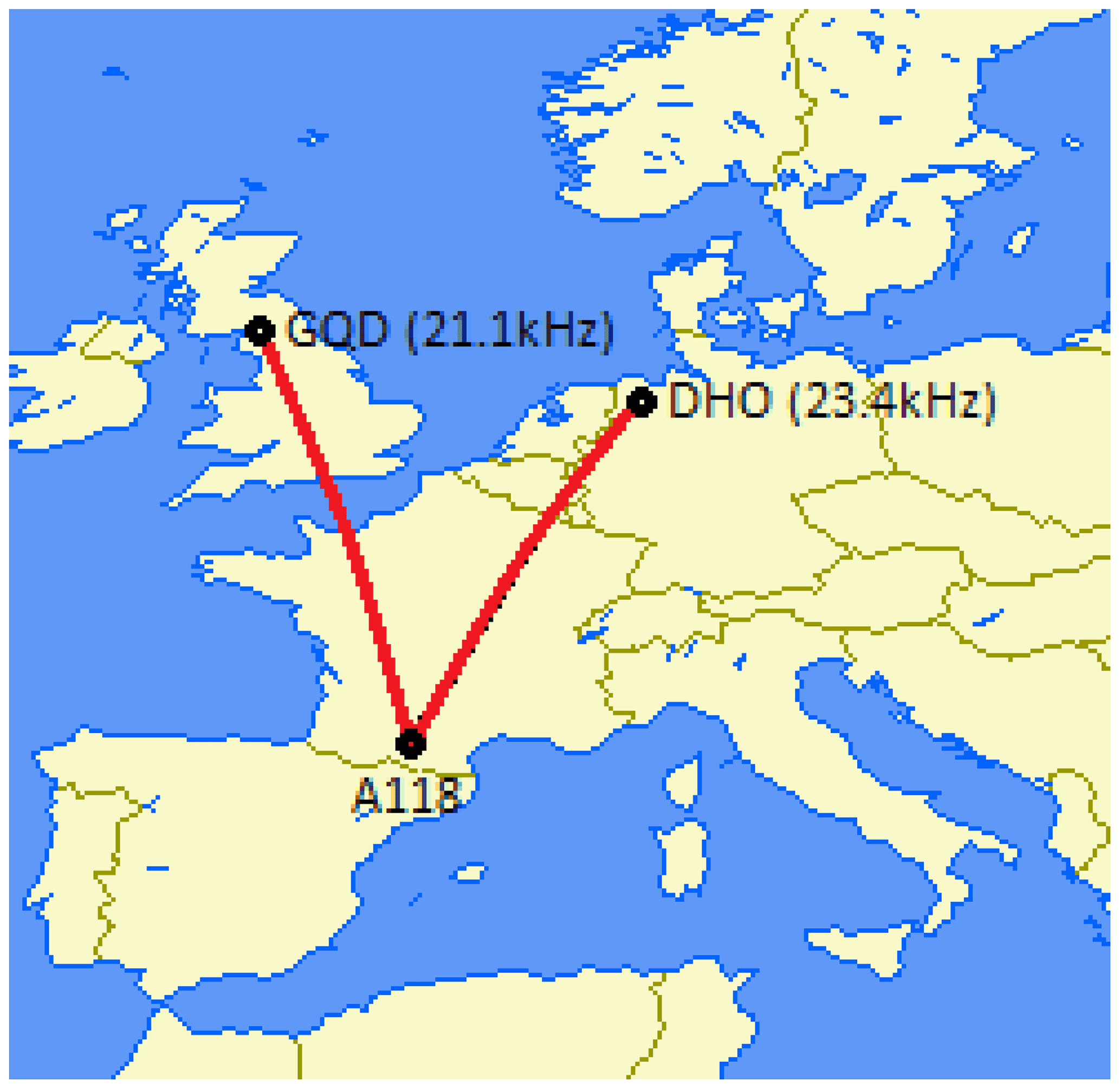
Figure 1 VLF signal propagation paths (DHO-A118 and GQD-A118) used in the study. Map adopted from the A118 channel; details at https://sidstation.loudet.org/channels-details-en.xhtml (last access: 18 May 2022).

We consider the TRGCP VLF data for the extended intervals 16 through 31 September 2011 and 22 October through 5 November 2011 which included the geomagnetic storm sub-intervals of interest on 17 September, 26–27 September, 25 October and 1 November 2011. The MBSR and MASS indices, as previously described, are the respective 2 to 4 h (dependent on signal quality or season, e.g. winter/summer) mean VLF signal amplitudes measured before local sunrise and after local sunset, whereas the MDP index is the peak signal amplitude measured near local noon. The frequency and power for the DHO and GQD transmitters can be considered constants in our analysis, whereas the received signal strength at A118 is subject to the path-integrated effect of attenuation due to the structure of the D region within the EIWG and the impact of atmospheric absorption. Figure 2 includes several examples of the diurnal variation in VLF signal strength for the DHO-A118 TRGCP. Times are referenced to Universal Time (UT), which is essentially local time of day at the A118 receiver site. The top trace is a rather well-behaved sample where the MBSR, MASS and MDP indices can be readily determined. Also shown in this top trace are the signal effects of the sunrise and sunset terminators, denoted as SRT and SST, respectively, which transit the TRGCP and are generally understood in terms of VLF-mode theory (Wait, 1960). However, not all diurnal traces are so well behaved. The middle example in Fig. 2 shows the transient effect of a solar flare on the VLF amplitude, which in this case would be classified as a SID and, more specifically, as a sudden enhancement of the signal strength of atmospherics (SEA) in accordance with Lincoln (1961). The lower trace includes an example of a “pseudo-SRT”, which illustrates the complicating effect of terminator-related modal interference along the TRGCP (Chand and Kumar, 2017). Relatedly, the evening-side SST signatures in the middle and lower traces are rather ambiguous, which, again, may be due to modal interference. The gist of these comments is to highlight the deleterious nature of VLF radio-wave propagation as a complicating factor in deriving the MBSR, MASS, MDP, SRT and SST indices. In previous work (Nwankwo et al., 2016, 2020, 2022), we have discussed how these factors can be effectively addressed and the somewhat subjective nature of the determination.

The examples in Fig. 2 clearly illustrate that VLF TRGCP propagation within the EIWG is affected by the dynamics of the ionosphere and, to a lesser extent, the thermosphere. The “classic” quantifications of the VLF reflection height, H^′ and sharpness, b (after Wait and Spies, 1964), are useful tools for assessing the local D-region response to solar-induced perturbations, for example SIDs, EPP, solar eclipses and geomagnetic storms as well as non-solar phenomena such as gravity waves and lightning (Silber and Price, 2017). For the TRGCP dataset at hand the received VLF amplitude reflects the integrated state of the traversed ionosphere along the signal path. In this regard we believe that the MBSR, MASS, MDP, SRT and SST indices provide a simpler yet more comprehensive set of metrics for assessing VLF TRGCP radio-wave propagation, particularly in the aftermath of a geomagnetic storm. By comparing and contrasting the changes in these indices for pre-storm versus storm time intervals, we hope to facilitate the development of a more comprehensive D-region specification that can be integrated into an empirical ionospheric model such as the IRI.

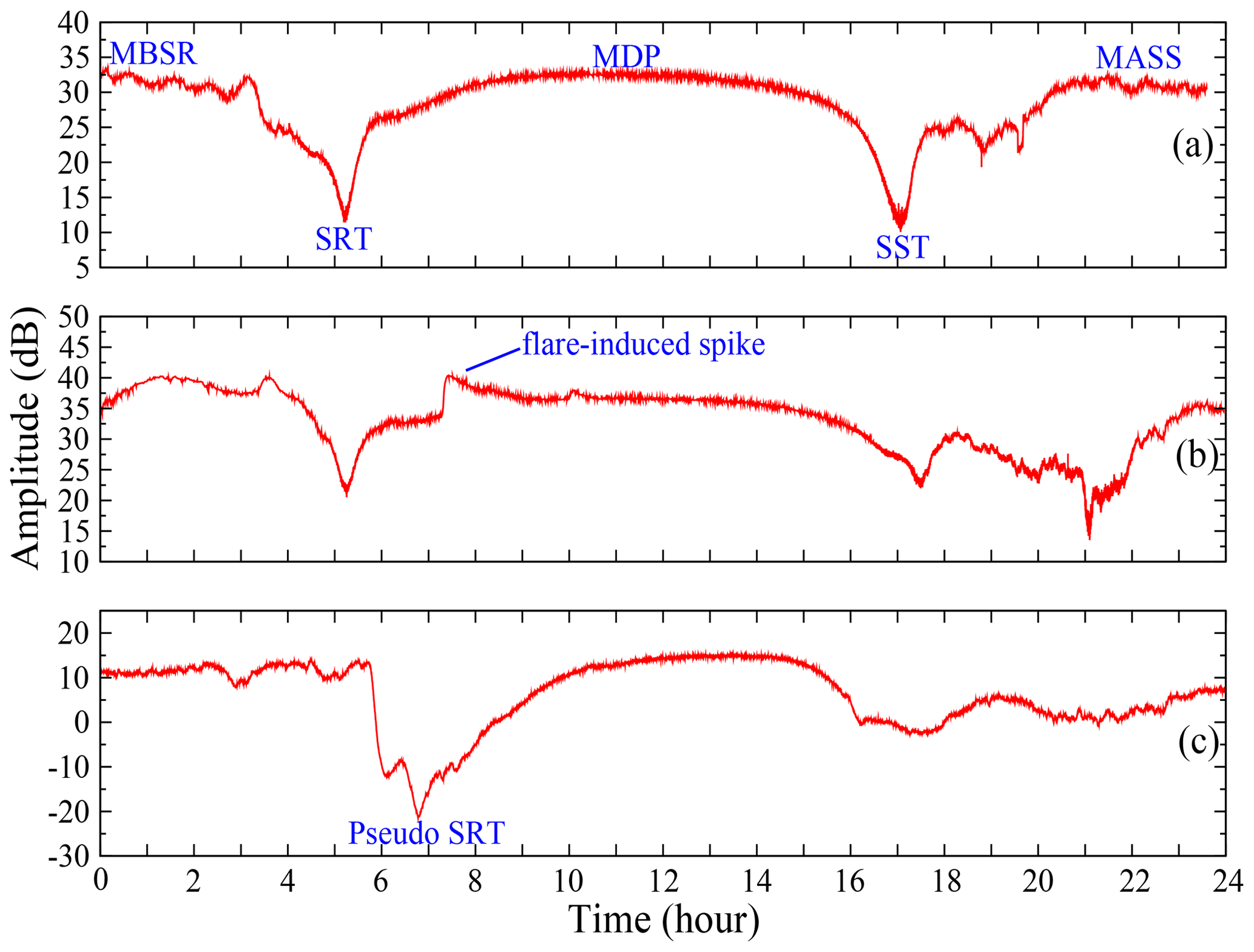
Figure 2 Diurnal VLF signal amplitude signatures (from the DHO-A118 propagation path) showing analysed signal metrics.

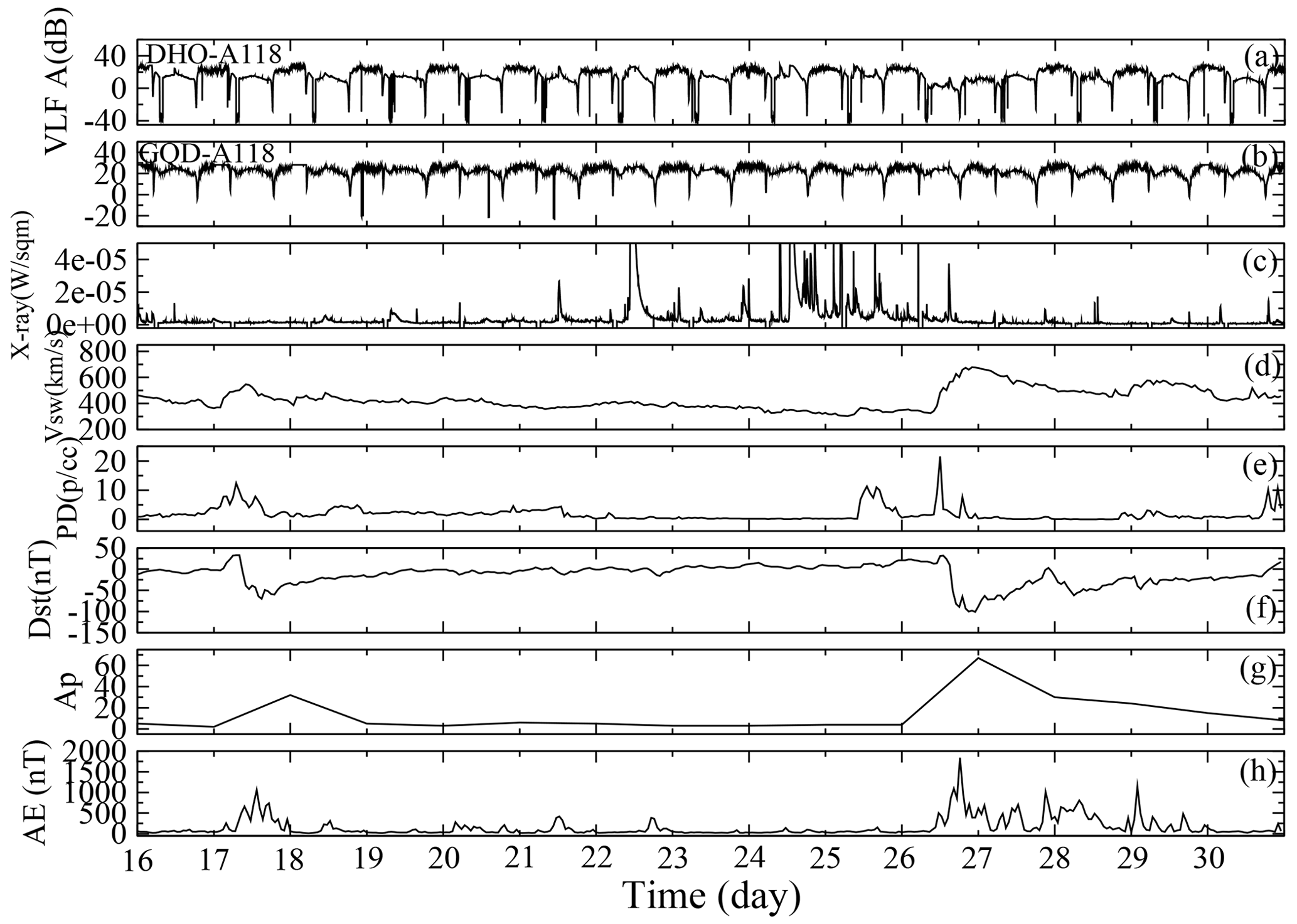
Figure 3 (a) Diurnal VLF amplitude for DHO-A118 and (b) GQD-A118 propagation paths, (c) daily variation in X-ray flux output, (d) solar wind speed (V_sw), (e) solar particle density (PD), (f) disturbance storm time (Dst), (g) planetary Ap, and (h) auroral electrojet (AE) indices during 16–30 September 2011.

3 Results and discussion

3.1 Analysis of VLF amplitude variations during intervals of geomagnetic storms

Figure 3 is a composite plot including the diurnal variation in VLF amplitudes for the (a) DHO-A118 and (b) GQD-A118 propagation paths plus the daily variation in the (c) solar X-ray flux output, (d) solar wind speed (V_sw), (e) solar wind PD, (f) Dst, (g) planetary geomagnetic Ap and (h) auroral electrojet (AE) indices during 16–30 September 2011. Four storm conditions occurred during this extended period, including an isolated storm of moderate intensity on 17 September (Dst $=-\mathrm{60}$) and consecutive storms on 26 September (Dst $=-\mathrm{101}$), 27 September (Dst $=-\mathrm{88}$) and 28 September (Dst $=-\mathrm{62}$), presumably driven by the significant increase in V_sw and PD on 17 September and 26 September (Fig. 3a–f). However, the main reference storms are those of 17 September and 26 September. The variation of the AE (especially between 26 September and 29 September) appears to be consistent with storm-related high-intensity, long-duration continuous AE activity events (HILDCAAs) during which “fresh energy was presumably injected” into the magnetosphere (Tsurutani et al., 2011). A notable drop occurred in the DHO-A118 VLF signal level on 26 September around midday, coincident with a relatively intense storm with Dst of −101 (Fig. 3a). This scenario (signal strength decrease) has been associated with storm-induced variations in energetic electron precipitation flux (Kikuchi and Evans, 1983; Peter et al., 2006). During a geomagnetic storm, the current system in the ionosphere and the energetic particles precipitating into the ionosphere can influence the density and distribution of density in the atmosphere (NOAA, 2016). The characterised metrics (e.g. MBSR, MDP, MASS, SST and SRT) of the VLF signal amplitude make it easier to study the behaviour of the signal during the storms. We therefore monitor trends of the signal variation in the analysis to follow for possible identification of storm-induced variation in the signal due to lower ionosphere responses.

Figure 4 shows daily mean fluctuation of Dst and AE and variations in the VLF midday signal amplitude peak (MDP), mean signal amplitude before local sunrise (MBSR), mean signal amplitude after sunset (MASS), sunrise terminator (SRT) and sunset terminator (SST) for the (a) DHO-A118 and (b) GQD-A118 propagation paths from 16 to 30 September 2011. In the GQD-A118 propagation path (Fig. 4a), we observed a dipping of the MDP on 17 September (extending to 20 September) as well as dipping of the MASS on 17 September but an increase in the MBSR, SRT and SST. Following the recurrent storms between 26 and 28 September, we observed dipping of the MDP on 26 September (extending to 29 September). The slight increase in the signal (MDP) on 28 September appears to be due to the significant flare activity (three C-class and one M-class), suggesting an increase in both the instantaneous and background X-ray flux output that usually results in an increase in signal amplitude (as depicted in Fig. 2b). High flare activity can “overshadow” the signal's response to geomagnetic storms when the event coincides with storm time (Nwankwo et al., 2016). There is also a significant dipping of all the signal metrics (MDP, MBSR, MASS, SRT and SST) on 27 September. We note dipping of the MBSR on the days following the main (reference) storms on 18 and 27 September. Since the events occurred after dawn (around midday), the post-storm ionospheric effects are expected well into the day following the storm. This trend (post-storm day signal dip) suggests that the signals dipped in response to continuous driving of the ionosphere on the days following the events. However, such a response also depends on the characteristics of the signal propagation path. In the DHO-A118 propagation path, dipping of the MDP, MBSR, SRT and SST occurred on 17 September, while the MDP, MASS and SST also decreased on 26 September. The MASS and SRT maintained the pre-storm day values of 16 and 25 September, respectively. While the MBSR increased slightly on 26 September (main storm day), there is a significant dipping of the signal following the recurrent storm of 27 September.

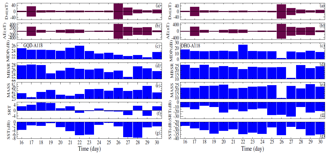
Figure 4 Daily deviations of (a) Dst, (b) AE, (c) variations in the peak value of midday signal amplitude (MDP), (d) mean signal amplitude before local sunrise (MBSR), (e) mean signal amplitude after sunset (MASS), (f) variation in sunrise terminator (SRT), and (g) sunset terminator (SST) for the GQD-A118 (left column) and DHO-A118 (right column) propagation paths from 16 to 30 September 2011.

Figure 5 depicts the diurnal VLF amplitude for the (a) DHO-A118 and (b) GQD-A118 propagation paths, daily variation in (c) X-ray flux output, (d) V_sw, (e) PD, (f) Dst, (g) Ap and (h) AE indices from 22 October to 5 November 2011. This period was associated with a severe storm with the main phase on 25 October (Dst $=-\mathrm{132}$) and consecutive storms on 1 November (Dst $=-\mathrm{71}$) and 2 November (Dst $=-\mathrm{57}$), presumably driven by the highly variable V_sw and PD (Fig. 5d–e). It has been shown that the capability of a given value of the solar wind electric field (SWEF) to create a Dst disturbance or geo-efficiency is enhanced by high solar wind density (Weigel, 2010; Tsurutani et al., 2011). Variation of the AE between 30 October and 3 November also appears to be consistent with a HILDCAA event (Fig. 5h). The DHO-A118 VLF signal level on 25 October around midday also showed a visible reduction following the intense storm condition with a Dst of −132 (Fig. 5a). VLF signal data for the GQD-A118 propagation path are not available from 12:00 on 25 October to 18:00 on 26 October (Fig. 5b).

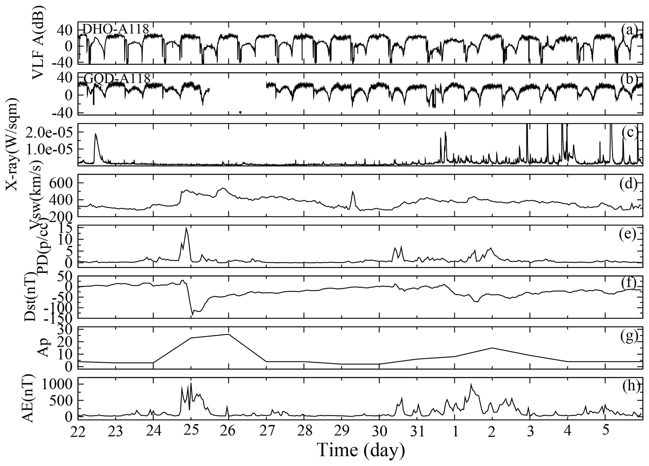
Figure 5 (a) Diurnal VLF amplitude for the DHO-A118 and (b) GQD-A118 propagation paths, (c) daily variation in X-ray flux output, (d) solar wind speed (V_sw), (e) solar particle density (PD), (f) Dst, (g) planetary Ap, and (h) AE indices from 22 October to 5 November 2011.

Figure 6 plots the daily deviations of Dst and AE and variations in the MDP, MBSR, MASS, SRT and SST for the (a) DHO-A118 and (b) GQD-A118 propagation paths from 22 October to 5 November 2011. Although data for the GQD-A118 propagation path during 25 and 26 October were inadequate for the present analysis, we did observe a dipping of the MBSR on the main storm day (25 October). Dipping of the MDP, MASS and SST occurred on 1 November and those of MBSR, MASS and SRT on 2 November, following the consecutive storms. In the DHO-A118 propagation path, we observed dipping of the MDP, MBSR, MASS and SRT on 25 October, dipping of the MDP, MBSR, MASS and SST on 1 November and dipping of the MBSR and SRT on 2 November. Similar to the first case (Figs. 4 and 5), we note the numerous flare events on 2 November (up to seven C-class and one M-class) that may have induced a spike in the MDP on the day in both the GQD-A118 and DHO-A118 propagation paths. Although dipping of the MDP signal (following storm events) has shown considerable consistency across the cases presented so far, the MBSR and MASS (in particular) appear to be influenced by storm occurrence time and the high variability or fluctuation of the dusk-to-dawn ionosphere (and signal) (Nwankwo et al., 2016). However, presenting a consistency across a substantial number of cases is vital to the conclusion of this work. We, therefore, analysed 15 additional storm cases between September 2011 and October 2012 in order to obtain a statistically significant set of observations. The 15 storm cases are presented in Table 1.

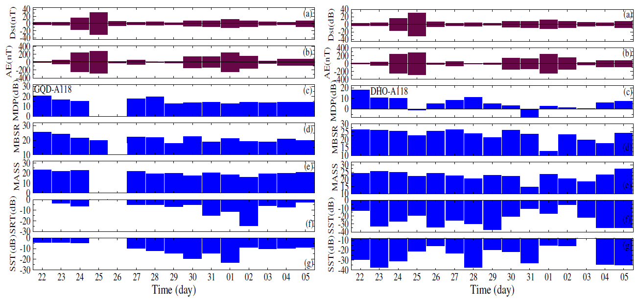
Figure 6 Daily deviations of (a) Dst and (b) AE and (c) variations in MDP, (d) MBSR, (e) MASS, (f) SRT, and (g) SST for the GQD-A118 (left column) and DHO-A118 (right column) propagation paths from 22 October to 5 November 2011.

Table 1 Summary of the 15 analysed geomagnetic storm events.

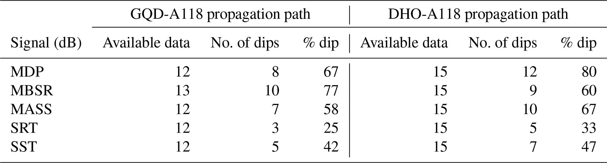
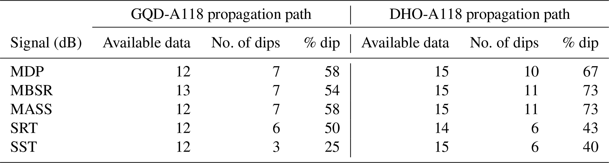
In Fig. 7, we show Dst deviations (σ_Dst) and trends in variation of the MDP, MBSR, MASS, SRT and SST signals on the day before the storm (blue bar), the storm day (red bar) and after the storm day (brown bar) for the 15 selected storm cases in the (a) GQD-A118 and (b) DHO-A118 propagation paths. σ_Dst is the measure or extent of daily fluctuation in measured values of Dst. We recognised the 3 consecutive days as day before event (BE), during event (DE) and after event (AEv). A missing index indicates an absence of data. It should be noted however (for this analysis) that these events were separate events and not continuous events. In the GQD-A118 propagation path, about 8 of 12 MDPs, 10 of 13 MBSRs, 7 of 12 MASSs, 3 of 12 SRTs and 5 of 12 SSTs showed dipping features, while 12 of 15 MDPs, 9 of 15 MBSRs, 10 of 15 MASSs, 5 of 15 SRTs and 7 of 15 SSTs showed dipping in the DHO-A118 propagation path. These values correspond to 67 %, 77 %, 58 %, 25 % and 42 % dipping in the GQD-A118 propagation path and 80 %, 60 %, 67 %, 33 % and 47 % dipping in the DHO-A118 propagation path. The signal levels along with the percentage dip are presented in Table 2. The MDP signals (in both propagation paths) generally show a tendency for dipping following geomagnetic storm conditions. However, we also observe a few cases of increase in the MDP during separate events in each of the propagation paths (e.g. events 4 and 7 in GQD-A118 and 9 in DHO-A118) as well as coincident increases occurring in both propagation paths during the same event (e.g. events 3 and 12). While the probable reason for this coincidence is suggestive of factors such as propagation characteristics and/or X-ray flux-induced spikes in amplitude (e.g. significant X-ray output during events 3 and 7 in Fig. 8c), further investigation into why this characteristic exists will be pursued. In the meantime, we analysed variations in X-ray flux output and geomagnetic indices during events 3 and 12 to better interpret the prevailing ionospheric conditions at the time.

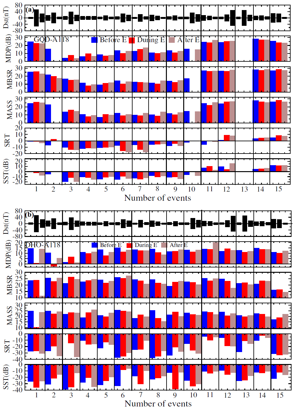
Figure 7 Dst deviation (or fluctuation) and variations in MDP, MBSR, MASS, SRT and SST signals 1 d before, during and after each of the 15 events for the GQD-A118 and DHO-A118 propagation paths. Note that each Dst bar represents the deviation (σ) corresponding to the VLF amplitude before, during and after the selected events (storm) as listed in Table 1 and shown in Fig. 8. The events are selected (for the intervals shown in Fig. 8) and are not continuous.

Table 2 Summary of the trend in dipping of the signals' metrics during 15 geomagnetic storm cases in the (a) DHO-A118 and GQD-A118 propagation paths.

In Fig. 8, we present the diurnal VLF amplitudes for the (a) DHO-A118 and (b) GQD-A118 propagation paths, daily variation in (c) X-ray flux output, (d) V_sw, (e) PD and (f) Dst indices for a day before and after each of the 15 storms. Data showed (Fig. 8c, f) the occurrence of an M-class flare in association with the storm on 22–23 January 2012 (event 3 on 21 January), both events having near-corresponding peaks. This scenario suggests an enhancement of both the instantaneous and background X-ray flux output (as stated earlier) that may have caused an increase (or spike) in the signal level and thus probably overshadowed geomagnetic effects on the signal. While this explanation may be argued for events 1 (25–27 September 2011) and 6 (6–8 March 2012), it should be noted that the flare events started well before the storms and continued until the storm time (in each case), suggesting an established increase in the overall background X-ray before the storms. Hence, it is possible for a storm-induced dipping to manifest under such a condition. However, further investigation is encouraged, which is beyond the scope of this work. For event 12 (from 15 to 17 July 2012), we observed that the peak of the storm (that commenced by midnight on 16 July) was on 17 July (recognised as AEv). Therefore, any geomagnetic influence on the signal (e.g. dipping) is expected on 17 July (or after) and not 16 July, hence the dipping of the AEv signal (on 17 September) in the DHO-A118 propagation path.

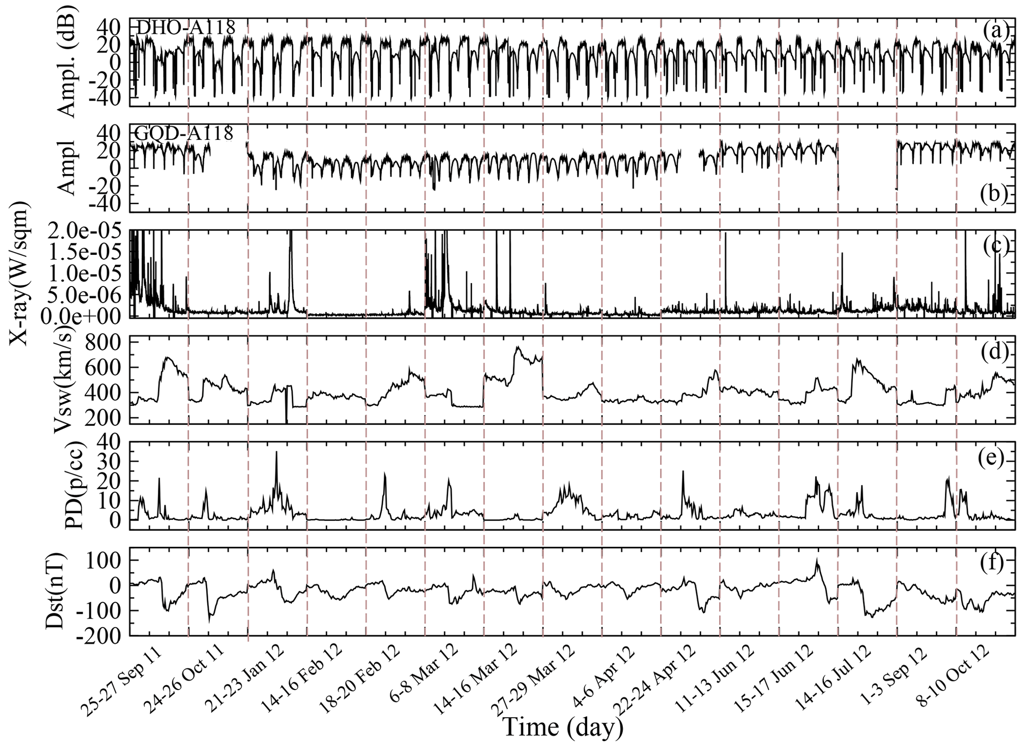
Figure 8 Diurnal VLF amplitude for the (a) DHO-A118 and (b) GQD-A118 propagation paths, daily variation in (c) X-ray flux output, (d) V_sw, (e) PD, and (f) Dst indices for a day before and after each of the 15 storms.

Figure 9 shows Dst deviation (fluctuation) and 2 d mean variations of MDP, MBSR, MASS, SRT and SST signals before, during and after each event for the (a) GQD-A118 and (b) DHO-A118 propagation paths. This analysis is important for corroborating the result presented in Fig. 7, because the data selection criteria differ from those of Fig. 7 in some ways. While BE, DE and AEv represent data for 3 consecutive days with reference to the event's day (DE) in the former analysis (presented in Fig. 7), each abbreviation (BE, DE or AEv) represents a relatively quiescent 2 d mean amplitude before and after DE (but not necessarily in succession to/after DE). However, it should be noted that, due to the data averaging (2 d), a “pronounced” increase or dipping in the signals (comparable to those in the former analysis, Fig. 7) is not expected. Another important data selection criterion for this analysis is a relatively geomagnetic quiet day BE and AEv with respect to DE.

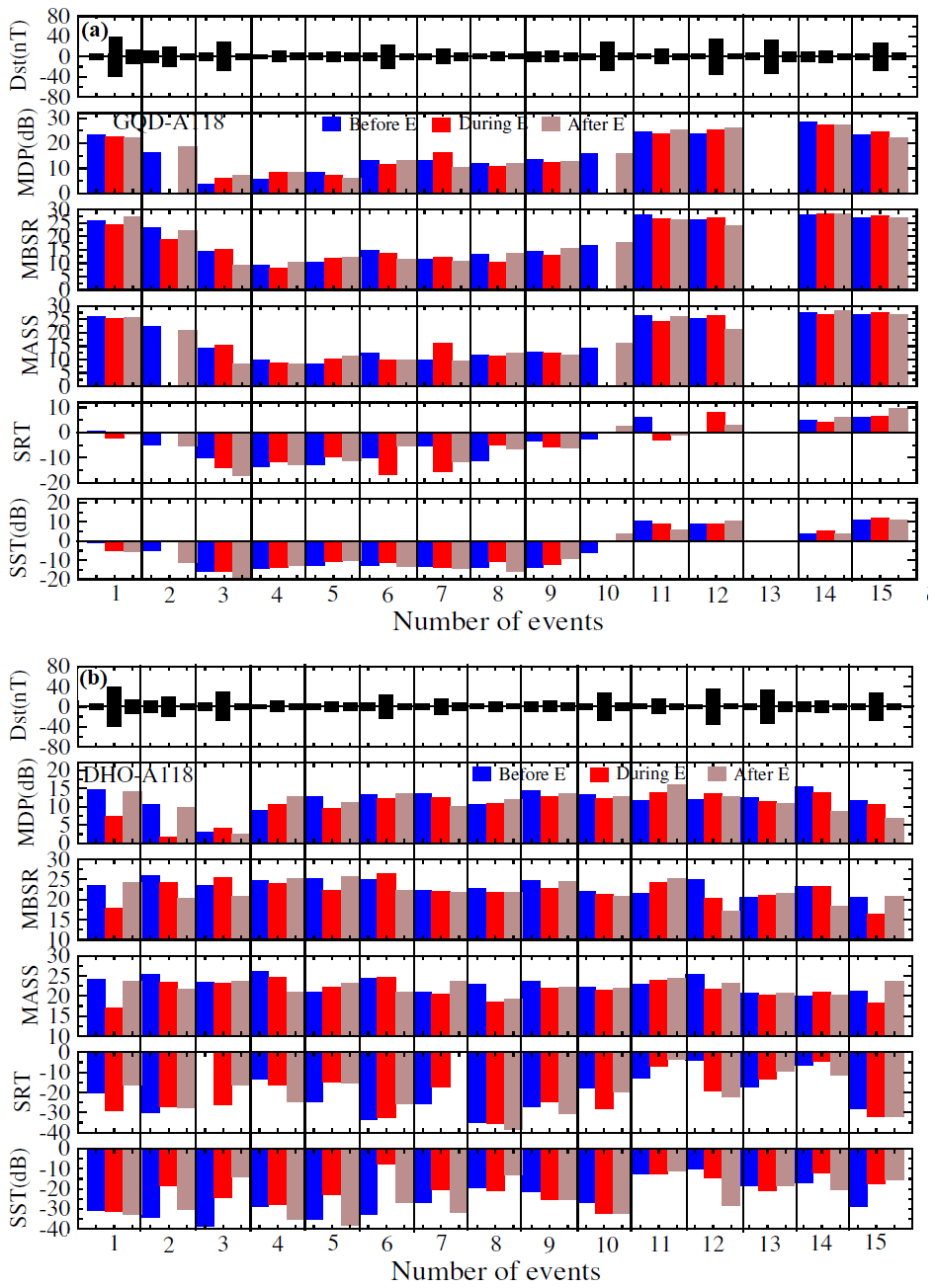
Figure 9 Dst deviation and 2 d mean variations of MDP, MBSR, MASS, SRT and SST signals before, during and after each event for the GQD-A118 and DHO-A118 propagation paths.

In the GQD-A118 propagation path, 7 of 12 MDPs, 7 of 13 MBSRs, 7 of 12 MASSs, 6 of 12 SRTs and 3 of 12 SSTs showed dipping following the storms, while 10 of 15 MDPs, 11 of 15 MBSRs, 11 of 15 MASSs, 6 of 14 SRTs and 6 of 15 SSTs showed dipping in the DHO-A118 propagation path. These values correspond to, respectively, 58 %, 54 %, 58 %, 50 % and 25 % dipping in the GQD-A118 propagation path and 67 %, 73 %, 73 %, 43 % and 40 % dipping in the DHO-A118 propagation path. The signal levels along with the percentage dip of the signals are presented in Table 3. In general, the trend of variation of the signal metrics reflected the prevailing space weather-coupled effects in the lower ionosphere. The MDP signal appears to be more responsive to geomagnetic perturbations (58 % and 67 % (67 % and 80 % for 1 d mean analysis) in the respective propagation paths shown in Figs. 7 and 9) than other signal metrics. However, the 2 d mean analysis showed improvement in MBSR and MASS (73 %) of the DHO-A118 propagation path, thereby reenforcing the responsiveness of this propagation path to geomagnetic storm impacts. While the mechanism of VLF amplitude (and/or MDP) response to flare-induced SIDs is well understood (see Sect. 1.3 of Nwankwo et al., 2016), the mechanism of the transient response of the signal to geomagnetic storming is not well developed. We speculate that the dipping response of the MDP may be related to (i) a positive storm effect, which affects, albeit to a small extent, the attenuation of the VLF radio waves (Fagundes et al., 2016), (ii) adjustment of the D layer to storm-driven energy input (McPherron, 1979), (iii) precipitation of energetic electrons (Rodger et al., 2010, 2012; Naidu et al., 2020) and/or (iv) charge exchange between surrounding ionospheric regions (Tatsuta et al., 2015). Since the processes are gradual (when compared with the SID scenario) and originate from the magnetosphere, it is not likely that a remote spike would occur in the diurnal signal (as observed during the flare condition). One other likely reason for the observed dipping characteristic is the modification of the chemistry of the D region by storm precipitation of SEPs (Turunen et al., 2009), since chemistry (mainly NO) controls the quiescent D region (Siskind et al., 2017).

Nwankwo et al. (2016) noted the existence of pseudo SRT and/or SST sometimes exhibited by diurnal VLF signal (see Fig. 2c) as a drawback in SRT and SST analysis. This anomaly is due to the secondary destructive interference pattern in signals and/or occurrence of solar flares during sunrise/sunset (Sandip Chakrabarti, personal communication, 2016). The authors concluded in their study that the post-storm SRT and SST variations do not appear to have a well-defined trend associated with the storm effect based on the approach used in the analysis (Nwankwo et al., 2016). In this work, we considered the “first” SRT and SST values (in the event of a pseudo-terminator) during analysis of the signal metrics. A rise in SRT and SST amplitude under geomagnetic storm conditions appears to occur more than otherwise in both propagation paths. We found a respective dipping of 50 % and 25 % (43 % and 40 %) of the SRT and SST. Storm-induced disturbances may not have a significant influence on these metrics (SRT and SST), and since the sunrise and sunset signatures relate to mode conversion in the VLF propagation path, it might imply that the D-region density is not a significant contributor to this effect. It is important to note that, of the two propagation paths used in this study, the DHO-A118 signal appears to be more sensitive to geomagnetic storm-induced magnetosphere–ionospheric dynamics. We do not expect a “perfect” consistency in signal trend and variations across all cases, because the individual effects of solar and other forcing mechanisms (including those of lithospheric and atmospheric sources) on the ionosphere are difficult to estimate (Kutiev, 2013; Nwankwo et al., 2016). This scenario can also cause non-linear coupling processes and consequent significant fluctuations in radio signals.

Table 3 Summary of trends in 2 d mean signal dipping following 15 geomagnetic storm cases in the DHO-A118 and GQD-A118 propagation paths.

3.2 Investigating the state of the ionosphere over the propagation paths of the VLF signals

Here, we study the state of the ionosphere over the two VLF propagation paths using the virtual heights (h'E, h'F1 and h'F2) and critical frequencies (foE, foF1 and foF2) of the E and F regions obtained from two ionosonde stations near the GQD and DHO transmitters. Although we made an effort to obtain data from stations near each transmitter/receiver and at the mid-point, we found no ionosonde station at the mid-point, and the nearest station to the receiver (Tortosa) has no data for the period/intervals under study. However, to make up for this dearth of data, we will complement the analysis with the results in the extended study that utilised the GNSS data in the region (e.g. Nwankwo et al., 2022). Details of the ionosonde stations used in this study are provided in Table 4. We treat Chilton station as nearest to the GQD transmitter and Juliusruh station as nearest to the DHO transmitter. Tortosa station is closest to the A118 transmitter but has no data for the intervals. We obtained and calculated the daytime (08:00–15:00) mean values and standard deviations (σ) of the parameters and then analysed them for the storms of interest (on 17 and 26 September and 1 November) within the intervals 16–19 and 25–28 September and 29 October to 2 November 2011. We exclude analysis of the 25 October storm because the data for this interval are inadequate.

Table 4 Ionosonde stations near the VLF transmitters and receiver and/or propagation paths.

Figure 10 shows the daily mean and standard deviation (SD or σ) of foF2, foF1, foEs, foE, h'F2, h'F, h'Es and h'E from 16 to 17 September 2011 for Chilton and Juliusruh stations. We compared the pre-storm day (blue broken line) values with the storm day (red broken line) values. At Chilton station (near the GQD transmitter), results show significant increase and/or fluctuation (increase in SD) in foF2 and a decrease (with significant fluctuation) in foF1 on the storm day, 17 September. The height of the E and F regions (h'F2, h'F, h'Es and h'E) significantly increased following the storm. A similar pattern of variations was observed at Juliusruh station. foF2 and foF1 increased (and/or fluctuated) significantly, as well as h'F2, h'F, h'Es and h'E. Values of foEs decreased, while foE remained unaffected in both stations. Also, there appear to be a sustained post-storm increase and/or fluctuations of the parameters on 18 September, suggesting a continuous driving of the ionosphere by the storm.

Figure 10 Daytime mean variations and standard deviation (SD) of foF2, foF1, foEs, foE, h'F2, h'F, h'Es and h'E from 16 to 17 September 2011 for Chilton and Juliusruh stations. The blue broken line represents the pre-storm day values, while the red broken line represents the storm day values of the ionospheric parameters.

Figure 11 shows the daytime mean variations and SD of foF2, foF1, foEs, foE, h'F2, h'F, h'Es and h'E from 25 to 28 September 2011 for Chilton and Juliusruh stations. The storm during this interval (on 26 September) was well developed (with Dst up to −101 nT) and larger than the 17 September event. The result of this analysis shows a slight increase in foF2 and foF1 but a decrease in foEs and foE for Chilton station. The height of F2 (h'F2) decreased (by 6.90 km), while those of F, Es and E increased on the storm day, 26 September. Near the DHO transmitter (Juliusruh station), there is an anti-correlated variation in the critical frequencies of the E and F regions: a depression of foF2 and foF1 but an increase in foEs and foE (when compared with the scenario at Chilton station). The height of the F2, F and E regions increased by 47.89, 16.08 and 9.14 km, respectively (which are so far the largest increase in the parameters), while the height of the Es region decreased by 0.16 km (see Table 5).

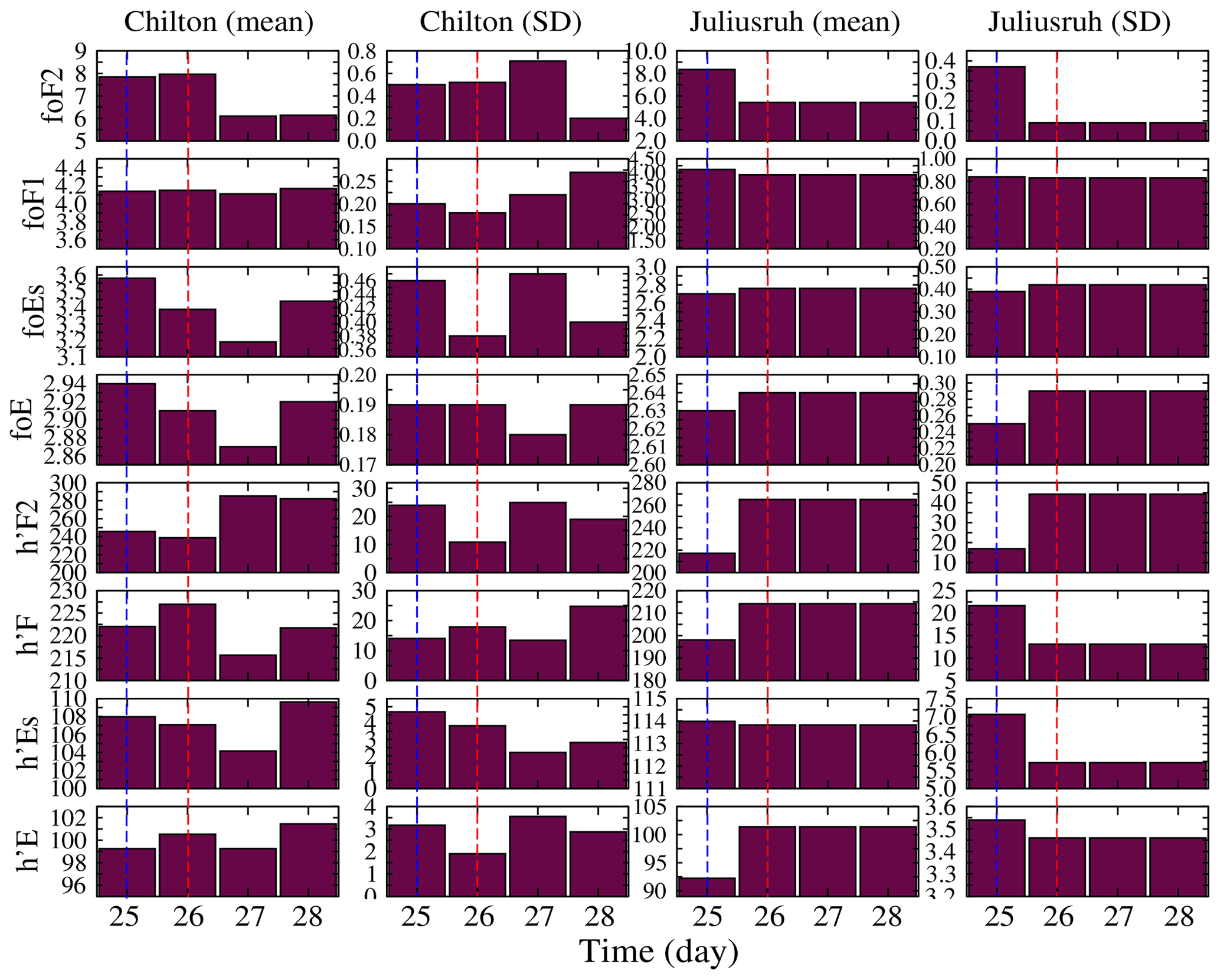
Figure 11 Daytime mean variation and SD of foF2, foF1, foEs, foE, h'F2, h'F, h'Es and h'E from 25 to 28 September 2011 for Chilton and Juliusruh stations.

Figure 12 shows the daytime mean variation and SD of foF2, foF1, foEs, foE, h'F2, h'F, h'Es and h'E from 29 October to 2 November 2011 for Chilton and Juliusruh stations. This interval is of interest because of the fluctuation in geophysical parameters during the days preceding the storm. We include this interval to investigate the coupling effect of this extended period (30–31 October) of geomagnetic disturbances preceding the storm on 1 November. It appears that energy began building up in the magnetosphere–ionosphere system after the first significant spike in V_sw around 07:00 on 29 October (and subsequent increase on 30 October) and PD around 10:00 on 30 October until around 10:00 on 1 November, when the storm was triggered following a sudden increase in V_sw and southward turning of the B_z (Nwankwo et al., 2020). Here, we compare the parameter level on the relatively quiet day (29 October) with those of the storm day (on 1 November), since the 2 days preceding the storm were significantly disturbed. The result shows significant increases in foF2 and foF1 at Chilton station. Like the 17 September storm scenario, values of foEs decreased, while foE remained unaffected for this station. h'F2 decreased, while h'F, h'Es and h'E showed significant increase. At Juliusruh station only the critical frequency of the F2 region increases, while those of F1, Es and E decreased. However, the increase and/or fluctuation of the parameters were significant (in most cases) during the disturbed days (30 and 31 October) preceding the storm, suggesting responses of the E and F ionosphere regions (coupled to the D region) before the storm commencement (as a result of increased geomagnetic activity on the days). We present a summary of the storm day variations in h'F2, h'F, h'Es and h'E for the two stations in Table 5.

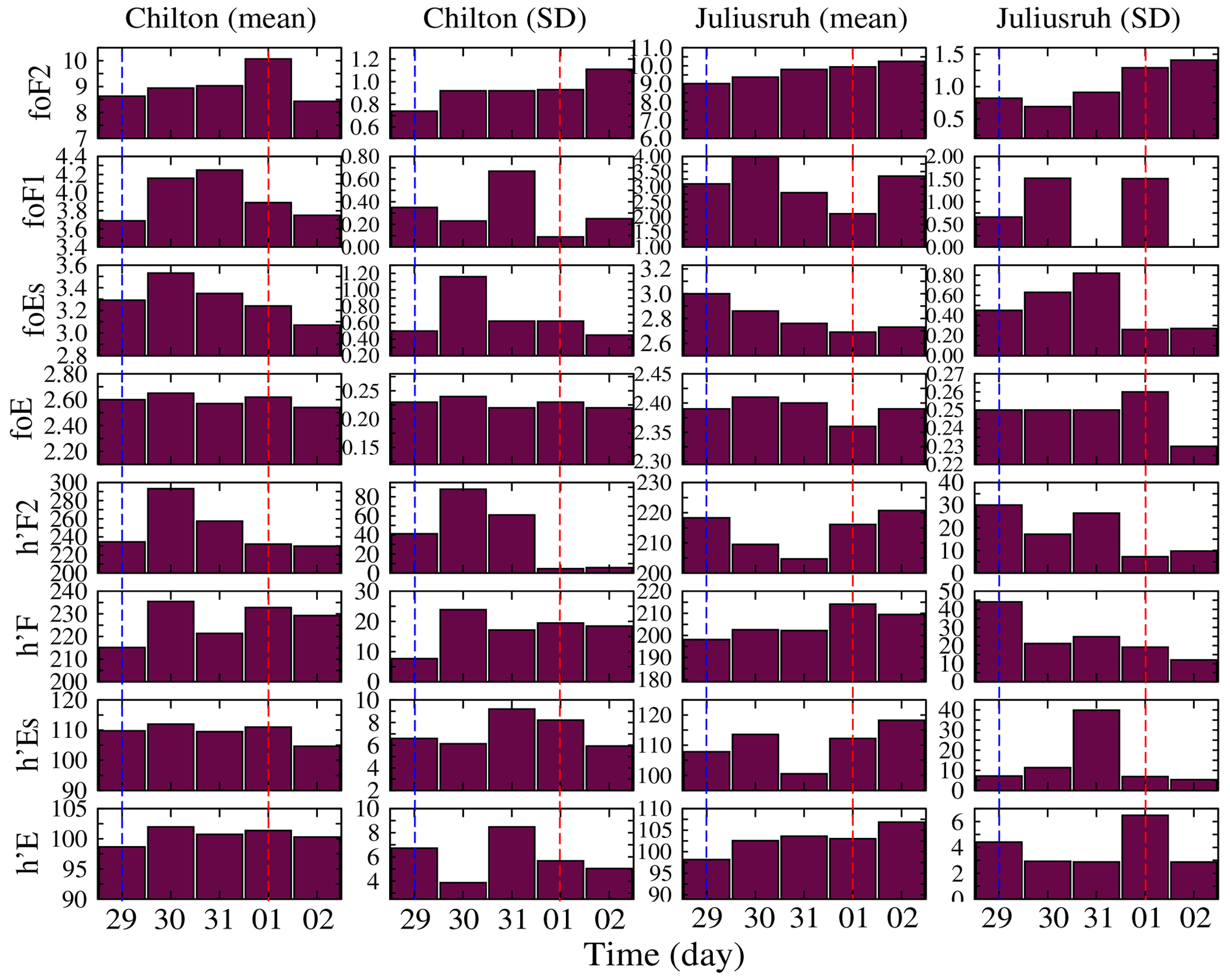
Figure 12 Daytime mean variation and SD of foF2, foF1, foEs, foE, h'F2, h'F, h'Es and h'E from 29 October to 2 November 2011 for Chilton and Juliusruh stations.

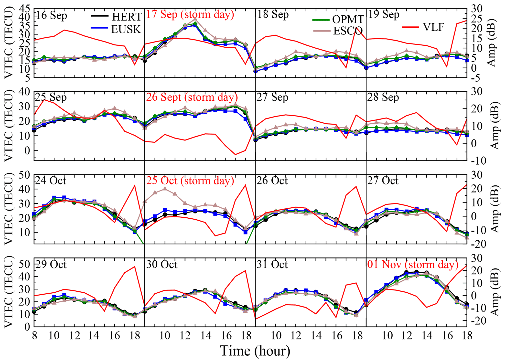
Figure 13 Daytime variation in VLF amplitude (red line plot) for the DHO-A118 propagation path, together with VTEC values obtained from HERT (black line), EUSK (blue line), OPMT (green line) and ESCO (brown line) stations across some locations in Europe during 16–19 and 25–28 September, 24–27 October and 29 October–1 November 2011 (from Nwankwo et al., 2022).

Table 5 Observed increase (or decrease) in h'F2, h'F, h'Es and h'E during the storms on 17 and 25 September and 1 November 2011.

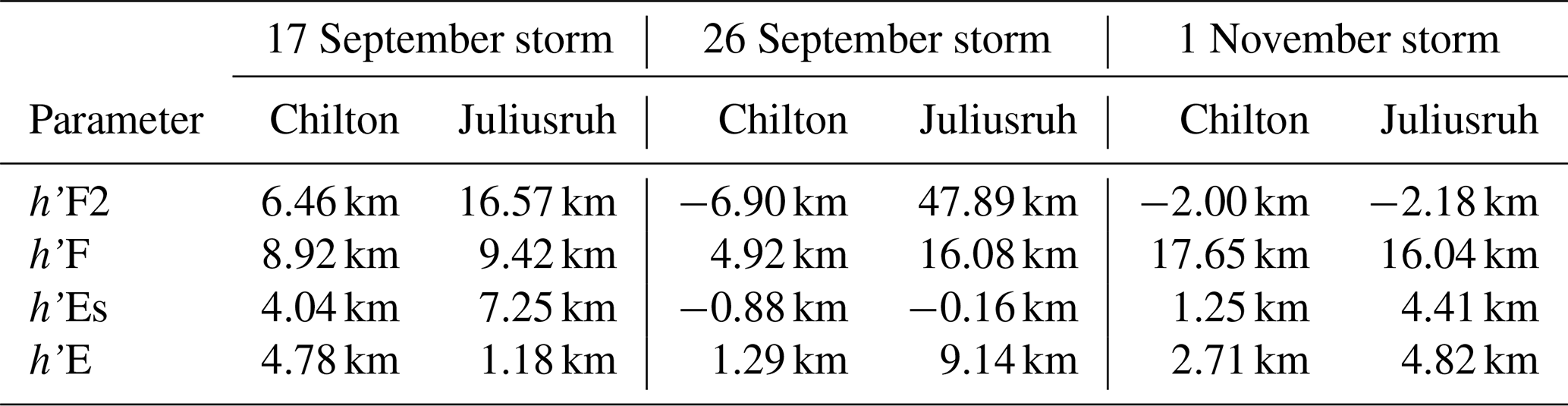
In summary, foF2, foF1, h'F2, h'F, h'Es and h'E generally showed significant increases and/or fluctuations near both transmitters (GQD and DHO) during the geomagnetic storms, whereas foEs and foE mostly decreased (but slightly increased in fewer cases) or remained unaffected. It appears that the observed storm-induced increases and fluctuations were largely sustained or further enhanced on the day (or days) following the event (post storm day), suggesting a continuous driving of the ionosphere by the storms and/or a substorm effect. Although the analysis for the 1 November storm scenario showed weak correlation, variations of the parameters reflected the coupled responses of the ionosphere to energy build-up ahead of storm commencement. Nwankwo and Chakrabarti (2018) reported significant depression and fluctuations of foF2 following significant geomagnetic disturbances and/or storms at high and mid latitudes and distortion in the quasi-periodic pattern of the parameter. Their inference was, however, based on a preliminary analysis from the result of a single ionosonde station. From this comparatively detailed analysis, it is clear that the reported depression of foF2 may occur during some (isolated) storms and locations, and should, therefore, not be treated as a global response. Negative storm effects (in which foF2 decreases) have also been reported (e.g. Blanch et al., 2013; Kane, 2005). In this analysis, the largest increase in h'F2, h'F, h'Es and h'E occurred in Juliusruh near the DHO transmitter (see Table 5). The ionosonde observations indicated that fluctuations in the reference heights appeared to be the dominant response of the E and F regions to geomagnetic storms, whereas attenuation of the VLF radio-wave signal strength was responsive to the storm-induced dynamics in the ionospheric D region. This observation is instructive in that the observed large ionosonde increase and the large amplitude decreases in the DHO-A118 propagation path signal may be related to coupled effects between the ionospheric regions but are also suggestive of strong storm responses (more intense) around/near the DHO transmitter or DHO-A118 propagation path. This result is in agreement with the recent findings reported in Nwankwo et al. (2022). Their study combined observed VLF amplitude variations with TEC/VTEC data obtained from multiple GNSS stations, including Euskirchen in Germany (EUSK), Hailsham in the UK (HERT), Paris in France (OPMT) and Naut Aran in Spain (ESCO), to investigate the ionospheric response to storms over some signal propagation paths during the same events. They showed and reported a simultaneous decrease in VLF amplitude and enhancement of electron density profiles near the DHO transmitter. In Fig. 13 we show the daytime variation in VLF amplitude (red line plot) for the DHO-A118 propagation path, together with VTEC values obtained from HERT (black line), EUSK (blue line), OPMT (green line) and ESCO (brown line) stations across some locations in Europe during 16–19 and 25–28 September, 24–27 October and 29 October–1 November 2011. HERT is closest to the GQD transmitter (about 508.12 km), EUSK is closest to the DHO transmitter (about 279.99 km), while ESCO is nearest to the receiver (about 90.47 km).

One clear observation (from Fig. 13) is the strong dipping (or reduction) of the daytime VLF amplitude and the simultaneous increase in VTEC values on the storm days in the DHO-A118 propagation path. We note the large increase in VTEC values for ESCO station located near DHO, especially during the 17 September and 25 October storms. This feature is in agreement with the findings of Choudhury et al. (2015), who reported that the receiver position electron density is the main factor influencing the VLF signal at ionospheric sunrise time during long-duration geomagnetic storms. It is also worth noting that the ancillary information of the timing, classification and location of associated solar flares, CMEs, SPEs, and timings for the SSCs showed that the strong storm intervals during which large dipping or decrease in DHO signal level occurred were associated with SPEs (see Table 5 in Nwankwo et al., 2022). The results of this effort that combined the diagnostics of the D, E and F regions (to probe the geostorm effects in the lower ionosphere) demonstrate that, despite the tenuousness of the coupling between the dayside upper- and lower-ionospheric regions, the adjoining regions of E and F play significant roles in driving the storm-induced dynamics of the D region and the associated observed responses of VLF radio waves within the context of solar–terrestrial coupling.

4 Conclusions

In this work we performed a diagnostic study of geomagnetic storm-induced disturbances that were coupled to the lower ionosphere in the mid-latitude D region using propagation characteristics of VLF radio signals. We characterised the diurnal signal into five metrics (i.e. MBSR, MDP, MASS, SRT and SST) and monitored the trend in variations of the signal metrics for up to 20 storms between September 2011 and October 2012. The goal of the analysis was to understand deviations in the signal that were attributable to the storms. Up to five (5) storms and their effects on the signals were studied in detail, followed by statistical analysis of 15 other cases. Our results showed that the MDP exhibited characteristic dipping in about 67 % and 80 % of the cases in the GQD-A118 and DHO-A118 propagation paths, respectively. The MBSR showed respective dipping of about 77 % and 60 %, while the MASS dipped by 58 % and 67 %. Conversely, the SRT and SST showed respective dipping of 25 % and 33 % and 42 % and 47 %, favouring the rise of the signals following storms. The MDP consistently showed strong responses to the storms than the other metrics (followed by the MBSR and the MASS). Among other possible reasons outlined in this paper, we speculate that the responses were related to positive storm effects, resulting in an attenuation of the VLF radio waves. Of the two propagation paths examined in this study, we observed stronger dipping of the VLF amplitude of the DHO-A118 propagation path during the storms. To understand the state of the ionosphere over the propagation paths and examine how the upper ionosphere (E and F regions) might have affected VLF transmissions within the EIWG, we further analysed virtual heights (h'E, h'F1 and h'F2) and critical frequencies (foE, foF1 and foF2) of the E and F regions (from ionosonde stations near the GQD and DHO transmitters). The results of this analysis showed a significant increase and/or fluctuation in the height of the E and F regions (h'F2, h'F, h'Es and h'E) near both transmitters during the geomagnetic storms, with the largest increase occurring in Juliusruh (Germany) station near the DHO transmitter. This scenario suggest a strong storm response over the region, possibly leading to the large dipping of VLF amplitude for the DHO-A118 propagation path. The ionosonde observations show that fluctuations in the reference heights appear to be the dominant responses of the E and F regions to geomagnetic storms, whereas dipping of the VLF radio waves reflects storm-induced dynamics in the ionospheric D region. Our findings demonstrate that ionospheric E and F regions play significant roles in driving the storm-induced dynamics of the D region and the associated observed responses of VLF radio waves despite the tenuousness of the coupling between the dayside upper- and lower-ionospheric regions.