the Creative Commons Attribution 4.0 License.
the Creative Commons Attribution 4.0 License.
 | 01 Mar 2022
An investigation into the spectral parameters of ultra-low-frequency (ULF) waves in the polar caps and magnetotail
Nataliya Sergeevna Nosikova
Nadezda Viktorovna Yagova
Lisa Jane Baddeley
Dag Arne Lorentzen
Dmitriy Anatolyevich Sormakov
The present case study is focused on fluctuations at ∼ 1.5 mHz observed on open field lines in both of the polar caps in ground-based geomagnetic data and in the electron concentration in the Northern Hemisphere ionosphere. Coherent pulsations with a relatively narrow narrowband-like spectra and a higher fraction of transversal components in the total spectral power are also observed by the Cluster satellites in the magnetotail magnetic field. Interestingly, the pulsations in the magnetotail started after pulsations over a similar frequency range observed in the solar wind dynamic pressure and interplanetary magnetic field (IMF) had been switched off. This suggests evidence of an internal resonant magnetotail mode which is normally masked by a higher-amplitude broadband ultra-low-frequency (ULF) “noise” of extra-magnetospheric origin.
- Article
(3537 KB) - Full-text XML
-
Supplement
(133 KB) - BibTeX
- EndNote


One of the most important mechanisms of energy transfer in the magnetosphere is through the propagation of ultra-low-frequency (ULF) waves. Of particular interest are intensive high-latitude geomagnetic pulsations at millihertz frequencies (Pc5 Pi3). Geomagnetic pulsations with quasi-harmonic spectra are noted as “pulsations continuous” (Pc), and pulsations with broadband spectra are labelled as “pulsations irregular” (Pi) (Troitskaya and Guglielmi, 1969). These pulsations are the most long-period and intensive magnetohydrodynamic (MHD) waves in the magnetosphere. Their longest possible period is determined by the magnetosphere size to Alfvén velocity ratio and is about 103 s. The contribution of ULF waves to the solar wind–magnetosphere interaction is quantified by ULF wave indexes (e.g. Kozyreva et al., 2007; Borovsky and Denton, 2014). The highest Pc5 Pi3 amplitudes correspond to auroral latitudes (Baker et al., 2003). Specific ULF activations were found near the polar boundary of the auroral oval and were associated with polar boundary intensifications (PBIs) (Lyons et al., 1999). The other region of high Pi3 intensities is co-located with the cusp and cleft region (Bolshakova and Troitskaya, 1977; De Lauretis et al., 2016). Meanwhile, Pc5 Pi3 pulsations are observed in the polar caps, where field lines are “open”. They are characterised by lower amplitudes (in comparison with auroral Pc5 pulsations which can result from Alfvén field-line resonance, FLR, on closed field lines) and are more irregular with typically lower central frequencies of approximately a few millihertz (Bland and McDonald, 2016). A detailed analysis of the morphological properties of these pulsations can be found in studies such as Yagova et al. (2004) and Francia et al. (2005). These pulsations are simultaneously seen in geomagnetic and radar data and might be (1) directly driven by perturbations in the solar wind (SW), (2) related to substorms, or (3) a result of internal processes in the magnetosphere. The polar cap pulsations are coherent at long distances (Yagova et al., 2004). This indicates that an external source of these pulsations should exist. Kepko et al. (2002) suggested that the primary cause of global magnetospheric pulsations is ULF perturbations in the pressure and density of the SW. In some cases, these pulsations are literally global. Thus, Han et al. (2007) reported on low-latitude observations of global Pi3 pulsations directly driven by fluctuations in the SW. A contribution of the main SW/interplanetary magnetic field (IMF) pulsations to the spectral power of polar cap Pi3s was estimated by Yagova et al. (2007), who showed that the amplitudes of polar cap Pi3s and fluctuations in the IMF SW dynamic pressure in the same frequency range correlate not only for high-amplitude wave packets but also for any intensity of extra-magnetospheric fluctuations. Later, Kepko et al. (2020) carried out a detailed analysis of long-term observations of quasi-periodical spatial mesoscale irregularities in the SW number density. The above-mentioned authors showed that at least some of the frequencies of global pulsations in the millihertz range can originate from the mesoscale SW structures. Thus, if the ULF variations in the SW are negligible, pulsations might result from exciting Kelvin–Helmholtz instability in the magnetosphere (Mann et al., 2002; Rae et al., 2005; Keiling, 2009).
Inside the magnetosphere, the spectral parameters of ULF waves can be determined by the spectral characteristics of disturbances outside the magnetosphere, along with the waveguide and resonance properties of the magnetosphere–ionosphere system (e.g. Alperovich and Fedorov, 2007). In particular, it has been shown that ULF spectra at polar cap latitudes are not totally controlled by the parameters in front of the bow shock but are a manifestation of processes in the magnetosphere and magnetosheath (Yagova, 2015). Pilipenko et al. (2005) theoretically showed that an Alfvén quasi-resonator can be formed on open field lines due to the curvature of the magnetic field. This mechanism can provide one explanation for the ULF activity observed in the polar cap.
The polar caps are projections of the geomagnetic tail lobes, and the existence of specific tail modes has been discussed by Allan and Wright (2000). Cluster observations have shown low average amplitudes of ULF waves in the tail lobes, with a weak correlation between ULF power (in both the Pi2 and Pc5 frequency bands) and auroral activity (Wang et al., 2016). Zhang et al. (2018) used ion velocity data to identify ULF waves and analysed how substorm activity influences wave occurrence and the main frequency. They found that the Pc5 frequencies differ for non-substorm and substorm waves. Ballatore (2003) statistically analysed integral parameters of ULF power in the Pc5 range at two nominally conjugated positions. In both of the papers mentioned above, there was no information about the pulsation waveforms or coherence. Important evidence with respect to the possible interrelation between ULF activity in the polar cap and at auroral latitudes was found by Bland and McDonald (2016), who studied high-latitude ULF waves under quiet geomagnetic conditions. The authors found that polar cap ULF waves were accompanied by simultaneous activity in the dayside auroral zone at nearly the same frequency (1–1.3 mHz).
There are only a few publications on conjugated observations of ULF waves in the magnetotail and one or both polar caps or between the two hemispheres at cap latitudes. This is partly because of the low amplitudes of polar cap Pi3s, which are usually masked by more intensive, directly driven fluctuations seen simultaneously throughout the high-latitude region. The other source of contamination is associated with PBIs (Lyons et al., 1999, 2011). The interrelations between the auroral activations, PBIs, and auroral phenomena in the polar caps have been studied by Nishimura et al. (2013, 2014). Although a substorm is mostly an auroral phenomena, it causes essential changes in/across the whole night-time magnetosphere and is followed by auroral and geomagnetic disturbances in the polar caps. Oscillations in the Pc5 Pi3 range observed in polar cap particle precipitation caused by a substorm have been reported in Weatherwax et al. (1997). Furthermore, pre-substorm variations in polar cap ULF activity have been reported by several authors (e.g. Heacock and Chao, 1980; Yagova et al., 2000, 2017). Shi et al. (2018) summarised previous studies of long-lasting poloidal ULF waves in the magnetosphere, including their own investigation. It is seen from Table 1 in Shi et al. (2018) that the mean duration of the event is 2–3 d, and pulsations are detected on the dayside or from the dayside to midnight. The authors pointed out that “the waves were usually monochromatic and observed during low geomagnetic activity after a geomagnetic storm or within the storm recovery phase”. Later, Shi et al. (2020) concentrated on one event from those studied in Shi et al. (2018). The authors reported long-lasting Pc5 pulsations from L∼ 5.5 up to the polar caps in both hemispheres that were seen simultaneously in the ground-based magnetometer and Super Dual Auroral Radar Network (SuperDARN) radar data. At the same time, pulsations were detected by the Magnetospheric Multiscale (MMS) satellite in the magnetosphere. The above-mentioned study indicated that the Pc5 pulsation observed under quiet external parameter conditions and within the storm recovery phase at closed and open field lines were from the same source.

The present case study is focused on a long-lasting pulsation which took place on 8 August 2007 and was recorded simultaneously in the magnetotail and in both polar caps. While ULF fluctuations almost die out in the SW and IMF, ULF activity starts to grow and become more coherent in the magnetosphere, as shown by both the Cluster and ground magnetometer data in both polar caps. To minimise the possible influence of both extra-magnetospheric fluctuations and residual activity related to the recovery phase of a geomagnetic storm (Posch et al., 2003) or recent substorm activations, an interval with quiet conditions in both interplanetary space and the magnetosphere have been chosen using the same set of parameters as in Yagova et al. (2017).
2.1 Data
Data from the IMAGE (International Monitor for Auroral Geomagnetic Effects) magnetometer network; the VOS, DVS, DRV, and THL magnetic stations; the EISCAT (European Incoherent Scatter Scientific Association) radar, Cluster, DMSP (Defense Meteorological Satellite Program); and OMNI (solar wind and IMF data) were utilised. The position of the Cluster satellites and the field-line projection of their position (between 12:00 and 18:00 UT) as well as the location of the stations are given in Fig. 1. It should be noted that the satellites were in the southern tail lobe for the full day (not shown).
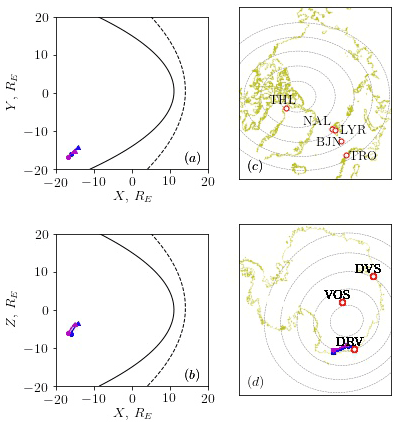
Figure 1The left column shows Cluster 1 and 3 satellite orbits in GSE coordinates (XY – panel a, XZ – panel b), and the right column shows their projection on the map with observatories located in the (c) Northern and (d) Southern hemispheres (12:00–18:00 UT). The initial point and final point are marked with a circle and a triangle respectively.
IMAGE is a European magnetometer network equipped with three-component fluxgate magnetometers with a 10 s initial time resolution (Tanskanen, 2009). The chain is located approximately along the magnetic meridian 100 (MM100), and it covers corrected geomagnetic (CGM) latitudes from Φ=77 to 40∘. Information on the stations utilised in this study and their coordinates is presented in Table 1.
The EISCAT Svalbard radar (ESR) is co-located with the LYR magnetometer station (Φ=75.4∘) and can make detailed measurements of ionospheric electron density, electron temperature, ion temperature, and ion line-of-sight velocity. The radar operates in the 500 MHz band with a peak transmitter power of 1000 kW. In the present paper, data from the 42 m dish (field-aligned pointing position) taken during the International Polar Year (2007–2008) are used.
To map the magnetic field variations from the magnetotail to the ground, data from the Cluster satellite fluxgate magnetometer have been included (Balogh et al., 1997). The values of footprint coordinates are taken from https://sscweb.gsfc.nasa.gov/cgi-bin/Locator.cgi, last access: 2 August 2021. The Tsyganenko 89c model is used for field-line tracing
On 8 August 2007 (day 220), all four Cluster satellites were located in the southern tail lobe at radial distances of between 15 and 20 RE. Specifically, fluxgate magnetometer data from Cluster 1 and 3 are used (which had a separation distance of approximately 1 RE along the Sun–Earth line). Using the TS01 model, Cluster 3 was nearly conjugated with the DRV station (its southern footprint at 17:10 UT was at geographic coordinates of −68.7, 141.4∘ and CGM coordinates of −76, 236∘).
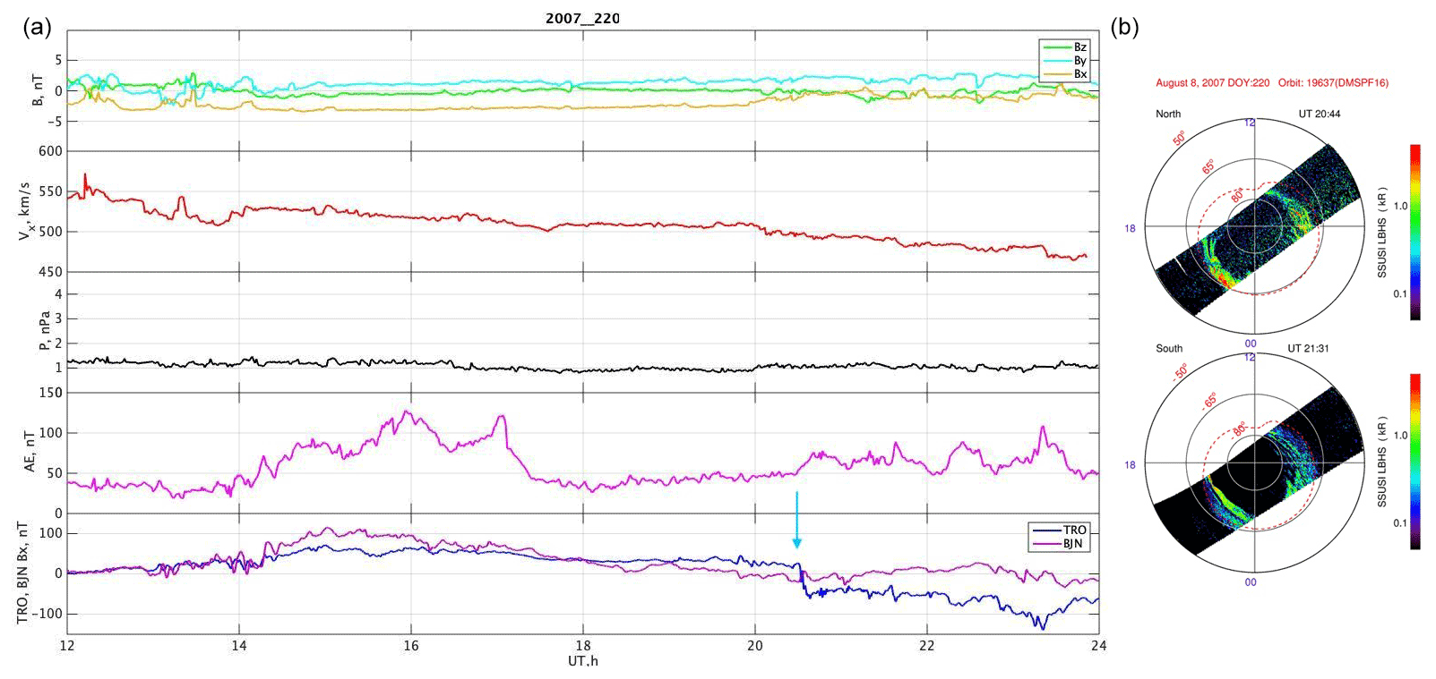
Figure 2Panel (b) presents the particle precipitation seen from the DMSP satellite data. Panel (a) shows the solar wind parameter and ground-based magnetometer data including, from top to bottom, all IMF components, SW speed, SW pressure, the AE index, and the magnetic field data from the TRO and BJN stations. A small substorm is marked using the vertical blue arrow.
2.2 Data processing
Preliminary data processing includes bandpass filtration in the frequency band from 0.8 to 8.3 mHz and decimation to a common 1 min temporal resolution. The lower frequency of the filter window corresponds to an approximate 20 min period. An example of spectra of a non-filtered signal can be found in the Figure S1 in the Supplement. All spectral maxima at frequencies above 1.1 mHz are separated from the filter-related maxima in all spectra shown as examples and used in statistical analysis.
In the case of the magnetospheric satellite measurements of the magnetic field, a local field-aligned system is used. For each time instant, there are two magnetic field vectors in the GSE (Geocentric Solar Ecliptic System) coordinate system (i.e. the instantaneous vector B and the vector averaged over the time window, Bav). The field-aligned component B|| is defined as a projection of B to Bav. The radial component Bρ is normal to Bav, lies in the plane containing B and the Earth centre, and is directed downward. The azimuthal component Bφ is normal to both B|| and Bρ: its direction is determined from the condition that three components form a right-hand triangle. Electron concentrations registered by the EISCAT radar are preliminarily sliced with height, averaged, and passed through the low-band filter with a cut-off frequency of fc=8.3 mHz. On the day of the case study, 8 August, Svalbard was experiencing the midnight Sun period, so the level of background incident solar radiation in the ionosphere was high. Nevertheless, variations in the electron density (ΔNe) are suitable for analysis.
The processing of all (ground- and space-based) data to a common temporal resolution allows a cross-spectral analysis to be performed between the various data sets. The Blackman–Tukey method (Jenkins, 1969; Kay, 1988) is applied to obtain a power spectral density (PSD) for each variable, along with the PSD ratio (R), the spectral coherence (γ2), and the phase difference (Δφ) for each pair of variables. The spectra are calculated in a 96-point (5760 s) sliding window with an 8 min shift between subsequent intervals. Whilst the Blackman–Tukey method has a more course frequency resolution than other similar methods (such as the maximum entropy method), it estimates the PSD with a dispersion that decreases with spectral smoothing.
The spectral estimation parameters were chosen as a compromise between two opposite requirements, namely a better frequency resolution and a lower dispersion of the spectral estimation. One should keep in mind that the dispersion of spectral coherence and phase difference depends on the absolute value of coherence and goes to zero at γ2→1.
OMNI data (time delayed to the bow shock) are used for spectral estimations in the IMF, whereas Cluster data are used for the magnetotail. Various studies have looked at the response time of the magnetosphere to changes in the solar wind (primarily to changes in the IMF). Wing et al. (2002) found a nightside response time to changes in the IMF of ∼ 12 min (at geosynchronous orbit). Given that this study is looking at pulsations with a periodicity of ∼ 12 min (1.5 mHz) and using a 1.5 h sampling window for PSD and coherence estimates, no addition time shift was applied to the OMNI data when evaluating the coherence between them and the Cluster data.
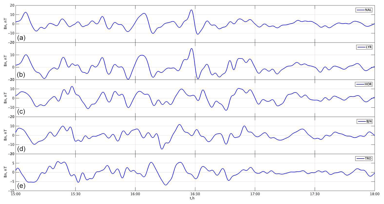
Figure 3A latitudinal profile of geomagnetic pulsations registered on Svalbard (a–d) and in Tromsø (e).
3.1 Space weather conditions and ground-based magnetometer data on day 220 in 2007
The magnetic field data from the TRO and BJN stations, the AE index (auroral electrojet index), and the IMF and SW parameters are shown in Fig. 2a. The figure shows that the IMF was undisturbed, and the absolute value of the BZ component hardly exceeded 3 nT. The absolute value of the solar wind speed (V) was slightly decreasing for the entire period, and the mean value was about 500 km s−1, which corresponds to a moderate SW. The SW dynamic pressure stayed low, and there were no rapid changes. The AE index was increasing from 14:00 to 16:00 UT, and there were two enhancements – at around 17:00 UT and at 20:30 UT. The second enhancement, at 20:30 UT, marked using the vertical blue arrow in Fig. 2a, corresponds to a substorm. Although the magnitude of the substorm bay is small (∼ 100 nT), observations from the DMSP satellite (F16, Fig. 2b, top panel) indicate auroral enhancements consistent with a substorm (i.e. particle precipitation occurring from the magnetotail). It should be added that there are no ground-based optical observations available in the high-latitude northern region due to 24 h daylight conditions in northern Scandinavia.
3.2 ULF fluctuations on the ground and in space
In this section, the analysis of ULF fluctuations in interplanetary space, the magnetotail, and on the ground are presented. The parameters of the IMF/SW fluctuations and geomagnetic pulsations in the magnetotail are calculated throughout the day to illustrate how the parameters of the pulsations in the magnetotail and on the ground are controlled by extra-magnetospheric parameters and the changing (i.e. moving from the auroral oval to the polar cap) of the magnetospheric projection of ground stations. Such a timescale is used in Figs. 4a, 6, 8, and 10. For a more precise analysis of the pulsation spectral properties, a shorter time interval is used in Figs. 4b, c, 11, 12, and 14.
3.2.1 Geomagnetic pulsations on the ground: Northern Hemisphere
ULF pulsations are observed at the ground magnetometer data stations located on Svalbard (from NAL to HOR) and at BJN, and they become indistinct at TRO station, which is situated on the mainland (Fig. 3). For the ground stations, the terms BN and BE are used for the components oriented northward along the magnetic meridian and eastward (orthogonal components) respectively. The time series starts at 15:00 UT and stretches for 180 min. The maximal amplitude reaches ∼ 25 nT from peak to peak at ∼ 16:30 UT for LYR and NAL, and it then decreases to the value of a few nanotesla.
The diurnal variations in the Pi3 (1–4 mHz) power at NAL are controlled by two active regions: the polar cusp, which is responsible for near-noon activity, and the polar boundary of the auroral oval in the morning and evening magnetic local time (MLT) sectors (see Yagova et al., 2004, for details). The station crosses both zones at different universal times (UTs) with a dependence on season and geomagnetic activity in the morning and afternoon MLT sectors. The PSD variation during the day analysed is shown in Fig. 4a. Each data point along the time axis in Fig. 4b corresponds to the starting point of a nearly 1.5 h (96 min) interval. After the cusp-related maximum near MLT noon (09:00 UT), indicated by the vertical red arrow, the PSD reaches a maximum at 13:00 UT (16:00 MLT), indicated by the vertical purple arrow. Afternoon Pi3s, seen after 15:00 UT, do not relate to the cusp activity and are the object of our special interest.

Figure 4(a) Diurnal variations in the spectral power in the 1.2–1.9 mHz frequency band for the NAL bN component, (b) the PSD spectral ratio (R), and (c) spectral coherence (γ2) for the NAL–THL and NAL–HOR station pairs. Near-noon and afternoon maxima are marked using arrows.
To clarify how the contribution of polar cap and auroral oval activity to the NAL pulsations changes with time, the variations in the Pi3 PSD ratio (R) and spectral coherence (γ2) for the THL–NAL and HOR–NAL station pairs are given in Fig. 4b and c. HOR is located ∼ 3∘ southward of NAL on the MM100 chain, whereas THL lies at Φ=84.84∘ (i.e. deep in the polar cap). Although THL is shifted by 5.5 h in MLT from the MM110 stations, the diurnal variation is almost negligible for this location (Yagova et al., 2010), and this station can be taken as an indicator of the conditions in the polar cap. As has been shown (Yagova et al., 2017), the main pulsation power is concentrated in the frequency band from 1.25 to 1.9 mHz and from 08:00 to 20:00 UT (i.e. from pre-noon to almost midnight in MLT). It is seen from the Fig. 4b that both the THL NAL and HOR NAL PSD ratios are less than 1 for near-noon hours (i.e. NAL is dominating), which is probably due to cusp-related activity. From 11:00 to 16:30 UT, the THL NAL spectral ratio is greater than 1, whereas the HOR NAL spectral ratio is approximately 1 (i.e. the PSD deep in the polar cap is maximal). The HOR NAL PSD ratio then grows, while the THL–NAL PSD ratio remains at ∼ 1. From 13:00 to 17:00 UT, the pulsations are coherent for both the THL–NAL and HOR–NAL station pairs, with coherence maxima at 14:00 and 16:00 UT (Fig. 4c). For the first maximum, the HOR–NAL spectral coherence is higher, whereas the coherence for the THL–NAL station pair exceeds that for HOR–NAL for the second maximum. This means that the polar cap (THL) pulsations demonstrate both the highest PSD and coherence with those at NAL after 15:00 UT. This effect can be associated with NAL moving from the auroral oval to the polar cap or can result from temporal variations in the pulsation parameters, such as PSD distributions along a meridian and/or spectral coherence.
An example of the BN component variations and their spectral parameters are presented in Fig. 5. Figure 5a shows a time series of the BN component from 15:44 to 17:20 UT from the NAL, THL, and HOR stations. The pulsation has a period of approximately 11 min (∼ 1.5 mHz), and the peak-to-peak amplitude is about 25 nT at NAL and THL and approximately ∼ 15 nT at HOR. Note that the lower frequency of the filter, fL=0.8 mHz, corresponds to an approximate 20 min period, which is almost 2 times longer than the main pulsation's period. Figure 5b–d show the PSD in each location (panel b), the inter-station spectral coherence (panel c), and the phase difference (panel d). The main maximum of the PSD at all of the stations is found at f1=1.5 mHz, and the value of the PSD decreases with CGM latitude from THL to HOR (Fig. 5b). This spectral coherence for both the NAL–THL and the NAL–HOR station pairs also demonstrates a maximum at f=f1 (as is shown in Fig. 5c). Note that the spectral coherence between NAL and THL (green line in Fig. 5c, d) is higher than between NAL and HOR (blue line in Fig. 5c, d). The pulsations at NAL and THL are almost in phase in the vicinity of f1, whereas a phase difference of ∼ π exists between NAL and HOR. To summarise, the pulsations in the polar cap are characterised by a clear spectral maximum, and the only difference from typical auroral Pc5s is a lower frequency of the main maximum (f1=1.5 mHz).
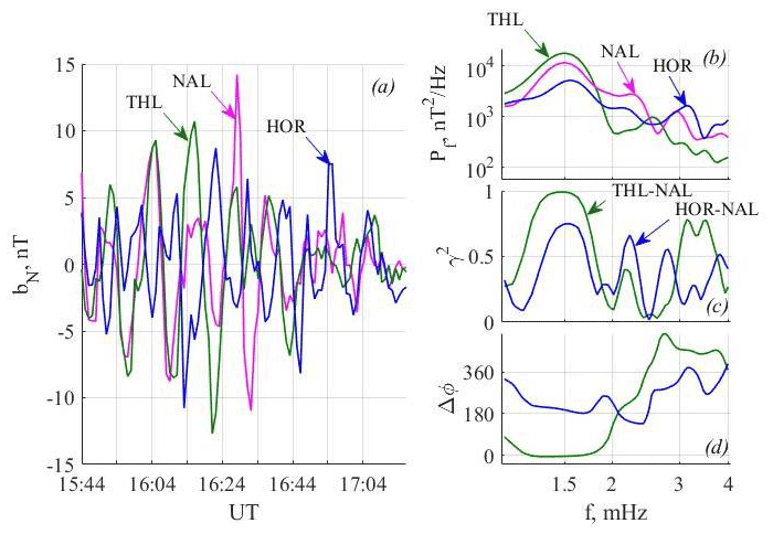
Figure 5(a) Pulsations of the bN component at NAL, THL, and HOR during the interval starting at 15:44 UT; (b) the PSD spectra; (c) the spectral coherence for the THL–NAL and HOR–NAL station pairs; and (d) the phase differences are shown. The THL–NAL and HOR–NAL station pairs in panels (c) and (d) are shown using the same respective colours as THL and HOR in panels (a) and (b).
3.2.2 Magnetic pulsations in the magnetotail and interplanetary space
It is commonly believed that the pulsations in the polar caps are directly driven by fluctuations in the SW. To find a source of the studied pulsations, ULF disturbances in the SW, IMF, magnetotail, and ionosphere were analysed. The average PSD and coherence of magnetic field fluctuations in the IMF, calculated from OMNI, and in the magnetotail, recorded by Cluster 1 and 3, are presented in Fig. 6 (over the same frequency range, 1.2–1.9 mHz, as those presented in Fig. 4). The variations in the PSD of the three IMF components and the field-aligned component b|| in the magnetotail (Cluster3) are given in Fig. 6a. The figure shows that the spectral power in the IMF decreases rapidly at about 13:30 UT (black dot-dashed arrow in Fig. 6a); at ∼ 15:00 UT, a decrease is then seen in the magnetotail (black solid arrow in Fig. 6a). Figure 6b shows the corresponding PSD in the SW dynamic pressure (PSW) and density (n). Whilst there is an increase in spectral power from 10:00 to 15:00 UT, there is a sharp decrease at 15:00 UT (i.e. nearly simultaneously with that of the magnetic field in the magnetotail).
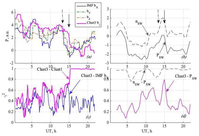
Figure 6The left column shows time variations in (a) spectral power and (c) average spectral coherence for the three IMF components (GSM) and the field-aligned b|| components from Cluster 1 and 3. The right column shows (b) variations in total spectral power and (d) average spectral coherence for the SW density and SW dynamic pressure as well as the field-aligned b|| components from Cluster 3. The dot-dashed arrows indicate the time at which there is a significant decrease in the spectral power in the IMF fluctuations, and the solid arrows indicate the time at which there is a significant decrease in b|| from Cluster 3 and the SW density and pressure.
Simultaneously, the coherence between the pulsations, as measured by Cluster 3 and Cluster 1, in the magnetotail (Fig. 6c) jumps almost to unity, while no severe changes in the Cluster–IMF coherence occur. In the coherence panel (Fig. 6c), only the X component of the IMF is shown, as the coherence variations between the Cluster field-aligned component and the Y and Z IMF components are similar to the Cluster–IMF bX coherence. However, the latter demonstrates a closer agreement with the coherence variations within the magnetotail before the pulsation regime changed at about 15:00 UT (magenta curve in Fig. 6c). A similar decrease is found in the coherence between the magnetic field in the magnetotail and PSW fluctuations (Fig. 6d). As the fluctuations in the SW density and dynamic pressure were almost identical (γ2∼1), only the coherence variations between PSW and Cluster 3 are shown in Fig. 6d.
The change in the pulsation regime in the magnetotail is rather abrupt and can be seen in the time domain as well. Figure 7 shows the pulsations in b|| registered simultaneously by Cluster 1 and 3 and their PSD spectra. The time series for the interval that started at 15:04 UT is given in Fig. 7a. The switch from more or less similar pulsations to almost identical ones is seen at about 15:30 UT and is marked with an arrow. The PSD spectra for the interval that started at 15:44 UT (Fig. 7b) has the main spectral maximum at f=1.5 mHz (i.e. at the same frequency f1 as observed by the ground magnetometers).
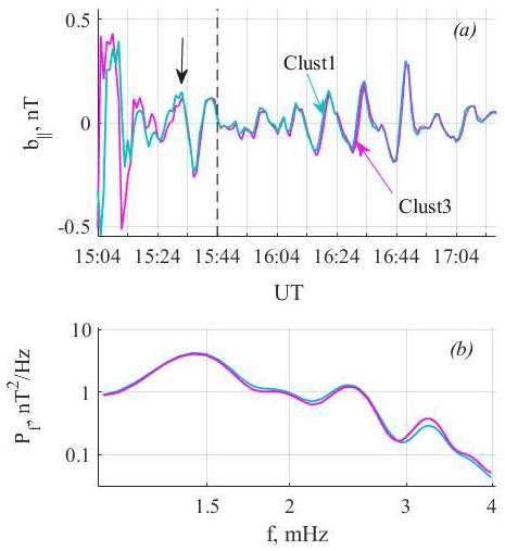
Figure 7(a) Pulsations of the b|| component in the magnetotail, recorded by Cluster 1 and 3 during the interval starting at 15:04 UT. (b) PSD spectra for the 96 min interval starting at 15:44 UT (the start instant of the window for which the spectra are calculated is marked with a vertical dashed line). The change in pulsation regime is marked using an arrow. Pulsations at Cluster 1 and 3 are shown using the same colours in all panels.
To quantitatively describe the variation in the spectral shape of the magnetotail pulsations during the day, we have used the method described by Yagova et al. (2010, 2015). The technique is based upon an expansion of the function σ(F) (a log–log spectrum, where σ and F are the logarithms of the PSD and frequency respectively) into Legendre polynomials, with the resulting first three coefficients (L0, L1, and L2) providing the required quantitative description. In particular, the Q parameter is used (where ), which estimates the deviation of the spectrum from an inverse power approximation (colour noise) near the central frequency of interest.
The results for the Q-parameter analysis, along with the spectral power ratio and phase difference between the different magnetic field components in the magnetotail, as measured by Cluster 3, are shown in Fig. 8. The Q value increases rapidly for all three components (b||, bφ, and bρ) after the PSD in the IMF decreases (i.e. after the millihertz fluctuations in the IMF are switched off; dot-dashed arrow at about 13:30 UT), and it reaches its maximal value at 15:00 UT. It should be noted that the PSD in the SW pressure decreases rapidly at 15:00 UT; however, the Q value for the b|| and bρ magnetic field components in the magnetotail remains high (Q>0.5) until 18:00 UT (and until 17:00 UT for the bφ component). For b||, Q slowly fluctuates between −0.5 and 0.5 from 00:00 to 13:00 UT and afterwards reaches almost 1 within 30 min. The growth for the transversal components (bφ and bρ) after 13:30 UT is not as fast, and Q reaches its maximal value after 15:00 UT.
It has been shown by Pilipenko et al. (2013) that the characteristics of the magnetotail are highly sensitive to the polarisation parameters of the pulsations (in comparison to a simple amplitude-based investigation). The wave polarisation characteristics were changing during the interval analysed, as seen from the variations in the spectral power ratio (R) and phase difference (Δφ) for the b||bρ and the b||bφ component pairs (Fig. 8b, c). For both pairs of components, R exceeds unity almost all day (i.e. the compressional component is dominant). The only exceptions are registered at 03:00, 08:00, and 15:00 UT. In the afternoon MLT sector (i.e. after 09:00 UT), it first increases from 2 to nearly 10 and then drops to 2 for the b||bρ and below unity for the b||bφ component pairs. Between 15:00 and 18:00 UT the average R value is 2–3 times lower than for the previous 3 h. Averaged over the same frequency band, the sinus of the inter-component phase difference, Δφ, is shown in Fig. 8c. Before 15:00 UT, the parameter varies predominantly in the interval [−0.5, 0.8], and it differs for two component pairs. At 15:00 UT it changes to almost unity for both component pairs. This corresponds to a phase difference between the field-aligned and each of the transversal components, indicating a large-scale pulsation with a high fraction of transversal (Alfvén) components. The interval of the phase difference and low R values is seen in Fig. 8 from 15:00 to 18:00 UT (i.e. it coincides with the interval of low amplitude, high Q, and spectral coherence of Pi3 pulsations in the magnetotail).
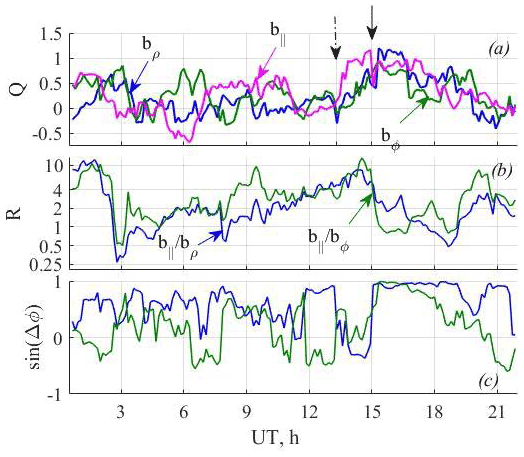
Figure 8Time variations in (a) the parameter Q, (b) the spectral field-aligned to transversal components' spectral power ratio R, and (c) the sinus of phase difference at Cluster 3. The change in pulsation regime in the IMF (at 13:30 UT) and in b|| at Cluster at 15:00 UT is marked by the arrows, similar to Fig. 7.
3.2.3 ULF waves in the magnetotail and on the ground: the inter-hemispheric relationship
As the Cluster satellites were in the southern tail lobe, only a footprint in the southern polar region can be calculated. To understand how the magnetotail pulsations are related to those recorded in the two polar cap ionospheres, the pulsations recorded at Cluster have been compared with those recorded in the southern Polar cap, and pulsations recorded in the southern Polar cap have been compared with those recorded at the northern polar cap. A time series of the pulsations registered simultaneously in the magnetotail at Cluster 3 and in both polar cap ionospheres are presented in Fig. 9a–c, and the spectral coherence for the pairs of components (one ground, one magnetotail) are given in Fig. 9d–f. Pi3s at the DRV station, which is nominally conjugated with Cluster 3 during this time period, have a peak-to-peak amplitude of about 2 nT (Fig. 9a), and the maximal spectral coherence (γ2) at 1.5 mHz (f1) exceeds 0.9 for both field-aligned and transversal components (Fig. 9d). It is the maximal value among all of the satellite–ground pairs. Pulsations at the VOS station, located deep in the southern polar cap, are similar to the pulsations at Cluster 3 and at DRV. Their peak-to-peak amplitudes reach 4 nT (Fig. 9b). The Cluster 3–VOS spectral coherence for both components at VOS and the field-aligned component at Cluster 3 is shown in Fig. 9e. It reaches a spectral coherence of 0.7 at the frequency f1 and is higher than the coherence between the pulsation at VOS and the transversal components at Cluster (not shown here). During this interval, the ground Pi3s are more intensive in the Northern than in the Southern Hemisphere. Hence, the peak-to-peak amplitude at NAL is about 25 nT (Fig. 9c). The maximal coherence, γ2≈0.9, between the NAL and Cluster pulsations is found for the bρ–bN component pair (Fig. 9f). The results show that there is clearly a high coherence between the pulsations observed in the magnetotail and those in the polar cap ionospheres.

Figure 9Pulsations in the magnetotail (Cluster 3) and in bN on Earth. Pulsations at Cluster 3 and at one of the ground stations are shown in panels (a)–(c). The component with the maximal coherence at the f1 frequency with the corresponding station is shown in panels (a)–(c). In panels (a)–(c), the left and right y axes correspond to Cluster 3 and the ground respectively. Spectral coherence for the same satellite–station pairs are given in panels (d)–(f).
A time series of spectral power and coherence, in the 1.2–1.9 mHz frequency band, for different pairs of components for Cluster 3 and VOS is presented in Fig. 10. The VOS station is taken because it is located deep within the polar cap at any local time; thus, the influence of the cusp and auroral activity is minimal. A decrease in spectral power at VOS starts immediately after the “switch off” of IMF fluctuations (this instant is shown using the dot-dashed arrow in Fig. 10). However, the total decrease in spectral power in the ionosphere is not as severe as in the magnetotail. From 15:00 UT (marked by the black solid arrow in Fig. 10), the spectral power measured at VOS remains approximately constant, despite the fact that the spectral power at both Cluster and in the SW dynamic pressure (PSW) (Fig. 6b) has decreased significantly. As a result, the tail to ground (T–G) spectral power ratio (RT−G) during the interval from 15:00 to 18:00 UT is high in comparison with the previous hours (Fig. 10b). The spectral coherence is also higher than its average value during the day, especially for the b|| (Cluster)–bN (VOS) component pair (Fig. 10c).
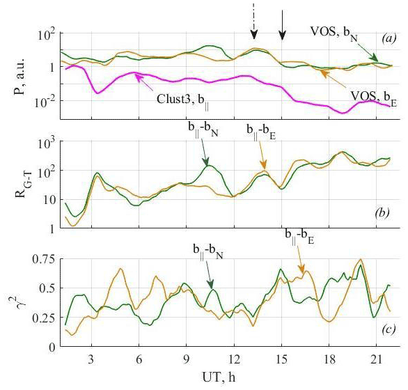
Figure 10Time variations in (a) spectral power, (b) the ground to tail spectral ratio RG−T, and the average (c) spectral coherence in the 1.2–1.9 mHz frequency band for the b|| components at Cluster 3 and both horizontal components at VOS. Time instants with a decrease in the spectral power of IMF fluctuations and pulsations in b|| at Cluster are marked with dot-dashed and solid arrows respectively.
A time series of spectral coherence, in the 1.2–1.9 mHz frequency band, between Cluster 3 and 4 ground-based stations in the both hemispheres is shown in Fig. 11. The DRV station is nominally conjugated to Cluster 3, the NAL station is located in the Northern Hemisphere, and VOS and THL are placed deeper in the southern and northern polar caps respectively, as was mentioned above. The three columns of Fig. 11 correspond to the three magnetic field components in the magnetotail, and the four rows correspond to the four stations. The two g round horizontal magnetic components are colour coded: bN in green and bE in orange. The time interval from 8:00 to 20:00 UT corresponds to hours from local noon to midnight at the TRO station. The highest coherence is found for the bN (DRV)–bφ (Cluster 3) component pair and lasts for 2 h, from 15:00 to 17:00 UT. During the interval, a large-scale pulsation with a high fraction of transversal (Alfvén) components in the spectral power is recorded in the magnetotail. A high (γ2=0.7) but short coherence maximum is also seen in the bN (DRV)–b|| (Cluster 3) component pair. Time evolution similar to bN (DRV)–bφ (Cluster 3) is found for the bE (VOS)–b|| (Cluster 3) and bE (VOS)–bφ (Cluster 3) component pairs, although at somewhat lower absolute values of γ2. As is seen in the bottom two rows of Fig. 11, during the 15:00–17:00 UT time interval, the averaged coherence hardly exceeds 0.5 for all components for Cluster 3–NAL and Cluster 3–THL (i.e. for stations located in the northern polar cap). Generally, the averaged coherence between magnetotail Pi3s and those observed in the northern polar cap is lower than that for the southern polar cap, as is expected, as the Cluster satellites are located in the southern tail lobe.
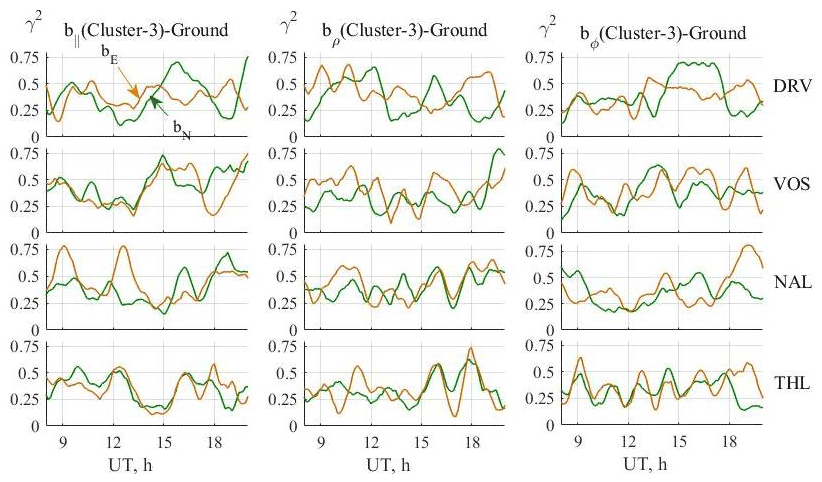
Figure 11Time variations in average spectral coherence in the 1.2–1.9 mHz frequency band for all component pairs formed from Cluster 3 and the four stations. The three columns correspond to the respective b||, bρ, and bφ Cluster components, and the rows show the respective DRV, VOS, NAL, and THL stations. The bN and bE components on Earth are shown in green and orange respectively.
The interrelation between the pulsations in the polar caps and the magnetotail cannot be completely described by their spectral coherences, as the magnetotail data were only available in the southern tail lobe for the studied event. It seems possible to partly compensate for this with the analysis of the coherence between the two polar caps and within each cap. As ionospheric observations are available in the Northern Hemisphere at the NAL longitude (see Table 1), all possible pairs of horizontal components for two combinations of stations (VOS–DVS in the Southern Hemisphere, and DVS–NAL between the two hemispheres) were analysed. It should be noted that the maximal coherence at high latitudes is possible not only for the corresponding components (Lepidi et al., 1996); hence, the maximal coherence for two polar cap stations can be found not between both meridional components but between, for example, the meridional component at the first station and the latitudinal component at the second station. The results for the time interval from 08:00 to 20:00 UT are given in Fig. 12. A high coherence (γ2>0.5) is seen between the bN component at VOS and the bE component at DVS (Fig. 12a) and between the bE component at VOS and both DVS horizontal components for the 15:00–18:00 UT interval (Fig. 12b). Inter-hemispheric coherence over the same time interval reaches a maximum for the bN components of DVS and NAL (Fig. 12c).
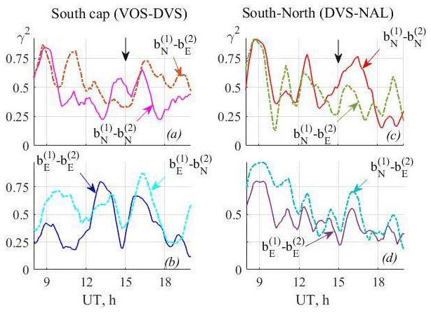
Figure 12Time variations in average spectral coherence in the 1.2–1.9 mHz frequency band between two points in the southern polar cap and between the southern and the northern polar cap stations: (a) bN component at VOS–both horizontal components at DVS; (b) bE component at VOS–both horizontal components at DVS; (c) bN component at DVS–both horizontal components at NAL; (d) bE component at DVS–both horizontal components at NAL. The coherence of the corresponding components (NN and EE) is shown in all panels using solid lines, and the cross-component (NE and EN) coherence is shown using dot-dashed lines. The upper indexes indicate the number of a station in the station pair. The times at which there is a decrease of the spectral power of the pulsations at Cluster are marked with an arrow.
The results of the coherence analysis between the pulsations in the magnetotail and those observed by ground magnetometers in both the northern and southern polar caps show that the Pi3 pulsations recorded after 15:00 UT are characterised by a high coherence in both a space to ground sense and inter-hemispherically. A possible interpretation of this is summarised in the following.
A compressional/shear Alfvén wave in the magnetotail is propagating predominantly in transversal/field-aligned directions respectively. A high coherence between the pulsations observed by ground magnetometers in each polar cap demonstrate that these waves exist in both tail lobes.
This leads to coherent pulsations in both polar caps with a higher coherence between the meridional components for nominally conjugated positions and a higher cross-component coherence for the pulsations inside the southern polar cap.
3.2.4 Electron density fluctuations in the ionosphere
To examine electron density fluctuations in the ionosphere over different altitudes, EISCAT radar data have been used. The background Ne level was high due to solar extreme ultraviolet (EUV) ionisation, but the application of a low-bound filter (see Sect. 2.2) allows the fluctuations of electron density ΔNe for each altitude to be calculated.
A time series of ΔNe, centred in the F region (at h=205 km), along with the bN component of the magnetic field at NAL is shown in Fig. 13a. The spectral power of both time series is shown in Fig. 13b, their spectral coherence is shown in Fig. 13c, and the phase difference is shown in Fig. 13d. The analysis indicates a common spectral maximum at f1=1.5 mHz (Fig. 13b) with a wide coherence maximum with γmax≈0.9 (Fig. 13c). The pulsations are in anti-phase with one another, as is clearly seen from both the time series and the phase difference, which is nearly π at the f1 frequency (Fig. 13d).
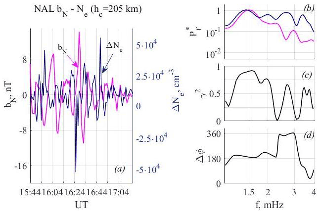
Figure 13(a) Pulsations in the bN component at NAL and fluctuations of Ne in the altitude band from 190 to 220 km during the interval starting at 15:44 UT; (b) the PSD spectra; (c) the spectral coherence; and (d) the phase differences are shown.
Figure 14a shows the temporal variation in the spectral coherence, γ2 (in the frequency band from 1.2 to 1.9 mHz), between ΔNe and the bN component of the magnetic field over an altitude range covering the E and F regions of the ionosphere (from 100 to 450 km). Before 16:30 UT, the highest spectral coherence is registered, with a maximum at about 200 km. The same altitude of maximal coherence is seen from 16:40 to 17:30 UT. Several spots of high coherence were found at lower (∼ 150 km centred at 17:00 UT) and higher (350 km around 16:30 UT and 420 km at 17:00–17:30 UT) altitudes. An altitude profile taken at 15:44 UT is shown in Fig. 14b. Spectral coherence is high (γ2>=0.5) in the altitude range from 120 to 350 km, and the maximal coherence is found at h=205 km. This high coherence between the geomagnetic and Ne pulsations can be a result of modulated particle precipitation. The altitudes where the highest coherence is found correspond to the penetration altitude of electrons with energies in the hundreds of electronvolts (Kozyreva et al., 2007).
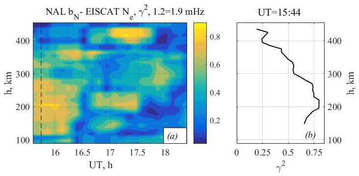
Figure 14(a) Dynamic altitude distribution of spectral coherence between EISCAT Ne and NAL bN in the 1.2–1.9 mHz frequency band during the evening hours, (b) and the altitude distribution of spectral coherence for the 15:44 interval.
Highly coherent pulsations in the Pc5 Pi3 range were observed in the magnetotail and inside the polar caps on 8 August 2007. A spectral analysis of the IMF and SW parameters indicated that the amplitude of pulsations of a similar frequency had decreased significantly by 13:30 and 15:00 UT respectively (Fig. 6). Observations made in the magnetotail (by the Cluster satellites) and in the polar caps (by ground magnetometers and the EISCAT radar) indicate that, at the same time (15:00 UT), the Pc5 Pi3 ULF characteristics in this region changed. A most impressive feature of the pulsations in the magnetotail during the studied hours is a high Q factor, with a central frequency of about 1.5 mHz and extremely high coherence between the two Cluster satellites. The visible pulsations are almost in phase. At the same moment, the contribution of the bρ and bφ (transverse) components to the total spectral power increases. The pulsations are also recorded in both polar caps by ground magnetometers. A coherence analysis shows that the maximal coherence is found for nominally conjugated positions in the magnetotail and in the southern polar cap ionosphere as well as between the two hemispheres for the transversal magnetic field components in the magnetotail and the bN in the ground magnetometer data. For non-conjugated positions in the same hemisphere, the coherence is higher for the field-aligned component in the magnetotail and bE in the ground magnetometer data. This could mean that the wave is a combination of a compressional mode and shear Alfvén modes contributing predominantly to wave transport in the transversal and parallel direction to B respectively. The pulsations also show a high coherence between variations in the electron concentration, ΔNe, and the ground magnetic bN component in the northern polar cap ionosphere. The fact that it is registered in the electron concentration could indicate modulated particle precipitation into the ionosphere from the magnetotail.
These high-quality Pc-like pulsations in the magnetotail probably correspond to some resonance magnetotail mode and started after the external fluctuations had been switched off. Thus, one can speculate that the pulsations in the magnetotail are usually masked by a higher-amplitude broadband ULF “noise” of extra-magnetospheric origin. The existence of quasi-resonance modes at open field lines has been discussed by previous authors for different types of pulsations. Physically, they are related to the reflection of inhomogeneities in the distribution of the Alfvén velocity (e.g. Pilipenko et al., 2005). Moreover, as discussed by Leonovich and Kozlov (2018), the laterally inhomogeneous structure of the nightside magnetosphere can also result in various resonance and waveguide MHD modes in the Pc3–6 frequency range.
It is interesting to note that the studied event perfectly matches with the data set used in Yagova et al. (2017), who showed that the parameter Q is higher for pre-substorm pulsations than for the typical polar cap Pi3s. However, given the current data set, it is not possible to conclusively link this ULF wave event to the substorm observed at 20:30 UT.
Geomagnetic pulsations with a frequency f1∼1.5 mHz were registered on open field lines in both the northern and southern polar caps during quiet, static, space weather conditions on 8 August 2007. These pulsations were also observed in the magnetotail with remarkably high quality and coherence both in space and between the magnetotail and polar cap on Earth. Moreover, the pulsations are seen simultaneously in the ionospheric electron density enhancements in the northern polar cap.
The maximal coherence is found for nominally conjugated positions in the magnetotail and in the southern polar cap ionosphere as well as between the two hemispheres for the transversal magnetic field components in the magnetotail and the meridional (bN) component in the ground magnetometer data. For non-conjugated positions in the same hemisphere, the coherence is higher for the field-aligned component in the magnetotail and latitudinal (bE) component in the ground magnetometer data. This indicates that the wave is a combination of a compressional mode and shear Alfvén modes contributing predominantly to wave transport in the transversal and parallel direction to B respectively.
The ground-based magnetometer data are publicly available from the following sources: IMAGE (https://space.fmi.fi/image/www/, last access: 2 August 2021) and INTERMAGNET (https://www.intermagnet.org., last access: 2 August 2021). Magnetometer data from VOS station are available upon request from http://geophys.aari.ru (last access: 2 August 2021). EISCAT data are publicly available from https://www.eiscat.se/scientist/data/ (last access: 2 August 2021). Cluster and OMNI data are publicly available from CDAWeb (https://cdaweb.gsfc.nasa.gov, last access: 2 August 2021). The maps in Fig. 1 were created using Natural Earth (free vector and raster map data, https://www.naturalearthdata.com, last access: 2 August 2021).
The supplement related to this article is available online at: https://doi.org/10.5194/angeo-40-151-2022-supplement.
NSN suggested the event for the case study and prepared ground-based data for preliminary analysis. NVY developed software and performed data analysis. LJB assisted with EISCAT data analysis, and DAL assisted with DMSP data analysis. DAS provided VOS data. The paper was prepared by NSN and NVY, following discussions with LJB and DAL.
The contact author has declared that neither they nor their co-authors have any competing interests.
Publisher' note: Copernicus Publications remains neutral with regard to jurisdictional claims in published maps and institutional affiliations.
The authors thank Vyacheslav A. Pilipenko for helpful discussions. The authors are also grateful to the institutes that maintain the IMAGE magnetometer array: the Tromsø Geophysical Observatory of UiT, the Arctic University of Norway (Norway); the Finnish Meteorological Institute (Finland); the Institute of Geophysics, Polish Academy of Sciences (Poland); the GFZ – German Research Centre for Geosciences (Germany); the Geological Survey of Sweden (Sweden); the Swedish Institute of Space Physics (Sweden); the Sodankylä Geophysical Observatory of the University of Oulu (Finland); and the Polar Geophysical Institute (Russia). The results presented in this paper rely on data collected at magnetic observatories. The authors acknowledge the national institutes that support these observatories as well as INTERMAGNET for promoting high standards of magnetic observatory practice (https://www.intermagnet.org, last access: 2 August 2021). The authors thank the Arctic and Antarctic Research Institute in Russia for providing ground magnetometer data from VOS station (http://geophys.aari.ru, last access: 2 August 2021). The authors are also grateful to CDAWeb (https://cdaweb.gsfc.nasa.gov, last access: 2 August 2021) for Cluster and OMNI data. EISCAT is an international association supported by research organisations in China (CRIRP), Finland (SA), Japan (NIPR and ISEE), Norway (NFR), Sweden (VR), and the UK (UKRI).
This research was partly funded by the Research Council of Norway (Norges Forskningsråd) within the framework of the PolarProg and INTPART research programmes (grant nos. 246725 and 309135 to Nataliya Sergeevna Nosikova, Lisa Jane Baddeley, and Dag Arne Lorentzen) and by the Russian Foundation for Basic Research (RFBR; grant no. 20-05-00787 A to Nadezda Viktorovna Yagova).
This paper was edited by Minna Palmroth and reviewed by Jonathan Rae and one anonymous referee.
Allan, W. and Wright, A. N.: Magnetotail waveguide: Fast and Alfvén waves in the plasma sheet boundary layer and lobe, J. Geophys. Res., 105, 317–328, https://doi.org/10.1029/1999JA900425, 2000.
Alperovich, L. S. and Fedorov, E. N.: Hydromagnetic Waves in the Magnetosphere and the Ionosphere, Series: Astrophysics and Space Science Library, Springer, the Netherlands, Vol. 353, 2009, XXIV, 418 pp., Hardcover, ISBN 978-1-4020-6636-8, 2007.
Baker, G., Donovan, E. F., and Jackel, B. J.: A comprehensive survey of auroral latitude Pc5 pulsation characteristics, J. Geophys. Res.-Space, 108, 1384, https://doi.org/10.1029/2002JA009801, 2003.
Ballatore, P.: Pc5 micropulsation power at conjugate high-latitude locations, J. Geophys. Res., 108, 1146, https://doi.org/10.1029/2002JA009600, 2003.
Balogh, A., Dunlop, M. W., Cowley, S. W. H., Southwood, D. J., Thomlinson, J. G., Glassmeier, K. H., Musmann, G., Luhr, H., Buchert, S., Acuna, M. H., Fairfield, D. H., Slavin, J. A., Riedler, W., Schwingenschuh, K., and Kivelson, M. G.: The Cluster Magnetic Field Investigation, Space Sci. Rev., 79, 65–91, doi.:10.1023/A:1004970907748, 1997
Bland, E. C. and McDonald, A. J.: High spatial resolution radar observations of ultralow frequency waves in the southern polar cap, J. Geophys. Res.-Space, 121, 4005–4016, https://doi.org/10.1002/2015JA022235, 2016.
Bolshakova, O. V. and Troitskaya, V. A.: Dayside cusp dynamics from the observations of long-period geomagnetic pulsations, Geomagn. Aeron., 17, 1076–1082, 1977.
Borovsky, J. E. and Denton, M. H.: Exploring the cross correlations and autocorrelations of the ULF indices and incorporating the ULF indices into the systems science of the solar wind-driven magnetosphere, J. Geophys. Res.-Space, 119, 4307–4334, https://doi.org/10.1002/2014JA019876, 2014.
De Lauretis, M., Regi, M., Francia, P., Marcucci, M. F., Amata, E., and Pallocchia, G.: Solar wind-driven Pc5 waves observed at a polar cap station and in the near cusp ionosphere, J. Geophys. Res.-Space, 121, 11145–11156, https://doi.org/10.1002/2016JA023477, 2016.
Francia, P., Lanzerotti, L. J., Villante, U., Lepidi, S., and Di Memmo, D.: A statistical analysis of low-frequency magnetic pulsations at cusp and cap latitudes in Antarctica, J. Geophys. Res., 110, A02205, https://doi.org/10.1029/2004JA010680, 2005.
Han, D.-S., Yang, H.-G., Chen, Z.-T., Araki, T., Dunlop, M. W., Nosé, M., Iyemori, T., Li, Q., Gao, Y.-F., and Yumoto, K.: Coupling of perturbations in the solar wind density to global Pi3 pulsations: A case study, J. Geophys. Res., 112, A05217, https://doi.org/10.1029/2006JA011675, 2007.
Heacock, R. and Chao, J.: Type Pi Magnetic field pulsations at very high latitudes and their relation to plasma convection in the magnetosphere, J. Geophys. Res., 85, 1203–1213, https://doi.org/10.1029/JA085iA03p01203, 1980.
Jenkins, G. M. and Watts, D. G.: Spectral analysis and its applications, Holden-Day, San-Francisco, Cambridge, London, Amsterdam, 525 pp., 1968.
Kay, S. M.: Modern spectral estimation: Theory and application, Prentice-Hall, Prentice Hall, New Jersey, USA, 543 pp., 1988.
Keiling, A.: Alfvén Waves and Their Roles in the Dynamics of the Earth's Magnetotail: A Review, Space Sci. Rev., 142, 73–156, https://doi.org/10.1007/s11214-008-9463-8, 2009.
Kepko, L., Spence, H. E., and Singer, H. J.: ULF waves in the solar wind as direct drivers of magnetospheric pulsations, Geophys. Res. Lett., 29, 1197, https://doi.org/10.1029/2001GL014405, 2002.
Kepko, L., Viall, N. M., and Wolfinger, K.: Inherent length scales of periodic mesoscale density structures in the solar wind over two solar cycles, J. Geophys. Res.-Space, 125, e2020JA028037, https://doi.org/10.1029/2020JA028037, 2020.
Kozyreva, O., Pilipenko, V., Engebretson, M. J., Yumoto, K., Watermann, J., and Romanova, N.: In search of a new ULF wave index: Comparison of Pc5 power with dynamics of geostationary relativistic electrons, Planet. Space Sci., 55, 755–769, 2007.
Leonovich, A. S. and Kozlov, D. A.: Kelvin-Helmholtz instability in the geotail low-latitude boundary layer, J. Geophys. Res.-Space, 123, 6548–6561, https://doi.org/10.1029/2018JA025552, 2018.
Lepidi, S., Villante, U., Vellante, M., Palangio, P., and Meloni, A.: High resolution geomagnetic field observations at Terra Nova Bay, Antarctica, Ann. Geophys., 39, 519–528, https://doi.org/10.4401/ag-3987, 1996.
Lyons, L. R., Nagai, T., Blanchard, G. T., Samson, J. C., Yamamoto, T., Mukai, T., Nishida, A., and Kokubun, S.: Association between Geotail plasma flows and auroral poleward boundary intensifications observed by CANOPUS photometers, J. Geophys. Res., 104, 4485–4500, https://doi.org/10.1029/1998JA900140, 1999.
Lyons, L. R., Nishimura, Y., , Kim, H.-J., Donovan, E., Angelopoulos, V., Sofko, G., Nicolls, M., Heinselman, C., Ruohoniemi, J. M., and Nishitani, N.: Possible connection of polar cap flows to pre- and post-substorm onset PBIs and streamers, J. Geophys. Res., 116, A12225, https://doi.org/10.1029/2011JA016850, 2011.
Mann, I. R., Voronkov, I., Dunlop, M., Donovan, E., Yeoman, T. K., Milling, D. K., Wild, J., Kauristie, K., Amm, O., Bale, S. D., Balogh, A., Viljanen, A., and Opgenoorth, H. J.: Coordinated ground-based and Cluster observations of large amplitude global magnetospheric oscillations during a fast solar wind speed interval, Ann. Geophys., 20, 405–426, https://doi.org/10.5194/angeo-20-405-2002, 2002.
Nishimura, Y., Lyons, L. R., Shiokawa, K., Angelopoulos, V. Donovan, E. F., and Mende, S. B.: Substorm onset and expansion phase intensification precursors seen in polar cap patches and arcs, J. Geophys. Res.-Space, 118, 2034–2042, https://doi.org/10.1002/jgra.50279, 2013.
Nishimura, Y., Lyons, L. R., Nicolls, M. J., Hampton, D. L., Michell, R. G., Samara, M., Bristow, W. A., Donovan, E. F., Spanswick, E., Angelopoulos, V., and Mende, S. B.: Coordinated ionospheric observations indicating coupling between preonset flow bursts and waves that lead to substorm onset, J. Geophys. Res.-Space, 119, 3333–3344, https://doi.org/10.1002/2014JA019773, 2014.
Pilipenko, V. A., Mazur, N. G., Federov, E. N., Engebretson, M. J., and Murr, D. L.: Alfven wave reflection in a curvilinear magnetic field and formation of Alfvenic resonators on open field lines, J. Geophys. Res., 110, A10S05, https://doi.org/10.1029/2004JA010755, 2005.
Pilipenko, V. A., Kawano, H., and Mann, I. R.: Hodograph method to estimate the latitudinal profile of the field-line resonance frequency using the data from two ground magnetometers, Earth Planet Sp., 65, 5, https://doi.org/10.5047/eps.2013.02.007, 2013.
Posch, J. L., Engebretson, M. J., Pilipenko, V. A., Hughes, W. J., Russell, C. T., and Lanzerotti, L. J.: Characterizing the long-period ULF response to magnetic storms, J. Geophys. Res., 108, 1029, https://doi.org/10.1029/2002JA009386, A1, 2003.
Rae, I.J., Donovan, E. F., Mann, I. R., Fenrich, F. R., Watt, C. E. J., Milling, D. K., Lester, M., Lavraud, B., Wild, J. A., Singer, H. J., Rème, H., and Balogh, A.: Evolution and characteristics of global Pc5 ULF waves during a high solar wind speed interval, J. Geophys. Res., 110, A1221, https://doi.org/10.1029/2005JA011007, 2005.
Shi, X., Baker, J. B. H.,Ruohoniemi, J. M., Hartinger, M. D., Murphy, K. R., Rodriguez, J. V., Nishimura, Y., McWilliams, K. A., and Angelopoulos V.: Long-lasting poloidal ULF waves observed by multiple satellites and high-latitude SuperDARN radars, J. Geophys. Res.-Space, 123, 8422–8438, https://doi.org/10.1029/2018JA026003, 2018.
Shi, X., Hartinger, M. D., Baker, J. B. H., Ruohoniemi, J. M., Lin, D., Xu, Z., Coyle, S., Kunduri, B. S. R., Kilcommons, L. M., and Willer, A.: Multipoint conjugate observations of dayside ULF waves during an extended period of radial IMF, J. Geophys. Res.-Space, 125, e2020JA028364, https://doi.org/10.1029/2020JA028364, 2020.
Tanskanen, E. I.: A comprehensive high-throughput analysis of substorms observed by IMAGE magnetometer network: Years 1993–2003 examined, J. Geophys. Res., 114, A05204, https://doi.org/10.1029/2008JA013682, 2009.
Troitskaya, V. A. and Guglielmi, A. V.: Geomagnetic pulsations and diagnostics of the magnetosphere, Sov. Phys . Usp., 12 195–218, https://doi.org/10.1070/PU1969v012n02ABEH003933, 1969.
Wang, G. Q., Zhang, T. L., and Volwerk, M.: Statistical study on ultralow-frequency waves in the magnetotail lobe observed by Cluster, J. Geophys. Res.-Space, 121, 5319–5332, https://doi.org/10.1002/2016JA022533, 2016.
Weatherwax, A. T., Rosenberg, T. J., Maclennan, C. G., and Doolittle, J. H.: Substorm precipitation in the polar cap and associated Pc 5 modulation, Geophys. Res. Lett, 24, 579–582, 1997.
Wing, S., Sibeck, D. G., Wiltberger, M., and Singer, H.: Geosynchronous magnetic field temporal response to solar wind and IMF variations, J. Geophys. Res., 107, 1–10, https://doi.org/10.1029/2001JA009156, 2002.
Yagova, N., Pilipenko, V., Rodger, A., Papitashvili, V., and Watermann, J.: Long period ULF activity at the polar cap preceding substorm, in: Proc. 5th International Conference on Substorms, St. Peterburg, Russia, ESA SP-443, 603–606, 2000.
Yagova, N. V., Pilipenko, V. A., Lanzerotti, L. J., Engebretson, M. J., Rodger, A. S., Lepidi, S., and Papitashvili, V. O.: Two-dimensional structure of long-period pulsations at polar latitudes in Antarctica, J. Geophys. Res., 109, A03222, https://doi.org/10.1029/2003JA010166, 2004.
Yagova, N., Pilipenko, V., Watermann, J., and Yumoto, K.: Control of high latitude geomagnetic fluctuations by interplanetary parameters: the role of suprathermal ions, Ann. Geophys., 25, 1037–1047, https://doi.org/10.5194/angeo-25-1037-2007, 2007.
Yagova, N., Nosikova, N., Baddeley, L., Kozyreva, O., Lorentzen, D. A., Pilipenko, V., and Johnsen, M. G.: Non-triggered auroral substorms and long-period (1–4 mHz) geomagnetic and auroral luminosity pulsations in the polar cap, Ann. Geophys., 35, 365–376, https://doi.org/10.5194/angeo-35-365-2017, 2017.
Yagova, N. V.: Spectral Slope of High-Latitude Geomagnetic Disturbances in the Frequency Range 1–5 mHz. Control Parameters Inside and Outside the Magnetosphere, Geomagn. Aeron., 55, 32–40, 2015.
Zhang, S., Tian, A., Shi, Q., Li, H., Degeling, A. W., Rae, I. J., Forsyth, C., Wang, M., Shen, X., Sun, W., Bai, S., Guo, R., Wang, H., Fazakerley, A., Fu, S., and Pu, Z.: Statistical study of ULF waves in the magnetotail by THEMIS observations, Ann. Geophys., 36, 1335–1346, https://doi.org/10.5194/angeo-36-1335-2018, 2018.