the Creative Commons Attribution 4.0 License.
the Creative Commons Attribution 4.0 License.
 | 25 Feb 2021
Lower-thermosphere–ionosphere (LTI) quantities: current status of measuring techniques and models
Minna Palmroth
Maxime Grandin
Theodoros Sarris
Eelco Doornbos
Stelios Tourgaidis
Anita Aikio
Stephan Buchert
Mark A. Clilverd
Iannis Dandouras
Roderick Heelis
Alex Hoffmann
Nickolay Ivchenko
Guram Kervalishvili
David J. Knudsen
Anna Kotova
Han-Li Liu
David M. Malaspina
Günther March
Aurélie Marchaudon
Octav Marghitu
Tomoko Matsuo
Wojciech J. Miloch
Therese Moretto-Jørgensen
Dimitris Mpaloukidis
Nils Olsen
Konstantinos Papadakis
Robert Pfaff
Panagiotis Pirnaris
Christian Siemes
Claudia Stolle
Jonas Suni
Jose van den IJssel
Pekka T. Verronen
Pieter Visser
Masatoshi Yamauchi
The lower-thermosphere–ionosphere (LTI) system consists of the upper atmosphere and the lower part of the ionosphere and as such comprises a complex system coupled to both the atmosphere below and space above. The atmospheric part of the LTI is dominated by laws of continuum fluid dynamics and chemistry, while the ionosphere is a plasma system controlled by electromagnetic forces driven by the magnetosphere, the solar wind, as well as the wind dynamo. The LTI is hence a domain controlled by many different physical processes. However, systematic in situ measurements within this region are severely lacking, although the LTI is located only 80 to 200 km above the surface of our planet. This paper reviews the current state of the art in measuring the LTI, either in situ or by several different remote-sensing methods. We begin by outlining the open questions within the LTI requiring high-quality in situ measurements, before reviewing directly observable parameters and their most important derivatives. The motivation for this review has arisen from the recent retention of the Daedalus mission as one among three competing mission candidates within the European Space Agency (ESA) Earth Explorer 10 Programme. However, this paper intends to cover the LTI parameters such that it can be used as a background scientific reference for any mission targeting in situ observations of the LTI.


The region where the atmosphere meets space, consisting of the mesosphere and the lower thermosphere–ionosphere (LTI), is markedly difficult to measure directly and is therefore sometimes also termed the ignorosphere. The LTI region, spanning from about 80 to 200 km in altitude, exhibits a relatively high atmospheric density, making systematic satellite in situ measurements impossible from circular orbits. This is the region where de-orbiting spacecraft and orbital debris start to burn up while re-entering the atmosphere. Hence sporadic rocket campaigns are currently the main source of in situ observations (e.g, Burrage et al., 1993; Brattli et al., 2009). Remote optical observations require measurable emissions reaching the remote detector; however, there is a significant gap in ultraviolet, infrared, and optical emissions (for Fabry–Perot interferometers) at approximately 100–140 km altitude, allowing only a part of the LTI to be measured remotely. Ground-based radar measurements are also inherently remote but are indispensable especially in characterising the ionised part of the LTI, the ionosphere. Due to the lack of systematic measurements, this region still yields discoveries and surprises; for instance, as recently reported by Palmroth et al. (2020), even citizen scientist pictures of the aurora may be relevant in obtaining new information on the LTI.
A few comprehensive reviews of the LTI have been published in the recent years. Vincent (2015) concentrates on the atmospheric dynamics within the region. Laštovička (2013) and Laštovička et al. (2014) review the trends in the observational state of the art within the upper atmosphere and ionosphere. Sarris (2019) reviews the characterisation status and presents the key open questions especially in terms of measurement gaps within the LTI, while also highlighting the discrepancies between observations and models. A recently accepted review article by Heelis and Maute (2020) describes the challenges within the understanding of the LTI in terms of coupling to the lower atmosphere, the LTI as a source of currents, its coupling to regions above, and the response of the LTI to different drivers. Apart from these recent reviews, one of the most thorough introductions to the LTI dates back to a 1995 book within the American Geophysical Union Geophysical Monograph Series, reviewing, among other aspects, the dynamics of the lower thermosphere (Fuller-Rowell, 2013). These reviews and scientific studies published in the literature explain that the LTI is essentially a transition region with steep gradients in altitude: the dominance of the neutral atmosphere decreases within the LTI as evidenced by the decrease in the neutral density and the drastic increase in the temperature due to absorption of solar extreme ultraviolet (EUV) radiation that occurs within the thermosphere. On the other hand, this is also the region where near-Earth space, controlled by electromagnetic effects, starts to influence the overall dynamics as part of the neutrals are dissociated and the medium has the characteristics of a plasma system. First and foremost, this suggests that the LTI is a region where the underlying physical processes change in nature, warranting understanding both from the atmospheric perspective as well as in terms of space plasma physics.
In the Earth's denser lower atmospheric regions, up to the mesopause around 90 km altitude, the motion of the atmosphere is driven by the solar irradiance and the waves it produces. The dynamics is typically described as a flow governed by the laws of continuum fluid dynamics, for a gaseous fluid that is electrically neutral. In the continuum assumption, averaging is performed over sampling volumes, such that the fluid particles are normally distributed and can thus be described in terms of local bulk macroscopic properties, notably pressure, temperature, density and flow velocity. The continuum assumption requires the sampling volume to be in thermodynamic equilibrium, which implies a high frequency of collisions between atmospheric particles. Atmospheric flow is then predicted by solving the fundamental conservation equations including the conservation of mass, momentum, and energy and a thermodynamic equation of state. The energy from solar irradiance is mostly deposited as sensible and latent heat fluxes and via direct absorption of shortwave (solar) radiative energy, for instance by ozone in the ozone layer and of re-radiated energy, typically by greenhouse gases and clouds.
Above the mesopause, neutral densities become so low that collisions gradually become less important, while the density of the electrically charged ionospheric plasma increases. In contrast to the atmospheric material, near-Earth space plasmas cannot be represented by a similar continuum assumption due to the scarcity of collisions. The laws controlling plasma motion need to be incremented by electromagnetic forces, and thus the forcing from the magnetosphere needs to be taken into account. At high latitudes, the ionosphere is coupled via the magnetic field to the magnetosphere and even further into the solar wind. Further, plasma particles are typically not normally distributed, implying that plasmas cannot be described by e.g. a single temperature. In the transition region between the atmosphere described by the continuum dynamics and geospace described by plasma kinetic theory, at altitudes roughly between 80 and 200 km, the atmosphere starts to be significantly affected by the presence of the ionosphere. The neutral particles and plasmas interact through collisions and charge exchange, which maximise at altitudes between 100 and 200 km but remain important up to around 500 km altitude, the nominal base of the exosphere, beyond which collisions are practically non-existent.
Even though the LTI is characterised as a transition region between the atmosphere and space, it is also markedly a region with characteristics of its own. This is particularly true in terms of the energy sink that the region represents. From the atmospheric perspective, the energy of upward-propagating atmospheric waves, such as planetary waves, tides, and gravity waves (for a review, see Vincent, 2015), is deposited into the LTI. These waves can drive plasma instabilities, which in turn lead to small-scale variations that can cause disruption of radio signals (e.g. Xiong et al., 2016). On the other hand, at polar latitudes, the LTI is a major sink of energy transferred from the solar wind by processes within the magnetosphere and ionosphere, which are not well understood. In particular, during times of very large solar and geomagnetic activity, for example as a response to interplanetary coronal mass ejections (ICMEs, e.g. Richardson and Cane, 2010) and stream interaction regions (SIRs) followed by high-speed streams (HSSs, e.g. Grandin et al., 2019a), this energy input increases substantially and can represent a larger energy source than that provided by solar irradiance. Thus, the energetics, dynamics, and chemistry of the LTI result from a complex interplay of processes with coupling both to the magnetosphere above and to the atmosphere below.
The neutral–plasma interactions and dynamics within the LTI are poorly understood, mainly due to a lack of systematic observations of the key parameters in the region. In the case of scarce observations, the solution is usually to build a model which can be used to obtain information on the region. However, in the case of the LTI, this approach has been markedly difficult due to the complexity of the system: the atmospheric models solving general circulation, chemistry, or the climate system (e.g. Gettelman et al., 2019) normally do not take into account electromagnetic forces. On the other hand, the magnetosphere models using a first-principle plasma approach, either using the magnetohydrodynamics description (MHD; e.g. Janhunen et al., 2012; Glocer et al., 2013) or the (hybrid-)kinetic description (e.g. Omidi et al., 2011; Palmroth et al., 2018), have to be coupled to the ionosphere and neutral atmosphere. The ionospheric first-principle (e.g. Marchaudon and Blelly, 2015; Verronen et al., 2005) or (semi-)empirical models (e.g. Bilitza and Reinisch, 2008) require coupling both to the magnetosphere and to the atmosphere. In the recent years, the different modelling communities have started to integrate the dedicated models towards new regimes; e.g. the Whole Atmosphere Community Climate Model (WACCM) has been extended to cover the thermosphere and ionosphere to about 500 km altitude (WACCM-X Liu et al., 2018a). Likewise, the Whole Atmosphere Model (WAM; e.g. Akmaev et al., 2008) and the Ground to topside model of the Atmosphere and Ionosphere for Aeronomy (GAIA; e.g. Jin et al., 2012) are coupled models of the neutral atmosphere and ionosphere suitable for studying the LTI dynamics. The MHD-based magnetospheric models have been coupled to the ionosphere and neutral atmosphere (Tóth et al., 2005). However, even though the models may currently be the main tool used to provide information on the coupled system, they can only be trusted after careful validation and verification. Hence, ultimately the only way to understand the LTI holistically is by acquiring systematic measurements of the system.
There is a growing recognition that the Earth needs to be studied and understood as a coupled system of its various components. The European Space Agency's (ESA) Living Planet Programme embraces this need, calling for studies of the many linkages within the system. From this viewpoint, it follows that our understanding is only ever as good as the weakest link. One such weak link currently is the connection between the Earth and space. For example, there are considerable changes caused by currents and energetic particles from outer space impinging on the atmosphere, and some of these changes are not well sampled and quantified at all, leading to significant (and maybe even critical) uncertainties. ESA's Earth Explorer 10 candidate mission Daedalus (Sarris et al., 2020) has been designed to explore the LTI systematically for the first time in situ to address the challenges within the LTI described above.
This paper introduces the science behind the Daedalus candidate mission. First, we list the three main outstanding topics under research, related to the LTI energy balance, LTI variability and dynamics, and LTI chemistry. The logic of the paper is to present the outstanding science questions first with a short summarising background. These science topics lead to the need of observing the key LTI parameters, which are divided into those that can be observed directly and those that need to be derived from several other parameters. The bulk of the review concentrates into these direct and derived observables, while the science questions are on purpose concise, giving only a few central literature references. An important choice made in this paper is related to the most important energy deposition mechanism driven by the solar wind and magnetospheric forcing, called Joule heating. This is such a vast topic that it requires a review of its own. However, here the emphasis is on the parameters required to assess Joule heating accurately.
In the two most recent review papers of the LTI, Sarris (2019) emphasises the main gaps in the current understanding of this key atmospheric region and discusses the related roadmaps and statements made by several agencies and other international bodies, whereas Heelis and Maute (2020) provide a detailed review of the physical processes and couplings within the LTI. The purpose of this paper, in turn, is to systematically list and discuss the parameters that can be observed or derived from in situ measurements, underlining the state of the art in observations and numerical models. The intention is to give a background for the measurement setup of any given future mission within the LTI, from the viewpoint of the major outstanding questions. The paper is organised as follows: Sect. 2 presents the outstanding science questions related to the LTI. Sections 3 and 4 review the current understanding of the LTI observed and derived parameters, respectively, which are key to improve the understanding of the region and required to close the outstanding questions. Section 5 ends the paper with concluding remarks.
To assess the role of the LTI as a crucial component within the Earth's atmospheric system, it is important to understand the dominant processes involved in determining the energetics, dynamics, and chemistry of the LTI. Such knowledge is also critical to develop capabilities to specify and forecast space weather phenomena that occur, originate and are modified in this region. This section summarises these broad topics to give the background for the required observed and derived parameters outlined later. Figures 1 and 2 illustrate some of the crucial parameters in terms of energetics (temperatures in Figs. 1a and 2a), dynamics (neutral winds and ion drifts in Figs. 1b–c and 2b), and chemistry (electron density in Fig. 1d, ion/electron and neutral densities in Fig. 2c, and neutral composition in Fig. 2d), both over global scales in Fig. 1 and as altitude profiles near local magnetic midnight during quiet and storm times in Fig. 2. In addition, Fig. 2 recalls the usual nomenclature used in atmospheric and ionospheric studies, indicating the names of the atmospheric layers alongside the temperature profiles (Fig. 2a) and the D, E, and F regions (or layers) in the ionosphere alongside the electron density profiles (Fig. 2c). The LTI is indicated with a grey shading in the profiles, between the mesopause (near 100 km) and 200 km altitude.
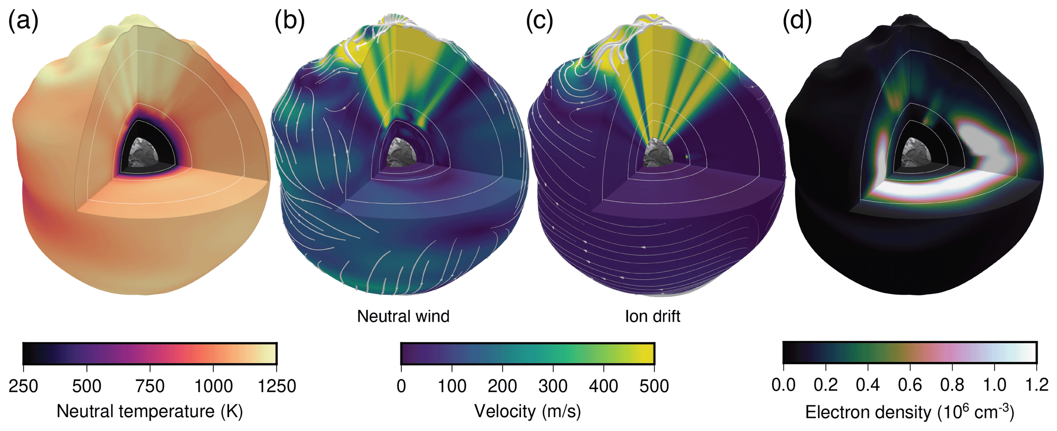
Figure 1Overview of some key atmosphere/ionosphere parameters from the WACCM-X model: (a) neutral temperature, (b) neutral wind magnitude and streamlines, (c) ion drift magnitude and streamlines, and (d) electron density. The model output is from a simulation of the 2015 St. Patrick's Day storm, showing the simulated state of the atmosphere on 17 March 2015, 18:00 UTC, during a period of significant high-latitude energy input. Slices through the model are shown at the top pressure level, at 0 and −90∘ longitude and at −1∘ latitude. The meridional slice over the Greenwich meridian (top right of each sphere) shows a dusk profile, while the 90∘ west slice shows a noon profile. Pressure-level geopotential heights from the model have been exaggerated by 50 times to show vertical detail; concentric circles indicate heights of 100, 200, and 500 km.
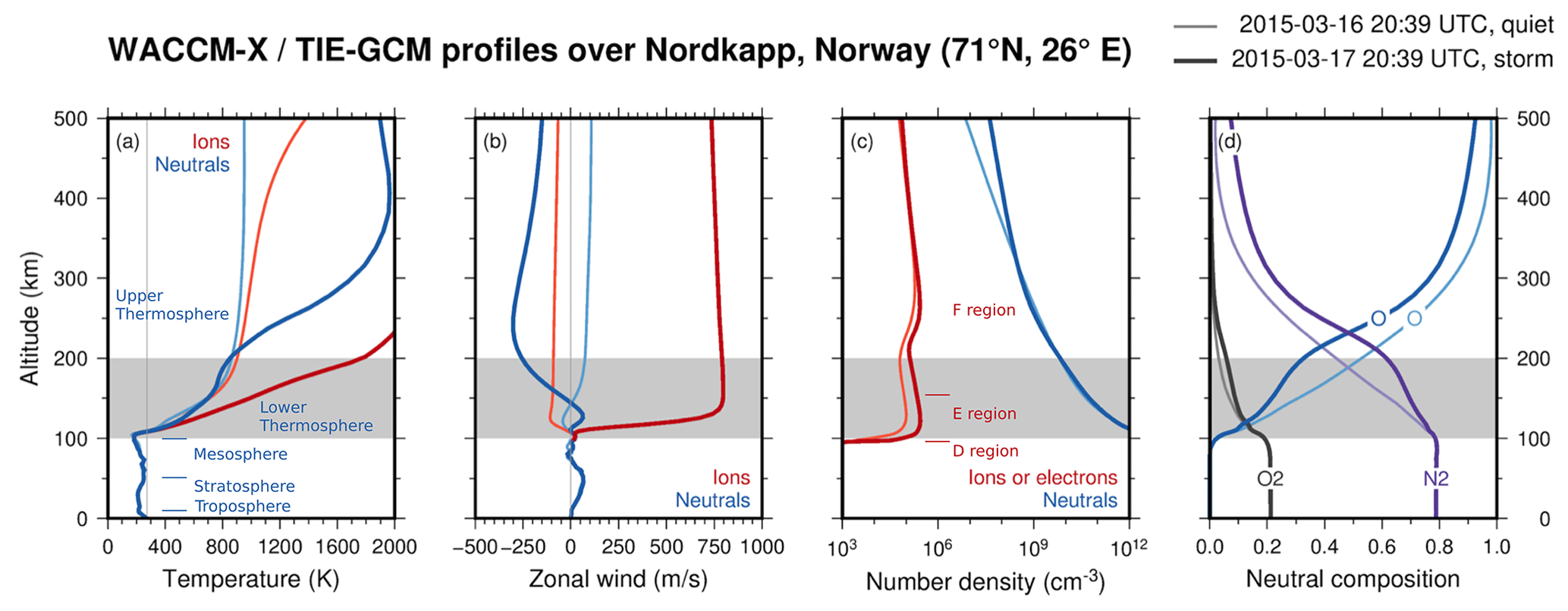
Figure 2Altitude profiles from the WACCM-X and TIE-GCM models of some key atmospheric parameters over Nordkapp (71∘ N, 26∘ E) during quiet time (lighter curves) and during a geomagnetic storm (darker curves) near local magnetic midnight. (a) Neutral (blue) and ion (red/orange) temperature. (b) Zonal neutral wind (blue) and ion drift (red/orange). (c) Neutral (blue) and electron (red/orange) density. (d) Neutral composition (main species). The grey area corresponds to the LTI, between the mesopause and 200 km altitude.
2.1 LTI energetics
In the following, LTI energetics refers to the energy input, deposition, dissipation, and, in general, the energy balance within the LTI. Energetics is driven on the one hand by the solar radiative flux and on the other hand by energy deposition into the LTI from above (near-Earth space) and below (lower atmospheric regions). The solar radiative flux is mostly controlled by the inclination of the planet's rotation axis with respect to the Sun-Earth line, as well as by the distance from the Sun. The energy input from below mainly consists of atmospheric waves propagating upwards. The energy input from above is extracted from the solar wind and processed by the magnetosphere, and it affects, e.g. the motion of the ionospheric charged particles and electromagnetic fields within the LTI (e.g. Palmroth et al., 2004). There are two primary energy sinks which deposit magnetospheric energy into the ionosphere, Joule heating (JH) and particle (electron and proton) precipitation, of which the current understanding suggests that JH represents the larger sink (e.g. Knipp et al., 1998; Lu et al., 1998). However, currently the energy deposited per unit volume at LTI altitudes via JH and particle precipitation is not known. Furthermore, the influence of this energy deposition on the local transport, thermal structure, and composition within LTI altitudes is also poorly known.
2.1.1 Joule heating
Joule heating is in general terms caused by electric currents flowing through a resistive medium, which causes heating within the medium. In the geospace, the current system consists of field-aligned currents (FACs; see Sect. 4.2), which find their closure through ionospheric horizontal currents in the ionosphere (e.g. Sergeev et al., 1996), which is a resistive medium as neutral and charged particles undergo collisions. Ultimately, the power density dissipated by JH is according to Poynting's theorem j⋅E, where j is the electric current density and E the electric field in the frame of the neutral gas. The electric field in the reference frame of the neutral gas, with a neutral gas velocity U≠0, is with B the magnetic field (Kelley, 2009).
In this primary energy deposition mechanism, the additional energy from the magnetosphere forces the plasma to advect relative to the neutral gas, leading to ion–neutral frictional (or Joule) heating. During geomagnetic storms, current knowledge indicates, albeit with large uncertainties, that this energy sink is on a par with the heat created by absorption of solar radiation, which otherwise is the major driver of atmospheric dynamics (Knipp et al., 2005). The effects of moderate to strong geomagnetic activity can be significant at mid and equatorial latitudes, as auroral JH can launch travelling ionospheric disturbances which can have measurable effects down to equatorial latitudes (e.g. Zhou et al., 2016; de Jesus et al., 2016). By enhancing the ion temperature, JH modifies the chemical reaction rates and thus the local chemical equilibrium and ion and neutral composition. The way by which neutral winds, ion drifts and electric fields interplay to generate heating is largely unknown, primarily due to the lack of co-located measurements of all key parameters involved. Since the topic of JH is vast, it is left as a subject of a subsequent paper, while we cover some of the knowledge and open questions of JH in Sect. 4.7.
To understand this energy deposition mechanism, it is imperative to explore the energy deposited into the LTI through JH, by simultaneously measuring the comprehensive set of variables determining JH in the auroral latitudes and 100–200 km altitude regions where it maximises, sampled over a broad range of atmospheric and geomagnetic conditions and at a resolution that captures the key scales associated with this heating process. JH can occur down to very fine scales during active aurora (Matsuo and Richmond, 2008), as in particular electric fields and plasma parameters are believed to have such extremely low scales within the aurora; the relevant scales for JH can be derived via association with the observed scales for auroral structures as obtained by optical measurements and are on the order of ∼ 100 m (e.g. Dahlgren et al., 2016). At the same time, observations indicate that the power (amplitude squared) typically decreases with decreasing wavelengths; thus, to quantify the heating processes, overall it is not necessary to measure electromagnetic fields and plasma parameters down to the smallest scales, which might also be practically difficult. It is therefore considered that a spatial resolution on the order of ∼ 1 km is sufficient for resolving Joule heating on scales that can lead to significant progress in process understanding and quantification as well as in modelling, globally and over long terms. On the other hand, enhanced spatial resolution down to ∼ 100 m, such as could possibly be obtained through sporadic burst-mode capabilities of instruments, would enable the derivation of scale-vs.-power relationship for JH, down to very small scales. One challenge lies in that, since the quantification of JH is significantly affected by the measurements of the Pedersen conductivity (e.g. Palmroth et al., 2005), it is necessary to also characterise how collision cross sections, frequencies, and the resulting conductivities vary with altitude and conditions in the LTI, by simultaneously measuring the comprehensive set of variables determining these parameters over the relevant altitudes and for a range of atmospheric and geomagnetic conditions.
2.1.2 Precipitation-driven energy input
The second most important energy deposition mechanism is caused by particle precipitation, which is typically divided into two categories: lower-energy auroral (∼ 0.01–20 keV, mostly electron) precipitation, depositing energy within ∼ 100–300 km altitude, and energetic (> 30 keV) particle precipitation (EPP), including relativistic (> 1 MeV) energies, consisting of energetic electrons and ions depositing energy below ∼ 90 km altitude (Berger et al., 1970). Auroral ion precipitation occurs, with the specificity of its own that precipitating protons can undergo multiple charge-exchange interactions with atmospheric constituents on their way down, leading to a spreading of the affected area (see the special section by Galand, 2001). The sources of auroral precipitation and EPP are particles both directly coming from the Sun or accelerated by various processes in the magnetosphere. Broadly speaking, auroral precipitation comprises larger number fluxes (Newell et al., 2009), while EPP consists of higher energies. Hence both affect the energy deposition within the LTI, the former through larger areas and the latter through higher energies.
The energy input from particle precipitation is given by the energy of the incoming particles deposited via either dynamical or chemical processes at the altitude of dissipation, for example through electron temperature enhancement, ionisation of neutrals, excitation of neutrals or ions, and dissociation of molecular species producing chemical components (see also Sect. 2.3). The altitude of maximum energy deposition by precipitation is determined by particle energies (e.g. Turunen et al., 2009, Fig. 3): relativistic ions (E>30 MeV) and electrons (E>1 MeV) penetrate down to the stratosphere, energetic ions ( MeV) and electrons ( keV) deposit their energy through ionisation into the mesosphere, while the lower-energy ions (E<1 MeV) and auroral electrons (E<30 keV) impact the thermosphere. The local values of precipitation-induced heating are however largely unknown, as its quantification proves challenging due to the scarcity of suitable observations. Detailed measurements of the energy spectrum and flux of particles passing through the thermosphere as a function of solar/geomagnetic conditions are key to accurately quantifying the impact of precipitation on the climate system (see Sect. 2.3.1).
To quantify the energy deposited into the LTI through particle precipitation, it is necessary to measure the energy spectrum and flux of precipitating particles at the auroral latitudes in regions where it maximises, sampled over a broad range of geomagnetic conditions, and at resolutions in energy and pitch angle that capture the characteristic scales associated with the heating, ionisation, and dissociation processes of interest. Further to the values of energies presented above, which determine the energy range of interest for ion and electron measurements in relation to precipitation-driven energy inputs, since the EPP energy spectra present strong spectral gradients and since spectral features convey information on the precipitating particles' acceleration mechanisms (Newell et al., 2009; Dombeck et al., 2018), high-energy spectra should ideally have at least 128 channels (similar number to the DEMETER/IDP spectrometer; Sauvaud et al., 2006), whilst the spectral energy resolution at low energies should ideally be at least 20 %. Particle precipitation should be measured with a spatial resolution of the order of 10 km or better, based on the corresponding and related typical scales of high-latitude structures such as auroral arcs (Miles et al., 2018). To assess the local response and relative importance of JH and EPP in the LTI, it is necessary to simultaneously measure the comprehensive set of corresponding changes in composition, flows, and temperatures with adequate temporal resolution to capture the involved processes.
2.1.3 Energetics driven by the neutral atmosphere
There are several types of waves within the lower atmosphere which travel vertically towards the LTI and are expected to dissipate there. These waves couple with the neutral wind, temperature field, and density in the LTI. They are also believed to seed plasma instabilities, especially in the low-latitude region, and the upward-propagating waves can produce large shears that may affect the overall circulation within the LTI. In particular, gravity waves (see Sect. 4.9) contribute significantly to the LTI energetics. From a high-resolution WACCM simulation (with horizontal resolution of ∼ 25 km, Liu et al., 2014), it has been calculated that the total upward energy flux by resolved waves at 100 km altitude is 100–150 GW (Liu, 2016), which is comparable to the daily average JH power input (Knipp et al., 2004). This is likely an underestimation of the actual energy flux by gravity waves, since waves with horizontal scales less than 200 km are poorly resolved due to numerical dissipation (or not resolved at all) in the model. Measurements of the related LTI neutral atmosphere parameters (primarily neutral winds, un, neutral temperature, Tn and neutral mass density, ρ) sampled at 10 km resolution would allow detection of small-scale neutral parameter variations as well as gravity waves and tides (e.g. Preusse et al., 2008; Gumbel et al., 2020). The energy deposition rate is also estimated based on parameterised gravity waves: the total wave energy deposition rate at 100 km altitude is 35 GW, and 75 % of that comes from parameterised and resolved gravity waves (Becker, 2017). The role of the neutral atmosphere forcing in LTI energetics can only be estimated, because there are no comprehensive and systematic observations of the coupling between neutrals and ions in the LTI.
2.2 LTI variability and dynamics
This section summarises typical phenomena of spatial and temporal variability in the LTI region and mentions dynamical processes that lead to reorganisation of e.g. neutral or electron density, conductivity, or wind. We consider forcing from above, defined as variations driven by magnetospheric dynamics (Sect. 2.2.1). The current key scientific questions related to LTI variability and dynamics are to understand the ways in which the magnetosphere drives plasma motion in the high-latitude LTI and how this motion affects the motion of the neutrals. We also consider forcing from below through atmospheric waves (Sect. 2.2.2). In this topic, the current key research question is to understand how large shears, sharp gradients, and small-scale plasma instabilities develop in the LTI in response to driving from below. LTI variability and dynamics take a special form at the low geomagnetic latitudes, summarised in Sect. 2.2.3. At low latitudes, the current key scientific question is to quantify the relative contributions of magnetospheric, solar and atmospheric forcing influencing LTI fluid dynamics and electrodynamics.
2.2.1 LTI forcing from above
Magnetospheric driving of the LTI can take the form of electromagnetic driving due to rapid variations in the geomagnetic field and wave–particle interactions within the magnetosphere. Both processes involve the geomagnetic field (Sect. 3.6) and FACs (Sect. 4.2). The geomagnetic field variations are chiefly due to substorms which are often defined as periods of solar wind energy loading and subsequent magnetospheric unloading (e.g. McPherron, 1979). While there is still much debate about the sequence of events that lead to a substorm onset (e.g. Angelopoulos et al., 2008; Lui, 2009), from the phenomenological perspective it is agreed that substorms involve magnetotail reconnection (e.g. Angelopoulos et al., 2008), a FAC system connecting the tail plasma sheet to the ionosphere called substorm current wedge (e.g. Keiling et al., 2009), fast tail plasma flows (e.g. Angelopoulos et al., 1994), dipolarisation of the tail magnetic field (e.g. Runov et al., 2011), plasmoids launched tailwards (e.g. Ieda et al., 2001), and rapidly northward-propagating bright auroral emissions (e.g. Frey et al., 2004). It is not within the scope of this paper to review all the substorm-related subtleties; rather our purpose here is to emphasise the role of substorms as one of the chief magnetospheric drivers of LTI energetics and dynamics. This driving is mostly manifested as increased precipitating particle fluxes as well as intensified FACs.
Another broad category of magnetospheric drivers of the LTI consists of the various waves which modify the proton and electron pitch angles such that the particles precipitate into the LTI. These waves have a multitude of drivers, and their characteristics and role in driving the LTI vary greatly. For example, Alfén waves, driven by solar wind–magnetosphere interactions, propagate into the LTI, transferring energy and momentum as well as modifying LTI local plasma properties such as the density, temperature, and conductance via the total electron content (e.g. Pilipenko et al., 2014; Belakhovsky et al., 2016). Various wave modes, primarily ultra-low-frequency (ULF), very-low-frequency (VLF), and electromagnetic ion cyclotron (EMIC) waves, drive energetic particle precipitation (Thorne, 2010, see also Sect. 3.1), which drives chemistry changes in the LTI (Sect. 2.3). The characteristics and propagation of these waves are important unsolved problems; however, they are well measured only on the ground (e.g. Sciffer and Waters, 2002; Engebretson et al., 2018; Graf et al., 2013; Manninen et al., 2020) or above the LTI around 400 km altitude (e.g. Li and Hudson, 2019). To build a complete picture of wave propagation through the LTI, direct in situ measurements of these waves are required simultaneously with the plasma and neutral gas parameters, which determine the wave propagation in this region. To analyse Alfvén waves and the Poynting flux, both electric and magnetic fields should be simultaneously sampled and at the same cadence. Furthermore, the spectra of measured electric fields should span the entire range of waves that are related to mechanisms important for energy exchange and heating in the lower ionosphere, including two-stream waves, Alfvén waves, ion cyclotron waves, lightning-induced sferics and whistlers, lower hybrid waves, solitary structures, power line radiation and Schumann resonances, as well as various high-frequency (HF) modes. To study wave–particle interactions, the ambient ion cyclotron frequencies and their harmonics should be covered with electric field and density wave measurements. It is noted that, while obtaining the power spectral density of the AC electric field enables the broad characterisation of the variations in the power of these waves, the continuous high sampling of the DC-coupled and AC electric field time series is essential for revealing the detailed waveforms and their non-linear steepening due to heating, as well as their modulation associated with precipitating auroral electrons and their behaviour at the edges of rapidly changing plasma density gradients, structures, and depletions.
Downward LTI forcing is not limited to processes originating from the magnetosphere. Solar flares are also known to enhance electron density and hence JH in the LTI (e.g. Pudovkin and Sergeev, 1977; Sergeev, 1977; Curto et al., 1994; Yamazaki and Maute, 2017). While the solar-flare-driven ionospheric current, or crochet current, near the subsolar region has been intensively studied (e.g. Annadurai et al., 2018), its counterpart at high latitudes has been poorly understood for 40 years, although it significantly enhances pre-existing JH at the auroral electrojets (Pudovkin and Sergeev, 1977). The modification of the auroral electrojets by solar flares can be more than a mere enhancement. Recently, Yamauchi et al. (2020) found that the solar flares can change the direction of the electrojet, and the resulting geomagnetic deviation sometimes exceeds 200 nT. The European Incoherent Scatter (EISCAT) radar observation suggested that even the altitude of JH can be changed for these events. It is quite possible that the altitude of the ionospheric current also changes, but no measurement method to prove this has been proposed.
To understand the forcing from above, it is necessary to explore the momentum transfer between the plasma and the neutral fluid in the LTI, by simultaneously measuring the comprehensive set of variables determining the forces globally, sampling a broad range of atmospheric and geomagnetic conditions, and over timescales that capture the involved processes.
2.2.2 LTI forcing from below
Ionised gas under the influence of the geomagnetic field affects greatly the overall dynamics of the LTI, which makes it distinct, but not decoupled, from the atmosphere. In addition to Joule heating, the electromagnetic coupling asserts the Lorentz force acting on the ionised gas, providing geospace with a lever on the atmosphere and also providing a lever between hemispheres connected by the dipolar geomagnetic field. Furthermore, the electromagnetic forcing affects and is affected by atmospheric variations and disturbances, e.g. by planetary (Rossby) waves, gravity waves, and solar or lunar tides, originating from below the LTI and propagating upwards. Many outstanding issues remain in our understanding of the complex large-scale and global interactions between these processes and forces that act together to determine LTI dynamics. Especially the occurrence of strong flow shears, steep gradients or rapid variations in the LTI parameters have been observed but not been studied systematically due to a lack of consistent measurements of the relevant parameters. Consequently, the effects of such structures on the LTI dynamics are not well known. The physics of the different atmospheric waves is reviewed in Sect. 4.9.
To understand the driving from below, it is necessary to simultaneously measure all the variables defining not only the neutral dynamics, but also the electrodynamics as well as the corresponding local changes in composition, densities, and temperatures at the relevant latitudes and altitudes, sampled over a range of atmospheric and geomagnetic conditions and at temporal scales that capture the key processes involved, including gravity waves, planetary waves, and tides originating from the lower atmosphere. As in Sect. 2.1.3 above, sampling at 10 km resolution would allow the detection of even small-scale variations as well as gravity waves and tides (Preusse et al., 2008; Gumbel et al., 2020).
2.2.3 Variability and dynamics in the low-latitude LTI
At low latitudes, the dynamics of the LTI, comprising the ionosphere E region and lower F region, determines significant parts of the variability of the entire thermosphere and ionosphere through global electric field variations (Scherliess and Fejer, 1999) and related large- to medium-scale plasma transport, the most important phenomenon being known as the equatorial ionisation anomaly (e.g. Walker et al., 1994; Stolle et al., 2008b). The E-region dynamo which results from charged particles transported by thermospheric winds through the nearly horizontal magnetic field (e.g. Heelis, 2004) is understood to play a key role in driving the electric fields and the equatorial electrojet, the latter being a ribbon of strong eastward dayside current flowing along the magnetic equator. While the general principles are described, the significant day-to-day variability of their magnitudes is still the subject of investigation (e.g. Yamazaki and Maute, 2017). A special category of the LTI variability and dynamics within the low latitudes are post-sunset F-region equatorial plasma irregularities, in which the LTI and lower F region are believed to play an important role. Suggested initial perturbations for these plasma irregularities are the variability of the vertical plasma drift at sunset hours (e.g. Huang, 2018; Wu, 2015; Stolle et al., 2008a) and the role of upward-propagating gravity waves (e.g. Krall et al., 2013; Hysell et al., 2014; Yokoyama et al., 2019; Huba and Liu, 2020). The resulting F-region plasma irregularities cause severe effects on trans-ionospheric radio wave signal propagation, leading occasionally to “loss of lock” of space-borne global navigation satellite system (GNSS) receivers (e.g. Xiong et al., 2016, 2020), and are thus an important source of space weather disturbances.
To understand the LTI behaviour within low latitudes, it is imperative to reveal the morphology of flow shears and sharp gradients in the LTI and their role in driving plasma irregularities by simultaneously measuring the comprehensive set of variables that fully describe the LTI, including plasma density at a resolution that captures the relevant processes, sampled over a wide range of latitudes and altitudes. Since the Fresnel scale length that is found to be critical in creating radio wave scintillations, such as on Global Positioning System (GPS) or other kinds of GNSS, is lower than 500 m (Kintner et al., 2007), resolving density structures of less than 500 m, e.g. up to 50 m, covers the pertinent range of scales well.
2.3 LTI chemistry
The chemical composition of the LTI may change in response to particle precipitation (Sect. 2.3.1), temperature increase associated with frictional/Joule heating (Sect. 2.3.2), and through chemical heating (Sect. 2.3.3) resulting from exothermic reactions. The current key science questions in upper atmospheric chemistry are related to the chemical effects of EPP within the mesosphere (and the stratosphere below) as a function of geomagnetic driving conditions. Further, the role of driving conditions from below, including the upward-propagating gravity waves, in influencing the LTI chemistry is not known. Finally, it is not known whether the current model boundary conditions (see below) provide a good representation of the LTI physics as a function of LTI conditions and solar activity. This section is dedicated to summarising the background to these topics.
2.3.1 Precipitation-driven chemistry
Electron and ion precipitation ionise and dissociate neutrals through collisions (Sinnhuber et al., 2012). This has a direct effect in the atmospheric chemical composition via ion chemistry which leads to production of odd hydrogen (HOx) and nitrogen (NOx) (e.g. Codrescu et al., 1997; Seppälä et al., 2015). Considering the LTI coupling to the lower atmosphere, odd nitrogen () is particularly important because it has a long (∼ months) chemical lifetime in polar winter conditions, and it descends to mesospheric and stratospheric altitudes down to ∼ 35 km (Randall, 2007; Funke et al., 2014; Päivärinta et al., 2016) and catalytically destroys ozone (Damiani et al., 2016; Andersson et al., 2018). Ozone is an effective absorber of solar ultraviolet radiation, and its variability modulates the thermal balance of the middle atmosphere and polar vortex dynamics (Brasseur and Solomon, 2005). These perturbations can propagate to surface levels and modulate regional patterns of temperatures and pressures (Gray et al., 2010; Seppälä et al., 2014). Investigation of atmospheric reanalysis datasets and coupled-climate model runs has shown that NOx and HOx have the potential to modify regional winter-time surface temperatures by as much as ±5 K by re-distributing annular mode patterns at mid to high latitudes in both the Northern Hemisphere and Southern Hemisphere (Seppälä et al., 2009; Baumgaertner et al., 2011). To understand these questions, it is necessary to make simultaneous observations of the EPP flux, energy spectral gradients, ion composition, and NOx and measure EPP fluxes with good resolution in the energy and pitch angle. Further, the involved energy spectral gradients need to be described, along with the energy ranges that cover the deposition altitudes from the lower thermosphere to the mesosphere down to the stratopause. These measurements need to be sampled at rates fast enough to resolve different precipitation mechanisms and boundaries on scales of 10 km or smaller. As in Sect. 2.1.2 above, sampling at 10 km resolution would allow the detection of the boundaries of precipitation regions such as auroral arcs (Miles et al., 2018).
The LTI region chemistry is recognised to be important for long-term climate simulations due to its role in solar-driven NOx production and ozone impact (Matthes et al., 2017). However, there are substantial differences between simulated and observed distributions of polar NOx, owing partly to an incomplete representation of electron precipitation (Randall et al., 2015). Further, adequate climate simulations require a NOx upper boundary condition as well as a representation of the dynamical–chemical coupling between thermospheric NOx and stratospheric ozone. For so-called high-top models, with upper boundary in the thermosphere, the boundary conditions can be defined by empirical models based on satellite data (e.g. Marsh et al., 2004), which depend on geomagnetic indices, day of the year, and solar flux. However, current models are based on temporally limited data and do not cover full solar cycles and/or differences between solar cycles, and recent studies indicate a need for improvements (Hendrickx et al., 2018; Kiviranta et al., 2018). To improve the model boundary conditions, it is necessary to make observations of NOx in the polar lower mesosphere below 150 km to characterise the NO reservoir and variability. Preferably, the measurements should be carried out long enough to cover the solar cycle and different EPP events to improve understanding of the drivers for the climate model boundary conditions.
2.3.2 Heating-driven chemistry
Changes in the ion and neutral temperatures, for instance associated with ion–neutral frictional heating, affect the chemical reaction rates in the LTI and can consequently modify the LTI composition. Grandin et al. (2015) found that during high-speed-stream-driven geomagnetic storms the auroral-oval F-region peak electron density can decrease by up to 40 % in the evening magnetic local time (MLT) sector, especially around the equinoxes. The suggested mechanism to account for this electron density decrease is that ion–neutral frictional heating associated with substorm activity may increase the ion and neutral temperatures on timescales much less than an hour, resulting in an enhancement of the electron loss rate by increasing both the chemical reaction rates (functions of the ion temperature) and the molecular densities by upwelling of the neutral atmosphere associated with the neutral temperature increase. A subsequent study by Marchaudon et al. (2018) confirmed that this mechanism, especially through the latter process, can account for the long-lasting F-region peak reduction. Heating-driven composition changes in the LTI have also been revealed in association with subauroral polarisation streams (SAPS; e.g. Wang et al., 2012) and solar proton events (e.g. Roble et al., 1987). However, not many studies discuss heating-driven chemistry in the LTI, indicating a lack of systematic measurements. Composition, density and temperature observations sampled at ∼ 10 km resolution would allow the study of heating-driven chemistry at regional scales (comparable to that studied in Grandin et al., 2015; Marchaudon et al., 2018), as well as the detection of the boundaries of precipitation regions associated with substorms, subauroral polarisation streams, and solar proton events.
2.3.3 LTI chemistry and chemical heating
Chemical heating is one of the main energy sources in the LTI, together with Joule heating, EUV radiation and particle precipitation heating, resulting from the storage in latent chemical form and subsequent release of energy (Beig, 2003; Beig et al., 2008). Chemical heating influences the upper atmosphere in a variety of ways, including the formation of mesospheric inversion layers (Ramesh et al., 2013). Chemical energy is deposited in the LTI through the exothermic reactions typically involving oxygen (atomic and molecular) and ozone (e.g. Singh and Pallamraju, 2018). Neutral species, namely O3, H2O, CO2, OH, and aerosols, are believed to play a role both in the chemistry of the LTI and in the radiative balance of the mesosphere (Mlynczak, 2000). On the other hand, CO2 molecules can induce radiative cooling in the LTI through their emission at 15 µm. Especially between 75 and 110 km altitude, this emission is the only significant cooling mechanism (e.g. Fomichev et al., 1986), while below, radiative cooling by ozone and H2O is also important (e.g. Bi et al., 2011). Quantifying the contribution of chemical heating to the changes in the LTI composition is vital in order to understand the full radiative balance of the upper atmosphere. Furthermore, the spatial and temporal distributions of neutral species could be used as tracers of wave and tidal phenomena (Solomon and Roble, 2015), which affect the overall dynamics of the LTI. Therefore, it is important to obtain measurements of the chemical composition and heating in the LTI. Measuring the neutral temperature and composition at ∼ 10 km resolution would allow the detection of regions experiencing chemical heating. Together with EPP measurements at the same spatial resolution (see Sect. 2.1.2) and numerical models of mesosphere and lower-thermosphere chemistry, this would enable the study of the role of each neutral species in chemical heating and in the radiative balance of this atmospheric region.
3.1 Precipitating particle fluxes and energies
Particle precipitation is very much connected to the overall electrodynamic coupling within the LTI. Precipitation leads to increased ionospheric conductivities (Aksnes et al., 2004) and creates FACs (see Sect. 4.2). FACs close in the E region of the ionosphere, leading to ion–neutral frictional heating (Millward et al., 1999; Redmon et al., 2017, see Sect. 4.7). Since it plays such a leading role in the electrodynamic coupling, we discuss precipitation first.
Particles (electrons and ions) precipitate into the LTI when they are scattered into the bounce loss cone. Pitch-angle scattering can be due to the magnetic field curvature radius being close to the particle gyroradius (Sergeev and Tsyganenko, 1982) or to wave–particle interactions. For instance, lower-band chorus waves, often present in the morningside and dayside magnetosphere, can lead to energetic (E>30 keV) electron precipitation (Thorne et al., 2010), whereas EMIC waves can be efficient in scattering kiloelectronvolt protons and megaelectronvolt electrons into the bounce loss cone (Rodger et al., 2008; Yahnin et al., 2009). Other suggested pitch-angle scattering waves include the plasmaspheric hiss, which may contribute to the precipitation of subrelativistic electrons (He et al., 2018). Phenomena such as pulsating aurora have been found to be associated with precipitating electrons across a wide range of energies (e.g. Grandin et al., 2017b; Tsuchiya et al., 2018), which suggests interaction with whistler chorus waves (Miyoshi et al., 2015) or electrostatic electron cyclotron harmonic waves (Fukizawa et al., 2018). Evaluating the relative contribution of each scattering process to the global precipitation budget is challenging; obtaining particle measurements at multiple pitch angle values in the bounce loss cone with good energy resolution across the energy range could prove decisive in this endeavour.
Precipitating particles can have energies ranging from tens of electronvolt to tens of megaelectronvolt. While low-energy (E≈0.1–30 keV) electrons and protons primarily precipitate at high latitudes, in the polar cusps and in the nightside auroral oval (which is usually above geomagnetic latitude), relativistic electrons from the outer radiation belt (E≈0.1–10 MeV) mostly precipitate at subauroral latitudes, i.e. equatorwards from the auroral oval. Solar energetic particles (E>10 MeV protons), on the other hand, precipitate directly from the solar wind into the polar region (geomagnetic latitudes above ); however, the largest of those events are rare and typically occur only a few times per solar cycle (Neale et al., 2013). Energetic neutral atoms (1–1000 keV, principally within the 100 keV range; Orsini et al., 1994; Roelof, 1997; Goldstein and McComas, 2013) are produced via charge exchange when energetic ions interact with background neutral atoms such as Earth's geocorona. They can play a role in mass and energy transfer to lower latitudes beyond the auroral zone (Fok et al., 2003) and become strongly coupled to precipitating energetic ions in the lower thermosphere (Roelof, 1997).
To date the most comprehensive measurements of particle distributions in the near-Earth environment have been made by flagship spacecraft missions such as DEMETER (Sauvaud et al., 2006), Cluster (Escoubet et al., 2001), Magnetospheric Multiscale (MMS; Burch et al., 2016), Arase (Miyoshi et al., 2018), and the Van Allen Probes (Mauk et al., 2013). However, at high altitudes, bounce loss cone angles have values on the order of a few degrees only, which is too small to be resolved by most particle instruments carried by those spacecraft. On the other hand, at altitudes where low-Earth orbit (LEO) satellites fly, the bounce loss cone at auroral latitudes has its edges at an angle of about 60∘ from the magnetic field direction (Rodger et al., 2010a); it is therefore possible to resolve it with particle detectors. A large number of LEO spacecraft missions have flown particle detectors measuring differential and integral precipitation fluxes. The Solar, Anomalous, and Magnetospheric Particle Explorer (SAMPEX; Baker et al., 1993) mission (1992–2012) produced megaelectronvolt electron precipitation data that have been used in scientific studies (e.g. Blum et al., 2015). The SSJ experiment aboard Defense Meteorological Satellite Program (DMSP) satellites has provided precipitating proton and electron observations in up to 20 channels covering the lower energies (30 eV–30 keV) since 1974 (e.g. Hardy et al., 1984; Redmon et al., 2017); Figure 3a gives an example of differential number flux of precipitating electrons measured by DMSP-F18 on 20 January 2016 in the evening sector of the northern auroral oval. Higher-energy (>30 keV) precipitation observations have on the other hand been routinely provided by NOAA Polar-orbiting Operational Environmental Satellite Space Environment Monitor (POES/SEM) instrument suite since 1979, although measurements have suffered from contamination issues that were corrected by Asikainen and Mursula (2013). Particle detectors can nowadays even be included in nanosatellite missions; one example of upcoming CubeSat missions aimed to measure particle precipitation is FORESAIL-1 (Palmroth et al., 2019), which is expected to measure energetic and relativistic electrons and protons.

Figure 3(a) Auroral electron precipitation differential number flux measured by the DMSP-F18 spacecraft on 20 January 2016 at 18:08:11 UT. (b) Map of diffuse auroral electron energy flux in the Northern Hemisphere given by the OVATION-Prime model at the same time. The radial coordinate is geomagnetic latitude, and the angular coordinate is MLT. The orange star indicates the position of the DMSP-F18 spacecraft.
Indirect observations of particle precipitation can be achieved through various types of observations. Balloon experiments flying in the stratosphere can detect Bremsstrahlung emission produced by precipitating particles interacting with neutrals in the atmosphere, as is done during BARREL campaigns (Woodger et al., 2015). Energetic electron precipitation is routinely monitored from the ground using riometers, which measure the cosmic noise absorption in the D region of the ionosphere associated with particle precipitation (e.g. Hargreaves, 1969; Rodger et al., 2013; Grandin et al., 2017a). Phase and amplitude perturbations to subionospheric man-made narrow-band transmitter signals propagating over long distances are also routinely used to identify energetic electron precipitation (Clilverd et al., 2009). Incoherent scatter radar observations can be used to retrieve precipitating electron energy spectra (Virtanen et al., 2018) and to monitor the ionospheric impact of particle precipitation (Verronen et al., 2015).
Empirical models have been developed by deriving statistical patterns of particle precipitation as a function of geomagnetic activity based on several years of spacecraft observations. The Hardy model (Hardy et al., 1985, 1989) was established by compiling 2 years of DMSP measurements of precipitation and provides differential number fluxes of precipitating electrons and protons as a function of the Kp index. More recently, the OVATION-Prime model (Newell et al., 2014) was developed to predict auroral power as a function of solar wind parameters. This model separates auroral precipitation into four types (diffuse, monoenergetic, broadband and ion); Fig. 3b gives an example of output of the diffuse auroral precipitation, obtained during the conditions when the differential flux shown in Fig. 3a was observed. For higher energies, while the AE-8 (electrons) and AP-8 (protons) maps provide trapped fluxes in the radiation belts (Vette, 1992), the models developed by van de Kamp et al. (2016) and van de Kamp et al. (2018) predict 30–1000 keV electron precipitation fluxes as a function of the Ap index based on analysing energetic electron precipitation observed by POES satellites during 1998–2012. Such climatologies prove particularly useful for space weather predictions and can be used as inputs to ionospheric models, such as the IRAP Plasmasphere-Ionosphere Model (IPIM; Marchaudon and Blelly, 2015) or WACCM (Kinnison et al., 2007). Finally, a few attempts to model particle precipitation in global, first-principle simulations of the near-Earth environment have been made, in magnetohydrodynamics models (e.g. Palmroth et al., 2006a), in some cases coupled with a test-particle code (e.g. Connor et al., 2015), as well as in hybrid-particle-in-cell simulations (e.g. Omidi and Sibeck, 2007) and more recently using a hybrid-Vlasov model (Grandin et al., 2019b, 2020).
3.2 Temperatures
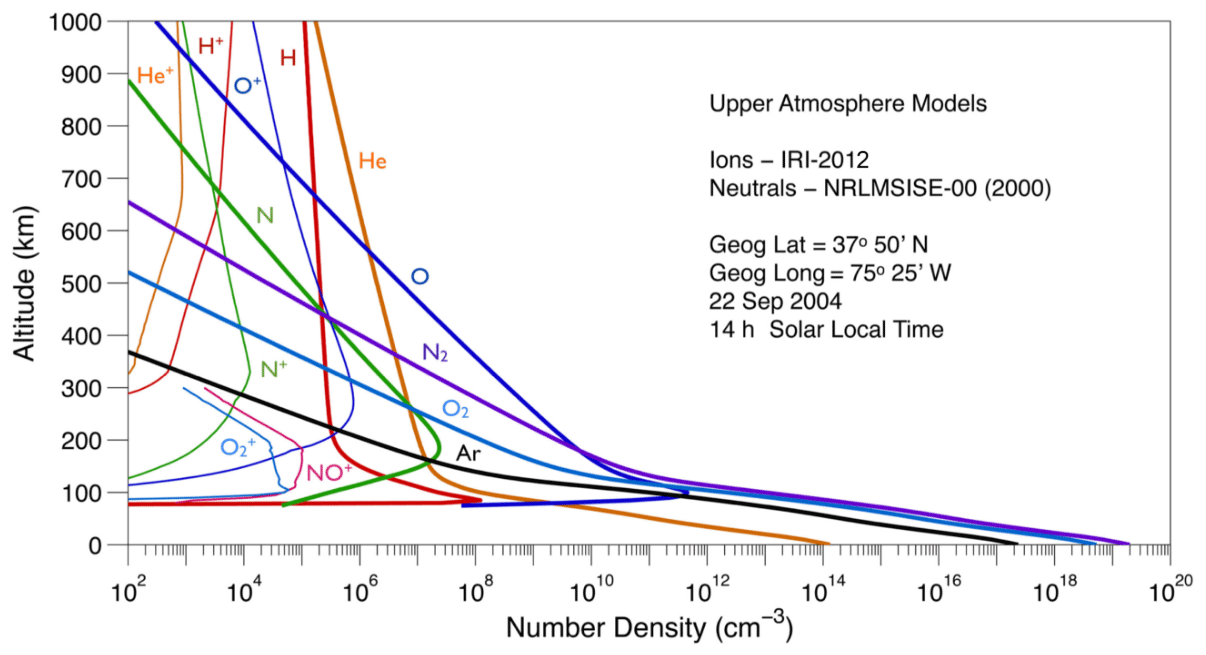
The LTI temperature is a key background parameter, not only because it is a state parameter for the thermosphere itself, but it is also key in ultimately driving neutral winds and atmospheric expansion, as well as determining conditions for chemical reactions. While ion and electron temperatures, Ti and Te, can exceed the neutral temperature Tn by thousands of Kelvin (see Fig. 2a showing neutral and electron temperature profiles at selected latitudes obtained from a WACCM-X simulation), the largest thermal energy reservoir in the LTI is in the neutral gas simply because of the low degree of ionisation in the LTI (see Fig. 4). The largest heat production is by absorption of solar EUV and UV radiation which is ionising and dissociating molecules. This process accounts for the well-known basic vertical structure of Tn and the thermospheric chemical composition.
Reliable measurements of Tn have been difficult and less abundant compared to those of the neutral density itself where especially the analysis of drag on satellite orbits has boosted the available data in the recent decades. In diffusive equilibrium (for each gas component) the profiles of density and Tn are not independent. Early models of the thermosphere were based on this assumption and an empirical formula, sometimes called the Bates profile:
with T∞ the exospheric temperature, the temperature at the base, z0 the height of the base, and H a scale height (Bates, 1959). Sources of Tn measurements include mass spectrometers on sounding rockets, which naturally are relatively sparse, on satellites, which do not cover the lower parts of the LTI well, and by optical methods like UV occultations observed in space and ground-based Fabry–Perot interferometers (FPIs).
Incoherent scatter radars (ISRs) can reliably measure Ti when the mean ion mass is known or assumed. ISR measurements of Ti are a core resource for the construction of empirical models, particularly the widely used NRLMSIS-00 (Picone et al., 2002). Below about 160 km altitude, the molecular ions O, NO+, and N with very similar masses are dominant, and in the topside ionosphere the main ion is O+. In these altitude regions, the Ti estimation by ISR is based on relatively reliable knowledge of the mean ion mass. During geomagnetically quiet times, after sunset, before sunrise, and preferably at mid and low latitudes, ion–neutral frictional heating is not expected to be significant. During geomagnetic activity, ion–neutral frictional (Joule) heating (see Sect. 4.7), particle precipitation (see Sect. 3.1), and magnetic forcing (j×B; see Sect. 4.1) increase, leading to atmospheric expansion and satellite drag (e.g. Liu and Lühr, 2005) and a general upwelling of the thermosphere. While diffusive equilibrium certainly cannot be assumed for a quantitative analysis in such dynamic situations, the upwelling must still be supported by substantial increases in Tn, as simulations have confirmed (Lei et al., 2010).
The thermospheric temperature can be increased significantly during large geomagnetic storms. In numerical simulations of a major storm (8–10 November 2004), Tn was shown to increase from 750 K to up to about 1200 K at high latitudes, whereas at the Equator the increase in Tn over the quiet-time value, ≈1000 K at 400 km height, never exceeded 30 % and was about 15 % on average over the duration of the storm (Lei et al., 2010). The results and observations imply that the energy input into the thermosphere during this geomagnetic storm was invested for one part into geopotential energy, for another part into strong winds reaching a good fraction of the thermal velocity, and for a third part directly into heating of the neutral gas. Both the potential and kinetic wind energy are eventually converted into heat, the latter by molecular viscosity which is important for the dynamics of the thermosphere. The relative contribution of each of these energy sinks during a strong geomagnetic storm requires further investigations to be determined in a quantitative way.
Compared to the solar-cycle-induced variation of Tn, the storm-induced changes seem to be still somewhat smaller. Typically T∞ varies between 750 and 1350 K over a solar cycle, with the power by solar EUV getting converted into both geopotential energy of the atmosphere and directly into heat. The transition between solar-EUV-heated and dark regions is relatively smooth compared to the horizontal temperature gradients that are created by strong, localised Joule and particle precipitation heating. Therefore, the latter probably also generate substantial “available potential energy” in the sense of Lorenz (1955).
3.3 Neutral and ion composition and densities
3.3.1 Neutral and ion composition
The LTI is the region where the neutral atmosphere and the ionosphere are strongly coupled, and the exchange between neutrals and ions is continuous. This exchange occurs through ionisation and recombination and is modulated by the solar UV flux, particle precipitation, and the electrojets. The neutral and ion constituents have however very different scale heights and responses to the drivers such as electrodynamic energy input, electric field, solar UV, or atmospheric forcing (Schunk and Nagy, 1980). Figure 4 provides an example of density as a function of altitude for each of the major neutral and ion species in the terrestrial upper atmosphere, for a given position and time. The ion densities are from the International Reference Ionosphere (IRI) model (Bilitza et al., 2014, 2017) and the neutral densities from the NRLMSISE-00 atmosphere model (Picone et al., 2002). It can be noted that, for a given element, the atomic and ion species can have very different scale heights (e.g. O and O+ or N and N+). This is due to charge-exchange reactions and other aeronomic processes taking place in the upper atmosphere, illustrating the role of chemistry in shaping the atmospheric density profiles.
Composition observations are based on measuring the density of each species, ion or neutral, separately. The in situ composition measurements are performed by ion and neutral mass spectrometers, most notably onboard the Atmosphere Explorer B and C (AE-B and AE-C) spacecraft (1966–1985, PI: H. C. Brinton) and onboard Dynamics Explorer-2 (1981–1983; Hoffman, 1980). These spacecraft had perigees in the 300–400 km range. A few measurements have also been obtained onboard sounding rockets (Grebowsky and Bilitza, 2000). Ion and neutral mass spectrometry technique has been systematically used also for the study of other planetary upper atmospheres in our solar system (Waite et al., 2004; Balsiger et al., 2007; Wurz et al., 2012; Mahaffy et al., 2015). However, after the Dynamics Explorer-2 (DE-2) mission in 1983 no other successful neutral mass spectrometer measurements have been obtained in the terrestrial thermosphere (Dandouras et al., 2018, 2020; Sarris et al., 2020).
For selected ion or neutral species, densities can be obtained also by remote-sensing optical measurements (e.g. Emmert et al., 2012; Qin and Waldrop, 2016). The NASA GOLD (Global-scale Observations of the Limb and Disk) mission, launched in 2018, consists of a UV imaging spectrograph on a geostationary satellite providing remotely measured densities and temperatures in the Earth's thermosphere for O and N2 (https://gold.cs.ucf.edu/, last access: 22 February 2021). Similarly, the NASA ICON (Ionospheric Connection Explorer) mission, launched in October 2019, includes an EUV and a far ultraviolet imager pointing at the Earth's limb (http://icon.ssl.berkeley.edu/, last access: 22 February 2021).
ISR measurements allow in theory to infer the ion composition in the ionosphere, as the ISR spectra depend on the mean ion mass. However, this proves very difficult in practice (Kofman, 2000), and the ion composition is generally assumed when analysing ISR data. On the other hand, assuming an incorrect ion composition when analysing ISR data can lead to large errors in the retrieved parameters (in particular the ion temperature), which is why in several studies the assumed ion composition was corrected using simulations from numerical models (e.g. Blelly et al., 2010; Pitout et al., 2013). A few studies have also made use of ISR observations to estimate the densities of some major neutral species, such as atomic oxygen and hydrogen (Blelly et al., 1992).
The scarcity of composition measurements at Earth's LTI region is thus replaced, to a certain extent, by numerical upper atmosphere models. The National Center for Atmospheric Research (NCAR) Whole Atmosphere Community Climate Model with thermosphere and ionosphere extension (WACCM-X) simulates the entire atmosphere and thermospheric ionosphere, from the Earth’s surface up to ∼ 700 km altitude, and reproduces thermospheric composition, density, and temperatures in good correspondence to measurements and empirical models (Liu et al., 2018a). Besides WACCM-X, IPIM describes the transport of the multispecies ionospheric plasma from one hemisphere to the other along convecting and corotating magnetic field lines, taking into account source processes at low altitudes such as photoproduction, chemistry, and energisation (Marchaudon and Blelly, 2015). It is particularly suited to the study of the E and F regions. D-region studies require a model taking into account ion and neutral species in the mesosphere as well, including cluster ions and negatively charged ions. The recently developed WACCM-D (Verronen et al., 2016) combines photoionisation by solar ultraviolet and X-ray radiation, ionisation by particle precipitation and galactic cosmic rays, and a detailed chemistry scheme of 307 reactions of 20 positive ions and 21 negative ions. Particularly aimed for particle precipitation studies, WACCM-D allows for simulations of NOx production in the mesosphere and LTI, dynamical connections to the stratosphere, and the impact on ozone (Andersson et al., 2016; Kyrölä et al., 2018; Verronen et al., 2020). The Sodankylä Ion-neutral Chemistry (SIC) model is another D-region photochemical model which has been used in studies of various phenomena in the mesosphere and LTI (e.g. Verronen et al., 2005; Kero et al., 2008; Seppälä et al., 2018).
3.3.2 Neutral and ion densities
Neutral densities can be derived from a number of observation techniques. Tracking the orbital decay due to atmospheric drag of space objects from the ground is one of the first techniques still applied today (Storz et al., 2005; Doornbos et al., 2008; Bruinsma, 2015). While tracking and orbit ephemeris data are available from the 1960s onwards, the effects of drag typically have to be integrated over one or more orbital revolution and often up to several days, in order to derive sufficiently accurate densities. By combining orbit data from multiple tracked objects, long time series on global neutral density changes have been reconstructed at a resolution of up to 3 h with US space surveillance data (Storz et al., 2005), and at 1 d resolution using publicly available data (Emmert et al., 2008). A more accurate observation technique is GNSS tracking of satellites, which can provide a resolution along the orbit of up to 10 min, depending on the tracking accuracy and the altitude. As opposed to tracking techniques, accelerometers provide instantaneous measurements of the non-gravitational acceleration. The first multi-year accelerometer measurements were performed by the Atmospheric Explorer missions and the Castor satellite in the 1970s (Beaussier et al., 1977).
A new era began in the year 2000 with the launch of the Challenging Minisatellite Payload (CHAMP) satellite, which carried a precise three-axis accelerometer, star cameras and a GPS receiver as part of the scientific payload. The combination of the GPS tracking and the accelerometer measurements allowed us to obtain well-calibrated accelerations that could be used to derive accurate neutral density data at a high resolution along the orbit. The same combination of observation techniques is employed by the Gravity Recovery and Climate Experiment (GRACE), Gravity Field and Steady-State Ocean Circulation Explorer (GOCE), Swarm and GRACE-FO satellites, which were launched in 2002, 2009, 2013 and 2018, respectively. All of these satellites have provided a wealth of neutral density observations in the altitude range from 200 to 500 km.
Deriving neutral density from acceleration measurements requires knowledge of the neutral composition of the atmosphere to accurately model the gas–surface interactions that influence the aerodynamic coefficients of the satellites. That knowledge is based on neutral mass spectrometer data collected in the 1960s, 1970s, and 1980s. As indicated in Sect. 3.3.1, since the end of the Dynamics Explorer-2 mission in 1983, no successful neutral mass spectrometer measurements have been obtained. Like accelerometers, neutral mass spectrometers need to be calibrated to transform the precise relative composition measurements into accurate absolute number densities. The derivation of the neutral density and wind from the accelerometer observations, when the accelerometer is located in the centre of mass of the satellite, is based on the measurement of the total linear non-gravitational acceleration by the instrument. For a three-axis accelerometer, the raw accelerometer observation vector aobs typically needs to be calibrated by applying a 3×3 diagonal scale factor matrix S and by adding a bias vector b (Doornbos, 2011):
Typically, accelerometer scale factors are considered to be nearly constant (Tapley et al., 2007), whereas biases are typically estimated on a daily basis. Both the scale factors and biases can be estimated precisely from tracking by the GPS (Helleputte and Visser, 2009). It is anticipated that spaceborne multi-GNSS receivers will make this estimation even more robust and precise.
The calibrated accelerometer observations acal include the aerodynamic accelerations aaero, but also need to be reduced first by removing other contributions:
where asrp, aalb, and aIR represent the accelerations caused by solar radiation pressure, Earth albedo, and Earth infrared radiation, respectively. The remaining accelerations arem are assumed to be negligible. The aerodynamic acceleration is typically modelled as (Doornbos, 2011)
where Ca is a dimensionless force coefficient (Anderson, 2010), Aref represents a reference area, m the satellite mass, ρ the neutral density and vr the velocity of the atmosphere relative to the spacecraft body. This velocity includes the neutral wind. Doornbos (2011) proposed and implemented an iterative scheme for successfully deriving neutral density and wind from accelerometer observations for low-flying satellites such as CHAMP and GOCE.
The neutral density can also be derived by adding the number densities of the individual species composing the neutral atmosphere as measured by a neutral (or neutral and ion) mass spectrometer. This technique has been systematically used for the study of planetary upper atmospheres (Waite et al., 2004; Balsiger et al., 2007; Wurz et al., 2012; Mahaffy et al., 2015). Similarly, the thermal ion density can be derived by adding the number densities of the individual ion species composing the ionosphere (Hoffman et al., 1974; Chappell, 1988; Welling et al., 2015). A low-Earth-orbiting satellite mission comprising well-calibrated instruments such as a GPS receiver, an accelerometer, and a neutral and ion mass spectrometer could allow us for the first time to measure simultaneously neutral and ion densities and compositions to determine the accuracy of the summing method.
3.4 Neutral winds
In the LTI, neutral winds are strongly influenced by many external drivers like geomagnetic and solar activity and tidal, planetary and gravity waves (Rees, 1989). Figures 1b and 2b show the global distribution and selected altitude profiles, respectively, of the neutral winds during the St Patrick Day geomagnetic storm on 17 March 2015, obtained from a WACCM-X simulation. These figures show in particular that large magnitudes of several hundred metres per second can be reached at polar latitudes.
The characterisation of neutral winds across a wide range of altitudes is critical to correctly quantify processes such as Joule heating (e.g. Kosch et al., 2011) or F-region dynamics (e.g. Billett et al., 2020). In the lower altitude range of the LTI, the neutral wind characteristics are poorly known. At higher altitudes, thermospheric neutral winds have been in the last decades retrieved by e.g. accelerometers (Doornbos, 2011) onboard many satellite missions like Dynamics Explorer, CHAMP, GOCE, and Upper Atmosphere Research Satellite embedding a Wind Imaging Interferometer (UARS/WINDII). The accelerometer data can be further processed with a high-fidelity geometry and aerodynamic modelling to obtain thermospheric products (March et al., 2019a, b). The availability of cross-track accelerations has led to a large amount of horizontal cross-wind data (Sutton et al., 2005; Cheng et al., 2008; Doornbos et al., 2010), while the vertical acceleration was generally assumed too small to obtain reliable wind measurements (Visser et al., 2019). Vertical winds are more difficult to retrieve; however, with the help of linear and angular accelerations, this was recently done with the latest release of the GOCE thermospheric data, which are available in the ESA GOCE virtual archive (https://goce-ds.eo.esa.int/oads/access/, last access: 22 February 2021).
Besides in situ measurements by spacecraft, various ground-based instruments enable neutral wind observations by remote sensing. Wide-field FPIs, or scanning Doppler imagers (SDIs), measuring the Doppler shift of the airglow/auroral red (630.0 nm) and/or green (557.7 nm) emission lines allow us to retrieve the F-region and E-region neutral winds. One example of SDI is SCANDI (Aruliah et al., 2010), which observes the red line to measure neutral winds at around 250 km altitude within a large field of view in multiple horizontal bins giving a spatial resolution on the order of 100–300 km, with a time resolution of about 8 min. Narrow-field FPIs use the same principle to observe neutral winds within smaller spatial bins (<10 km) with a high precision in the pointing direction (Shiokawa et al., 2012). The downside of those ground-based optical instruments is that they require clear and dark skies to provide neutral wind measurements. A cross-comparison of SDI and narrow-field FPI measurements can be found in Dhadly et al. (2015). Finally, incoherent scatter radars can also allow us to estimate neutral winds using a method called stochastic inversion (Nygrén et al., 2011). While they provide a lower time resolution and larger uncertainties, on the other hand they allow us to retrieve altitude profiles in the E region (95–135 km altitude in 10 km bins) and are not affected by cloud cover or daylight.
Various empirical models of neutral winds have been built by combining large datasets consisting of observations from satellites, rockets, and ground-based instruments. The prime example of neutral wind climatologies is the Horizontal Wind Model (HWM) series (Drob et al., 2008, 2015). The HWM is constantly under development at the Naval Research Lab, and its latest edition is the HWM-14 (Drob et al., 2015). Neutral winds are also studied using first-principle models, wherein equations describing dynamics, as well as photochemical, transport, electrodynamical, thermodynamical, and radiative processes, are solved self-consistently. Examples of such models include, e.g. the Thermosphere Ionosphere Electrodynamics General Circulation Model (TIE-GCM; Richmond et al., 1992), WACCM (Liu et al., 2010), the Global Ionosphere Thermosphere Model (GITM; Ridley et al., 2006), and the Magnetosphere-Thermosphere-Ionosphere Electrodynamics General Circulation Model (MTIE-GCM; Peymirat et al., 1998).
3.5 Ion drift velocity and electric fields
Ionospheric convection corresponds to the plasma drift relative to the neutral medium, being typically from dayside to nightside through the midnight meridian and back towards the dayside at auroral latitudes. Convection is an important ionospheric parameter which reflects the complex coupling between the solar wind and the magnetosphere as well as internal magnetospheric processes such as reconnection in the magnetotail (Dungey, 1961; Cowley and Lockwood, 1992). The high-latitude flows generally form two cells, with anti-sunward flow over the polar cap and return sunward flows at lower latitudes in the auroral zones, both in the evening and morning sectors. However, both the spatial extent of the flow system and the magnitude of the flows vary and are related to the solar wind parameters, specifically to the north–south (Bz) and east–west (By) components of the interplanetary magnetic field (IMF, e.g. Thomas and Shepherd, 2018).
Ionospheric ion drifts commonly refer to the F region above 200 km, where collisions between ions and neutrals are scarce, and the relationship between the plasma velocity and the electric field E is given by , where the drift speeds of ions vi and of electrons ve are equal since the ion–neutral collisions are very weak, and where B is the Earth's magnetic field and B its magnitude. Therefore, strong plasma flows correspond to strong electric fields. This is illustrated in the global distribution and example profiles of the ion drift speed given in Figs. 1c and 2b, obtained from WACCM-X and TIE-GCM simulations of the St Patrick's Day storm and revealing that ion drifts take place at high latitudes only, where strong electric fields are present.
Because magnetic field lines are equipotentials due to high parallel conductivities, plasma convection is almost perfectly projected from the magnetosphere to the ionosphere (e.g. Weimer et al., 1985; Marchaudon et al., 2004), when taking into account the magnetic field convergence towards the surface, as can be seen in Fig. 2b through the fact that ion drift speeds do not exhibit a significant altitude variability above ∼ 150 km. However, ionospheric convection, or ion drift, displays rapid variations on the order of a few minutes, which directly reflect the variable solar wind–magnetosphere coupling. Ion drift measurements have been developed in the 1970s–1980s with the building of ground-based facilities (HF coherent radars, ionosondes and incoherent scatter radars) and the launch of satellites flying in the ionosphere or at higher altitudes. For clarity, this section is divided into subsections reviewing the different techniques.
3.5.1 HF coherent radars and SuperDARN
HF coherent radars transmit oblique waves and use ionospheric refraction of the signal to reach very large distances from the radar. They generally cover a large field of view (50–60∘) by sounding several successive beams with a high-temporal resolution (1–2 min). A backscattered signal on ionospheric density irregularities aligned with the magnetic field allows retrieval of the Doppler shift of the echoes, giving access to the ion drift at successive distances along the beam (15–45 km resolution) (Greenwald et al., 1985; Villain et al., 1985). The main limitation of this measurement technique is the access to only one component of the ion drift, called line-of-sight velocity. To overcome this, HF radars have been paired such as to have a common volume of sounding where full ion horizontal velocity vectors can be reconstructed.
At the beginning of the 1990s, a network of HF radars called the Super Dual Auroral Radar Network (SuperDARN) was developed and pairs of radars were built first along the auroral zones of the Northern Hemisphere and Southern Hemisphere in order to reconstruct the global convection pattern at high latitudes (Greenwald et al., 1995). However, the often incomplete coverage of measured echoes in the field of view of each radar did not allow good combined measurements coming from pairs of radars. To overcome this problem, statistical maps of convection were first built from one radar, gridded in geomagnetic latitude and MLT and binned with respect to IMF (Ruohoniemi and Greenwald, 1996; Ruohoniemi and Baker, 1998). These maps were then combined with real line-of-sight velocities of each radar to enhance the realistic representation of the ion drift. This method allows a continuity of coverage in each polar hemisphere but is only fully representative in regions where real fitted vectors are reconstructed from radars measurements. More recently, the radar network has been extended in the polar cap and mid-latitude regions (Nishitani et al., 2019), allowing for a better coverage during perturbed periods. New versions of statistical maps have also been proposed using all radars in each hemisphere over a larger time period and with different types of binning to take into account seasonal variations, mid-latitude echoes, IMF variations or directly geomagnetic activity levels (Ruohoniemi and Greenwald, 2005; Pettigrew et al., 2010; Cousins and Shepherd, 2010; Thomas and Shepherd, 2018).
The strength of the SuperDARN radars is their capability to follow large-scale and meso-scale convection with an excellent spatio-temporal resolution, whose patterns are often similar to the statistical maps obtained for equivalent IMF and/or tail conditions (e.g. Provan et al., 1999; Wild et al., 2003; Huang et al., 2000; Senior et al., 2002; Imber et al., 2006). Complete reviews of SuperDARN radars can be found in Chisham et al. (2007) and Nishitani et al. (2019).
3.5.2 Ion drift measurements onboard satellites
Ion drift has also been systematically recorded with satellites, originally through the combination of ion-drift metre (IDM) and retarding potential analyser (RPA) measurements. The IDM measures velocities in the direction perpendicular to the satellite velocity vector; the RPA measures along-track velocities and provides estimates of ion composition and ion temperature as well. The first satellites to make such measurements were AE-C in the 1970s (Hanson et al., 1973) and DE-2 in the 1980s (Heelis et al., 1981). To this day the AE-C measurements remain the only published satellite-based measurements of the LTI below 200 km altitude. The AE-C observations were followed by the series of DMSP satellites, which operate around 800 km altitude on polar orbits with orbital periods spanning from 90 to 120 min. The DMSP spacecraft generally cross the auroral zone and the polar cap region close to the dawn–dusk plane in about 10 to 15 min, which makes a full reconstruction of the instantaneous convection pattern impossible. However, these different satellites have been used to study specific localised phenomena with great success, such as the convection in the polar cusp, cleft, and cap (e.g. Heelis et al., 1976; Heelis, 1984; Burch et al., 1985; Heelis et al., 1986), and the properties of enhanced convection at subauroral latitudes known as subauroral ion drift (SAID) or SAPS (e.g. Spiro et al., 1979; Anderson et al., 1991). Moreover, the DMSP data have successfully been used to build statistics of high-latitude convection patterns with respect to IMF conditions, seasons, and hemispheres, from which well-known models have been derived (e.g. Heelis et al., 1982, Hairston and Heelis, 1990, and Weimer, 2005 with DE-2 data or Rich and Hairston, 1994 and Papitashvili and Rich, 2002 with DMSP data).
The Swarm mission (Friis-Christensen et al., 2008), launched in 2013, consists of three satellites in polar circular orbits at altitudes of ∼ 450–500 km. Swarm incorporated a new method of measuring ion drift and temperature known as thermal ion imaging, or TII (Knudsen et al., 2017). TII sensors produce two-dimensional images of the low-energy ion distribution at rates as high as 125 s−1 and can be used to determine higher-order features of the ion distribution functions such as ion temperature anisotropy (Archer et al., 2015). Lomidze et al. (2019) showed that the Swarm TII cross-track ion velocity measurements are consistent with a DE-2-based convection model (Weimer, 2005). TII measurements from Swarm have revealed the existence of intense flow channels at the boundary of the nightside R1/R2 FAC systems (Archer et al., 2017) and in association with sub-auroral “STEVE” arcs in which the ion flow velocity can exceed 5 km s−1 (MacDonald et al., 2018). Swarm ion flow measurements have been used in conjunction with magnetic field measurements in a number of studies of low-frequency electrodynamics including measurements of quasi-static Poynting flux (see Sect. 4.3) and magnetosphere–ionosphere–thermosphere (MIT) coupling via Alfvén waves (Park et al., 2017a; Miles et al., 2018; Pakhotin et al., 2018, 2020).
3.5.3 Incoherent scatter radars
Other ground-based instruments such as ISRs (e.g. Caudal and Blanc, 1983; Rishbeth and Williams, 1985) and dynasondes (Wright and Pitteway, 1982) can also yield the ion drift. ISRs measure the spectrum of ion acoustic waves, which gives information on several plasma parameters, including one component of the ion velocity. By either pointing the radar beam to nearby positions in a cycle or by using additional receivers (the tri-static capability of the EISCAT radar), one can get the full three-dimensional ion velocity vector, from which the electric field in the F region can be derived. The advantage is that spatially small-scale features with relatively high time resolution (typically from a few tens of seconds to a few minutes) can be studied, but the measurements cover only a localised volume. However, by changing the beam elevation and azimuth, larger latitudinal coverage can also be obtained. Those measurement modes have been used to build empirical models at low, middle, and high latitudes (e.g. Richmond et al., 1980; Foster, 1983; Holt et al., 1987; Senior et al., 1990).
The small-scale variability in electric fields at high latitudes is typically related to the electrodynamics of auroral arcs or magnetospheric processes during substorms. By using the EISCAT ISR measurements, it has been established that auroral arcs are often associated with narrow intense electric fields just outside of the auroral arcs and related increased electron densities due to auroral electron precipitation (Aikio et al., 2002). Cluster satellite measurements showed that those electric fields develop rapidly in a timescale of minutes (Marklund et al., 2001; Aikio et al., 2004). Additionally, intense flow channels of ionospheric plasma have been found on the dayside in the cusp region (Oksavik et al., 2004), in the polar cap (Nishimura et al., 2014), and at high latitudes on the nightside in association with magnetospheric bursty bulk flows (Pitkänen et al., 2013).
ISR measurements are also ideal for extreme velocities. Aikio et al. (2018) reported extremely high ion speeds reaching over 3000 m s−1 (about 10 times higher than the normal convection velocities) and verified the observation by three independent measurements, the EISCAT ultra-high-frequency (UHF) and very-high-frequency (VHF) radar electric field and ion temperature measurements as well as the Swarm satellite Electric Field Instruments (EFI). Aikio et al. (2018) suggested that the observed flow channel accommodates increased nightside plasma flows during the substorm expansion phase as a result of reconnection in the near-Earth magnetotail. These narrow regions of high ion speeds facilitate strong ion–neutral frictional heating. No global convection models produce these features. The next-generation EISCAT_3D ISR will be able to address this small-scale variability by conducting volumetric measurements of plasma parameters including vector ion drifts in northern Fennoscandia starting from 2022 (McCrea et al., 2015).
3.5.4 Numerical simulations
Several global models simulate the plasma convection around the Earth and the consecutive ion drift pattern within the ionosphere. The system can be modelled based on first principles, e.g. using a magnetohydrodynamic (MHD) model (e.g. Wiltberger et al., 2004; Honkonen et al., 2013; Gordeev et al., 2015). In this approach, the general plasma circulation within the magnetosphere is mapped into the ionosphere, where it is used to determine the ionospheric electric field and the plasma drift pattern (e.g. Janhunen et al., 2012). While all global MHD simulations provide the ionospheric plasma drift pattern and the electric field, often the resulting polar cap potential can be overestimated (e.g. Haiducek et al., 2017), or underestimated (e.g. Palmroth et al., 2005) compared to best available measurements. A more measurement-based method to model ionospheric electric fields and plasma drifts is to assimilate ion drift data coming from either SuperDARN convection maps or DMSP observations into an electrodynamics coupling model such as Assimilative Mapping of Ionospheric Electrodynamics (AMIE) technique (Richmond and Kamide, 1988; Cousins et al., 2015). SuperDARN and/or DMSP data can also feed ionospheric models such as IPIM (Marchaudon and Blelly, 2015; Marchaudon et al., 2018). All these modelling techniques require accurate measurements of the ionospheric parameters such as conductivities, which can be used to restrict the models to give more realistic results. This is important, because many of these models use the ionospheric solution as a boundary condition within the magnetosphere, thus emphasising the role of the ionosphere to provide forcing for above (e.g. Ridley et al., 2004).
3.6 Magnetic fields
Measurements of the magnetic field vector B provide a key parameter for studying ionospheric electrodynamics. Magnetic field variations allow us to detect in situ and distant electric current density, j, through Ampère's law, . The largest contributions to the Earth's magnetic field are due to sources within Earth's core and crust and from large-scale magnetospheric currents (e.g. Olsen and Stolle, 2012). After removal of these contributions (e.g. as provided by geomagnetic field models) magnetic residuals are particularly valuable for studying ionospheric currents sources (e.g. Stolle et al., 2017). Especially in target are the FACs (see Sect. 4.2) connecting the magnetosphere to the ionospheric E region. At high latitudes, the magnetic residuals δB and the derived FACs, together with electric field observations are crucial for quantifying significant parts of energy deposition into the upper atmosphere by magnetic forcing (Sect. 4.1), Poynting flux (Sect. 4.3) or Joule heating (Sect. 4.7).
Magnetic signatures due to ionospheric currents are of much lower amplitude at middle and low latitudes. Nonetheless, satellite-based magnetic field observations are indispensable in understanding the global distribution of currents. Special attention is given to currents which are connected to E-region and F-region dynamos. These are, for example, inter-hemispheric currents connected to midlatitude Sq currents or low-latitude F-region dynamo currents (e.g. Olsen, 1997; Park et al., 2020; Lühr et al., 2019), low-latitude gravity-driven and plasma-pressure-driven currents (e.g. Alken et al., 2017), variations of equatorial electrojet currents in response to wave coupling from the middle and lower atmosphere (e.g. Yamazaki et al., 2017), or electromagnetic characterisation of post-sunset equatorial plasma irregularities (e.g. Rodríguez-Zuluaga and Stolle, 2019). Figure 5 shows two examples of Swarm spacecraft orbital segments that reflect different ionospheric currents that may be monitored with high precision magnetometers. Shown are differences between the magnetic data and predictions of the CHAOS-6 magnetic field model Finlay et al. (2016) to eliminate contributions from the core, crustal and large-scale magnetospheric field. This day was geomagnetically quiet with Kp ≤ 1 the entire day. The strongest signals arise from auroral currents, and field-aligned currents are most pronounced in the eastward y component. At the mid and low latitudes dayside E-region currents or currents associated with post-sunset plasma depletion in the F region dominate the signal.

Figure 5(a) A dayside orbital segment of magnetic field signatures of ionospheric currents from the Swarm mission. (b) Same orbital segment but zoomed in magnitude. (c) Low-latitude orbital segment of a nightside orbit. The location and time of the orbital segments are provided in the panel title. The coordinate system is local, and it is x north, y east, and z up.
High-precision magnetic field measurements such as those available by the CHAMP and Swarm satellites from altitudes between 350 and 500 km have tremendously improved our understanding of ionospheric phenomena from high to low latitudes (e.g. Lühr et al., 2004; Alken and Maus, 2007; Alken, 2016; Park et al., 2017a, 2020). In particular, simultaneous magnetic field measurements by several spacecraft (such as the Swarm A and C satellites or conjunctions between one Swarm spacecraft and CHAMP) enable the derivation of ionospheric currents without needing strong assumptions on the current flow, whereas the interpretation of magnetic field measurements with respect to current flows becomes challenging with a single satellite (see, for instance, the discussion in Maute and Richmond, 2017). Besides, similar magnetic field measurements taken at altitudes of 200 km and below, diving into the largely unexplored E-region dynamo, would provide an invaluable key to understanding the coupling between the atmosphere, solar radiation, and the geomagnetic field through unprecedented data.
This section reviews the main LTI parameters which are not observed directly but rather derived from measurements of the parameters discussed in Sect. 3. For each of them, their current understanding and characterisation and their description in numerical models are discussed. The derived parameters are ordered in this section, starting from those associated with forcing of the LTI from above, moving on to those which characterise local properties of the LTI, and finally covering the forcing from below.
4.1 Magnetic forcing and general energy circulation
Forcing of the upper atmosphere is achieved essentially by energy and momentum transfer between charged and neutral particles. Energy deposition drives collisional heating of the neutrals, whereas the momentum imparted to the plasma by the Lorentz force, j×B, is exchanged with the neutrals by collisional friction. The subject is a part of a broader concept called energy circulation or energy transfer. At polar latitudes, both energy and momentum are primarily extracted from the solar wind (Axford and Hines, 1961; Akasofu, 1981; Palmroth et al., 2003, 2006b) in a sequence of processes that include reconnection at the dayside magnetopause (e.g. Crooker, 1979; Trattner et al., 2007; Hoilijoki et al., 2014) driving magnetospheric convection (Dungey, 1961). The phenomena are mediated by magnetic field lines, along which FACs flow (Sect. 4.2), and transfer momentum, whose direction is also essential for the Poynting flux (Sect. 4.3) that transfers energy. Even though the strict meaning of magnetic forcing is related to the momentum transfer and Lorentz forces, the term often covers (also) the effects of energy transfer and Joule heating. For example, one of the goals of the Swarm mission (Friis-Christensen et al., 2006), namely quantification of magnetic forcing of the upper atmosphere, addresses variations in the neutral density and atmospheric upwelling in response to Joule heating (e.g. Lühr et al., 2004; Prölss, 2011). In this section, we discuss magnetic forcing mainly as the transfer of momentum via Lorentz forces, whereas Joule heating and heat transfer to the neutrals are discussed in Sects. 4.7 and 4.8, respectively.
Since FACs are force-free (j∥B, hence ), they are ideal transmitters of momentum between the high and low altitude ends of the MIT system, as part of the auroral current circuit (Boström, 1964). Lorentz forcing in the equatorial magnetosphere, due to currents flowing across the magnetic field, is transferred by FAC tangential stress to Lorentz forcing in the ionosphere due to the horizontal current that closes the FAC (Iijima, 2000). The capability of the ionosphere to carry an electric current is a strong constraint for the seed region of the magnetic forcing, limiting it to a rather narrow range, essentially the ionospheric E layer, at ∼ 90–150 km altitude. In the lower part of this layer, the electrons become collisionless and their E×B drift provides the Hall component of the ionospheric current, , perpendicular to the electric field, with σH the Hall conductivity. The ions become collisionless just at the upper side of the E-layer and their motion along the electric field provides the Pedersen current, jP=σPE, with σP the Pedersen conductivity (see Sect. 4.6). Above the E layer, electrons and ions essentially drift together and the horizontal current vanishes.
While Joule heating is related to the Pedersen current, the Lorentz force has contributions from the total ionospheric current, i.e. the sum of the Pedersen and Hall currents. Another way of writing the total current is to express it as the sum of a curl-free and a divergence-free component (e.g. Vanhamäki and Juusola, 2018). The magnetic forcing is associated directly with the curl-free component, which actually closes the FAC. The divergence-free component is not subject to local magnetic forcing exerted by FAC closure, although it plays a key role in the inductive storage and release of energy, during transient MIT coupling (Yoshikawa, 2002a, b). While such transients are essential for MIT dynamics, their timescales are typically short, between a few seconds and a few minutes, depending on the related spatial scales (Yoshikawa, 2002b). For the rest of the time, under quasi-static approximation, the curl-free component of the ionospheric current is dominated by the Pedersen current, while the Hall current is largely divergence-free (Vanhamäki et al., 2012); therefore, the Pedersen current appears to be the main agent of magnetic forcing, be it related to Joule heating or the Lorentz force.
A simple example is provided by the quiet auroral arc (or oval, on a larger scale), which can be approximated with an ideal, 1D structure, where the electric field is normal to the arc, the FAC is closed horizontally across the arc by the Pedersen current, while the Hall current along the arc is divergence-free (e.g. Marghitu, 2012). In this case, the Lorentz force on the Pedersen current is directed along the arc (or auroral zone) and drives plasma convection against the collisional drag of the neutrals. At the same time, the Poynting flux carried by the FAC is in balance with the Joule heating of the Pedersen current that closes the FAC and energy dissipation is essentially local, i.e. limited to the FAC closure area (Richmond, 2010; Vanhamäki et al., 2012). Not surprisingly, magnetic forcing is more intense during increased geomagnetic activity, when the FAC, particle precipitation, conductivities, and electric field can be highly variable and non-uniform. At such times, smaller-scale enhancements can make a significant contribution to the forcing (Codrescu et al., 1995). The relationship between driver and response is also considerably more complex. For example, the Hall current may also contribute to the FAC closure, and dissipation can become non-local (Fujii et al., 2011).
The magnetic forcing described so far applies to the cases where the ionosphere–thermosphere system behaves like a load, , controlled by magnetospheric processes. The energy and momentum influx carried by FAC is thermally dissipated (analogous to a resistance in an electric circuit) and can also feed the coherent convection of neutral wind (analogous to a motor). Since the neutral atmosphere dominates the ionosphere at E-layer heights, its inertia is comparatively large and the latter can become important only in the case of intense events whose duration is long enough, typically strong storms or substorms. In such cases, the opposite, flywheel effect (e.g. Deng et al., 1991, 1993; Paschmann et al., 2003) is also observed during the recovery stage, when the forcing on the ionosphere stops (or decreases), whereas the neutral atmosphere needs a longer time to come to rest. At such times, the neutral wind is analogous to a dynamo and the ionosphere–thermosphere system behaves like a generator, , playing an active role in the interaction with the magnetosphere.
4.2 Field-aligned currents
Field-aligned currents were first suggested to connect the upper ionised atmosphere to the outer space by Birkeland (1908), and their existence was confirmed some 60 years later by satellite observations (Zmuda et al., 1966; Cummings and Dessler, 1967). Ever since, FACs have been one of the most central topics in space plasma research. Satellite observations of magnetic field variations δB are often used to determine the in situ FAC density j∥ (e.g. Iijima and Potemra, 1978; Ritter et al., 2013; Lühr et al., 2015; McGranaghan et al., 2016). The FAC density is often expressed using the infinite current sheet approximation:
where the Cartesian reference frame is such that x is parallel to the sheet direction (direction of maximum variance), y is normal to the sheet plane (direction of intermediate variance), and z is along the mean magnetic field, while vn is the projection of the spacecraft velocity along the y axis (Marchaudon et al., 2006). The three-dimensional current system can be derived from decomposition analysis of all vector components (e.g. Laundal et al., 2018). Of various topologies and scale sizes, FACs connect together magnetospheric regions with different controlling parameters, like the plasma sheet or the low-latitude boundary layer, to the auroral zone in the LTI. They also play an essential role in the magnetic forcing of the upper atmosphere (see Sect. 4.1). FAC structures, consisting of upward and downward currents with planar or filamentary geometry (Boström, 1964), confine the transport of Poynting and momentum fluxes inside the current system, on large, meso, and small scales. Reviews addressing the morphology and physics of FACs are available, e.g. in the AGU Geophysical Monographs edited by Ohtani et al. (2000) and Keiling et al. (2018).
Figure 6 shows the typical large-scale high-latitude current system including FACs and horizontal currents, with the polar cap convection cells under southward IMF driving shown with thin black lines. The most common FAC structures are the so-called Region 1 (R1) and Region 2 (R2) currents (Iijima and Potemra, 1976). The R1 (poleward)/R2 (equatorward) current system consists of two thick current sheets, with the R1 current pair flowing downwards (in blue in the figure) and upwards (in red) in the dawn and dusk sectors, respectively, while the R2 system flows in the opposite direction. Horizontal currents in the high-latitude LTI consist of Hall (in orange) and Pedersen (in green) currents associated with the FACs. Large-scale eastward/westward electrojets are associated with the convective electron motion on the dusk and dawn sides, respectively (e.g. Baumjohann, 1983). The midnight sector current distribution in Fig. 6 depicts the substorm current wedge (McPherron et al., 1973; Birn et al., 1999; Keiling et al., 2009) consisting of thick downward/upward current filaments on the dawn/dusk side, connected in the ionosphere by the substorm (westward) electrojet. An additional FAC distribution (not shown in Fig. 6), called NBZ (northward IMF Bz) or R0 current system, appears within the noon sector during strongly positive IMF Bz orientation and manifests reconnection at the tail lobes and consequent sunward plasma flows. While Iijima and Potemra (1976, 1978) needed several months of data to infer the large-scale FAC patterns, at present, the AMPERE network of in situ engineering-grade magnetometers, operational on the Iridium satellites, is able to follow the large-scale FACs almost in real time (Anderson et al., 2014; recent reviews by Milan et al., 2017 and Coxon et al., 2018).
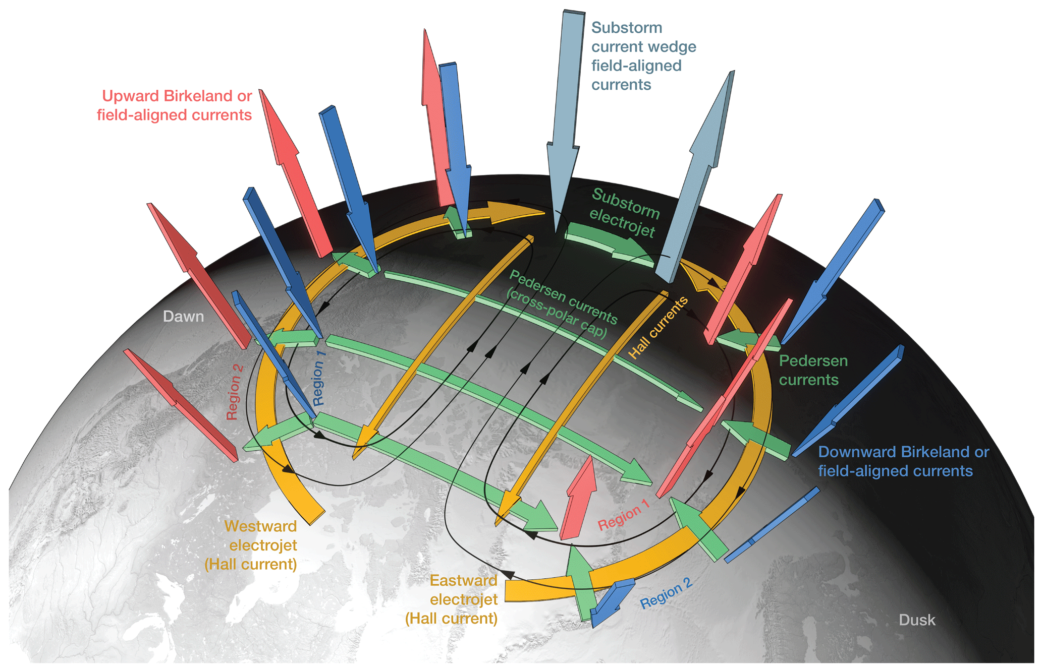
Figure 6Schematic view of the high-latitude ionospheric current system, showing the configuration of the driving field-aligned currents of Region 1 (along field lines closing via the outer magnetosphere) and Region 2 (closing via the opposite hemisphere). Also shown schematically are the locations and configuration of the ionospheric convection pattern, Pedersen and Hall currents, the substorm current wedge and auroral electrojets.
FAC current systems are also observed at smaller scales, of which auroral arcs provide the best example (Partamies et al., 2010). A recent review is provided by Karlsson et al. (2020). Within this example, the upward FAC sheet (consisting mainly of precipitating electrons) above the arc is paired with a downward FAC sheet (e.g. Elphic et al., 1998), similar to the scaled-down R1/R2 system. Multiple arcs can consist of multiple pairs of upward and downward FACs, but are also observed to share a unique current system, with all the arcs on the upward FAC leg (Wu et al., 2017). Another example of a scaled-down current system, similar to the substorm current wedge, is provided by the current circuit that connects magnetospheric bursty bulk flows (Baumjohann et al., 1990; Angelopoulos et al., 1992) with ionospheric north–south auroral structures (Henderson et al., 1998), also known as streamers. It has also been suggested that the substorm current wedge consists of several such wedgelets (Liu et al., 2015; recent review by Liu et al., 2018b).
Planar and filamentary FAC structures, connected by meridional and zonal ionospheric current, respectively, correspond to the two basic configurations of the auroral current circuit anticipated by Boström (1964), illustrated above with specific examples. Mixed configurations are observed as well; for instance, event studies (Marghitu et al., 2009, 2011) and statistical evidence (Jiang et al., 2015) suggest that a current system consisting of planar FAC sheets and ionospheric FAC closure in the zonal direction may develop during the substorm growth phase. A different kind of mixed configuration is observed for active Alfvénic arcs, where the planar FAC sheet can break into current filaments (Chaston et al., 2011). While sheets and filaments provide simple geometries, convenient for organising FACs according to their scales, actual observations are rarely clear-cut and reflect superpositions of geometries and scales, often more complex also than the two above examples of mixed configurations.
Various techniques have been developed to deal with actual FAC data, able to explore their multi-scale structure (e.g. Bunescu et al., 2015), or to take advantage of multi-point in situ information, as provided e.g. by the Cluster and Swarm missions (e.g. Dunlop et al., 2002; Marchaudon et al., 2009; Ritter et al., 2013; Blăgău and Vogt, 2019; Vogt et al., 2020). An alternative option, which benefits from prior development and validation with ground-based data, is the spherical elementary current systems (SECS) technique (Amm, 1997; Amm and Viljanen, 1999), adapted also for Swarm data (Amm et al., 2015). A key advantage of this approach is that, when used with LEO satellite data, it provides both the FACs and the ionospheric currents in a consistent manner (such that the FAC density is equal to the divergence of the curl-free ionospheric current). On the other hand, its accuracy and resolution depend on the distance above the ionospheric current, in particular for the divergence-free component (typically dominated by electrojet Hall current), whose effect is observed remotely. Statistical investigations of FAC and ionospheric currents, based on Swarm data, were published e.g. by Lühr et al. (2016), Huang et al. (2017), and Workayehu et al. (2019).
4.3 Poynting flux
The problem in assessing ionospheric energy deposition using ionospheric measurements only is that several elements need to be evaluated simultaneously so that the total dissipation can be assessed. A possible way to overcome this problem is to evaluate the total electromagnetic energy, i.e. the Poynting flux towards the ionosphere both using observations and numerical simulations. If this assessment can be carried out on high enough orbits, the assumption is that the Poynting flux includes both the energy dissipated in Joule heating as well as the energy within particle precipitation. The main caveat in this technique is to evaluate the magnetic field such that it does not contain contributions from the dipole, so that it represents the extra electromagnetic energy towards the ionosphere. Therefore, the field-aligned component of the Poynting vector can be evaluated from the quasi-static electric and perturbation magnetic fields E and δB measured above the ionosphere. In the limit of quasi-static planar current sheets, the Poynting flux can be shown to be equal to the Joule dissipation j⋅E integrated along the magnetic field line below the spacecraft (Kelley et al., 1991).
Studies of high-latitude Poynting flux have been carried out with DE-2 (Gary et al., 1994) and, more recently, Swarm (Park et al., 2017a; Pakhotin et al., 2018, 2020) missions. Rodríguez-Zuluaga et al. (2017) used Swarm to resolve magnetic-field-aligned Poynting flux at low latitudes with a resolution on the order of 1 µW m−2. Waters et al. (2004) introduced a method to characterise the high-latitude Poynting flux towards the ionosphere by combining electric field measurements of SuperDARN with the Iridium constellation estimating magnetic perturbations. This technique has the advantage of allowing the assessment of the net electromagnetic energy transferring to the ionosphere, including the energy deposited to drive the neutral winds, while not having to estimate the ionosphere conductivity. The technique presented in Waters et al. (2004) agrees with the DMSP satellite in situ measurement to a few mW m−2. They estimate the total electromagnetic energy flux on the order of 50 GW, maximising in the morning and afternoon sectors.
The topic is also ideal for global numerical simulations covering the entire solar-wind–magnetosphere–ionosphere system. These simulations can be used to assess the electric and magnetic fields within large volumes and map them to the ionospheric plane. In fact, global MHD simulations have shown that the Poynting flux starts to focus towards the magnetosphere and ionosphere already from the solar wind in regions where the open field lines are dragged towards the tail (Papadopoulos et al., 1999; Palmroth et al., 2003, 2006c). Zhang et al. (2012) used a global MHD simulation, mapped the Poynting flux in the tail to the ionosphere, and confirmed that its ionospheric distribution reproduced the global morphology of the Poynting flux measured by the Polar satellite. While these studies have been carried out using MHD simulations that have severe limitations in reproducing kinetic plasma physics within the magnetosphere, the results are indicative of processes that need to be rigorously measured so that our magnetosphere–ionosphere system can be understood in terms of an energy input/output system.
4.4 Ion–neutral cross sections
Of the derived parameters characterising the local properties of the LTI, among the most critical ones are the ion–neutral cross sections. Two types of ion–neutral cross sections will be briefly reviewed here: (i) the ion–neutral momentum-transfer cross sections and (ii) the ion–neutral chemical reaction cross sections.
Ion–neutral averaged momentum-transfer cross sections, which are denoted σcoll,in here, are needed to determine the ion–neutral collision frequencies (see Sect. 4.5). They are functions of velocity-dependent momentum-transfer cross sections and the relative velocity between particles. Using the velocity-dependent momentum-transfer cross-sectional expression derived by Dalgarno et al. (1958), Banks (1966) obtained the following formula for the averaged non-resonant ion–neutral momentum-transfer cross section:
with α the neutral gas atomic polarisability, e the elementary charge, μ the ion–neutral reduced mass, kB Boltzmann's constant, Ti and mi the ion temperature and mass, respectively, and Tn and mn the neutral temperature and mass, respectively. This formula was derived under the assumption that the ion–neutral interaction is predominantly due to the polarisation force arising from induced dipole attraction by the neutral gas, hence neglecting short-range quantum mechanical repulsion effects. This assumption holds for temperatures below 300 K, which is the order of magnitude of the temperature in the LTI (see Sect. 3.2). At higher altitudes, however, such as in the F region, the ion and neutral temperatures are well above this limit and start diverging. The dominant interaction in the F region is the charge exchange of the O+ ion with atomic oxygen O. The momentum-transfer cross section for O+ and O, , is dominated by the charge-exchange process, whereas the contribution from polarisation can be neglected in the F region (Banks, 1966). While the ion–neutral cross sections are crucial, they have never been measured within the LTI, and laboratory measurements reproducing the conditions in the upper atmosphere are extremely challenging (Lindsay et al., 2001). Therefore, the estimates of have been extrapolated from measurements and theoretical calculations at lower temperature, which are summarised in the introduction of Joshi et al. (2018).
The study of the ion–neutral interactions requires accurate measurements of plasma and neutral species in relevant partially ionised media, including composition of the neutral and ion species, velocity distribution of ions and electrons, as well as ambient energy that is characterised by electric and magnetic fields, radiation, and temperature. Since such complex environments, particularly under the influence of various electromagnetic fields and with complicated composition, temperature, and radiation fluxes, cannot easily be reproduced in a laboratory, the only way to understand the plasma–neutral gas interactions in space is through in situ observations in various environments in space (Yamauchi et al., 2019). Particularly, observations in low-density environments with substantial neutral particle content are needed, for example, in the upper ionosphere near the exobase of a planet or natural satellite, in comets, or in interstellar space.
Likewise, ion–neutral reaction cross sections, denoted σreac,in here, in the LTI are poorly known. They are also crucial as they affect the chemical reaction rates and hence are key parameters in upper-atmosphere models. Ion–neutral reaction cross sections have been derived from laboratory measurements of ion–molecule reaction rate constants in drift tubes (e.g. Woo and Wong, 1971), but those estimates suffer from two main problems: they can be energy-dependent, and simple ion–neutral relative speed distribution approximations do not hold in regions of the high-latitude LTI where ion convection speeds are high (St.-Maurice and Torr, 1978). In such cases, the rate coefficient k of a given reaction is given by
with f(v) the distribution of relative speeds v between the reactants. In this situation, σreac,in can be obtained by inverting k when the laboratory relative speed distribution flab(v) is known (St.-Maurice and Torr, 1978). Lin and Bardsley (1977) proposed a Monte Carlo method to derive flab(v) to serve this purpose. Using this methodology, the reaction cross sections for O+ with the main molecular species in the LTI (N2, O2 and NO) were published by Albritton et al. (1977) based on drift-tube experiments in both helium and argon buffer gases.
4.5 Ion–neutral collision frequencies
The collision rates for all species in the LTI constitute a fundamental set of parameters in the coupling in the atmosphere–ionosphere–magnetosphere system. They depend on a number of terms as shown below. Under the assumption that the ion and neutral populations in the LTI are separate Maxwellian distribution functions, the ion–neutral collision frequency νin can be expressed as (Banks, 1966)
with nn the neutral density, kB Boltzmann's constant, Ti and mi the ion temperature and mass, respectively, Tn and mn the neutral temperature and mass, respectively, and σcoll,in the ion–neutral collision cross section (see Sect. 4.4). From Eq. (6), one gets in the non-resonant case
which is an expression that has been used for space physics applications such as the analysis of incoherent scatter radar measurements (e.g. Virtanen et al., 2014). For a given ion–neutral pair, this can be further reduced as
with Cin a numerical coefficient whose value is given for relevant non-resonant ion–neutral pairs in the ionosphere by Schunk and Nagy (1980, see Table 6). Resonant charge-exchange interactions occur when a neutral and an ion from the same species collide with each other; the corresponding ion–neutral collision frequencies, which are also given in Schunk and Nagy (1980, see Table 5), depend on .
Besides laboratory experiment extrapolation to LTI conditions, ion–neutral collision frequencies have been estimated directly in the ionosphere using incoherent scatter radars. Nygrén et al. (1989) developed a method using the EISCAT radar to determine the ion–neutral collision frequency in the E region. It uses radar observations in the vertical, field-aligned and eastward-tilted directions to obtain measurements of the ion velocity and the electric field vector, which are used to infer νin from the momentum equation for the ions. This method was applied to estimate νin within 95–130 km altitude in Nygrén et al. (1989). It was used by Oyama et al. (2012) to study the temporal variations of the ion–neutral collision frequency within 106–135 km altitude during an ionospheric heating event. Alternative methods employing incoherent scatter radars to infer the ion–neutral collision frequency in the LTI can be found in Kosch et al. (2011), who combined incoherent scatter radar and optical observations to estimate νin in the vicinity of an auroral arc, as well as in Nicolls et al. (2014), who made use of multifrequency radar measurements to retrieve νin and estimate the thermospheric neutral density.
The ion–neutral collision frequency νin has been measured in situ only by sub-orbital rockets as they descended through the LTI (see Fig. 8 in Sangalli et al., 2009), and the measurement has never been conducted from a satellite. The rocket technique involves comparing the E×B drift velocity derived from the respective field measurements with direct measurements of the horizontal drift speed of ions (Watanabe et al., 1991). In the LTI, the two quantities differ by an amount that depends on the ratio where Ωi is the ion gyro-frequency. Accurate determination of κ also requires an independent measurement of the neutral wind velocity (Sangalli et al., 2009; Burchill et al., 2012). As such rocket measurements provide only a handful of observations, the ion–neutral collision frequencies remain poorly characterised, and their inferred values likely suffer from uncertainties. Collision cross sections and collision rates are among the largest sources of errors in empirical models, general circulation models, and magnetosphere–ionosphere coupling simulations, for which they are key inputs. Furthermore, they represent the largest source of uncertainty in estimating the ionospheric conductivities, which are key parameters in current coupled models of the LTI.
4.6 Ionospheric conductivities
Ionospheric conductivities are also particularly important derived local parameters, as they are required especially in modelling and further required to understand Joule heating. The ionospheric conductivity tensor is specified with the parallel conductivity σ∥ (along the magnetic field), the Pedersen conductivity σP (associated with ionospheric currents perpendicular to the geomagnetic field and parallel to the electric field defined in the reference frame moving with the conductive air at the speed of ambient neutral air in the bottomside ionosphere) and the Hall conductivity σH (associated with ionospheric currents perpendicular to both the electric and magnetic fields). Specifically, σP and σH are expressed as
with ne the electron density, e the elementary charge, νin the ion–neutral collision frequency (see Sect. 4.5), νen the electron–neutral collision frequency, mi and me the ion and electron masses, respectively, and Ωi and Ωe the ion and electron gyrofrequencies, respectively. Due to high electrical conductivity in the direction of the magnetic field, σ∥ is very large, up to tens of S m−1 (e.g. Yamazaki and Maute, 2017). This means that the geomagnetic field lines are nearly equipotential in the ionosphere, facilitating the approximation of the ionospheric parameters in the height-integrated form. As a consequence, the Pedersen and Hall conductivities are often presented as their height-integrated forms (i.e. conductances) as
The Pedersen and Hall conductivities and conductances can be estimated locally using incoherent scatter radar observations. Using the measured electron density profiles and expressions for the ion–neutral and electron–neutral collision frequencies such as given in Brekke and Hall (1988), Hall and Pedersen conductivity profiles can be derived and integrated across altitudes to obtain the corresponding conductances. Using this methodology, Aikio and Selkälä (2009) used the EISCAT radar to determine local conductances during a 1-month campaign and found that the conductances are larger in the morning sector than in the evening sector. The ionospheric conductivities can also be determined from spacecraft measurements using UV- and X-ray imaging of the aurora onboard polar-orbiting spacecraft (Aksnes et al., 2002, 2005).
In local numerical models, σP and σH are computed according to their definitions (Eqs. 11–12). However, large uncertainties exist regarding the values of the collision frequencies (νin and νen), and if electron density profiles are inaccurately reproduced, this can result in significant errors in the calculated conductivities. Ionospheric conductivities have been calculated using the TRANSCAR couple kinetic/fluid transport code (e.g. Lilensten et al., 1996), more recently making use of the AMIE procedure for multi-instrument data assimilation into the model (Blelly et al., 2005). In global magnetosphere–ionosphere coupling simulations, the conductivities are absolute key parameters and can have far-reaching effects if reproduced erroneously. Often the conductances consist of two parts, an empirically derived F10.7-dependent dayside part (e.g. Moen and Brekke, 1993), while the nightside conductances are often empirical formulations based on electron precipitation (e.g. Robinson et al., 1987). Even small changes in the conductances and e.g. adding seasonal variations can have tremendous effects in the overall modelling results (Ridley, 2007), and therefore their estimation in situ is of great importance.
4.7 Heating
The largest source of heating in the LTI is the absorption of solar EUV and UV radiation with an average rate of roughly 1 mW m−2 (Peterson et al., 2012) or globally a few hundred GW. The solar cycle modulates these values by about ±50 % (e.g. Lean et al., 2003). Furthermore, the heat flux maximises at the subsolar point and decreases away from it, in darkness to almost zero (except for a small contribution of Lyman α radiation originating from the geocorona; e.g. Maeda, 1969; Waldrop and Paxton, 2013).
Heating by electric currents, alternatively named frictional and Joule heating, is another important source. The Joule heating rate can be expressed locally as
with σP the Pedersen conductivity, E the electric field, u the neutral wind speed and B the magnetic field. The generated heat flux varies from insignificant to about 60 mW m−2, the estimated global power between about 1 GW and up to roughly 1 TW (Buchert, 2020; Fedrizzi et al., 2012; Sarris et al., 2020), although different methods suggest either large underestimations (Codrescu et al., 1995) or overestimations (Palmroth et al., 2005) within the measurements, while the exact values are not known. The ion–neutral frictional heating flux peaks during large geomagnetic storms (Lu et al., 2016). In such cases, JH surpasses the thermospheric heating by solar radiation, although on average the solar input is larger. However, JH rates, their spatial distribution, and temporal variations are relatively poorly determined, preventing more quantitative assessments.
The third source of heat is associated with particle precipitation which produces the aurora. The total heat flux produced by particle precipitation can range between 50 % and 100 % of that produced through Joule heating (Vickrey et al., 1982). Large particle precipitation energy fluxes tend to occur on small scales (visible as structures in the aurora); consequently, the energy flux associated with auroral particle precipitation can often surpass that of Joule heating locally. Virtanen et al. (2018) estimated corresponding values of up to 160 mW m−2.
Figure 7 shows the electron density, Pedersen conductivity and Joule heating rate in a TIE-GCM simulation of the LTI on 17 March 2015. The top row shows views above the North Pole, while the bottom row shows latitude–altitude cuts (in the direction indicated with red lines in the upper panels). Figure 7e and f indicate that both the Pedersen conductivity and the Joule heating rate maximise at about 120 km altitude, whereas Fig. 7b and c indicate that the global maxima of each parameter occurs at different local times. This illustrates the dependence of Joule heating not only on the Pedersen conductivity, but also on the electric fields, which can be very localised. The white stripes centred on 90∘ latitude in the bottom-row figures correspond to the region of 87.5–90∘ latitude where TIE-GCM does not give output.
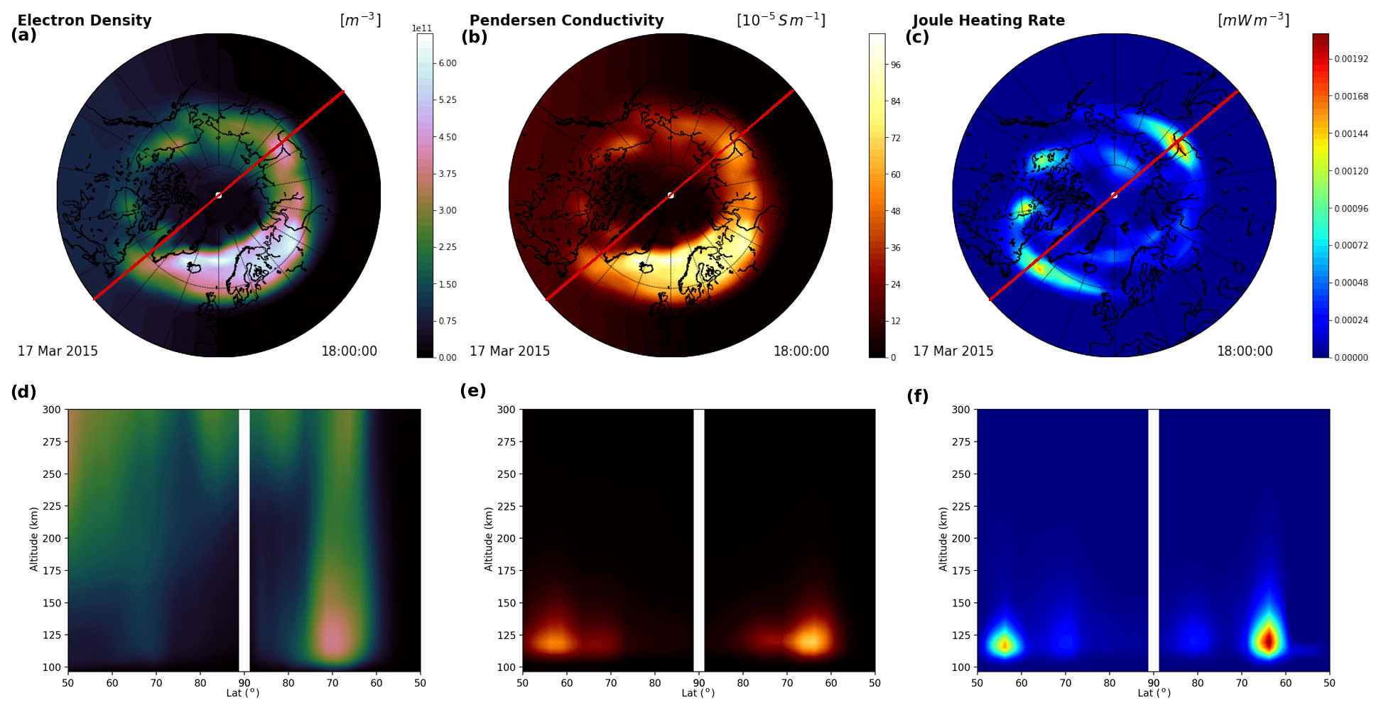
Figure 7Maps of (a) the electron density, (b) the Pedersen conductivity, and (c) the Joule heating rate at ∼ 120 km altitude on 17 March 2015 18:00:00 (UTC) based on TIE-GCM. (d) Electron density, (e) Pedersen conductivity, and (f) Joule heating rate as a function of geographic latitude and altitude in the plane indicated with a red line in the above panels.
4.8 Heat transfer to the neutral gas by ion and electron cooling
When the ion and electron temperatures, Ti and Te, respectively, are increased compared to the neutral temperature Tn, heat is transferred to the neutral gas by ion and electron cooling and also between ions and electrons. The corresponding steady-state heat transfer rate from ions to neutrals can be expressed as (e.g. Killeen et al., 1984)
with Ne the electron density, νin the ion–neutral collision frequency, mn the neutral mass, mi the ion mass, and kB Boltzmann's constant. Neglecting heat transfer from and to the light electrons, this heat transfer would (for similar ion and neutral compositions) amount to about half of the JH rate (Eq. 15), while the other half of the JH rate heats the neutrals directly.
The analogous expression for the heat transfer rate to the neutral gas by electron cooling, qΔT,e, is complicated by the numerous inelastic collisions between electrons and neutrals which are important for energy transfer. Comprehensive tables of relevant cross sections can be found in Schunk and Nagy (2009). Finally, above roughly 200 km altitude, ion-electron Coulomb collisions provide for significant heat exchange between ions and electrons when Ti≠Te.
In contrast to the external heating mechanisms discussed in Sect. 4.7, heat transfer between neutrals, ions, and electrons is an internal process in the LTI; hence, it is not associated with a heat source from the LTI perspective.
In practice, estimating the amount of heat transferred to the neutral gas requires coordinated measurements and subsequent modelling and can thus only be carried out in fortuitous conditions at specific locations, where measurements are available. Such conditions were met for instance in Marchaudon et al. (2018), who used simultaneous measurements from SuperDARN and EISCAT radars, ionosondes, the CHAMP satellite (Reigber et al., 2006), and subsequent modelling with the IPIM model (Marchaudon and Blelly, 2015) to investigate the mechanism behind the ionosphere F-peak electron density decrease at high latitudes during a high-speed stream event. They concluded that neutrals in the thermosphere were heated by up to 160 K during the studied event as a consequence of enhanced high-latitude convection, in agreement with earlier results by Gardner et al. (2012). However, Marchaudon et al. (2018) showed that the long-lasting ionospheric effects were due to the fact that this heating led to the expansion of the thermosphere and a change in the [O] [N2] ratio at the F-region peak altitude, which ultimately resulted in the extinction of the ionospheric F2 layer.
4.9 Atmospheric waves
Forcing from below can also affect the derived parameters within the LTI. The most important type of forcing from below is presented by gravity waves, which are excited by many meteorological processes (Fritts and Alexander, 2003) and which become increasingly prevalent at higher altitudes due to decreasing air density. The gravity waves, especially the ones with fast vertical speed, can penetrate into the LTI region and up to ∼ 200 km before they are dissipated by molecular damping. These meteorological processes, as well as tectonic activities and human-made explosions, can generate acoustic waves that propagate into the LTI region. Like gravity waves, the acoustic wave amplitudes increase with altitude and can thus cause large perturbations in the upper atmosphere (Walterscheid et al., 2003; Zettergren and Snively, 2013). These waves perturb the neutral winds and neutral and plasma temperatures and densities. Evidence of these waves, including travelling ionospheric disturbances (TIDs), have been observed in connection with tornados, deep convections, tsunamis, earthquakes, volcanos, and human-made explosions (Heki, 2006; Dautermann et al., 2009; Makela et al., 2011; Tsugawa et al., 2011; Nishioka et al., 2013; Azeem et al., 2015, 2018; Scott and Major, 2018), and it is one of the objectives of the proposed Daedalus mission to investigate the links between gravity waves and TIDs. Gravity waves may seed plasma instabilities, leading to the formation of equatorial spread F (Kelley et al., 1981; Hysell et al., 1990; Palmroth et al., 2000; Huba and Liu, 2020). High-resolution numerical simulations also suggest that gravity waves can produce large vertical wind shears above the mesopause, where the atmosphere is statistically the most stable (Liu, 2007, 2017). These wind shears can have important implications for E-region electrodynamics, including sporadic E layers (Mathews, 1998; Haldoupis, 2012).
Gravity wave dissipation, either due to wave breaking or molecular damping, causes heat and species transport (Walterscheid, 1981; Liu, 2000; Becker, 2004; Garcia et al., 2007; Liu, 2009; Gardner and Liu, 2010). This affects the transport within the LTI, its mass exchange with the mesosphere, and the compositional structure of the entire thermosphere. Acoustic waves can contribute to the thermospheric energetics through viscous heating (e.g. Hickey et al., 2001; Walterscheid and Hickey, 2005). In numerical models, such as WACCM-X and TIE-GCM, the thermospheric density, the O N2 ratio, and ionospheric plasma density are sensitively dependent on the effective eddy diffusion parameterised or specified in the mesosphere and lower thermosphere. For example, rather realistic semi-annual variation in thermospheric density was obtained by adjusting the eddy diffusion at the lower boundary of TIE-GCM (at ∼ 97 km) (Qian et al., 2009).
On global scales, tidal waves and fast-propagating planetary waves (e.g. ultra-fast Kelvin waves) and their variability can be an important cause of LTI variability. Like gravity waves, upward-propagating tides can reach up to ∼ 200 km before being largely dissipated by molecular damping and can cause large perturbations in wind, temperature, and composition in the LTI. Propagating tides are quantified by satellites, as outlined in a comprehensive review by Liu (2016). Recent studies have provided further evidence that the ionospheric day-to-day variability could be closely tied to the tidal day-to-day variability. For example, the pre-reversal enhancement of equatorial vertical E×B drift shows strong day-to-day variability. A recent analysis demonstrates that, through the E-region dynamo at midlatitudes in the summer hemisphere, the day-to-day variability of tidal winds plays a central role (Liu, 2020). It is also found that tidal winds determine the day-to-day variability of the equatorial vertical drift (Zhou et al., 2020).
In contrast to tides, the quantification of gravity waves and acoustic waves and of their effects in the LTI remains a challenge for both observations and numerical modelling, because of the scarcity of LTI observations in general, their multiscale nature (10 s–1000 s km) and relative high frequency, and their global distribution. The altitude range of most ground-based and satellite techniques for measuring perturbations associated with gravity waves is limited to below 100 km. A notable exception is lidar measurements of metal layers, which can sometimes reach up to ∼ 170 km (Chu et al., 2016, and references therein). However, the occurrence of such metal layers is sporadic, and it is challenging to obtain horizontal information, long-term variation, and global distribution of the waves from these measurements. Two new NASA satellite missions, GOLD (Eastes et al., 2017) and ICON (Immel et al., 2018), make remote measurements in the LTI region, around 160 and 100–160 km, respectively. LTI gravity wave information can potentially be extracted from their measurements. With the scarcity of direct gravity wave measurements in LTI, low-altitude in situ measurements would be extremely valuable. At the same time, global measurements of gravity waves in the mesosphere, for example by the upcoming NASA Atmosphere Wave Explorer (AWE, https://www.nasa.gov/press-release/, last access: 22 February 2021), will be highly complementary in linking the waves in the LTI to lower atmospheric sources.
4.10 Total electron content and derived quantities
The total electron content (TEC) refers to the integrated electron density ne along the line of sight between a receiver and a satellite-borne transmitter: . It can be derived from the measurements of two carrier wave frequencies (f1,f2) transmitted by GNSS satellites:
where L1 and L2 are carrier-phase observations, K is a constant, DCBt and DCBr are differential code biases of the transmitter and receiver, respectively, and Δϵ accounts for ambiguities due to cycle slip corrections and remaining errors. sTEC is the slant TEC related to the actual number of electrons between the transmitter and receiver. It depends on the elevation angle of the GNSS satellite as the ray path through ionospheric layers with higher electron density gets longer for lower elevations. By using an adequate mapping function, the vertical TEC, vTEC, can be obtained (e.g. Noja et al., 2013; Zhang et al., 2016; Montenbruck and Rodríguez, 2020; Jin et al., 2019). For ground-based receivers, it is often assumed that the pierce point of the ionosphere is at 350 km, and a thin, shell-like ionospheric model is used for obtaining vTEC. However, for a receiver onboard another satellite above the pierce point, often a more advanced mapping function assuming a thick ionosphere should be used (Noja et al., 2013). More complex approaches for vTEC are also typically used in tomography techniques (e.g. Meggs et al., 2004). Note that additional biases in TEC measurements, such as receiver temperature, may contribute to errors in TEC estimations (Coster et al., 2013). The concepts of ground-based sTEC and its mapping to vTEC are shown in Fig. 8a.
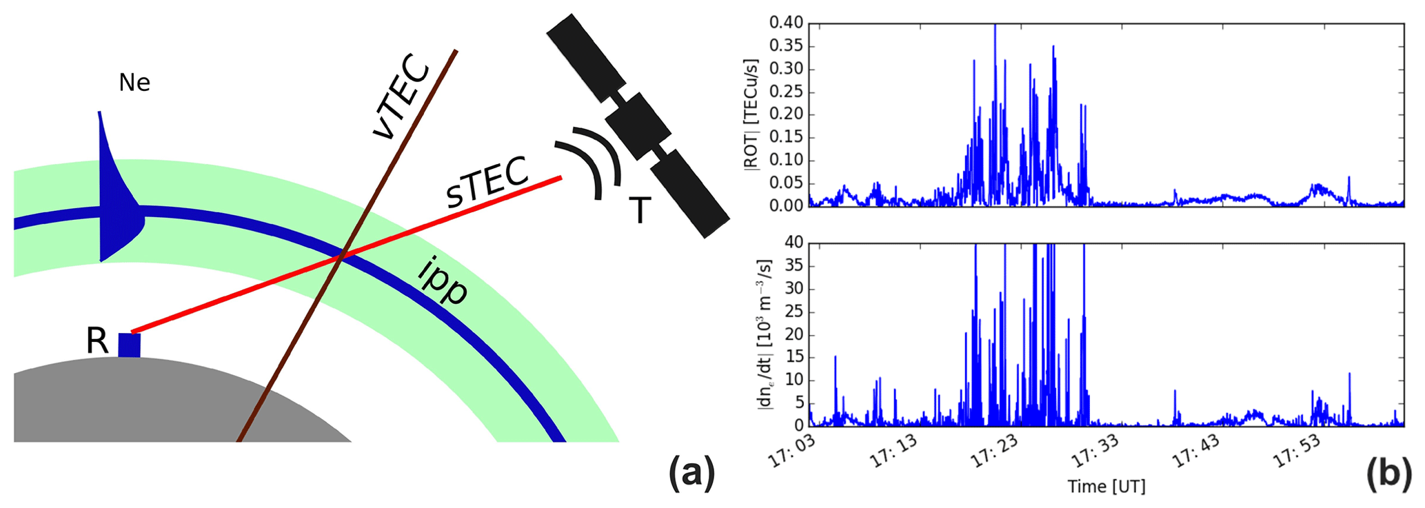
Figure 8(a) Schematics of obtaining sTEC and vTEC; T: transmitter, R: receiver, Ne: electron density profile in the ionosphere, IPP: ionospheric pierce point. (b) Example of ROT and electron density variations (absolute values) as measured by Swarm A during 1 h on 8 September 2017.
TEC is nowadays routinely used for monitoring electron density variations in the ionosphere. It is generally displayed as 2D maps based on networks of ground-based receivers (Coster et al., 1992). Over the years, TEC has successfully been used for studies of the response of the ionosphere to geomagnetic storms (Danilov, 2013; Mendillo, 2006), but also to study dynamics of ionospheric structures such as polar cap patches or travelling ionospheric disturbances (Tsugawa et al., 2004; Durgonics et al., 2017). In numerical simulations which model the LTI, TEC is naturally obtained by integrating the computed electron density along a (slanted or vertical) path. Similarly, from tomographic reconstructions of the ionosphere (e.g. Norberg et al., 2015), TEC can be obtained by numerical integration of the inverted electron density. In such cases, additional measurements than solely from GNSS, such as ISR or ionosonde observations, can be used to feed the tomographic inversion system and therefore contribute to the TEC derivation. One example of such an assimilative tomography network is TomoScand in Fennoscandia (e.g. Norberg et al., 2018).
Ground-based networks used for TEC calculations are limited in coverage, in particular in the polar regions and over oceans. This limitation can be addressed by GNSS receivers onboard LEO satellites. Such satellite-based measurements of the topside ionosphere TEC have recently provided an additional highly valuable contribution, by characterising structures, density gradients and irregularities in ionospheric plasma (e.g. Chartier et al., 2018; Jin et al., 2019). They further support in situ plasma density measurements, as they do not only follow similar characteristics in the context of structuring (Zakharenkova et al., 2016; Xiong et al., 2016; Jin et al., 2019), but they also add additional information about the directional extent of plasma density variations (e.g. Park et al., 2017b; Follestad et al., 2020). Thus TEC, together with in situ plasma density measurements, gives a detailed insight into scales of plasma density structures, gradients, and the overall plasma density variations. A large number of tracked GNSS satellites by a receiver onboard LEO satellites can even provide insight into the spatial extent of structures in the ionosphere, such as polar cap patches, equatorial spread F, and auroral blobs, when using inversion methods (Follestad et al., 2020).
Derived TEC parameters, such as the rate of change of TEC (ROT), being the temporal derivative of TEC, and the ROT index (ROTI), being the standard deviation of ROT in a given time interval, provide important characterisation of plasma irregularities in the topside ionosphere. It has been shown that satellite-based TEC variations are correlated with the in situ measurements of plasma density variations (Xiong et al., 2016). Indeed, due to the shape of ionospheric density profiles, the largest contribution to TEC comes from plasma in the vicinity of the LEO satellite. Thus, ROT and ROTI are closely related to the variability in the local ionospheric plasma density (Jin et al., 2019; Xiong et al., 2016); see also Fig. 8b. As such, they can also be related to the quality of trans-ionospheric radio signals, and since TEC is derived from the measurements of GNSS signals, these measurements can also give insight into processes behind ionospheric scintillations, especially if the receiver provides high-frequency data.
TEC and other GNSS-related measurements depend on the electron density variations in the topside ionosphere and hence on the satellite's orbit. The peak of the ionospheric F layer, which gives the largest contribution to the variations in the signal propagation, is below the altitudes of most LEO satellites. A low-perigee satellite mission embedding a high-frequency GNSS receiver onboard could allow for the first time the probing of different contributions to TEC, in particular from different parts of the F region and upper E region of the ionosphere or from the plasmasphere, and related variability, and as such it could provide a unique opportunity to investigate the effect of plasma irregularities on the GNSS signals at different altitudes.
There are at least four viewpoints from which understanding of the LTI is crucial: scientific, policy-based, technological, and from the perspective of the society at large. First and foremost, humans explore – not only our own planet, but also celestial and astronomical bodies within and beyond our solar system. It is astonishing that we can find a region so near to the surface of our planet −80 to 200 km altitude – which is still part of the so-called ignorosphere due to the lack of systematic in situ measurements. Since the LTI is shown to influence atmospheric and climate systems, it should be understood as part of our planetary system. In fact, from this perspective the entire near-Earth space linking to the LTI belongs to the Earth system. Even so, the LTI and the near-Earth space are often regarded as fall-betweens as the understanding of their phenomena requires knowledge from atmospheric physics, chemistry and space physics. This multitude of fields should not hinder us in exploring the LTI; on the contrary, the inherent interdisciplinary nature should challenge us to think about the region from many different scientific perspectives.
Policymakers are continually interested in the climate system due to climate change and its anthropogenic nature. From the climate change perspective, as described in Sect. 2.3, it is imperative to understand the role of electron precipitation within the natural polar climate variability to accurately quantify the contribution due to human activities. Understanding the LTI is a key element in this endeavour. However, policymakers have recently also been pushing towards getting prepared for possible large space weather events, as e.g. the European Union, the United Kingdom, and the United States of America have issued reports on this matter (see e.g. Cabinet Office, 2017; Executive Office of the President of the United States, 2019). The goal is to develop mitigation strategies to protect human infrastructure from the potentially devastating impact that a major geomagnetic storm could have. The current understanding of geospace still contains some gaps that preclude predictive simulations of the effects to be anticipated from a given solar storm. One such gap is related to the LTI, whose complexity comes from the intertwined behaviours of its neutral and ionised components which are governed by distinct physical processes and from its couplings to below and above. A major difficulty lies in that it proves extremely challenging to measure physical parameters at LTI altitudes, both through in situ instruments and via remote observations.
From a technological perspective, the reason why the LTI lies within the ignorosphere is because the exploration of the region is so difficult. Spacecraft on circular low-Earth orbits experience thermal problems and return to Earth due to the increased drag. Remote-sensing methods require some emission to be gathered by the remote instrument, but there are regions within the LTI which do not emit these signals (Sarris, 2019). Ground-based measurements such as the incoherent scatter radars are invaluable in describing the ionised part of the LTI. However, due to the coupled nature of the LTI, it is necessary to explore several other regions such as the magnetotail simultaneously, which is of course extremely challenging to achieve in a systematic way. Therefore, the exploration of the LTI needs to be understood as a coordinated effort from the beginning. However, due to the difficulties involved, a mission obtaining systematic in situ measurements of the LTI would be a great technological achievement comparable to exploring the deepest seas and the furthest galaxies.
In this review, open questions related to the LTI have been divided according to three viewpoints: energetics, variability and dynamics, and chemistry. From the perspective of energetics, large uncertainties exist in estimating the relative contributions of the various sources of energy (solar radiation flux, Joule heating, particle precipitation, atmospheric waves, exothermic chemical reactions) under various contexts (latitude, local time, season, geomagnetic activity, solar cycle), which makes the determination of the LTI energy budget very challenging. Regarding variability and dynamics, the understanding of the complex couplings of the LTI with the magnetosphere and the underlying neutral atmosphere is still limited. This is not only true at high latitudes, where substorms create large effects, but also at low latitudes where the equatorial electrojet and plasma irregularities play a large role. Finally, the LTI chemistry involves a great number of species, whose densities are determined by temperature-dependent photochemical reactions and by production rates associated with particle precipitation. However, many of the critical parameters, such as the ion–neutral cross sections and collision rates, remain poorly characterised.
To address the unanswered science questions pertaining to the LTI, additional observations of its key parameters, ideally in situ, are needed in various regions of interest. In the ionospheric E region, interest is in the equatorial electrojet region, corresponding to geomagnetic latitudes (MLAT) comprised within, roughly, , and the auroral latitudes, comprised in most situations within 60–75∘. In the F region, the areas of interest encompass all latitudes and include, in particular the equatorial plasma bubble region (within MLAT, 18:00–04:00 MLT), midlatitude Sq currents (within MLAT, 06:00–19:00 MLT), auroral latitudes, the polar cusp regions on the dayside (70–80∘ MLAT, 10:00–14:00 MLT), and the polar cap region ( MLAT). Ideally, systematic observations in these regions should cover a wide range of seasons and geomagnetic conditions to enable the study of their effects on the LTI energetics, variability, dynamics, and chemistry.
Systematic in situ observations of the key LTI parameters (precipitating particle fluxes and energy spectra, ion and neutral temperatures, compositions and densities, neutral winds, ion drift speeds and electric fields, and magnetic fields) could allow the derivation of physical quantities, knowledge of which is crucial for the correct modelling of the LTI and its external drivers. For instance, the forcing from above consists not only of particle precipitation, but also of the Lorentz force exerted onto the ions, of field-aligned currents, and of the Poynting flux, which all need to be taken into account while developing boundary conditions for ionospheric models. Microscopic parameters such as the ion–neutral cross sections, collision frequencies, and heat transfer coefficients are also needed in the kinetic transport and photochemical modules of ionospheric models. Furthermore, supercomputing centres are becoming increasingly accessible to research groups, and hence space environment modelling is expected to make significant steps towards understanding and forecasting space weather. The increased amount of available computing power also enables assimilative schemes to incorporate more data, as is currently done using the AMIE technique for ground-based radar and satellite observations (Cousins et al., 2015). All these models benefit from systematic in situ observations, leading to a reduction of uncertainties and errors in numerical simulations.
Finally, a phenomenon that continually interests society at large is the beautiful and vivid auroral displays that take place in the LTI. For example, a recent citizen science auroral discovery, named the dunes, reached 2.5 billion people all around the world in just two weeks after publication (Palmroth et al., 2020). This discovery followed a similar one by a collaboration between Canadian amateur photographers and space physicists, which revealed the phenomenon nowadays known as strong thermal emission velocity enhancement (STEVE; MacDonald et al., 2018; Gallardo-Lacourt et al., 2018) associated with the smallest-scale optical emissions in the night sky reported so far (Semeter et al., 2020) and which has reached even larger numbers describing public interest. All the above-mentioned features pertaining to the LTI – its role as a region to be explored, the technological challenges it poses, and its role within worldwide policies combined with the fascinating aurora and other optical features – make it an ideal topic for a wide range of stories to engage the public at large, generating increased interest in natural sciences and possibly giving new opportunities for citizen science studies (Grandin, 2020). For these reasons, a dedicated satellite mission providing regular observations of the key LTI parameters is highly desirable and timely.
| The list below contains the abbreviations corresponding to satellite missions, | |
| ground-based instruments, numerical models, and abbreviations used | |
| repeatedly throughout the article. | |
| AE-B/C | Atmosphere Explorer B/C |
| AMIE | Assimilative Mapping of Ionospheric Electrodynamics |
| CHAMP | Challenging Minisatellite Payload |
| DE-2 | Dynamics Explorer-2 |
| DMSP | Defense Meteorological Satellite Program |
| EISCAT | European Incoherent Scatter |
| EMIC | Electromagnetic ion cyclotron |
| EPP | Energetic particle precipitation |
| ESA | European Space Agency |
| EUV | Extreme ultraviolet |
| FAC | Field-aligned current |
| FPI | Fabry–Perot interferometer |
| GNSS | Global navigation satellite system |
| GOCE | Gravity Field and Steady-State Ocean Circulation Explorer |
| GOLD | Global-scale Observations of the Limb and Disk |
| GPS | Global Positioning System |
| HF | High frequency |
| HWM | Horizontal Wind Model |
| ICON | Ionosphere CONnection Explorer |
| IDM | Ion-drift meter |
| IMF | Interplanetary magnetic field |
| IPIM | IRAP Plasmasphere–Ionosphere model |
| IRI | International Reference Ionosphere |
| ISR | Incoherent scatter radar |
| JH | Joule heating |
| LEO | Low-Earth orbit |
| LTI | Lower thermosphere–ionosphere |
| MHD | Magnetohydrodynamic |
| MIT | Magnetosphere–ionosphere–thermosphere |
| MLAT | Magnetic latitude |
| MLT | Magnetic local time |
| NASA | National Aeronautics and Space Administration |
| NOAA | National Oceanic and Atmospheric Administration |
| POES | Polar-orbiting Operational Environmental Satellite |
| ROT | Rate of change of TEC |
| ROTI | ROT index |
| RPA | Retarding potential analyser |
| SAPS | Subauroral polarisation streams |
| SDI | Scanning Doppler imager |
| sTEC | Slant TEC |
| SuperDARN | Super Dual Auroral Radar Network |
| TEC | Total electron content |
| TID | Travelling ionospheric disturbance |
| TIE-GCM | Thermosphere Ionosphere Electrodynamics General Circulation Model |
| UTC | Universal Time Coordinate |
| UV | Ultraviolet |
| vTEC | Vertical TEC |
| WACCM | Whole Atmosphere Community Climate Model |
| WACCM-D | Whole Atmosphere Community Climate Model with D-region ion chemistry |
| WACCM-X | Whole Atmosphere Community Climate Model with thermosphere and ionosphere extension |
The DMSP data used to make Fig. 3a are provided by NOAA and can be downloaded from the DMSP/SSJ archives at https://satdat.ngdc.noaa.gov/dmsp/data/ (Redmon, 2021). Figure 3b was made using OvationPyme, the Python implementation of Ovation Prime 2010, which is available at https://github.com/lkilcommons/OvationPyme (Kilcommons, 2021). The NRLMSISE-00 and IRI-2012 models used to produce Fig. 4 are available online through NASA's Community Coordinated Modeling Center (CCMC) at https://ccmc.gsfc.nasa.gov/modelweb/models/nrlmsise00.php (Papitashvili, 2021) and https://ccmc.gsfc.nasa.gov/modelweb/models/iri2012_vitmo.php (Papitashvili and Rastaetter, 2021), respectively. Data from the Swarm mission visualised in Figs. 5 and 8b are provided by ESA via http://swarm-diss.eo.esa.int (ESA, 2021) or ftp://swarm-diss.eo.esa.int. TIE-GCM model run data shown in Figs. 7 and 2b were produced at the Democritus University of Thrace, with AMIE inputs provided by Gang Lu, NCAR/HAO. WACCM-X model run data used to generate Figs. 1 and 2 were produced at NCAR/HAO, provided by Federico Gasperini. Both datasets are available from the author TS on request, while run requests of TIE-GCM can be made via the CCMC at https://ccmc.gsfc.nasa.gov/models/modelinfo.php?model=TIE-GCM (Garcia-Sage et al., 2021) and the WACCM-X code can be downloaded as part of the Community Earth System Model version 2 http://www.cesm.ucar.edu/models/cesm2/ (Faircloth, 2021).
The writing of this article was led by MP and coordinated by MG, with contributions from all the co-authors. ED made Figs. 1, 2, and 6. MG made Fig. 3, RP made Fig. 4, ClS and NO made Fig. 5, TS and ST made Fig. 7, WM made Fig. 8. Significant contributions to the text by section are as follows: 1: MP; 2.1: MP, SB, HLL; 2.2: MP, DMM, CSt, MY; 2.3: MP, PTV, MAC, MG; 3.1: MG, AK; 3.2: PV, GM, MG; 3.3: ID, PV, MG; 3.4: GM, GK, MG, ED; 3.5: AM, AA, DJK, MP; 3.6: ClS, NO; 4.1: OM, MP, TMJ, DJK; 4.2: DJK, TMJ, OM, MP, MG; 4.3: MP, DJK; 4.4: MG, MY; 4.5: MG, DJK; 4.6: TM, MG, AA; 4.7: SB, MG; 4.8: SB, MG; 4.9: HLL, MP; 4.10: WM, ChS, JvdIJ, MG; 5: MG, MP.
The authors declare that they have no conflict of interest.
The authors thank Federico Gasperini (NCAR/HAO) for providing the WACCM-X model output visualised in Figs. 1 and 2 and Gang Lu (NCAR/HAO) for providing AMIE high-latitude forcing input for the model simulations.
This research has been supported by the European Space Agency (ESA/ESTEC) contract number 4000127346/19/NL/IA with the Democritus University of Thrace for the Daedalus science and requirements consolidation study, in the framework of the Earth Explorer 10 Phase-0 feasibility studies (PI: Theodoros Sarris). Further support was provided by the European Space Agency (grant nos. 4000127660 MAGICS, and 4000118383 SIFACIT), the European Research Council (grant no. 682068-PRESTISSIMO), the Academy of Finland, Luonnontieteiden ja Tekniikan Tutkimuksen Toimikunta (grant nos. 309937 and 312351), the National Science Foundation, USA (grant nos. 1852977, OPP-1443726, and AGS-1552153), NASA (grant nos. NNX16AB82G, 80NSSC20K0601, 80NSSC20K0633, and 80NSSC17K0007), the Research Council of Norway (grant nos. 267408 and 275653), and the Programme National Soleil-Terre de l'Institut des Sciences de l'Univers (PNST/INSU).
This paper was edited by Georgios Balasis and reviewed by two anonymous referees.
Aikio, A. T. and Selkälä, A.: Statistical properties of Joule heating rate, electric field and conductances at high latitudes, Ann. Geophys., 27, 2661–2673, https://doi.org/10.5194/angeo-27-2661-2009, 2009. a
Aikio, A. T., Lakkala, T., Kozlovsky, A., and Williams, P. J. S.: Electric fields and currents of stable drifting auroral arcs in the evening sector, J. Geophys. Res.-Space, 107, SIA 3–1–SIA 3–14, https://doi.org/10.1029/2001JA009172, 2002. a
Aikio, A. T., Mursula, K., Buchert, S., Forme, F., Amm, O., Marklund, G., Dunlop, M., Fontaine, D., Vaivads, A., and Fazakerley, A.: Temporal evolution of two auroral arcs as measured by the Cluster satellite and coordinated ground-based instruments, Ann. Geophys., 22, 4089–4101, https://doi.org/10.5194/angeo-22-4089-2004, 2004. a
Aikio, A. T., Vanhamäki, H., Workayehu, A. B., Virtanen, I. I., Kauristie, K., Juusola, L., Buchert, S., and Knudsen, D.: Swarm Satellite and EISCAT Radar Observations of a Plasma Flow Channel in the Auroral Oval Near Magnetic Midnight, J. Geophys. Res.-Space, 123, 5140–5158, https://doi.org/10.1029/2018JA025409, 2018. a, b
Akasofu, S. I.: Energy coupling between the solar wind and the magnetosphere., Space Sci. Rev., 28, 121–190, https://doi.org/10.1007/BF00218810, 1981. a
Akmaev, R. A., Fuller-Rowell, T. J., Wu, F., Forbes, J. M., Zhang, X., Anghel, A. F., Iredell, M. D., Moorthi, S., and Juang, H. M.: Tidal variability in the lower thermosphere: Comparison of Whole Atmosphere Model (WAM) simulations with observations from TIMED, Geophys. Res. Lett., 35, L03810, https://doi.org/10.1029/2007GL032584, 2008. a
Aksnes, A., Stadsnes, J., Bjordal, J., Østgaard, N., Vondrak, R. R., Detrick, D. L., Rosenberg, T. J., Germany, G. A., and Chenette, D.: Instantaneous ionospheric global conductance maps during an isolated substorm, Ann. Geophys., 20, 1181–1191, https://doi.org/10.5194/angeo-20-1181-2002, 2002. a
Aksnes, A., Stadsnes, J., Lu, G., Østgaard, N., Vondrak, R. R., Detrick, D. L., Rosenberg, T. J., Germany, G. A., and Schulz, M.: Effects of energetic electrons on the electrodynamics in the ionosphere, Ann. Geophys., 22, 475–496, https://doi.org/10.5194/angeo-22-475-2004, 2004. a
Aksnes, A., Amm, O., Stadsnes, J., Østgaard, N., Germany, G. A., Vondrak, R. R., and Sillanpää, I.: Ionospheric conductances derived from satellite measurements of auroral UV and X-ray emissions, and ground-based electromagnetic data: a comparison, Ann. Geophys., 23, 343–358, https://doi.org/10.5194/angeo-23-343-2005, 2005. a
Albritton, D. L., Dotan, I., Lindinger, W., McFarland, M., Tellinghuisen, J., and Fehsenfeld, F. C.: Effects of ion speed distributions in flow-drift tube studies of ion-neutral reactions, J. Chem. Phys., 66, 410–421, https://doi.org/10.1063/1.433986, 1977. a
Alken, P.: Observations and modeling of the ionospheric gravity and diamagnetic current systems from CHAMP and Swarm measurements, J. Geophys. Res., 121, 589–601, https://doi.org/10.1002/2015JA022163, 2016. a
Alken, P. and Maus, S.: Spatio-temporal characterization of the equatorial electrojet from CHAMP, Orsted, and SAC-C satellite magnetic measurements, J. Geophys. Res., 112, A09305, https://doi.org/10.1029/2007JA012524, 2007. a
Alken, P., Maute, A., and Richmond, A. D.: The F-Region Gravity and Pressure Gradient Current Systems: A Review, Space Sci. Rev., 206, 451–469, https://doi.org/10.1007/s11214-016-0266-z, 2017. a
Amm, O.: Ionospheric elementary current systems in spherical coordinates and their applications, J. Geomagn. Geoelectr., 49, 947–955, 1997. a
Amm, O. and Viljanen, A.: Ionospheric disturbance magnetic field continuation from the ground to the ionosphere using spherical elementary current systems, Earth Planet. Space, 51, 431–440, https://doi.org/10.1186/BF03352247, 1999. a
Amm, O., Vanhamäki, H., Kauristie, K., Stolle, C., Christiansen, F., Haagmans, R., Masson, A., Taylor, M. G. G. T., Floberghagen, R., and Escoubet, C. P.: A method to derive maps of ionospheric conductances, currents, and convection from the Swarm multisatellite mission, J. Geophys. Res.-Space, 120, 3263–3282, https://doi.org/10.1002/2014JA020154, 2015. a
Anderson, B. J., Korth, H., Waters, C. L., Green, D. L., Merkin, V. G., and Dyrud, L. P.: Development of large-scale Birkeland currents determined from the Active Magnetosphere and Planetary Electrodynamics Response Experiment, Geophys. Res. Lett., 41, 3017–3025, https://doi.org/10.1002/2014GL059941, 2014. a
Anderson, J. D.: Fundamentals of aerodynamics, McGraw-Hill, fifth edition, McGraw-Hill Education, 2010. a
Anderson, P. C., Heelis, R. A., and Hanson, W. B.: The ionospheric signatures of rapid subauroral ion drifts, J. Geophys. Res.-Space, 96, 5785–5792, https://doi.org/10.1029/90JA02651, 1991. a
Andersson, M. E., Verronen, P. T., Marsh, D. R., Päivärinta, S.-M., and Plane, J. M. C.: WACCM-D – Improved modeling of nitric acid and active chlorine during energetic particle precipitation, J. Geophys. Res.-Atmos., 121, 10328–10341, https://doi.org/10.1002/2015JD024173, 2016. a
Andersson, M. E., Verronen, P. T., Marsh, D. R., Seppälä, A., Päivärinta, S.-M., Rodger, C. J., Clilverd, M. A., Kalakoski, N., and van de Kamp, M.: Polar Ozone Response to Energetic Particle Precipitation Over Decadal Time Scales: The Role of Medium-Energy Electrons, J. Geophys. Res.-Atmos., 123, 607–622, https://doi.org/10.1002/2017JD027605, 2018. a
Angelopoulos, V., Baumjohann, W., Kennel, C. F., Coroniti, F. V., Kivelson, M. G., Pellat, R., Walker, R. J., Lühr, H., and Paschmann, G.: Bursty bulk flows in the inner central plasma sheet, J. Geophys. Res., 97, 4027–4039, https://doi.org/10.1029/91JA02701, 1992. a
Angelopoulos, V., Kennel, C. F., Coroniti, F. V., Pellat, R., Kivelson, M. G., Walker, R. J., Russell, C. T., Baumjohann, W., Feldman, W. C., and Gosling, J. T.: Statistical characteristics of bursty bulk flow events, J. Geophys. Res., 99, 21257–21280, https://doi.org/10.1029/94JA01263, 1994. a
Angelopoulos, V., McFadden, J. P., Larson, D., Carlson, C. W., Mende, S. B., Frey, H., Phan, T., Sibeck, D. G., Glassmeier, K.-H., Auster, U., Donovan, E., Mann, I. R., Rae, I. J., Russell, C. T., Runov, A., Zhou, X.-Z., and Kepko, L.: Tail Reconnection Triggering Substorm Onset, Science, 321, 931, https://doi.org/10.1126/science.1160495, 2008. a, b
Annadurai, N. M. N., Hamid, N. S. A., Yamazaki, Y., and Yoshikawa, A.: Investigation of Unusual Solar Flare Effect on the Global Ionospheric Current System, J. Geophys. Res.-Space, 123, 8599–8609, https://doi.org/10.1029/2018JA025601, 2018. a
Archer, M. O., Horbury, T. S., Brown, P., Eastwood, J. P., Oddy, T. M., Whiteside, B. J., and Sample, J. G.: The MAGIC of CINEMA: first in-flight science results from a miniaturised anisotropic magnetoresistive magnetometer, Ann. Geophys., 33, 725–735, https://doi.org/10.5194/angeo-33-725-2015, 2015. a
Archer, W. E., Knudsen, D. J., Burchill, J. K., Jackel, B., Donovan, E., Connors, M., and Juusola, L.: Birkeland current boundary flows, J. Geophys. Res.-Space, 122, 4617–4627, https://doi.org/10.1002/2016JA023789, 2017. a
Aruliah, A. L., Griffin, E. M., Yiu, H.-C. I., McWhirter, I., and Charalambous, A.: SCANDI – an all-sky Doppler imager for studies of thermospheric spatial structure, Ann. Geophys., 28, 549–567, https://doi.org/10.5194/angeo-28-549-2010, 2010. a
Asikainen, T. and Mursula, K.: Correcting the NOAA/MEPED energetic electron fluxes for detector efficiency and proton contamination, J. Geophys. Res.-Space, 118, 6500–6510, https://doi.org/10.1002/jgra.50584, 2013. a
Axford, W. I. and Hines, C. O.: A unifying theory of high-latitude geophysical phenomena and geomagnetic storms, Can. J. Phys., 39, 1433–1464, 1961. a
Azeem, I., Yue, J., Hoffmann, L., Miller, S. D., Straka III, W. C., and Crowley, G.: Multisensor profiling of a concentric gravity wave event propagating from the troposphere to the ionosphere, Geophys. Res. Lett., 42, 7874–7880, https://doi.org/10.1002/2015GL065903, 2015. a
Azeem, I., Walterscheid, R. L., and Crowley, G.: Investigation of Acoustic Waves in the Ionosphere Generated by a Deep Convection System Using Distributed Networks of GPS Receivers and Numerical Modeling, Geophys. Res. Lett., 45, 8014–8021, https://doi.org/10.1029/2018GL078107, 2018. a
Baker, D. N., Mason, G. M., Figueroa, O., Colon, G., Watzin, J. G., and Aleman, R. M.: An overview of the Solar, Anomalous, and Magnetospheric Particle Explorer (SAMPEX) mission, IEEE T. Geosci. Remote, 31, 531–541, https://doi.org/10.1109/36.225519, 1993. a
Balsiger, H., Altwegg, K., Bochsler, P., Eberhardt, P., Fischer, J., Graf, S., Jäckel, A., Kopp, E., Langer, U., Mildner, M., Müller, J., Riesen, T., Rubin, M., Scherer, S., Wurz, P., Wüthrich, S., Arijs, E., Delanoye, S., de Keyser, J., Neefs, E., Nevejans, D., Rème, H., Aoustin, C., Mazelle, C., Médale, J. L., Sauvaud, J. A., Berthelier, J. J., Bertaux, J. L., Duvet, L., Illiano, J. M., Fuselier, S. A., Ghielmetti, A. G., Magoncelli, T., Shelley, E. G., Korth, A., Heerlein, K., Lauche, H., Livi, S., Loose, A., Mall, U., Wilken, B., Gliem, F., Fiethe, B., Gombosi, T. I., Block, B., Carignan, G. R., Fisk, L. A., Waite, J. H., Young, D. T., and Wollnik, H.: Rosina Rosetta Orbiter Spectrometer for Ion and Neutral Analysis, Space Sci. Rev., 128, 745–801, https://doi.org/10.1007/s11214-006-8335-3, 2007. a, b
Banks, P.: Collision frequencies and energy transfer. Ions, Planet. Space Sci., 14, 1105–1122, https://doi.org/10.1016/0032-0633(66)90025-0, 1966. a, b, c
Bates, D. R.: Some problems concerning the terrestrial atmosphere above about the 100 km level, P. R. Soc. London, A253, 451–462, https://doi.org/10.1098/rspa.1959.0207, 1959. a
Baumgaertner, A. J. G., Seppälä, A., Jöckel, P., and Clilverd, M. A.: Geomagnetic activity related NOx enhancements and polar surface air temperature variability in a chemistry climate model: modulation of the NAM index, Atmos. Chem. Phys., 11, 4521–4531, https://doi.org/10.5194/acp-11-4521-2011, 2011. a
Baumjohann, W.: Ionospheric and field-aligned current systems in the auroral zone: A concise review, Adv. Space Res., 2, 55–62, 1983. a
Baumjohann, W., Paschmann, G., and Lühr, H.: Characteristics of high‐speed ion flows in the plasma sheet, J. Geophys. Res., 95, 3801–3809, https://doi.org/10.1029/JA095iA04p03801, 1990. a
Beaussier, J., Mainguy, A.-M., Olivero, A., and Rolland, R.: In orbit performance of the Cactus accelerometer (D5B spacecraft), Acta Astronaut., 4, 1085–1102, https://doi.org/10.1016/0094-5765(77)90008-X, 1977. a
Becker, E.: Direct heating rates associated with gravity wave saturation, J. Atmos. Terr. Phys., 66, 683–696, 2004. a
Becker, E.: Mean-Flow Effects of Thermal Tides in the Mesosphere and Lower Thermosphere, J. Atmos. Sci., 74, 2043–2063, https://doi.org/10.1175/JAS-D-16-0194.1, 2017. a
Beig, G.: Review of mesospheric temperature trends, Rev. Geophys., 41, 1015, https://doi.org/10.1029/2002RG000121, 2003. a
Beig, G., Scheer, J., Mlynczak, M. G., and Keckhut, P.: Overview of the temperature response in the mesosphere and lower thermosphere to solar activity, Rev. Geophys., 46, RG3002, https://doi.org/10.1029/2007RG000236, 2008. a
Belakhovsky, V., Pilipenko, V., Murr, D., Fedorov, E., and Kozlovsky, A.: Modulation of the ionosphere by Pc5 waves observed simultaneously by GPS/TEC and EISCAT, Earth Planet. Space, 68, 102, https://doi.org/10.1186/s40623-016-0480-7, 2016. a
Berger, M. J., Seltzer, S. M., and Maeda, K.: Energy deposition by auroral electrons in the atmosphere, J. Atmos. Terr. Phys., 32, 1015–1045, https://doi.org/10.1016/0021-9169(70)90115-7, 1970. a
Bi, Y., Chen, Y., Zhou, R., Yi, M., and Deng, S.: Simulation of the effect of water-vapor increase on temperature in the stratosphere, Adv. Atmos. Sci., 28, 832–842, https://doi.org/10.1007/s00376-010-0047-7, 2011. a
Bilitza, D. and Reinisch, B. W.: International Reference Ionosphere 2007: Improvements and new parameters, Adv. Space Res., 42, 599–609, https://doi.org/10.1016/j.asr.2007.07.048, 2008. a
Bilitza, D., Altadill, D., Zhang, Y., Mertens, C., Truhlik, V., Richards, P., McKinnell, L.-A., and Reinisch, B.: The International Reference Ionosphere 2012 - a model of international collaboration, J. Space Weather Spac., 4, A07, https://doi.org/10.1051/swsc/2014004, 2014. a
Bilitza, D., Altadill, D., Truhlik, V., Shubin, V., Galkin, I., Reinisch, B., and Huang, X.: International Reference Ionosphere 2016: From ionospheric climate to real-time weather predictions, Adv. Space Res. 15, 418–429, https://doi.org/10.1002/2016SW001593, 2017. a
Billett, D. D., Hosokawa, K., Grocott, A., Wild, J. A., Aruliah, A. L., Ogawa, Y., Taguchi, S., and Lester, M.: Multi-Instrument Observations of Ion-Neutral Coupling in the Dayside Cusp, Geophys. Res. Lett., 47, e85590, https://doi.org/10.1029/2019GL085590, 2020. a
Birkeland, K.: The norwegian aurora polaris expedition, 1902-03, vol. 1, First Section, Aschehoug and Co., Christiania, 1908. a
Birn, J., Hesse, M., Haerendel, G., Baumjohann, W., and Shiokawa, K.: Flow braking and the substorm current wedge, J. Geophys. Res., 104, 19895–19903, https://doi.org/10.1029/1999JA900173, 1999. a
Blelly, P.-L., Fontanari, J., Alcayde, D., Wu, J., Blanc, M., and Hansen, T. L.: Observations of the structure and vertical transport of the polar upper ionosphere with the EISCAT-VHF radar. III - Topside neutral composition and quiet-time temperature, Annales Geophysicae, 10, 394–406, 1992. a
Blelly, P.-L., Lathuillère, C., Emery, B., Lilensten, J., Fontanari, J., and Alcaydé, D.: An extended TRANSCAR model including ionospheric convection: simulation of EISCAT observations using inputs from AMIE, Ann. Geophys., 23, 419–431, https://doi.org/10.5194/angeo-23-419-2005, 2005. a
Blelly, P. L., Alcaydé, D., and van Eyken, A. P.: A new analysis method for determining polar ionosphere and upper atmosphere characteristics from ESR data: Illustration with IPY period, J. Geophys. Res.-Space, 115, A09322, https://doi.org/10.1029/2009JA014876, 2010. a
Blăgău, A. and Vogt, J.: Multipoint field-aligned current estimates with Swarm, J. Geophys. Res.-Space, 124, 6869–6895, https://doi.org/10.1029/2018JA026439, 2019. a
Blum, L., Li, X., and Denton, M.: Rapid MeV electron precipitation as observed by SAMPEX/HILT during high-speed stream-driven storms, J. Geophys. Res.-Space, 120, 3783–3794, https://doi.org/10.1002/2014JA020633, 2015. a
Boström, R.: A model of the auroral electrojets, J. Geophys. Res., 69, 4983–4999, 1964. a, b, c
Brasseur, G. P. and Solomon, S.: Aeronomy of the Middle Atmosphere, Springer, Dordrecht, 3rd revised and enlarged edn., 2005. a
Brattli, A., Lie-Svendsen, Ø., Svenes, K., Hoppe, U.-P., Strelnikova, I., Rapp, M., Latteck, R., and Friedrich, M.: The ECOMA 2007 campaign: rocket observations and numerical modelling of aerosol particle charging and plasma depletion in a PMSE/NLC layer, Ann. Geophys., 27, 781–796, https://doi.org/10.5194/angeo-27-781-2009, 2009. a
Brekke, A. and Hall, C.: Auroral ionospheric quiet summer time conductances, Annales Geophysicae, 6, 361–375, 1988. a
Bruinsma, S.: The DTM-2013 thermosphere model, J. Space Weather Spac., 5, A1, https://doi.org/10.1051/swsc/2015001, 2015. a
Buchert, S. C.: Entangled dynamos and Joule heating in the Earth's ionosphere, Ann. Geophys., 38, 1019–1030, https://doi.org/10.5194/angeo-38-1019-2020, 2020. a
Bunescu, C., Marghitu, O., Constantinescu, D., Narita, Y., Vogt, J., and Blăgău, A.: Multiscale field-aligned current analyzer, J. Geophys. Res.-Space, 120, 9563–9577, https://doi.org/10.1002/2015JA021670, 2015. a
Burch, J. L., Reiff, P. H., Menietti, J. D., Heelis, R. A., Hanson, W. B., Shawhan, S. D., Shelley, E. G., Sugiura, M., Weimer, D. R., and Winningham, J. D.: IMF By-dependent plasma flow and Birkeland currents in the dayside magnetosphere 1. Dynamics Explorer observations, J. Geophys. Res.-Space, 90, 1577–1594, https://doi.org/10.1029/JA090iA02p01577, 1985. a
Burch, J. L., Moore, T. E., Torbert, R. B., and Giles, B. L.: Magnetospheric Multiscale Overview and Science Objectives, Space Sci. Rev., 199, 5–21, https://doi.org/10.1007/s11214-015-0164-9, 2016. a
Burchill, J. K., Clemmons, J. H., Knudsen, D. J., Larsen, M., Nicolls, M. J., Pfaff, R. F., Rowland, D., and Sangalli, L.: High-latitudeEregion ionosphere-thermosphere coupling: A comparative study using in situ and incoherent scatter radar observations, J. Geophys. Res.-Space, 117, A02301, https://doi.org/10.1029/2011JA017175, 2012. a
Burrage, M. D., Skinner, W. R., Marshall, A. R., Hays, P. B., Lieberman, R. S., Franke, S. J., Gell, D. A., Ortland, D. A., Morton, Y. T., Schmidlin, F. J., Vincent, R. A., and Wu, D. L.: Comparison of HRDI wind measurements with radar and rocket observations, Geophys. Res. Lett., 20, 1259–1262, https://doi.org/10.1029/93GL01108, 1993. a
Cabinet Office: National Risk Register Of Civil Emergencies, https://assets.publishing.service.gov.uk/government/uploads/system/uploads/attachment_data/file/644968/UK_National_Risk_Register_2017.pdf (last access: 18 June 2020), 2017. a
Caudal, G. and Blanc, M.: The spatial distribution of magnetospheric convection electric fields at ionospheric altitudes - A review. I - Observations, Annales Geophysicae, 1, 519–526, 1983. a
Chappell, C. R.: The terrestrial plasma source: a new perspective in solar-terrestrialprocesses from Dynamics Explorer., Rev. Geophys., 26, 229–248, https://doi.org/10.1029/RG026i002p00229, 1988. a
Chartier, A. T., Mitchell, C. N., and Miller, E. S.: Annual Occurrence Rates of Ionospheric Polar Cap Patches Observed Using Swarm, J. Geophys. Res.-Space, 123, 2327–2335, https://doi.org/10.1002/2017JA024811, 2018. a
Chaston, C. C., Seki, K., Sakanoi, T., Asamura, K., Hirahara, M., and Carlson, C. W.: Cross-scale coupling in the auroral acceleration region, Geophys. Res. Lett., 38, L20101, https://doi.org/10.1029/2011GL049185, 2011. a
Cheng, M., Tapley, B., Bettadpur, S., and Ries, J.: Determination of thermospheric winds from grace accelerometer data, Adv. Astron. Sci., 130, 1181–1192, 2008. a
Chisham, G., Lester, M., Milan, S. E., Freeman, M. P., Bristow, W. A., Grocott, A., McWilliams, K. A., Ruohoniemi, J. M., Yeoman, T. K., Dyson, P. L., Greenwald, R. A., Kikuchi, T., Pinnock, M., Rash, J. P. S., Sato, N., Sofko, G. J., Villain, J. P., and Walker, A. D. M.: A decade of the Super Dual Auroral Radar Network (SuperDARN): scientific achievements, new techniques and future directions, Surv. Geophys., 28, 33–109, https://doi.org/10.1007/s10712-007-9017-8, 2007. a
Chu, X., Yu, Z., Fong, W., Chen, C., Zhao, J., Barry, I. F., Smith, J. A., Lu, X., Huang, W., and Gardner, C. S.: From Antarctica lidar discoveries to OASIS exploration, EPJ Web of Conferences, 119, 12001, https://doi.org/10.1051/epjconf/201611912001, 2016. a
Clilverd, M. A., Rodger, C. J., Thomson, N. R., Brundell, J. B., Ulich, T., Lichtenberger, J., Cobbett, N., Collier, A. B., Menk, F. W., SeppäLä, A., Verronen, P. T., and Turunen, E.: Remote sensing space weather events: Antarctic-Arctic Radiation-belt (Dynamic) Deposition-VLF Atmospheric Research Konsortium network, Adv. Space Res., 7, 04001, https://doi.org/10.1029/2008SW000412, 2009. a
Codrescu, M., J. Fuller-Rowell, T., and Foster, J.: On the importance of E-field variability for Joule heating in the high-latitude thermosphere, Geophys. Res. Lett. 22, 2393–2396, https://doi.org/10.1029/95GL01909, 1995. a, b
Codrescu, M. V., Fuller-Rowell, T. J., Roble, R. G., and Evans, D. S.: Medium energy particle precipitation influences on the mesosphere and lower thermosphere, J. Geophys. Res., 102, 19977–19988, 1997. a
Connor, H. K., Raeder, J., Sibeck, D. G., and Trattner, K. J.: Relation between cusp ion structures and dayside reconnection for four IMF clock angles: OpenGGCM-LTPT results, J. Geophys. Res.-Space, 120, 4890–4906, https://doi.org/10.1002/2015JA021156, 2015. a
Coster, A., Williams, J., Weatherwax, A., Rideout, W., and Herne, D.: Accuracy of GPS total electron content: GPS receiver bias temperature dependence, Radio Sci., 48, 190–196, https://doi.org/10.1002/rds.20011, 2013. a
Coster, A. J., Gaposchkin, E. M., and Thornton, L. E.: Real-time ionospheric monitoring system using GPS, Navigation, 39, 191–204, 1992. a
Cousins, E. D. P. and Shepherd, S. G.: A dynamical model of high-latitude convection derived from SuperDARN plasma drift measurements, J. Geophys. Res.-Space, 115, A12329, https://doi.org/10.1029/2010JA016017, 2010. a
Cousins, E. D. P., Matsuo, T., and Richmond, A. D.: Mapping high-latitude ionospheric electrodynamics with SuperDARN and AMPERE, J. Geophys. Res.-Space, 120, 5854–5870, https://doi.org/10.1002/2014JA020463, 2015. a, b
Cowley, S. W. H. and Lockwood, M.: Excitation and decay of solar wind-driven flows in the magnetosphere-ionophere system, Annales Geophysicae, 10, 103–115, 1992. a
Coxon, J. C., Milan, S. E., and Anderson, B. J.: A revies of Birkeland current research using AMPERE, in: Electric currents in Geospace and beyond, edited by: Keiling, A., Marghiu, O., and Wheatland, M., Geophysical Monograph 235, 257–278, AGU and Wiley, Washington, D.C., https://doi.org/10.1002/9781119324522.ch16, 2018. a
Crooker, N. U.: Dayside merging and cusp geometry, J. Geophys. Res.-Space, 84, 951–959, https://doi.org/10.1029/JA084iA03p00951, 1979. a
Cummings, W. D. and Dessler, A. J.: Field-aligned currents in the magnetosphere, J. Geophys. Res., 72, 1007–1013, 1967. a
Curto, J. J., Amory-Mazaudier, C., Torta, J. M., and Menvielle, M.: Solar flare effects at Ebre: Regular and reversed solar flare effects, statistical analysis (1953 to 1985), a global case study and a model of elliptical ionospheric currents, J. Geophys. Res., 99, 3945–3954, https://doi.org/10.1029/93JA02270, 1994. a
Dahlgren, H., Lanchester, B. S., Ivchenko, N., and Whiter, D. K.: Electrodynamics and energy characteristics of aurora at high resolution by optical methods, J. Geophys. Res.-Space, 121, 5966–5974, https://doi.org/10.1002/2016JA022446, 2016. a
Dalgarno, A., McDowell, M. R. C., and Williams, A.: The Mobilities of Ions in Unlike Gases, Philos. T. R. Soc. Lond., 250, 411–425, https://doi.org/10.1098/rsta.1958.0002, 1958. a
Damiani, A., Funke, B., Santee, M. L., Cordero, R. R., and Watanabe, S.: Energetic particle precipitation: A major driver of the ozone budget in the Antarctic upper stratosphere, Geophys. Res. Lett., 43, 3554–3562, https://doi.org/10.1002/2016GL068279, 2016. a
Dandouras, I., Yamauchi, M., De Keyser, J., Marghitu, O., Rème, H., Yoshikawa, I., Sakanoi, T., and the ESCAPE proposal team: ESCAPE: a mission proposal for ESA-M5 to systematically study Exosphere and atmospheric escape using European, Japanese, and US instruments, in: ISAS Symposium, S10-001, 9–10 January 2018 Sagamihara, Kanagawa, Japan, https://repository.exst.jaxa.jp/dspace/handle/a-is/876320, 2018 (in Japanese with English abstract). a
Dandouras, I., Blanc, M., Fossati, L., Gerasimov, M., Guenther, E. W., Kislyakova, K. G., Lammer, H., Lin, Y., Marty, B., Mazelle, C., Rugheimer, S., Scherf, M., Sotin, M., Sproß, L., Tachibana, S., Wurz, P., and Yamauchi, M.: Future Missions related to the determination of the elemental and isotopic composition of Earth, Moon and planets, Space Sci. Rev., 216, 121, https://doi.org/10.1007/s11214-020-00736-0, 2020. a
Danilov, A.: Ionospheric F-region response to geomagnetic disturbances, Adv. Space Res., 52, 343–366, https://doi.org/10.1016/j.asr.2013.04.019, 2013. a
Dautermann, T., Calais, E., and Mattioli, G. S.: Global Positioning System detection and energy estimation of the ionospheric wave caused by the 13 July 2003 explosion of the Soufrière Hills Volcano, Montserrat, J. Geophys. Res.-Sol. Ea., 114, B02202, https://doi.org/10.1029/2008JB005722, 2009. a
de Jesus, R., Fagundes, P., Coster, A., Bolaji, O., Sobral, J., Batista, I., de Abreu, A., Venkatesh, K., Gende, M., Abalde, J., and Sumod, S.: Effects of the intense geomagnetic storm of September–October 2012 on the equatorial, low- and mid-latitude F region in the American and African sector during the unusual 24th solar cycle, J. Atmos. Sol.-Terr. Phy., 138–139, 93–105, https://doi.org/10.1016/j.jastp.2015.12.015, 2016. a
Deng, W., Killeen, T. L., Burns, A. G., and Roble, R. G.: The flywheel effect: ionospheric currents after a geomagneic storm, Geophys. Res. Lett., 18, 1845–1848, 1991. a
Deng, W., Killeen, T. L., Burns, A. G., Roble, R. G., Slavin, J., and Wharton, L.: The effects of neutral inertia on ionospheric currents in the high-latitude thermosphere following a geomagneic storm, J. Geophys. Res., 98, 7775–7790, 1993. a
Dhadly, M. S., Meriwether, J., Conde, M., and Hampton, D.: First ever cross comparison of thermospheric wind measured by narrow- and wide-field optical Doppler spectroscopy, J. Geophys. Res.-Space, 120, 9683–9705, https://doi.org/10.1002/2015JA021316, 2015. a
Dombeck, J., Cattell, C., Prasad, N., Meeker, E., Hanson, E., and McFadden, J.: Identification of Auroral Electron Precipitation Mechanism Combinations and Their Relationships to Net Downgoing Energy and Number Flux, J. Geophys. Res.-Space, 123, 10064–10089, https://doi.org/10.1029/2018JA025749, 2018. a
Doornbos, E.: Thermospheric density and wind determination from satellite dynamics, PhD thesis, Delft Univ. of Technol., Delft, ISBN 978-90-9026051-8, 2011. a, b, c, d
Doornbos, E., Klinkrad, H., and Visser, P.: Use of two-line element data for thermosphere neutral density model calibration, Adv. Space Res., 41, 1115–1122, https://doi.org/10.1016/j.asr.2006.12.025, 2008. a
Doornbos, E., van den IJssel, J., Lühr, H., Foerster, M., Koppenwallner, G., Bruinsma, S., Sutton, E., Forbes, J. M., Marcos, F., and Perosanz, F.: Neutral Density and Crosswind Determination from Arbitrarily Oriented Multiaxis Accelerometers on Satellites, J. Spacecraft Rockets, 47, 580–589, https://doi.org/10.2514/1.48114, 2010. a
Drob, D. P., Emmert, J. T., Crowley, G., Picone, J. M., Shepherd, G. G., Skinner, W., Hays, P., Niciejewski, R. J., Larsen, M., She, C. Y., Meriwether, J. W., Hernandez, G., Jarvis, M. J., Sipler, D. P., Tepley, C. A., O'Brien, M. S., Bowman, J. R., Wu, Q., Murayama, Y., Kawamura, S., Reid, I. M., and Vincent, R. A.: An empirical model of the Earth's horizontal wind fields: HWM07, J. Geophys.Res.-Space, 113, A12304, https://doi.org/10.1029/2008JA013668, 2008. a
Drob, D. P., Emmert, J. T., Meriwether, J. W., Makela, J. J., Doornbos, E., Conde, M., Hernandez, G., Noto, J., Zawdie, K. A., McDonald, S. E., Huba, J. D., and Klenzing, J. H.: An update to the Horizontal Wind Model (HWM): The quiet time thermosphere, Earth Space Sci., 2, 301–319, https://doi.org/10.1002/2014EA000089, 2015. a, b
Dungey, J. W.: Interplanetary Magnetic Field and the Auroral Zones, Phys. Rev. Lett., 6, 47–48, https://doi.org/10.1103/PhysRevLett.6.47, 1961. a, b
Dunlop, M. W., Balogh, A., Glassmeier, K.-H., and Robert, P.: Four-point Cluster application of magnetic field analysis tools: The Curlometer, J. Geophys. Res.-Space, 107, 1384, https://doi.org/10.1029/2001JA005088, 2002. a
Durgonics, T., Komjathy, A., Verkhoglyadova, O., Shume, E. B., Benzon, H.-H., Mannucci, A. J., Butala, M. D., Høeg, P., and Langley, R. B.: Multiinstrument observations of a geomagnetic storm and its effects on the Arctic ionosphere: A case study of the 19 February 2014 storm, Radio Sci., 52, 146–165, https://doi.org/10.1002/2016RS006106, 2017. a
Eastes, R. W., McClintock, W. E., Burns, A. G., Anderson, D. N., Andersson, L., Codrescu, M., Correira, J. T., Daniell, R. E., England, S. L., Evans, J. S., Harvey, J., Krywonos, A., Lumpe, J. D., Richmond, A. D., Rusch, D. W., Siegmund, O., Solomon, S. C., Strickland, D. J., Woods, T. N., Aksnes, A., Budzien, S. A., Dymond, K. F., Eparvier, F. G., Martinis, C. R., and Oberheide, J.: The Global-Scale Observations of the Limb and Disk (GOLD) Mission, Space Sci. Rev., 212, 383–408, https://doi.org/10.1007/s11214-017-0392-2, 2017. a
Elphic, R. C., Bonnell, J. W., Strangeway, R. J., Kepko, L., Ergun, R. E., McFadden, J. P., Carlson, C. W., Peria, W., Cattell, C. A., Klumpar, D., Shelley, E., Peterson, W., Möbius, E., Kistler, L., and Pfaff, R.: The auroral current circuit and field-aligned currents observed by FAST, Geophys. Res. Lett., 25, 2033–2036, 1998. a
Emmert, J. T., Picone, J. M., and Meier, R. R.: Thermospheric global average density trends, 1967–2007, derived from orbits of 5000 near-Earth objects, Geophys. Res. Lett., 35, L05101, https://doi.org/10.1029/2007GL032809, 2008. a
Emmert, J. T., Stevens, M. H., Bernath, P. F., Drob, D. P., and Boone, C. D.: Observations of increasing carbon dioxide concentration in Earth's thermosphere, Nat. Geosci., 5, 868–871, https://doi.org/10.1038/ngeo1626, 2012. a
Engebretson, M. J., Posch, J. L., Capman, N. S. S., Campuzano, N. G., Bělik, P., Allen, R. C., Vines, S. K., Anderson, B. J., Tian, S., Cattell, C. A., Wygant, J. R., Fuselier, S. A., Argall, M. R., Lessard, M. R., Torbert, R. B., Moldwin, M. B., Hartinger, M. D., Kim, H., Russell, C. T., Kletzing, C. A., Reeves, G. D., and Singer, H. J.: MMS, Van Allen Probes, GOES 13, and Ground-Based Magnetometer Observations of EMIC Wave Events Before, During, and After a Modest Interplanetary Shock, J. Geophys. Res.-Space, 123, 8331–8357, https://doi.org/10.1029/2018JA025984, 2018. a
ESA: Swarm Data Access, available at: http://swarm-diss.eo.esa.int, last access: 22 February 2021.
Escoubet, C. P., Fehringer, M., and Goldstein, M.: Introduction The Cluster mission, Ann. Geophys., 19, 1197–1200, https://doi.org/10.5194/angeo-19-1197-2001, 2001. a
Executive Office of the President of the United States: National Space Weather Strategy and Action Plan, https://aerospace.org/sites/default/files/2019-03/Natl_Space_Weather_Strategy_Mar19.pdf (last access: 22 February 2021), 2019. a
Faircloth, E.: Community Earth System Model CESM2, available at: http://www.cesm.ucar.edu/models/cesm2/, last access: 22 February 2021.
Fedrizzi, M., Fuller-Rowell, T. J., and Codrescu, M. V.: Global Joule heating index derived from thermospheric density physics-based modeling and observations, Adv. Space Res, 10, S03001, https://doi.org/10.1029/2011SW000724, 2012. a
Finlay, C. C., Olsen, N., Kotsiaros, S., Gillet, N., and Tøffner-Clausen, L.: Recent geomagnetic secular variation from Swarm and ground observatories as estimated in the CHAOS-6 geomagnetic field model, Earth Planet. Space, 68, 112, https://doi.org/10.1186/s40623-016-0486-1, 2016. a
Fok, M.-C., Moore, T. E., Wilson, G. R., Perez, J. D., Zhang, X. X., Brandt, P. C., Mitchell, D. G., Roelof, E. C., Jahn, J.-M., Pollock, C. J., and Wolf, R. A.: Global ENA IMAGE Simulations, in: Magnetospheric Imaging — The Image Prime Mission, edited by: Burch, J. L., Springer Netherlands, Dordrecht, https://doi.org/10.1007/978-94-010-0027-7_5, 77–103, 2003. a
Follestad, A. F., Clausen, L. B. N., Miloch, W. J., van den Ijssel, J., and Haagmans, R.: Two dimensional reconstruction of ionospheric plasma density variations using Swarm, Adv. Space Res., 18, e2019SW002406, https://doi.org/10.1029/2019SW002406, 2020. a, b
Fomichev, V. I., Shved, G. M., and Kutepov, A. A.: Radiative cooling of the 30 – 110 km atmospheric layer., J. Atmos. Terr. Phy., 48, 529–544, https://doi.org/10.1016/0021-9169(86)90087-5, 1986. a
Foster, J. C.: An empirical electric field model derived from Chatanika radar data, J. Geophys. Res.-Space, 88, 981–988, https://doi.org/10.1029/JA088iA02p00981, 1983. a
Frey, H. U., Mende, S. B., Angelopoulos, V., and Donovan, E. F.: Substorm onset observations by IMAGE-FUV, J. Geophys. Res.-Space , 109, A10304, https://doi.org/10.1029/2004JA010607, 2004. a
Friis-Christensen, E., Lühr, H., and Hulot, G.: Swarm: A constellation to study the Earth's magnetic field, Earth Planet. Space, 58, 351–358, 2006. a
Friis-Christensen, E., Lühr, H., Knudsen, D., and Haagmans, R.: Swarm – An Earth Observation Mission investigating Geospace, Adv. Space Res., 41, 210–216, https://doi.org/10.1016/j.asr.2006.10.008, 2008. a
Fritts, D. C. and Alexander, M. J.: Gravity wave dynamics and effects in the middle atmosphere, Rev. Geophys., 41, 1003, https://doi.org/10.1029/2001RG000106, 2003. a
Fujii, R., Amm, O., Yoshikawa, A., Ieda, A., and Vanhamäki, H.: Reformulation and energy flow of the Cowling channel, J. Geophys. Res.-Space, 116, A02305, https://doi.org/10.1029/2010JA015,989, 2011. a
Fukizawa, M., Sakanoi, T., Miyoshi, Y., Hosokawa, K., Shiokawa, K., Katoh, Y., Kazama, Y., Kumamoto, A., Tsuchiya, F., Miyashita, Y., Tanaka, Y. M., Kasahara, Y., Ozaki, M., Matsuoka, A., Matsuda, S., Hikishima, M., Oyama, S., Ogawa, Y., Kurita, S., and Fujii, R.: Electrostatic Electron Cyclotron Harmonic Waves as a Candidate to Cause Pulsating Auroras, Geophys. Res. Lett., 45, 12661–12668, https://doi.org/10.1029/2018GL080145, 2018. a
Fuller-Rowell, T. J.: The Dynamics of the Lower Thermosphere, in: The Upper Mesosphere and Lower Thermosphere: A Review of Experiment and Theory, edited by: Johnson, R. M. and Killeen, T. L., American Geophysical Union (AGU),, Washington DC, https://doi.org/10.1029/GM087p0023, 23–36, 2013. a
Funke, B., López-Puertas, M., Holt, L., Randall, C. E., Stiller, G. P., and von Clarmann, T.: Hemispheric distributions and interannual variability of NOy produced by energetic particle precipitation in 2002–2012, J. Geophys. Res., 119, 13565–13582, https://doi.org/10.1002/2014JD022423, 2014. a
Galand, M.: Introduction to special section: Proton precipitation into the atmosphere, J. Geophys. Res., 106, 1–6, https://doi.org/10.1029/2000JA002015, 2001. a
Gallardo-Lacourt, B., Liang, J., Nishimura, Y., and Donovan, E.: On the Origin of STEVE: Particle Precipitation or Ionospheric Skyglow?, Geophys. Res. Lett., 45, 7968–7973, https://doi.org/10.1029/2018GL078509, 2018. a
Garcia, R. R., Marsh, D. R., Kinnison, D. E., Boville, B. A., and Sassi, F.: Simulation of secular trends in the middle atmosphere, 1950-2003, J. Geophys. Res.-Atmos., 112, D09301, https://doi.org/10.1029/2006JD007485, 2007. a
Garcia-Sage, K., Yue, J., Foster, B., and Solomon, S.: Thermosphere Ionosphere Electrodynamics General Circulation Model, available at: https://ccmc.gsfc.nasa.gov/models/modelinfo.php?model=TIE-GCM, last access: 22 February 2021.
Gardner, C. S. and Liu, A. Z.: Wave-induced transport of atmospheric constituents and its effect on the mesospheric Na layer, J. Geophys. Res.-Atmos., 115, D20302, https://doi.org/10.1029/2010JD014140, 2010. a
Gardner, L., Sojka, J. J., Schunk, R. W., and Heelis, R.: Changes in thermospheric temperature induced by high-speed solar wind streams, J. Geophys. Res.-Space, 117, A12303, https://doi.org/10.1029/2012JA017892, 2012. a
Gary, J. B., Heelis, R. A., Hanson, W. B., and Slavin, J. A.: Field-aligned Poynting Flux observations in the high-latitude ionosphere, J. Geophys. Res.-Space, 99, 11417–11427, https://doi.org/10.1029/93JA03167, 1994. a
Gettelman, A., Mills, M. J., Kinnison, D. E., Garcia, R. R., Smith, A. K., Marsh, D. R., Tilmes, S., Vitt, F., Bardeen, C. G., McInerny, J., Liu, H.-L., Solomon, S. C., Polvani, L. M., Emmons, L. K., Lamarque, J.-F., Richter, J. H., Glanville, A. S., Bacmeister, J. T., Phillips, A. S., Neale, R. B., Simpson, I. R., DuVivier, A. K., Hodzic, A., and Randel, W. J.: The Whole Atmosphere Community Climate Model Version 6 (WACCM6), J. Geophys. Res.-Atmos., 124, 12380–12403, https://doi.org/10.1029/2019JD030943, 2019. a
Glocer, A., Fok, M., Meng, X., Toth, G., Buzulukova, N., Chen, S., and Lin, K.: CRCM + BATS-R-US two-way coupling, J. Geophys. Res.-Space, 118, 1635–1650, https://doi.org/10.1002/jgra.50221, 2013. a
Goldstein, J. and McComas, D. J.: Five Years of Stereo Magnetospheric Imaging by TWINS, Space Sci. Rev., 180, 39–70, https://doi.org/10.1007/s11214-013-0012-8, 2013. a
Gordeev, E., Sergeev, V., Honkonen, I., Kuznetsova, M., Rastätter, L., Palmroth, M., Janhunen, P., Tóth, G., Lyon, J., and Wiltberger, M.: Assessing the performance of community-available global MHD models using key system parameters and empirical relationships, Adv. Space Sci., 13, 868–884, https://doi.org/10.1002/2015SW001307, 2015. a
Graf, K. L., Lehtinen, N. G., Spasojevic, M., Cohen, M. B., Marshall, R. A., and Inan, U. S.: Analysis of experimentally validated trans-ionospheric attenuation estimates of VLF signals, J. Geophys. Res.-Space, 118, 2708–2720, https://doi.org/10.1002/jgra.50228, 2013. a
Grandin, M.: Small-Scale Optical Atmospheric Emissions Discovered Using Citizen Science Photography, AGU Advances, 1, e2020AV000268, https://doi.org/10.1029/2020AV000268, 2020. a
Grandin, M., Aikio, A. T., Kozlovsky, A., Ulich, T., and Raita, T.: Effects of solar wind high-speed streams on the high-latitude ionosphere: Superposed epoch study, J. Geophys. Res.-Space, 120, 10669–10687, https://doi.org/10.1002/2015JA021785, 2015. a, b
Grandin, M., Aikio, A. T., Kozlovsky, A., Ulich, T., and Raita, T.: Cosmic radio noise absorption in the high-latitude ionosphere during solar wind high-speed streams, J. Geophys. Res.-Space, 122, 5203–5223, https://doi.org/10.1002/2017JA023923, 2017a. a
Grandin, M., Kero, A., Partamies, N., McKay, D., Whiter, D., Kozlovsky, A., and Miyoshi, Y.: Observation of pulsating aurora signatures in cosmic noise absorption data, Geophys. Res. Lett., 44, 5292–5300, https://doi.org/10.1002/2017GL073901, 2017b. a
Grandin, M., Aikio, A. T., and Kozlovsky, A.: Properties and Geoeffectiveness of Solar Wind High-Speed Streams and Stream Interaction Regions During Solar Cycles 23 and 24, J. Geophys. Res.-Space, 124, 3871–3892, https://doi.org/10.1029/2018JA026396, 2019a. a
Grandin, M., Battarbee, M., Osmane, A., Ganse, U., Pfau-Kempf, Y., Turc, L., Brito, T., Koskela, T., Dubart, M., and Palmroth, M.: Hybrid-Vlasov modelling of nightside auroral proton precipitation during southward interplanetary magnetic field conditions, Ann. Geophys., 37, 791–806, https://doi.org/10.5194/angeo-37-791-2019, 2019b. a
Grandin, M., Turc, L., Battarbee, M., Ganse, U., Johlander, A., Pfau-Kempf, Y., Dubart, M., and Palmroth, M.: Hybrid-Vlasov simulation of auroral proton precipitation in the cusps: Comparison of northward and southward interplanetary magnetic field driving, J. Space Weather Spac., 10, 51, https://doi.org/10.1051/swsc/2020053, 2020. a
Gray, L. J., Beer, J., Geller, M., Haigh, J. D., Lockwood, M., Matthes, K., Cubasch, U., Fleitmann, D., Harrison, G., Hood, L., Luterbacher, J., Meehl, G. A., Shindell, D., van Geel, B., and White1, W.: Solar influences on climate, Rev. Geophys., 48, RG4001, https://doi.org/10.1029/2009RG000282, 2010. a
Grebowsky, J. and Bilitza, D.: Sounding rocket data base of E- and D-region ion composition, Adv. Space Res., 25, 183–192, https://doi.org/10.1016/S0273-1177(99)00916-3, 2000. a
Greenwald, R. A., Baker, K. B., Hutchins, R. A., and Hanuise, C.: An HF phased-array radar for studying small-scale structure in the high-latitude ionosphere, Radio Sci., 20, 63–79, https://doi.org/10.1029/RS020i001p00063, 1985. a
Greenwald, R. A., Baker, K. B., Dudeney, J. R., Pinnock, M., Jones, T. B., Thomas, E. C., Villain, J. P., Cerisier, J. C., Senior, C., Hanuise, C., Hunsucker, R. D., Sofko, G., Koehler, J., Nielsen, E., Pellinen, R., Walker, A. D. M., Sato, N., and Yamagishi, H.: DARN/SuperDARN, Space Sci. Rev., 71, 761–796, https://doi.org/10.1007/BF00751350, 1995. a
Gumbel, J., Megner, L., Christensen, O. M., Ivchenko, N., Murtagh, D. P., Chang, S., Dillner, J., Ekebrand, T., Giono, G., Hammar, A., Hedin, J., Karlsson, B., Krus, M., Li, A., McCallion, S., Olentšenko, G., Pak, S., Park, W., Rouse, J., Stegman, J., and Witt, G.: The MATS satellite mission – gravity wave studies by Mesospheric Airglow/Aerosol Tomography and Spectroscopy, Atmos. Chem. Phys., 20, 431–455, https://doi.org/10.5194/acp-20-431-2020, 2020. a, b
Haiducek, J. D., Welling, D. T., Ganushkina, N. Y., Morley, S. K., and Ozturk, D. S.: SWMF Global Magnetosphere Simulations of January 2005: Geomagnetic Indices and Cross-Polar Cap Potential, Adv. Space Res., 15, 1567–1587, https://doi.org/10.1002/2017SW001695, 2017. a
Hairston, M. R. and Heelis, R. A.: Model of the high-latitude ionospheric convection pattern during southward interplanetary magnetic field using DE 2 data, J. Geophys. Res.-Space, 95, 2333–2343, https://doi.org/10.1029/JA095iA03p02333, 1990. a
Haldoupis, C.: Midlatitude Sporadic E. A Typical Paradigm of Atmosphere-Ionosphere Coupling, Space Sci. Rev., 168, 441–461, https://doi.org/10.1007/s11214-011-9786-8, 2012. a
Hanson, W. B., Zuccaro, D. R., Lippincott, C. R., and Sanatani, S.: The retarding-potential analyzer on Atmosphere Explorer, Radio Sci., 8, 333–339, https://doi.org/10.1029/RS008i004p00333, 1973. a
Hardy, D. A., Schmitt, L. K., Gussenhoven, M. S., Marshall, F. J., and Yeh, H. C.: Precipitating electron and ion detectors (SSJ/4) for the block 5D/Flights 6-10 DMSP (Defense Meteorological Satellite Program) satellites: Calibration and data presentation, Tech. rep., Air Force Geophysics Lab Hanscom Afb MA, 1984. a
Hardy, D. A., Gussenhoven, M. S., and Holeman, E.: A statistical model of auroral electron precipitation, J. Geophys. Res., 90, 4229–4248, https://doi.org/10.1029/JA090iA05p04229, 1985. a
Hardy, D. A., Gussenhoven, M. S., and Brautigam, D.: A statistical model of auroral ion precipitation, J. Geophys. Res., 94, 370–392, https://doi.org/10.1029/JA094iA01p00370, 1989. a
Hargreaves, J. K.: Auroral absorption of HF radio waves in the ionosphere: A review of results from the first decade of riometry., P. IEEE , 57, 1348–1373, 1969. a
He, Z., Yan, Q., Ma, Y., and Cao, Y.: Precipitation loss of Van Allen radiation belt electrons by hiss waves outside the plasmasphere, Astrophys. Space Sci., 363, 66, https://doi.org/10.1007/s10509-018-3279-0, 2018. a
Heelis, R. and Maute, A.: Challenges to Understanding the Earth's Ionosphere and Thermosphere, J. Geophys. Res.-Space, 125, e2019JA027497, https://doi.org/10.1029/2019JA027497, 2020. a, b
Heelis, R. A.: The effects of interplanetary magnetic field orientation on dayside high-latitude ionospheric convection, J. Geophys. Res.-Space, 89, 2873–2880, https://doi.org/10.1029/JA089iA05p02873, 1984. a
Heelis, R. A.: Electrodynamics in the low and middle latitude ionosphere: a tutorial, J. Atmos. Sol.-Terr. Phy., 66, 825–838, https://doi.org/10.1016/j.jastp.2004.01.034, 2004. a
Heelis, R. A., Hanson, W. B., and Burch, J. L.: Ion convection velocity reversals in the dayside cleft, J. Geophys. Res., 81, 3803, https://doi.org/10.1029/JA081i022p03803, 1976. a
Heelis, R. A., Hanson, W. B., Lippincott, C. R., Zuccaro, D. R., Harmon, L. H., Holt, B. J., Doherty, J. E., and Power, R. A.: The Ion Drift Meter for Dynamics Explorer-B., Space Sci. Instr., 5, 511–521, 1981. a
Heelis, R. A., Lowell, J. K., and Spiro, R. W.: A model of the high-latitude ionospheric convection pattern, J. Geophys. Res.-Space, 87, 6339–6345, https://doi.org/10.1029/JA087iA08p06339, 1982. a
Heelis, R. A., Reiff, P. H., Winningham, J. D., and Hanson, W. B.: ionospheric convection signatures observed by DE 2 during northward interplanetary magnetic field, J. Geophys. Res.-Space, 91, 5817–5830, https://doi.org/10.1029/JA091iA05p05817, 1986. a
Heki, K.: Explosion energy of the 2004 eruption of the Asama Volcano, central Japan, inferred from ionospheric disturbances, Geophys. Res. Lett., 33, L14303, https://doi.org/10.1029/2006GL026249, 2006. a
Helleputte, T. V. and Visser, P.: CHAMP and GRACE accelerometer calibration by GPS based orbit determination, Adv. Space Res., 43, 1890–1896, https://doi.org/10.1016/j.asr.2009.02.017, 2009. a
Henderson, M. G., Reeves, G. D., and Murphree, J. S.: Are north-south aligned auroral structures an ionospheric manifestation of bursty bulk flows?, Geophys. Res. Lett., 25, 3737–3740, 1998. a
Hendrickx, K., Megner, L., Marsh, D. R., and Smith-Johnsen, C.: Production and transport mechanisms of NO in the polar upper mesosphere and lower thermosphere in observations and models, Atmos. Chem. Phys., 18, 9075–9089, https://doi.org/10.5194/acp-18-9075-2018, 2018. a
Hickey, M. P., Schubert, G., and Walterscheid, R. L.: Acoustic wave heating of the thermosphere, J. Geophys. Res., 106, 21543–21548, https://doi.org/10.1029/2001JA000036, 2001. a
Hoffman, J. H., Dodson, W. H., Lippincott, C. R., and Hammack, H. D.: Initial ion composition results from the Isis 2 satellite, J. Geophys. Res., 79, 4246, https://doi.org/10.1029/JA079i028p04246, 1974. a
Hoffman, R. A.: Dynamics Explorer Program, EOS Transactions, 61, 689–692, https://doi.org/10.1029/EO061i044p00689, 1980. a
Hoilijoki, S., Souza, V. M., Walsh, B. M., Janhunen, P., and Palmroth, M.: Magnetopause reconnection and energy conversion as influenced by the dipole tilt and the IMF Bx, J. Geophys. Res.-Space, 119, 4484–4494, https://doi.org/10.1002/2013JA019693, 2014. a
Holt, J. M., Wand, R. H., Evans, J. V., and Oliver, W. L.: Empirical models for the plasma convection at high latitudes from Millstone Hill observations, J. Geophys. Res.-Space, 92, 203–212, https://doi.org/10.1029/JA092iA01p00203, 1987. a
Honkonen, I., RastäTter, L., Grocott, A., Pulkkinen, A., Palmroth, M., Raeder, J., Ridley, A. J., and Wiltberger, M.: On the performance of global magnetohydrodynamic models in the Earth's magnetosphere, Adv. Space Res., 11, 313–326, https://doi.org/10.1002/swe.20055, 2013. a
Huang, C.: Effects of the postsunset vertical plasma drift on the generation of equatorial spread F, Prog. Earth Planet. Sci., 5, 3, https://doi.org/10.1186/s40645-017-0155-4, 2018. a
Huang, C.-S., Sofko, G. J., Koustov, A. V., Andre, D. A., Ruohoniemi, J. M., Greenwald, R. A., and Hairston, M. R.: Evolution of ionospheric multicell convection during northward interplanetary magnetic field with |Bz/By|>1, J. Geophys. Res.-Space, 105, 27095–27108, https://doi.org/10.1029/2000JA000163, 2000. a
Huang, T., Lühr, H., and Wang, H.: Global characteristics of auroral Hall currents derived from the Swarm constellation: dependences on season and IMF orientation, Ann. Geophys., 35, 1249–1268, https://doi.org/10.5194/angeo-35-1249-2017, 2017. a
Huba, J. D. and Liu, H. L.: Global Modeling of Equatorial Spread F with SAMI3/WACCM-X, Geophys. Res. Lett., 47, e88258, https://doi.org/10.1029/2020GL088258, 2020. a, b
Hysell, D. L., Kelley, M. C., Swartz, W. E., and Woodman, R. F.: Seeding and layering of equatorial spread F by gravity waves, J. Geophys. Res.-Space, 95, 17253–17260, https://doi.org/10.1029/JA095iA10p17253, 1990. a
Hysell, D. L., Jafari, R., Fritts, D. C., and Laughman, B.: Gravity wave effects on postsunset equatorial F region stability, J. Geophys. Res., 119, 5847–5860, https://doi.org/10.1002/2014JA019990, 2014. a
Ieda, A., Fairfield, D. H., Mukai, T., Saito, Y., Kokubun, S., Liou, K., Meng, C. I., Parks, G. K., and Brittnacher, M. J.: Plasmoid ejection and auroral brightenings, J. Geophys. Res., 106, 3845–3858, https://doi.org/10.1029/1999JA000451, 2001. a
Iijima, T.: Field-aligned currents in geospace: Substance and significance, in: Magnetospheric current systems, edited by Ohtani, S., Fujii, R., Hesse, M., and Lysak, R. L., Geophysical Monograph 118, 107–129, AGU, Washington, D.C., https://doi.org/10.1029/GM118p0107, 2000. a
Iijima, T. and Potemra, T. A.: The amplitude distribution of field-aligned currents at northern high latitudes observed by Triad, J. Geophys. Res., 81, 2165–2174, 1976. a, b
Iijima, T. and Potemra, T. A.: Large-scale characteristics of field-aligned currents associated with substorms, J. Geophys. Res., 83, 599–615, https://doi.org/10.1029/JA083iA02p00599, 1978. a, b
Imber, S. M., Milan, S. E., and Hubert, B.: The auroral and ionospheric flow signatures of dual lobe reconnection, Ann. Geophys., 24, 3115–3129, https://doi.org/10.5194/angeo-24-3115-2006, 2006. a
Immel, T. J., England, S. L., Mende, S. B., Heelis, R. A., Englert, C. R., Edelstein, J., Frey, H. U., Korpela, E. J., Taylor, E. R., Craig, W. W., Harris, S. E., Bester, M., Bust, G. S., Crowley, G., Forbes, J. M., Gérard, J.-C., Harlander, J. M., Huba, J. D., Hubert, B., Kamalabadi, F., Makela, J. J., Maute, A. I., Meier, R. R., Raftery, C., Rochus, P., Siegmund, O. H. W., Stephan, A. W., Swenson, G. R., Frey, S., Hysell, D. L., Saito, A., Rider, K. A., and Sirk, M. M.: The Ionospheric Connection Explorer Mission: Mission Goals and Design, Space Sci. Rev., 214, https://doi.org/10.1007/s11214-017-0449-2, 2018. a
Janhunen, P., Palmroth, M., Laitinen, T., Honkonen, I., Juusola, L., Facskó, G., and Pulkkinen, T. I.: The GUMICS-4 global MHD magnetosphere-ionosphere coupling simulation, J. Atmos. Sol.-Terr. Phy., 80, 48–59, https://doi.org/10.1016/j.jastp.2012.03.006, 2012. a, b
Jiang, F., Kivelson, M., Strangeway, R., Khurana, K., and Walker, R.: Ionospheric flow shear associated with the preexisting auroral arc: A statistical study from the FAST spacecraft data, J. Geophys. Res.-Space, 120, 5194–5213, https://doi.org/10.1002/2013JA019255, 2015. a
Jin, H., Miyoshi, Y., Pancheva, D., Mukhtarov, P., Fujiwara, H., and Shinagawa, H.: Response of migrating tides to the stratospheric sudden warming in 2009 and their effects on the ionosphere studied by a whole atmosphere-ionosphere model GAIA with COSMIC and TIMED/SABER observations, J. Geophys. Res.-Space, 117, A10323, https://doi.org/10.1029/2012JA017650, 2012. a
Jin, Y., Spicher, A., Xiong, C., Clausen, L. B. N., Kervalishvili, G., Stolle, C., and Miloch, W. J.: Ionospheric Plasma Irregularities Characterized by the Swarm Satellites: Statistics at High Latitudes, J. Geophys. Res.-Space, 124, 1262–1282, https://doi.org/10.1029/2018JA026063, 2019. a, b, c, d
Joshi, P. P., Waldrop, L. S., and Brum, C. G. M.: Ionospheric O+ Momentum Balance Through Charge Exchange With Thermospheric O Atoms, J. Geophys. Res.-Space, 123, 9743–9761, https://doi.org/10.1029/2018JA025821, 2018. a
Karlsson, T., Andersson, L., Gillies, D., Lynch, K., Marghitu, O., Partamies, N., Sivadas, N., and Wu, J.: Quiet, discrete auroral arcs – Observations, Space Sci. Rev., 216, 16, https://doi.org/10.1007/s11214-020-0641-7, 2020. a
Keiling, A., Angelopoulos, V., Runov, A., Weygand, J., Apatenkov, S. V., Mende, S., McFadden, J., Larson, D., Amm, O., Glassmeier, K. H., and Auster, H. U.: Substorm current wedge driven by plasma flow vortices: THEMIS observations, J. Geophys. Res.-Space, 114, A00C22, https://doi.org/10.1029/2009JA014114, 2009. a, b
Keiling, A., Marghiu, O., and Wheatland, M.: Electric currents in Geospace and beyond, Geophysical Monograph 235, AGU and Wiley, Washigton, D.C., 2018. a
Kelley, M. C.: The Earth's Ionosphere. Plasma Physics and Electrodynamics, International Geophysical Series, Academic Press, Amsterdam, San Diego, London, 2009. a
Kelley, M. C., Larsen, M. F., LaHoz, C., and McClure, J. P.: Gravity wave initiation of equatorial spread F: A case study, J. Geophys. Res.-Space, 86, 9087–9100, https://doi.org/10.1029/JA086iA11p09087, 1981. a
Kelley, M. C., Knudsen, D. J., and Vickrey, J. F.: Poynting flux measurements on a satellite: A diagnostic tool for space research, J. Geophys. Res., 96, 201–207, https://doi.org/10.1029/90JA01837, 1991. a
Kero, A., Enell, C. F., Kavanagh, A. J., Vierinen, J., Virtanen, I., and Turunen, E.: Could negative ion production explain the polar mesosphere winter echo (PMWE) modulation in active HF heating experiments?, Geophys. Res. Lett., 35, L23102, https://doi.org/10.1029/2008GL035798, 2008. a
Kilcommons, L.: Ovation Pyme – A pure-python implementation of the Ovation Prime 2010 auroral precipitation model, available at: https://github.com/lkilcommons/OvationPyme, last access: 22 February 2021.
Killeen, T. L., Hays, P. B., Carignan, G. R., Heelis, R. A., Hanson, W. B., Spencer, N. W., and Brace, L. H.: Ion-neutral coupling in the high-latitude F region: Evaluation of ion heating terms from Dynamics Explorer 2, J. Geophys. Res.-Space, 89, 7495–7508, https://doi.org/10.1029/JA089iA09p07495, 1984. a
Kinnison, D. E., Brasseur, G. P., Walters, S., Garcia, R. R., Marsh, D. R., Sassi, F., Harvey, V. L., Randall, C. E., Emmons, L., Lamarque, J. F., Hess, P., Orlando, J. J., Tie, X. X., Randel, W., Pan, L. L., Gettelman, A., Granier, C., Diehl, T., Niemeier, U., and Simmons, A. J.: Sensitivity of chemical tracers to meteorological parameters in the MOZART-3 chemical transport model, J. Geophys. Res., 112, D20302, https://doi.org/10.1029/2006JD007879, 2007. a
Kintner, P. M., Ledvina, B. M., and de Paula, E. R.: GPS and ionospheric scintillations, Adv. Space Res., 5, 09003, https://doi.org/10.1029/2006SW000260, 2007. a
Kiviranta, J., Pérot, K., Eriksson, P., and Murtagh, D.: An empirical model of nitric oxide in the upper mesosphere and lower thermosphere based on 12 years of Odin SMR measurements, Atmos. Chem. Phys., 18, 13393–13410, https://doi.org/10.5194/acp-18-13393-2018, 2018. a
Knipp, D. J., Emery, B. A., Engebretson, M., Li, X., McAllister, A. H., Mukai, T., Kokubun, S., Reeves, G. D., Evans, D., Obara, T., Pi, X., Rosenberg, T., Weatherwax, A., McHarg, M. G., Chun, F., Mosely, K., Codrescu, M., Lanzerotti, L., Rich, F. J., Sharber, J., and Wilkinson, P.: An overview of the early November 1993 geomagnetic storm, J. Geophys. Res., 103, 26197, https://doi.org/10.1029/98JA00762, 1998. a
Knipp, D. J., Tobiska, W. K., and Emery, B. A.: Direct and Indirect Thermospheric Heating Sources for Solar Cycles 21–23, Solar Phys., 224, 495–505, https://doi.org/10.1007/s11207-005-6393-4, 2004. a
Knipp, D. J., Welliver, T., McHarg, M. G., Chun, F. K., Tobiska, W. K., and Evans, D.: Climatology of extreme upper atmospheric heating events, Adv. Space Res., 36, 2506–2510, https://doi.org/10.1016/j.asr.2004.02.019, 2005. a
Knudsen, D. J., Burchill, J. K., Buchert, S. C., Eriksson, A. I., Gill, R., Wahlund, J.-E., Öhlen, L., Smith, M., and Moffat, B.: Thermal ion imagers and Langmuir probes in the Swarm electric field instruments, J. Geophys. Res.-Space 122, 2655–2673, https://doi.org/10.1002/2016JA022571, 2017. a
Kofman, W.: Incoherent Scatter Technique Applied to Study the Terrestrial Ionosphere and Thermosphere, Phys. Chem. Earth Pt. C, 25, 555–562, https://doi.org/10.1016/S1464-1917(00)00076-3, 2000. a
Kosch, M. J., Yiu, I., Anderson, C., Tsuda, T., Ogawa, Y., Nozawa, S., Aruliah, A., Howells, V., Baddeley, L. J., McCrea, I. W., and Wild, J. A.: Mesoscale observations of Joule heating near an auroral arc and ion-neutral collision frequency in the polar cap E region, J. Geophys. Res.-Space, 116, A05321, https://doi.org/10.1029/2010JA016015, 2011. a, b
Krall, J., Huba, J. D., and Fritts, D. C.: On the seeding of equatorial spread F by gravity waves, Geophys. Res. Lett., 40, 661–664, https://doi.org/10.1002/GRL.50144, 2013. a
Kyrölä, E., Andersson, M. E., Verronen, P. T., Laine, M., Tukiainen, S., and Marsh, D. R.: Middle atmospheric ozone, nitrogen dioxide and nitrogen trioxide in 2002–2011: SD-WACCM simulations compared to GOMOS observations, Atmos. Chem. Phys., 18, 5001–5019, https://doi.org/10.5194/acp-18-5001-2018, 2018. a
Laštovička, J., Beig, G., and Marsh, D. R.: Response of the mesosphere-thermosphere-ionosphere system to global change - CAWSES-II contribution, Progr. Earth Planet. Sci., 1, 21, https://doi.org/10.1186/s40645-014-0021-6, 2014. a
Laundal, K. M., Finlay, C. C., Olsen, N., and Reistad, J. P.: Solar Wind and Seasonal Influence on Ionospheric Currents From Swarm and CHAMP Measurements, J. Geophys. Res., 123, 4402–4429, https://doi.org/10.1029/2018ja025387, 2018. a
Laštovička, J.: Trends in the upper atmosphere and ionosphere: Recent progress, J. Geophys. Res.-Space, 118, 3924–3935, https://doi.org/10.1002/jgra.50341, 2013. a
Lean, J. L., Warren, H. P., Mariska, J. T., and Bishop, J.: A new model of solar EUV irradiance variability 2. Comparisons with empirical models and observations and implications for space weather, J. Geophys. Res.-Space, 108, 1059, https://doi.org/10.1029/2001JA009238, 2003. a
Lei, J., Thayer, J. P., Burns, A. G., Lu, G., and Deng, Y.: Wind and temperature effects on thermosphere mass density response to the November 2004 geomagnetic storm, J. Geophys. Res.-Space, 115, A05303, https://doi.org/10.1029/2009JA014754, 2010. a, b
Li, W. and Hudson, M. K.: Earth's Van Allen Radiation Belts: From Discovery to the Van Allen Probes Era, J. Geophys. Res.-Space, 124, 8319–8351, https://doi.org/10.1029/2018JA025940, 2019. a
Lilensten, J., Blelly, P. L., Kofman, W., and Alcaydé, D.: Auroral ionospheric conductivities: a comparison between experiment and modeling, and theoretical f10.7-dependent model for EISCAT and ESR, Annales Geophysicae, 14, 1297–1304, https://doi.org/10.1007/s00585-996-1297-7, 1996. a
Lin, S. L. and Bardsley, J. N.: Monte Carlo simulation of ion motion in drift tubes, J. Chem. Phys., 66, 435–445, https://doi.org/10.1063/1.433988, 1977. a
Lindsay, B. G., Sieglaff, D. R., Smith, K. A., and Stebbings, R. F.: Charge transfer of keV O+ ions with atomic oxygen, J. Geophys. Res.-Space, 106, 8197–8204, https://doi.org/10.1029/2000JA000437, 2001. a
Liu, A. Z.: Estimate eddy diffusion coefficients from gravity wave vertical momentum and heat fluxes, Geophys. Res. Lett., 36, L08806, https://doi.org/10.1029/2009GL037495, 2009. a
Liu, H. and Lühr, H.: Strong disturbance of the upper thermospheric density due to magnetic storms: CHAMP observations, J. Geophys. Res.-Space, 110, A09S29, https://doi.org/10.1029/2004JA010908, 2005. a
Liu, H.-L.: Temperature changes due to gravity wave saturation, J. Geophys. Res., 105, 12329–12336, 2000. a
Liu, H.-L.: On the large wind shear and fast meridional transport above the mesopause, Geophys. Res. Lett., 34, https://doi.org/10.1029/2006GL028789, l08815, 2007. a
Liu, H.-L.: Variability and predictability of the space environment as related to lower atmosphere forcing, Adv. Space Res., 14, 634–658, https://doi.org/10.1002/2016SW001450, 2016SW001450, 2016. a, b
Liu, H.-L.: Large Wind Shears and Their Implications for Diffusion in Regions With Enhanced Static Stability: The Mesopause and the Tropopause, J. Geophys. Res.-Atmos., 122, 9579–9590, https://doi.org/10.1002/2017JD026748, 2017. a
Liu, H.-L.: Day-to-day variability of pre-reversal enhancement in the vertical ion drift in response to large-scale forcing from the lower atmosphere, Adv. Space Res., 18, e2019SW002334, https://doi.org/10.1029/2019SW002334, 2020. a
Liu, H.-L., Foster, B. T., Hagan, M. E., McInerney, J. M., Maute, A., Qian, L., Richmond, A. D., Roble, R. G., Solomon, S. C., Garcia, R. R., Kinnison, D., Marsh, D. R., Smith, A. K., Richter, J., Sassi, F., and Oberheide, J.: Thermosphere extension of the Whole Atmosphere Community Climate Model, J. Geophys. Res.-Space, 115, A12302, https://doi.org/10.1029/2010JA015586, 2010. a
Liu, H.-L., McInerney, J. M., Santos, S., Lauritzen, P. H., Taylor, M. A., and Pedatella, N. M.: Gravity waves simulated by high-resolution Whole Atmosphere Community Climate Model, Geophys. Res. Lett., 41, 9106–9112, https://doi.org/10.1002/2014GL062468, 2014. a
Liu, H.-L., Bardeen, C. G., Foster, B. T., Lauritzen, P., Liu, J., Lu, G., Marsh, D. R., Maute, A., McInerney, J. M., Pedatella, N. M., Qian, L., Richmond, A. D., Roble, R. G., Solomon, S. C., Vitt, F. M., and Wang, W.: Development and Validation of the Whole Atmosphere Community Climate Model With Thermosphere and Ionosphere Extension (WACCM-X 2.0), J. Adv. Model. Earth Sy., 10, 381–402, https://doi.org/10.1002/2017MS001232, 2018a. a, b
Liu, J., Angelopoulos, V., Chu, X., Zhou, X.-Z., and Yue, C.: Substorm current wedge composition by wedgelets, Geophys. Res. Lett., 42, 1669–1676, https://doi.org/10.1002/2015GL063289, 2015. a
Liu, J., Angelopoulos, V., Yao, Z., Chu, X., Zhou, X.-Z., and Runov, A.: The current system of dipolarizing flux bundles and their role as wedgelets in the substorm current wedge, in: Electric currents in Geospace and beyond, edited by: Keiling, A., Marghiu, O., and Wheatland, M., Geophysical Monograph 235, pp. 323–337, AGU and Wiley, Washington, D.C., https://doi.org/10.1002/9781119324522.ch19, 2018b. a
Lomidze, L., Burchill, J. K., Knudsen, D. J., Kouznetsov, A., and Weimer, D. R.: Validity Study of the Swarm Horizontal Cross-Track Ion Drift Velocities in the High-Latitude Ionosphere, Earth Space Sci., 6, 411–432, https://doi.org/10.1029/2018EA000546, 2019. a
Lorenz, N. E.: Available potential energy and the maintenance of the general circulation, Tellus, 7, 157–167, https://doi.org/10.1111/j.2153-3490.1955.tb01148.x, 1955. a
Lu, G., Baker, D. N., McPherron, R. L., Farrugia, C. J., Lummerzheim, D., Ruohoniemi, J. M., Rich, F. J., Evans, D. S., Lepping, R. P., Brittnacher, M., Li, X., Greenwald, R., Sofko, G., Villain, J., Lester, M., Thayer, J., Moretto, T., Milling, D., Troshichev, O., Zaitzev, A., Odintzov, V., Makarov, G., and Hayashi, K.: Global energy deposition during the January 1997 magnetic cloud event, J. Geophys. Res., 103, 11685, https://doi.org/10.1029/98JA00897, 1998. a
Lu, G., Richmond, A. D., Lühr, H., and Paxton, L.: High-latitude energy input and its impact on the thermosphere, J. Geophys. Res.-Space, 121, 7108–7124, https://doi.org/10.1002/2015JA022294, 2016. a
Lühr, H., Rother, M., Köhler, W., Ritter, P., and Grunwaldt, L.: Thermospheric up-welling in the cusp region: Evidence from CHAMP observations, Geophys. Res. Lett., 31, L06805, https://doi.org/10.1029/2003GL019314, 2004. a, b
Lühr, H., Park, J., Gjerloev, J. W., Rauberg, J., Michaelis, I., Merayo, J. M. G., and Brauer, P.: Field-aligned currents scale analysis performed with the Swarm constellation, Geophys. Res. Lett., 42, 1–8, https://doi.org/10.1002/2014gl062453, 2015. a
Lühr, H., Huang, T., Wing, S., Kervalishvili, G., Rauberg, J., and Korth, H.: Filamentary field-aligned currents at the polar cap region during northward interplanetary magnetic field derived with the Swarm constellation, Ann. Geophys., 34, 901–915, https://doi.org/10.5194/angeo-34-901-2016, 2016. a
Lui, A. T. Y.: Comment on “Tail Reconnection Triggering Substorm Onset”, Science, 324, 1391, https://doi.org/10.1126/science.1167726, 2009. a
Lühr, H., Kervalishvili, G. N., Stolle, C., Rauberg, J., and Michaelis, I.: Average Characteristics of Low-Latitude Interhemispheric and F Region Dynamo Currents Deduced From the Swarm Satellite Constellation, J. Geophys. Res.-Space, 124, https://doi.org/10.1029/2019JA027419, 2019. a
MacDonald, E. A., Donovan, E., Nishimura, Y., Case, N. A., Gillies, D. M., Gallardo-Lacourt, B., Archer, W. E., Spanswick, E. L., Bourassa, N., Connors, M., Heavner, M., Jackel, B., Kosar, B., Knudsen, D. J., Ratzlaff, C., and Schofield, I.: New science in plain sight: Citizen scientists lead to the discovery of optical structure in the upper atmosphere, Sci. Adv., 4, eaaq0030, https://doi.org/10.1126/sciadv.aaq0030, 2018. a, b
Maeda, K.-I.: Mid-latitude Electron Density Profile as Revealed by Rocket Experiments, J. Geomag. Geoelec., 21, 557–567, 1969. a
Mahaffy, P. R., Benna, M., Elrod, M., Yelle, R. V., Bougher, S. W., Stone, S. W., and Jakosky, B. M.: Structure and composition of the neutral upper atmosphere of Mars from the MAVEN NGIMS investigation, Geophys. Res. Lett., 42, 8951–8957, https://doi.org/10.1002/2015GL065329, 2015. a, b
Makela, J. J., Lognonné, P., Hébert, H., Gehrels, T., Rolland, L., Allgeyer, S., Kherani, A., Occhipinti, G., Astafyeva, E., Coïsson, P., Loevenbruck, A., Clévédé, E., Kelley, M. C., and Lamouroux, J.: Imaging and modeling the ionospheric airglow response over Hawaii to the tsunami generated by the Tohoku earthquake of 11 March 2011, Geophys. Res. Lett., 38, L00G02, https://doi.org/10.1029/2011GL047860, 2011. a
Manninen, J., Kleimenova, N., Kozlovsky, A., Fedorenko, Y., Gromova, L., and Turunen, T.: Ground-Based Auroral Hiss Recorded in Northern Finland with Reference to Magnetic Substorms, Geophys. Res. Lett., 47, e86285, https://doi.org/10.1029/2019GL086285, 2020. a
March, G., Doornbos, E., and Visser, P.: High-fidelity geometry models for improving the consistency of CHAMP, GRACE, GOCE and Swarm thermospheric density data sets, Adv. Space Res., 63, 213–238, https://doi.org/10.1016/j.asr.2018.07.009, 2019a. a
March, G., Visser, T., Visser, P., and Doornbos, E.: CHAMP and GOCE thermospheric wind characterization with improved gas-surface interactions modelling, Adv. Space Res., 64, 1225–1242, https://doi.org/10.1016/j.asr.2019.06.023, 2019b. a
Marchaudon, A. and Blelly, P.-L.: A new interhemispheric 16-moment model of the plasmasphere-ionosphere system: IPIM, J. Geophys. Res.-Space, 120, 5728–5745, https://doi.org/10.1002/2015JA021193, 2015. a, b, c, d, e
Marchaudon, A., Cerisier, J.-C., Bosqued, J.-M., Dunlop, M. W., Wild, J. A., Décréau, P. M. E., Förster, M., Fontaine, D., and Laakso, H.: Transient plasma injections in the dayside magnetosphere: one-to-one correlated observations by Cluster and SuperDARN, Ann. Geophys., 22, 141–158, https://doi.org/10.5194/angeo-22-141-2004, 2004. a
Marchaudon, A., Cerisier, J.-C., Bosqued, J.-M., Owen, C. J., Fazakerley, A. N., and Lahiff, A. D.: On the structure of field-aligned currents in the mid-altitude cusp, Ann. Geophys., 24, 3391–3401, https://doi.org/10.5194/angeo-24-3391-2006, 2006. a
Marchaudon, A., Cerisier, J.-C., Dunlop, M. W., Pitout, F., Bosqued, J.-M., and Fazakerley, A. N.: Shape, size, velocity and field-aligned currents of dayside plasma injections: a multi-altitude study, Ann. Geophys., 27, 1251–1266, https://doi.org/10.5194/angeo-27-1251-2009, 2009. a
Marchaudon, A., Blelly, P.-L., Grandin, M., Aikio, A., Kozlovsky, A., and Virtanen, I.: IPIM Modeling of the Ionospheric F2 Layer Depletion at High Latitudes During a High-Speed Stream Event, J. Geophys. Res.-Space, 123, 7051–7066, https://doi.org/10.1029/2018JA025744, 2018. a, b, c, d, e
Marghitu, O.: Auroral arc electrodynamics: Review and outlook, in: Relationship between auroral phenomenology and magnetospheric processes: Earth and oher planets, edited by: Keiling, A., Donovan, E., Bagenal, F., and Karlsson, T., Geophysical Monograph 197, pp. 143–158, AGU, Washington, D.C., https://doi.org/10.1029/2011GM001189, 2012. a
Marghitu, O., Karlsson, T., Klecker, B., Haerendel, G., and McFadden, J. P.: Auroral arc and oval electrodynamics in the Harang region, J. Geophys. Res.-Space, 114, A03214, https://doi.org/10.1029/2008JA013630, 2009. a
Marghitu, O., Bunescu, C., Karlsson, T., Klecker, B., and Stenbaek-Nielsen, H. C.: On the divergence of the auroral electrojets, J. Geophys. Res.-Space, 116, A00K17, https://doi.org/10.1029/2011JA016789, 2011. a
Marklund, G. T., Ivchenko, N., Karlsson, T., Fazakerley, A., Dunlop, M., Lindqvist, P. A., Buchert, S., Owen, C., Taylor, M., Vaivalds, A., Carter, P., André, M., and Balogh, A.: Temporal evolution of the electric field accelerating electrons away from the auroral ionosphere, Nature, 414, 724–727, 2001. a
Marsh, D. R., Solomon, S. C., and Reynolds, A. E.: Empirical model of nitric oxide in the lower thermosphere, J. Geophys. Res.-Space, 109, A07301, https://doi.org/10.1029/2003JA010199, 2004. a
Mathews, J.: Sporadic E: current views and recent progress, J. Atmos. Sol.-Terr. Phy., 60, 413–435, https://doi.org/10.1016/S1364-6826(97)00043-6, 1998. a
Matsuo, T. and Richmond, A. D.: Effects of high-latitude ionospheric electric field variability on global thermospheric Joule heating and mechanical energy transfer rate, J. Geophys. Res.-Space, 113, A07309, https://doi.org/10.1029/2007JA012993, 2008. a
Matthes, K., Funke, B., Andersson, M. E., Barnard, L., Beer, J., Charbonneau, P., Clilverd, M. A., Dudok de Wit, T., Haberreiter, M., Hendry, A., Jackman, C. H., Kretzschmar, M., Kruschke, T., Kunze, M., Langematz, U., Marsh, D. R., Maycock, A. C., Misios, S., Rodger, C. J., Scaife, A. A., Seppälä, A., Shangguan, M., Sinnhuber, M., Tourpali, K., Usoskin, I., van de Kamp, M., Verronen, P. T., and Versick, S.: Solar forcing for CMIP6 (v3.2), Geosci. Model Dev., 10, 2247–2302, https://doi.org/10.5194/gmd-10-2247-2017, 2017. a
Mauk, B. H., Fox, N. J., Kanekal, S. G., Kessel, R. L., Sibeck, D. G., and Ukhorskiy, A.: Science Objectives and Rationale for the Radiation Belt Storm Probes Mission, Space Sci. Rev., 179, 3–27, https://doi.org/10.1007/s11214-012-9908-y, 2013. a
Maute, A. and Richmond, A. D.: F-Region Dynamo Simulations at Low and Mid-Latitude, Space Sci. Rev., 206, 471–493, https://doi.org/10.1007/s11214-016-0262-3, 2017. a
McCrea, I., Aikio, A., Alfonsi, L., Belova, E., Buchert, S., Clilverd, M., Engler, N., Gustavsson, B., Heinselman, C., Kero, J., Kosch, M., Lamy, H., Leyser, T., Ogawa, Y., Oksavik, K., Pellinen-Wannberg, A., Pitout, F., Rapp, M., Stanislawska, I., and Vierinen, J.: The science case for the EISCAT_3D radar, Prog. Earth Planet. Sci., 2, 21, 2015. a
McGranaghan, R., Knipp, D. J., Matsuo, T., and Cousins, E.: Optimal interpolation analysis of high-latitude ionospheric Hall and Pedersen conductivities: Application to assimilative ionospheric electrodynamics reconstruction, J. Geophys. Res.-Space, 121, 4898–4923, https://doi.org/10.1002/2016JA022486, 2016. a
McPherron, R. L.: Magnetospheric substorms., Rev. Geophys., 17, 657–681, https://doi.org/10.1029/RG017i004p00657, 1979. a
McPherron, R. L., Russell, C. T., and Aubry, M. P.: Satellite studies of magnetospheric substorms on August 15, 1968. 9. Phenomenological model for substorms, J. Geophys. Res., 78, 3131–3149, 1973. a
Meggs, R. W., Mitchell, C. N., and Spencer, P. S. J.: A comparison of techniques for mapping total electron content over Europe using GPS signals, Radio Sci., 39, RS1S10, https://doi.org/10.1029/2002RS002846, 2004. a
Mendillo, M.: Storms in the ionosphere: Patterns and processes for total electron content, Rev. Geophys., 44, RG4001, https://doi.org/10.1029/2005RG000193, 2006. a
Milan, S. E., Clausen, L. B. N., Coxon, J. C., Carter, J. A., Walach, M. T., Laundal, K., Østgaard, N., Tenfjord, P., Reistad, J., Snekvik, K., Korth, H., and Anderson, B. J.: Overview of Solar Wind-Magnetosphere-Ionosphere-Atmosphere Coupling and the Generation of Magnetospheric Currents, Space Sci. Rev., 206, 547–573, https://doi.org/10.1007/s11214-017-0333-0, 2017. a
Miles, D. M., Mann, I. R., Pakhotin, I. P., Burchill, J. K., Howarth, A. D., Knudsen, D. J., Lysak, R. L., Wallis, D. D., Cogger, L. L., and Yau, A. W.: Alfvénic Dynamics and Fine Structuring of Discrete Auroral Arcs: Swarm and e-POP Observations, Geophys. Res. Lett., 45, 545–555, https://doi.org/10.1002/2017GL076051, 2018. a, b, c
Millward, G. H., Moffett, R. J., Balmforth, H. F., and Rodger, A. S.: Modeling the ionospheric effects of ion and electron precipitation in the cusp, J. Geophys. Res., 104, 24603–24612, https://doi.org/10.1029/1999JA900249, 1999. a
Miyoshi, Y., Oyama, S., Saito, S., Kurita, S., Fujiwara, H., Kataoka, R., Ebihara, Y., Kletzing, C., Reeves, G., Santolik, O., Clilverd, M., Rodger, C. J., Turunen, E., and Tsuchiya, F.: Energetic electron precipitation associated with pulsating aurora: EISCAT and Van Allen Probe observations, J. Geophys. Res.-Space, 120, 2754–2766, https://doi.org/10.1002/2014JA020690, 2015. a
Miyoshi, Y., Shinohara, I., Takashima, T., Asamura, K., Higashio, N., Mitani, T., Kasahara, S., Yokota, S., Kazama, Y., Wang, S.-Y., Tam, S. W. Y., Ho, P. T. P., Kasahara, Y., Kasaba, Y., Yagitani, S., Matsuoka, A., Kojima, H., Katoh, Y., Shiokawa, K., and Seki, K.: Geospace exploration project ERG, Earth Planet Space, 70, 101, https://doi.org/10.1186/s40623-018-0862-0, 2018. a
Mlynczak, M. G.: A contemporary assessment of the mesospheric energy budget, Geophysical Monograph Series, 123, 37–52, American Geophysical Union, Washington DC, https://doi.org/10.1029/GM123p0037, 2000. a
Moen, J. and Brekke, A.: The solar flux influence on quiet time conductances in the auroral ionosphere, Geophys. Res. Lett., 20, 971–974, https://doi.org/10.1029/92GL02109, 1993. a
Montenbruck, O. and Rodríguez, B. G.: NeQuick-G performance assessment for space applications, GPS Solutions, 24, 13, https://doi.org/10.1007/s10291-019-0931-2, 2020. a
Neale, R. B., Richter, J., Park, S., Lauritzen, P. H., Vavrus, S. J., Rasch, P. J., and Zhang, M.: The Mean Climate of the Community Atmosphere Model (CAM4) in Forced SST and Fully Coupled Experiments, J. Climate, 26, 5150–5168, https://doi.org/10.1175/JCLI-D-12-00236.1, 2013. a
Newell, P. T., Liou, K., and Wilson, G. R.: Polar cap particle precipitation and aurora: Review and commentary, J. Atmos. Sol.-Terr. Phy., 71, 199–215, https://doi.org/10.1016/j.jastp.2008.11.004, 2009. a
Newell, P. T., Sotirelis, T., and Wing, S.: Diffuse, monoenergetic, and broadband aurora: The global precipitation budget, J. Geophys. Res.-Space, 114, A09207, https://doi.org/10.1029/2009JA014326, 2009. a
Newell, P. T., Liou, K., Zhang, Y., Sotirelis, T., Paxton, L. J., and Mitchell, E. J.: OVATION Prime-2013: Extension of auroral precipitation model to higher disturbance levels, Adv. Space Res., 12, 368–379, https://doi.org/10.1002/2014SW001056, 2014. a
Nicolls, M. J., Bahcivan, H., Häggström, I., and Rietveld, M.: Direct measurement of lower thermospheric neutral density using multifrequency incoherent scattering, Geophys. Res. Lett., 41, 8147–8154, https://doi.org/10.1002/2014GL062204, 2014. a
Nishimura, Y., Lyons, L. R., Zou, Y., Oksavik, K., Moen, J. I., Clausen, L. B., Donovan, E. F., Angelopoulos, V., Shiokawa, K., Ruohoniemi, J. M., Nishitani, N., McWilliams, K. A., and Lester, M.: Day-night coupling by a localized flow channel visualized by polar cap patch propagation, Geophys. Res. Lett., 41, 3701–3709, https://doi.org/10.1002/2014GL060301, 2014. a
Nishioka, M., Tsugawa, T., Kubota, M., and Ishii, M.: Concentric waves and short-period oscillations observed in the ionosphere after the 2013 Moore EF5 tornado, Geophys. Res. Lett., 40, 5581–5586, https://doi.org/10.1002/2013GL057963, 2013. a
Nishitani, N., Ruohoniemi, J. M., Lester, M., Baker, J. B. H., Koustov, A. V., Shepherd, S. G., Chisham, G., Hori, T., Thomas, E. G., Makarevich, R. A., Marchaudon, A., Ponomarenko, P., Wild, J. A., Milan, S. E., Bristow, W. A., Devlin, J., Miller, E., Greenwald, R. A., Ogawa, T., and Kikuchi, T.: Review of the accomplishments of mid-latitude Super Dual Auroral Radar Network (SuperDARN) HF radars, Prog. Earth Planet. Sci., 6, 27, https://doi.org/10.1186/s40645-019-0270-5, 2019. a, b
Noja, M., Stolle, C., Park, J., and Lühr: Long term analysis of ionospheric polar patches based on CHAMP TEC data, Radio Sci., 48, 289–301 https://doi.org/10.1002/rds.20033, 2013. a, b
Norberg, J., Roininen, L., Vierinen, J., Amm, O., McKay-Bukowski, D., and Lehtinen, M.: Ionospheric tomography in Bayesian framework with Gaussian Markov random field priors, Radio Sci., 50, 138–152, https://doi.org/10.1002/2014RS005431, 2015. a
Norberg, J., Vierinen, J., Roininen, L., Orispaa, M., Kauristie, K., Rideout, W. C., Coster, A. J., and Lehtinen, M. S.: Gaussian Markov Random Field Priors in Ionospheric 3-D Multi-Instrument Tomography, IEEE T. Geosci. Remote, 56, 7009–7021, https://doi.org/10.1109/TGRS.2018.2847026, 2018. a
Nygrén, T., Lanchester, B. S., Jalonen, L., and Huuskonen, A.: A method for determining ion-neutral collision frequency using radar measurements of ion velocity in two directions, Planet. Space Sci., 37, 493–502, https://doi.org/10.1016/0032-0633(89)90126-8, 1989. a, b
Nygrén, T., Aikio, A. T., Kuula, R., and Voiculescu, M.: Electric fields and neutral winds from monostatic incoherent scatter measurements by means of stochastic inversion, J. Geophys. Res.-Space, 116, A05305, https://doi.org/10.1029/2010JA016347, 2011. a
Ohtani, S., Fujii, R., Hesse, M., and Lysak, R. L., eds.: Magnetospheric current systems, Geophysical Mooograph 118, AGU, Washigton, D.C., 2000. a
Oksavik, K., Moen, J., and Carlson, H. C.: High-resolution observations of the small-scale flow pattern associated with a poleward moving auroral form in the cusp, Geophys. Res. Lett., 31, L11807, https://doi.org/10.1029/2004GL019838, 2004. a
Olsen, N.: Ionospheric F Region Currents at Middle and Low Latitudes Estimated From Magsat Data, J. Geophys. Res., 102, 4563–4576, 1997. a
Olsen, N. and Stolle, C.: Satellite Geomagnetism, Annu. Rev. Earth Planet. Sci., 40, 441–465, https://doi.org/10.1146/annurev-earth-042711-105540, 2012. a
Omidi, N. and Sibeck, D. G.: Flux transfer events in the cusp, Geophysical Research Letters, 34, L04106, https://doi.org/10.1029/2006GL028698, 2007. a
Omidi, N., Thorne, R., and Bortnik, J.: Hybrid simulations of EMIC waves in a dipolar magnetic field, J. Geophys. Res.-Space, 116, A09231, https://doi.org/10.1029/2011JA016511, 2011. a
Orsini, S., Daglis, I. A., Candidi, M., Hsieh, K. C., Livi, S., and Wilken, B.: Model calculation of energetic neutral atoms precipitation at low altitudes, J. Geophys. Res., 99, 13489–13498, https://doi.org/10.1029/93JA03270, 1994. a
Oyama, S., Kurihara, J., Watkins, B. J., Tsuda, T. T., and Takahashi, T.: Temporal variations of the ion-neutral collision frequency from EISCAT observations in the polar lower ionosphere during periods of geomagnetic disturbances, J. Geophys. Res.-Space, 117, A05308, https://doi.org/10.1029/2011JA017159, 2012. a
Päivärinta, S.-M., Verronen, P. T., Funke, B., Gardini, A., Seppälä, A., and Andersson, M. E.: Transport versus energetic particle precipitation: Northern polar stratospheric NOx and ozone in January-March 2012, J. Geophys. Res.-Atmos., 121, 6085–6100, https://doi.org/10.1002/2015JD024217, 2016. a
Pakhotin, I. P., Mann, I. R., Lysak, R. L., Knudsen, D. J., Gjerloev, J. W., Rae, I. J., Forsyth, C., Murphy, K. R., Miles, D. M., Ozeke, L. G., and Balasis, G.: Diagnosing the Role of Alfvén Waves in Magnetosphere-Ionosphere Coupling: Swarm Observations of Large Amplitude Nonstationary Magnetic Perturbations During an Interval of Northward IMF, J. Geophys. Res.-Space, 123, 326–340, https://doi.org/10.1002/2017JA024713, 2018. a, b
Pakhotin, I. P., Mann, I. R., Knudsen, D. J., Lysak, R. L., and Burchill, J. K.: Diagnosing the Role of Alfvén Waves in Global Field-Aligned Current System Dynamics During Southward IMF: Swarm Observations, J. Geophys. Res.-Space, 125, e27277, https://doi.org/10.1029/2019JA027277, 2020. a, b
Palmroth, M., Laakso, H., Fejer, B. G., and Pfaff, R. F.: DE 2 observations of morningside and eveningside plasma density depletions in the equatorial ionosphere, J. Geophys. Res., 105, 18429–18442, https://doi.org/10.1029/1999JA005090, 2000. a
Palmroth, M., Pulkkinen, T. I., Janhunen, P., and Wu, C. C.: Stormtime energy transfer in global MHD simulation, J. Geophys. Res.-Space, 108, 1048, https://doi.org/10.1029/2002JA009446, 2003. a, b
Palmroth, M., Janhunen, P., Pulkkinen, T. I., and Koskinen, H. E. J.: Ionospheric energy input as a function of solar wind parameters: global MHD simulation results, Ann. Geophys., 22, 549–566, https://doi.org/10.5194/angeo-22-549-2004, 2004. a
Palmroth, M., Janhunen, P., Pulkkinen, T. I., Aksnes, A., Lu, G., Østgaard, N., Watermann, J., Reeves, G. D., and Germany, G. A.: Assessment of ionospheric Joule heating by GUMICS-4 MHD simulation, AMIE, and satellite-based statistics: towards a synthesis, Ann. Geophys., 23, 2051–2068, https://doi.org/10.5194/angeo-23-2051-2005, 2005. a, b, c
Palmroth, M., Janhunen, P., Germany, G., Lummerzheim, D., Liou, K., Baker, D. N., Barth, C., Weatherwax, A. T., and Watermann, J.: Precipitation and total power consumption in the ionosphere: Global MHD simulation results compared with Polar and SNOE observations, Ann. Geophys., 24, 861–872, https://doi.org/10.5194/angeo-24-861-2006, 2006a. a
Palmroth, M., Laitinen, T. V., and Pulkkinen, T. I.: Magnetopause energy and mass transfer: results from a global MHD simulation, Ann. Geophys., 24, 3467–3480, https://doi.org/10.5194/angeo-24-3467-2006, 2006b. a
Palmroth, M., Janhunen, P., and Pulkkinen, T. I.: Hysteresis in solar wind power input to the magnetosphere, Geophys. Res. Lett., 33, L03107, https://doi.org/10.1029/2005GL025188, 2006c. a
Palmroth, M., Ganse, U., Pfau-Kempf, Y., Battarbee, M., Turc, L., Brito, T., Grandin, M., Hoilijoki, S., Sandroos, A., and von Alfthan, S.: Vlasov methods in space physics and astrophysics, Living Rev. Comput. Astrophys., 4, 1, https://doi.org/10.1007/s41115-018-0003-2, 2018. a
Palmroth, M., Praks, J., Vainio, R., Janhunen, P., Kilpua, E. K. J., Afanasiev, A., Ala-Lahti, M., Alho, A., Asikainen, T., Asvestari, E., Battarbee, M., Binios, A., Bosser, A., Brito, T., Dubart, M., Envall, J., Ganse, U., Ganushkina, N. Y., George, H., Gieseler, J., Good, S., Grandin, M., Haslam, S., Hedman, H. P., Hietala, H., Jovanovic, N., Kakakhel, S., Kalliokoski, M., Kettunen, V. V., Koskela, T., Lumme, E., Meskanen, M., Morosan, D., Mughal, M. R., Niemelä, P., Nyman, S., Oleynik, P., Osmane, A., Palmerio, E., Peltonen, J., Pfau-Kempf, Y., Plosila, J., Polkko, J., Poluianov, S., Pomoell, J., Price, D., Punkkinen, A., Punkkinen, R., Riwanto, B., Salomaa, L., Slavinskis, A., Säntti, T., Tammi, J., Tenhunen, H., Toivanen, P., Tuominen, J., Turc, L., Valtonen, E., Virtanen, P., and Westerlund, T.: FORESAIL-1 CubeSat Mission to Measure Radiation Belt Losses and Demonstrate Deorbiting, J. Geophys. Res.-Space , 124, 5783–5799, https://doi.org/10.1029/2018JA026354, 2019. a
Palmroth, M., Grandin, M., Helin, M., Koski, P., Oksanen, A., Glad, M. A., Valonen, R., Saari, K., Bruus, E., Norberg, J., Viljanen, A., Kauristie, K., and Verronen, P. T.: Citizen Scientists Discover a New Auroral Form: Dunes Provide Insight Into the Upper Atmosphere, AGU Adv., 1, e2019AV000133, https://doi.org/10.1029/2019AV000133, 2020. a, b
Papadopoulos, K., Goodrichl, C., Wiltberger, M., Lopez, R., and Lyon, J.: The physics of substorms as revealed by the ISTP, Phys. Chem. Earth Pt. C, 24, 189–202, https://doi.org/10.1016/S1464-1917(98)00028-2, 1999. a
Papitashvili, N.: NRLMSISE-00 Atmosphere Model, available at: https://ccmc.gsfc.nasa.gov/modelweb/models/nrlmsise00.php, last access: 22 February 2021.
Papitashvili, N. and Rastaetter, L.: International Reference Ionosphere – IRI-2012, available at: https://ccmc.gsfc.nasa.gov/modelweb/models/iri2012_vitmo.php, last access: 22 February 2021.
Papitashvili, V. O. and Rich, F. J.: High-latitude ionospheric convection models derived from Defense Meteorological Satellite Program ion drift observations and parameterized by the interplanetary magnetic field strength and direction, J. Geophys. Res.-Space, 107, 1198, https://doi.org/10.1029/2001JA000264, 2002. a
Park, J., Lühr, H., Knudsen, D. J., Burchill, J. K., and Kwak, Y.-S.: Alfvén waves in the auroral region, their Poynting flux, and reflection coefficient as estimated from Swarm observations, J. Geophys. Res.-Space, 122, 2345–2360, https://doi.org/10.1002/2016JA023527, 2017a. a, b, c
Park, J., Lühr, H., Kervalishvili, G., Rauberg, J., Stolle, C., Kwak, Y.-S., and Lee, W. K.: Morphology of high-latitude plasma density perturbations as deduced from the total electron content measurements onboard the Swarm constellation, J. Geophys. Res.-Space, 122, 1338–1359, https://doi.org/10.1002/2016JA023086, 2017b. a
Park, J., Yamazaki, Y., and Lühr, H.: Latitude Dependence of Interhemispheric Field-Aligned Currents (IHFACs) as Observed by the Swarm Constellation, J. Geophys. Res.-Space, 125, e2019JA027694, https://doi.org/10.1029/2019JA027694, 2020. a, b
Partamies, N., Syrjäsuo, M., Donovan, E., Connors, M., Charrois, D., Knudsen, D., and Kryzanowsky, Z.: Observations of the auroral width spectrum at kilometre-scale size, Ann. Geophys., 28, 711–718, https://doi.org/10.5194/angeo-28-711-2010, 2010. a
Paschmann, G., Haaland, S., and Treumann, R.: Auroral plasma physics, Space Science series of ISSI, Vol. 15, Kluwer, Dordrecht, 2003. a
Peterson, W. K., Woods, T. N., Fontenla, J. M., Richards, P. G., Chamberlin, P. C., Solomon, S. C., Tobiska, W. K., and Warren, H. P.: Solar EUV and XUV energy input to thermosphere on solar rotation time scales derived from photoelectron observations, J. Geophys. Res.-Space, 117, A05320, https://doi.org/10.1029/2011JA017382, 2012. a
Pettigrew, E. D., Shepherd, S. G., and Ruohoniemi, J. M.: Climatological patterns of high-latitude convection in the Northern and Southern hemispheres: Dipole tilt dependencies and interhemispheric comparisons, J. Geophys. Res.-Space, 115, A07305, https://doi.org/10.1029/2009JA014956, 2010. a
Peymirat, C., Richmond, A. D., Emery, B. A., and Roble, R. G.: A magnetosphere-thermosphere-ionosphere electrodynamics general circulation model, J. Geophys. Res.-Space, 103, 17467–17477, https://doi.org/10.1029/98JA01235, 1998. a
Pfaff, R. F.: The Near-Earth Plasma Environment, Space Sci. Rev., 168, 23–112, https://doi.org/10.1007/s11214-012-9872-6, 2012. a
Picone, J. M., Hedin, A. E., Drob, D. P., and Aikin, A. C.: NRLMSISE-00 empirical model of the atmosphere: Statistical comparisons and scientific issues, J. Geophys. Res.-Space , 107, SIA 15-1–SIA 15-16, https://doi.org/10.1029/2002JA009430, 2002. a, b
Pilipenko, V., Belakhovsky, V., Murr, D., Fedorov, E., and Engebretson, M.: Modulation of total electron content by ULF Pc5 waves, J. Geophys. Res.-Space, 119, 4358–4369, https://doi.org/10.1002/2013JA019594, 2014. a
Pitkänen, T., Aikio, A. T., and Juusola, L.: Observations of polar cap flow channel and plasma sheet flow bursts during substorm expansion, J. Geophys. Res.-Space, 118, 774–784, https://doi.org/10.1002/jgra.50119, 2013. a
Pitout, F., Blelly, P. L., and Alcaydé, D.: High-latitude ionospheric response to the solar eclipse of 1 August 2008: EISCAT observations and TRANSCAR simulation, J. Atmos. Sol.-Terr. Phy., 105, 336–349, https://doi.org/10.1016/j.jastp.2013.02.004, 2013. a
Preusse, P., Eckermann, S. D., and Ern, M.: Transparency of the atmosphere to short horizontal wavelength gravity waves, J. Geophys. Res.-Atmos., 113, D24104, https://doi.org/10.1029/2007JD009682, 2008. a, b
Prölss, G. W.: Density perturbations in the upper atmosphere caused by the dissipation of solar wind energy, Surv. Geophys., 32, 101–195, https://doi.org/10.1007/s10712-010-9104-0, 2011. a
Provan, G., Yeoman, T. K., and Cowley, S. W. H.: The influence of the IMF By component on the location of pulsed flows in the dayside ionosphere observed by an HF radar, Geophys. Res. Lett., 26, 521–524, https://doi.org/10.1029/1999GL900009, 1999. a
Pudovkin, M. I. and Sergeev, V. A.: On magnetic effects of chromospheric flares and the electric field in the high-latitude ionosphere. II. Region of auroral electrojets., Geomagn. Aeronomy+, 17, 496–501, 1977. a, b
Qian, L. Y., Solomon, S. C., and Kane, T. J.: Seasonal variation of thermospheric density and composition, J. Geophys. Res., 114, A01312, https://doi.org/10.1029/2008JA013643, 2009. a
Qin, J. and Waldrop, L.: Non-thermal hydrogen atoms in the terrestrial upper thermosphere, Nat. Commun., 7, 13655, https://doi.org/10.1038/ncomms13655, 2016. a
Ramesh, K., Sridharan, S., and Vijaya Bhaskara Rao, S.: Dominance of chemical heating over dynamics in causing a few large mesospheric inversion layer events during January-February 2011, J. Geophys. Res.-Space, 118, 6751–6765, https://doi.org/10.1002/jgra.50601, 2013. a
Randall, C. E., Harvey, V. L., Holt, L. A., Marsh, D. R., Kinnison, D., Funke, B., and Bernath, P. F.: Simulation of energetic particle precipitation effects during the 2003–2004 Arctic winter, J. Geophys. Res.-Space, 120, 5035–5048, https://doi.org/10.1002/2015JA021196, 2015. a
Randall, C. E. e. a.: Energetic particle precipitation effects on the Southern Hemisphere stratosphere in 1992–2005, J. Geophys. Res., 112, D08308, https://doi.org/10.1029/2006JD007696, 2007. a
Redmon, R.: DMSP Space Environment Instruments – Precipitating Particles (SSJ), Bulk Plasma Parameters (SSIES) and Magnetic Fields (SSM), available at: https://satdat.ngdc.noaa.gov/dmsp/data, last access: 22 February 2021.
Redmon, R. J., Denig, W. F., Kilcommons, L. M., and Knipp, D. J.: New DMSP database of precipitating auroral electrons and ions, J. Geophys. Res.-Space, 122, 9056–9067, https://doi.org/10.1002/2016JA023339, 2017. a, b
Rees, M. H.: Physics and Chemistry of the Upper Atmosphere, Cambridge University Press, Cambridge, UK, 1989. a
Reigber, C., Lühr, H., Grunwaldt, L., Förste, C., König, R., Massmann, H., and Falck, C.: CHAMP Mission 5 Years in Orbit, in: Observation of the Earth System from Space, edited by: Flury, J., Rummel, R., Reigber, C., Rothacher, M., Boedecker, G., and Schreiber, U., Springer Berlin Heidelberg, Berlin, Heidelberg, https://doi.org/10.1007/3-540-29522-4_1, 3–15, 2006. a
Rich, F. J. and Hairston, M.: Large-scale convection patterns observed by DMSP, J. Geophys. Res., 99, 3827–3844, https://doi.org/10.1029/93JA03296, 1994. a
Richardson, I. G. and Cane, H. V.: Near-Earth Interplanetary Coronal Mass Ejections During Solar Cycle 23 (1996–2009): Catalog and Summary of Properties, Solar Phys., 264, 189–237, https://doi.org/10.1007/s11207-010-9568-6, 2010. a
Richmond, A. D.: On the ionospheric application of Poynting's theorem, J. Geophys. Res.-Space, 115, A10311, https://doi.org/10.1029/2010JA015768, 2010. a
Richmond, A. D. and Kamide, Y.: Mapping electrodynamic features of the high-latitude ionosphere from localized observations: Technique, Journal of Geophys. Res.-Space , 93, 5741–5759, https://doi.org/10.1029/JA093iA06p05741, 1988. a
Richmond, A. D., Blanc, M., Emery, B. A., Wand, R. H., Fejer, B. G., Woodman, R. F., Ganguly, S., Amayenc, P., Behnke, R. A., Calderon, C., and Evans, J. V.: An empirical model of quiet-day ionospheric electric fields at middle and low latitudes, J. Geophys. Res.-Space, 85, 4658–4664, https://doi.org/10.1029/JA085iA09p04658, 1980. a
Richmond, A. D., Ridley, E. C., and Roble, R. G.: A thermosphere/ionosphere general circulation model with coupled electrodynamics, Geophys. Res. Lett., 19, 601–604, https://doi.org/10.1029/92GL00401, 1992. a
Ridley, A. J., Gombosi, T. I., and DeZeeuw, D. L.: Ionospheric control of the magnetosphere: conductance, Ann. Geophys., 22, 567–584, https://doi.org/10.5194/angeo-22-567-2004, 2004. a
Ridley, A., Deng, Y., and Tóth, G.: The Global Ionosphere-Thermosphere Model, J. Atmos. Sol.-Terr. Phy., 68, 839–864, https://doi.org/10.1016/j.jastp.2006.01.008, 2006. a
Ridley, A. J.: Effects of seasonal changes in the ionospheric conductances on magnetospheric field-aligned currents, Geophys. Res. Lett., 34, L05101, https://doi.org/10.1029/2006GL028444, 2007. a
Rishbeth, H. and Williams, P. J. S.: The EISCAT ionospheric radar - The system and its early results, Royal Astronomical Society, Quarterly J., 26, 478–512, 1985. a
Ritter, P., Lühr, H., and Rauberg, J.: Determining field-aligned currents with the Swarm constellation mission, Earth Planet. Space, 65, 9, https://doi.org/10.5047/eps.2013.09.006, 2013. a, b
Robinson, R. M., Vondrak, R. R., Miller, K., Dabbs, T., and Hardy, D.: On calculating ionospheric conductances from the flux and energy of precipitating electrons, J. Geophys. Res.-Space, 92, 2565–2569, https://doi.org/10.1029/JA092iA03p02565, 1987. a
Roble, R. G., Emery, B. A., Killeen, T. L., Reid, G. C., Solomon, S., Garcia, R. R., Evans, D. S., Hays, P. B., Carignan, G. R., Heelis, R. A., Hanson, W. B., Winningham, D. J., Spencer, N. W., and Brace, L. H.: Joule heating in the mesosphere and thermosphere during the July 13, 1982, solar proton event, J. Geophys. Res., 92, 6083–6090, https://doi.org/10.1029/JA092iA06p06083, 1987. a
Rodger, C. J., Raita, T., Clilverd, M. A., Seppälä, A., Dietrich, S., Thomson, N. R., and Ulich, T.: Observations of relativistic electron precipitation from the radiation belts driven by EMIC waves, Geophys. Res. Lett., 35, L16106, https://doi.org/10.1029/2008GL034804, 2008. a
Rodger, C. J., Clilverd, M. A., Green, J. C., and Lam, M. M.: Use of POES SEM-2 observations to examine radiation belt dynamics and energetic electron precipitation into the atmosphere, J. Geophys. Res.-Space 115, A04202, https://doi.org/10.1029/2008JA014023, 2010a. a
Rodger, C. J., Kavanagh, A. J., Clilverd, M. A., and Marple, S. R.: Comparison between POES energetic electron precipitation observations and riometer absorptions: Implications for determining true precipitation fluxes, J. Geophys. Res.-Space, 118, 7810–7821, https://doi.org/10.1002/2013JA019439, 2013. a
Rodríguez-Zuluaga, J., Stolle, C., and Park, J.: On the direction of the Poynting flux associated with equatorial plasma depletions as derived from Swarm, Geophys. Res, Lett., 44, 5884–5891, https://doi.org/10.1002/2017GL073385, 2017. a
Rodríguez-Zuluaga, J. and Stolle, C.: Interhemispheric field-aligned currents at the edges of equatorial plasma depletions, Sci. Rep.-UK, 9, 1233, https://doi.org/10.1038/s41598-018-37955-z, 2019. a
Roelof, E. C.: Energetic neutral atom imaging of magnetospheric ions from high- and low-altitude spacecraft, Adv. Space Res., 20, 341–350, https://doi.org/10.1016/S0273-1177(97)00689-3, 1997. a, b
Runov, A., Angelopoulos, V., Zhou, X. Z., Zhang, X. J., Li, S., Plaschke, F., and Bonnell, J.: A THEMIS multicase study of dipolarization fronts in the magnetotail plasma sheet, J. Geophys. Res.-Space, 116, A05216, https://doi.org/10.1029/2010JA016316, 2011. a
Ruohoniemi, J. M. and Baker, K. B.: Large-scale imaging of high-latitude convection with Super Dual Auroral Radar Network HF radar observations, J. Geophys. Res.-Space, 103, 20797–20811, https://doi.org/10.1029/98JA01288, 1998. a
Ruohoniemi, J. M. and Greenwald, R. A.: Statistical patterns of high-latitude convection obtained from Goose Bay HF radar observations, J. Geophys. Res.-Space, 101, 21743–21764, https://doi.org/10.1029/96JA01584, 1996. a
Ruohoniemi, J. M. and Greenwald, R. A.: Dependencies of high-latitude plasma convection: Consideration of interplanetary magnetic field, seasonal, and universal time factors in statistical patterns, J. Geophys. Res.-Space, 110, A09204, https://doi.org/10.1029/2004JA010815, 2005. a
Sangalli, L., Knudsen, D. J., Larsen, M. F., Zhan, T., Pfaff, R. F., and Rowland, D.: Rocket-based measurements of ion velocity, neutral wind, and electric field in the collisional transition region of the auroral ionosphere, J. Geophys. Res.-Space, 114, A04306, https://doi.org/10.1029/2008JA013757, 2009. a, b
Sarris, T. E.: Understanding the ionosphere thermosphere response to solar and magnetospheric drivers: status, challenges and open issues, Philosophical Transactions of the Royal Society A: Mathematical, Phys. Eng. Sci., 377, 20180101, https://doi.org/10.1098/rsta.2018.0101, 2019. a, b, c
Sarris, T. E., Talaat, E. R., Palmroth, M., Dandouras, I., Armandillo, E., Kervalishvili, G., Buchert, S., Tourgaidis, S., Malaspina, D. M., Jaynes, A. N., Paschalidis, N., Sample, J., Halekas, J., Doornbos, E., Lappas, V., Moretto Jørgensen, T., Stolle, C., Clilverd, M., Wu, Q., Sandberg, I., Pirnaris, P., and Aikio, A.: Daedalus: a low-flying spacecraft for in situ exploration of the lower thermosphere–ionosphere, Geosci. Instrum. Method. Data Syst., 9, 153–191, https://doi.org/10.5194/gi-9-153-2020, 2020. a, b, c
Sauvaud, J. A., Moreau, T., Maggiolo, R., Treilhou, J.-P., Jacquey, C., Cros, A., Coutelier, J., Rouzaud, J., Penou, E., and Gangloff, M.: High-energy electron detection onboard DEMETER: The IDP spectrometer, description and first results on the inner belt, Planet. Space Sci., 54, 502–511, https://doi.org/10.1016/j.pss.2005.10.019, 2006. a, b
Scherliess, L. and Fejer, B. G.: Radar and satellite global equatorial F region vertical drift model, J. Geophys. Res., 104, 6829–6842, https://doi.org/10.1029/1999JA900025, 1999. a
Schunk, R. and Nagy, A.: Ionospheres: Physics, Plasma Physics, and Chemistry, Cambridge Atmospheric and Space Science Series, Cambridge University Press, Cambridge, 2 edn., https://doi.org/10.1017/CBO9780511635342, 2009. a
Schunk, R. W. and Nagy, A. F.: Ionospheres of the terrestrial planets, Rev. Geophys., 18, 813–852, https://doi.org/10.1029/RG018i004p00813, 1980. a, b, c
Sciffer, M. D. and Waters, C. L.: Propagation of ULF waves through the ionosphere: Analytic solutions for oblique magnetic fields, J. Geophys. Res.-Space, 107, 1297, https://doi.org/10.1029/2001JA000184, 2002. a
Scott, C. J. and Major, P.: The ionospheric response over the UK to major bombing raids during World War II, Ann. Geophys., 36, 1243–1254, https://doi.org/10.5194/angeo-36-1243-2018, 2018. a
Semeter, J., Hunnekuhl, M., MacDonald, E., Hirsch, M., Zeller, N., Chernenkoff, A., and Wang, J.: The Mysterious Green Streaks Below STEVE, AGU Adv., 1, e2020AV000183, https://doi.org/10.1029/2020AV000183, 2020. a
Senior, C., Fontaine, D., Caudal, G., Alcayde, D., and Fontanari, J.: Convection electric fields and electrostatic potential over Lambda between 61 and 72 degrees invariant latitude observed with the European incoherent scatter facility. II - Statistical results, Annales Geophysicae, 8, 257–272, 1990. a
Senior, C., Cerisier, J.-C., Rich, F., Lester, M., and Parks, G. K.: Strong sunward propagating flow bursts in the night sector during quiet solar wind conditions: SuperDARN and satellite observations, Ann. Geophys., 20, 771–779, https://doi.org/10.5194/angeo-20-771-2002, 2002. a
Seppälä, A., Randall, C. E., Clilverd, M. A., Rozanov, E., and Rodger, C. J.: Geomagnetic activity and polar surface air temperature variability, J. Geophys. Res., 114, A10312, https://doi.org/10.1029/2008JA014029, 2009. a
Seppälä, A., Matthes, K., Randall, C. E., and Mironova, I. A.: What is the solar influence on climate? Overview of activities during CAWSES-II, Prog. Earth Planet. Sci., 1, 24, https://doi.org/10.1186/s40645-014-0024-3, 2014. a
Seppälä, A., Clilverd, M. A., Beharrell, M. J., Rodger, C. J., Verronen, P. T., Andersson, M. E., and Newnham, D. A.: Substorm-induced energetic electron precipitation: Impact on atmospheric chemistry, Geophys. Res. Lett., 42, 8172, https://doi.org/10.1002/2015GL065523, 2015. a
Seppälä, A., Douma, E., Rodger, C. J., Verronen, P. T., Clilverd, M. A., and Bortnik, J.: Relativistic Electron Microburst Events: Modeling the Atmospheric Impact, Geophys. Res. Lett., 45, 1141–1147, https://doi.org/10.1002/2017GL075949, 2018. a
Sergeev, V., Aikio, A., Bosinger, T., Brekke, A., Hakkinen, L., Kangas, J., Pellinen, R., and Pollari, P.: Nighttime patterns of ionospheric convection, conductance, horizontal and field-aligned currents during a steady magnetospheric convection event., J. Atmos. Terr. Phys., 58, 107–119, https://doi.org/10.1016/0021-9169(95)00023-2, 1996. a
Sergeev, V. A.: On magnetic effects of chromospheric flares and on the electric field in the high-latitude ionosphere. I. The region of the polar cap., Geomagn. Aeronomy+, 17, 291–297, 1977. a
Sergeev, V. A. and Tsyganenko, N. A.: Energetic particle losses and trapping boundaries as deduced from calculations with a realistic magnetic field model, Planet. Space Sci., 30, 999–1006, https://doi.org/10.1016/0032-0633(82)90149-0, 1982. a
Shiokawa, K., Otsuka, Y., Oyama, S., Nozawa, S., Satoh, M., Katoh, Y., Hamaguchi, Y., Yamamoto, Y., and Meriwether, J.: Development of low-cost sky-scanning Fabry-Perot interferometers for airglow and auroral studies, Earth Planet. Space, 64, 1033–1046, https://doi.org/10.5047/eps.2012.05.004, 2012. a
Singh, R. P. and Pallamraju, D.: Mesospheric Temperature Inversions Observed in OH and O2 Rotational Temperatures From Mount Abu (24.6∘ N, 72.8∘ E), India, J. Geophys. Res.-Space, 123, 8823–8834, https://doi.org/10.1029/2018JA025703, 2018. a
Sinnhuber, M., Nieder, H., and Wieters, N.: Energetic Particle Precipitation and the Chemistry of the Mesosphere/Lower Thermosphere, Surv. Geophys., 33, 1281–1334, https://doi.org/10.1007/s10712-012-9201-3, 2012. a
Solomon, S. and Roble, R.: Thermosphere, in: Encyclopedia of Atmospheric Sciences (Second Edition), edited by: North, G. R., Pyle, J., and Zhang, F., Academic Press, Oxford, https://doi.org/10.1016/B978-0-12-382225-3.00408-4, 402–408, 2015. a
Spiro, R. W., Heelis, R. A., and Hanson, W. B.: Rapid subauroral ion drifts observed by Atmosphere Explorer C, Geophys. Res. Lett., 6, 657–660, https://doi.org/10.1029/GL006i008p00657, 1979. a
St.-Maurice, J.-P. and Torr, D. G.: Nonthermal rate coefficients in the ionosphere - The reactions of O+ with N2, O2, and NO, J. Geophys. Res., 83, 969–977, https://doi.org/10.1029/JA083iA03p00969, 1978. a, b
Stolle, C., Lühr, H., and Fejer, B. G.: Relation between the occurrence rate of ESF and the equatorial vertical plasma drift velocity at sunset derived from global observations, Ann. Geophys., 26, 3979–3988, https://doi.org/10.5194/angeo-26-3979-2008, 2008a. a
Stolle, C., Manoj, C., Lühr, H., Maus, S., and Alken, P.: Estimating the day time Equatorial Ionization Anomaly strength from electric field proxies, J. Geophys. Res., 113, A09310, https://doi.org/10.1029/2007JA012781, 2008b. a
Stolle, C., Olsen, N., Richmond, A. D., and Opgenoorth, H. J.: Editorial: Topical Volume on Earth’s Magnetic Field–Understanding Geomagnetic Sources from the Earth’s Interior and Its Environment, Space Sci. Rev., 206, 1–3, https://doi.org/10.1007/s11214-017-0346-8, 2017. a
Storz, M. F., Bowman, B. R., Branson, M. J. I., Casali, S. J., and Tobiska, W. K.: High accuracy satellite drag model (HASDM), Adv. Space Res., 36, 2497–2505, https://doi.org/10.1016/j.asr.2004.02.020, 2005. a, b
Sutton, E. K., Forbes, J. M., and Nerem, R. S.: Global thermospheric neutral density and wind response to the severe 2003 geomagnetic storms from CHAMP accelerometer data, J. Geophys. Res.-Space, 110, A09S40, https://doi.org/10.1029/2004JA010985, 2005. a
Tapley, B. D., Ries, J. C., Bettadpur, S., and Cheng, M.: Neutral density measurements from the gravity recovery and climate experiment accelerometers, J. Spacecraft Rockets, 6, 1220–1225, https://doi.org/10.2514/1.28843, 2007. a
Thomas, E. G. and Shepherd, S. G.: Statistical Patterns of Ionospheric Convection Derived From Mid-latitude, High-Latitude, and Polar SuperDARN HF Radar Observations, J. Geophys. Res.-Space, 123, 3196–3216, https://doi.org/10.1002/2018JA025280, 2018. a, b
Thorne, R. M.: Radiation belt dynamics: The importance of wave-particle interactions, Geophys. Res. Lett., 37, L22107, https://doi.org/10.1029/2010GL044990, 2010. a
Thorne, R. M., Ni, B., Tao, X., Horne, R. B., and Meredith, N. P.: Scattering by chorus waves as the dominant cause of diffuse auroral precipitation, Nature, 467, 943–946, https://doi.org/10.1038/nature09467, 2010. a
Tóth, G., Sokolov, I. V., Gombosi, T. I., Chesney, D. R., Clauer, C. R., De Zeeuw, D. L., Hansen, K. C., Kane, K. J., Manchester, W. B., Oehmke, R. C., Powell, K. G., Ridley, A. J., Roussev, I. I., Stout, Q. F., Volberg, O., Wolf, R. A., Sazykin, S., Chan, A., Yu, B., and Kóta, J.: Space Weather Modeling Framework: A new tool for the space science community, J. Geophys. Res.-Space, 110, A12226, https://doi.org/10.1029/2005JA011126, 2005. a
Trattner, K. J., Mulcock, J. S., Petrinec, S. M., and Fuselier, S. A.: Probing the boundary between antiparallel and component reconnection during southward interplanetary magnetic field conditions, J. Geophys. Res.-Space, 112, A08210, https://doi.org/10.1029/2007JA012270, 2007. a
Tsuchiya, F., Hirai, A., Obara, T., Misawa, H., Kurita, S., Miyoshi, Y., Shiokawa, K., Connors, M., Ozaki, M., Kasahara, Y., Kumamoto, A., Kasaba, Y., Matsuoka, A., Shoji, M., and Shinohara, I.: Energetic Electron Precipitation Associated With Pulsating Aurora Observed by VLF Radio Propagation During the Recovery Phase of a Substorm on 27 March 2017, Geophys. Res. Lett., 45, 12651–12660, https://doi.org/10.1029/2018GL080222, 2018. a
Tsugawa, T., Saito, A., and Otsuka, Y.: A statistical study of large-scale traveling ionospheric disturbances using the GPS network in Japan, J. Geophys. Res.-Space, 109, A06302, https://doi.org/10.1029/2003JA010302, 2004. a
Tsugawa, T., Saito, A., Otsuka, Y., Nishioka, M., Maruyama, T., Kato, H., Nagatsuma, T., and Murata, K. T.: Ionospheric disturbances detected by GPS total electron content observation after the 2011 off the Pacific coast of Tohoku Earthquake, Earth Planet. Space, 63, 875–879, https://doi.org/10.5047/eps.2011.06.035, 2011. a
Turunen, E., Verronen, P. T., Seppälä, A., Rodger, C. J., Clilverd, M. A., Tamminen, J., Enell, C.-F., and Ulich, T.: Impact of different precipitation energies on NOx generation during geomagnetic storms, J. Atmos. Sol.-Terr. Phys., 71, 1176–1189, https://doi.org/10.1016/j.jastp.2008.07.005, 2009. a
van de Kamp, M., Seppälä, A., Clilverd, M. A., Rodger, C. J., Verronen, P. T., and Whittaker, I. C.: A model providing long-term datasets of energetic electron precipitation during geomagnetic storms, J. Geophys. Res.-Atmos., 121, 12520–12540, https://doi.org/10.1002/2015JD024212, 2016. a
van de Kamp, M., Rodger, C. J., Seppälä, A., Clilverd, M. A., and Verronen, P. T.: An updated model providing long-term datasets of energetic electron precipitation, including zonal dependence, J. Geophys. Res.-Atmos., 123, 9891–9915, https://doi.org/10.1029/2017JD028253, 2018. a
Vanhamäki, H. and Juusola, L.: Review of data analysis techniques for estimating ionospheric currents based on MIRACLE and saellite observations, in: Electric currents in Geospace and beyond, edited by: Keiling, A., Marghiu, O., and Wheatland, M., , AGU and Wiley, Washington, D.C., https://doi.org/10.1002/9781119324522.ch24, Geophysical Monograph 235, 407–426, 2018. a
Vanhamäki, H., Yoshikawa, A., Amm, O., and Fujii, R.: Ionospheric Joule heating and Poynting flux in quasistatic approximation, J. Geophys. Res.-Space, 117, A08327, https://doi.org/10.1029/2012JA017841, 2012. a, b
Verronen, P. T., SeppäLä, A., Clilverd, M. A., Rodger, C. J., KyröLä, E., Enell, C.-F., Ulich, T., and Turunen, E.: Diurnal variation of ozone depletion during the October-November 2003 solar proton events, J. Geophys. Res.-Space, 110, A09S32, https://doi.org/10.1029/2004JA010932, 2005. a, b
Verronen, P. T., Andersson, M. E., Kero, A., Enell, C.-F., Wissing, J. M., Talaat, E. R., Kauristie, K., Palmroth, M., Sarris, T. E., and Armandillo, E.: Contribution of proton and electron precipitation to the observed electron concentration in October–November 2003 and September 2005, Ann. Geophys., 33, 381–394, https://doi.org/10.5194/angeo-33-381-2015, 2015. a
Verronen, P. T., Andersson, M. E., Marsh, D. R., Kovács, T., and Plane, J. M. C.: WACCM-D – Whole Atmosphere Community Climate Model with D-region ion chemistry, J. Adv. Model. Earth Syst., 8, 954–975, https://doi.org/10.1002/2015MS000592, 2016. a
Verronen, P. T., Marsh, D. R., Szeląg, M. E., and Kalakoski, N.: Magnetic-local-time dependency of radiation belt electron precipitation: impact on ozone in the polar middle atmosphere, Ann. Geophys., 38, 833–844, https://doi.org/10.5194/angeo-38-833-2020, 2020. a
Vette, J. I.: AE/AP trapped particle flux maps (1966-1980), Planet. Space Sci., 40, 566–568, https://doi.org/10.1016/0032-0633(92)90240-O, 1992. a
Vickrey, J. F., Vondrak, R. R., and Matthews, S. J.: Energy deposition by precipitating particles and Joule dissipation in the auroral ionosphere, J. Geophys. Res.-Space, 87, 5184–5196, https://doi.org/10.1029/JA087iA07p05184, 1982. a
Villain, J. P., Caudal, G., and Hanuise, C.: A safari-eiscat comparison between the velocity of F region small-scale irregularities and the ion drift, J. Geophys. Res.-Space, 90, 8433–8444, https://doi.org/10.1029/JA090iA09p08433, 1985. a
Vincent, R. A.: The dynamics of the mesosphere and lower thermosphere: a brief review, Prog. Earth Planet. Sci., 2, 4, https://doi.org/10.1186/s40645-015-0035-8, 2015. a, b
Virtanen, I. I., McKay-Bukowski, D., Vierinen, J., Aikio, A., Fallows, R., and Roininen, L.: Plasma parameter estimation from multistatic, multibeam incoherent scatter data, J. Geophys. Res.-Space, 119, 10,528–10,543, https://doi.org/10.1002/2014JA020540, 2014. a
Virtanen, I. I., Gustavsson, B., Aikio, A., Kero, A., Asamura, K., and Ogawa, Y.: Electron Energy Spectrum and Auroral Power Estimation From Incoherent Scatter Radar Measurements, J. Geophys. Res.-Space, 123, 6865–6887, https://doi.org/10.1029/2018JA025636, 2018. a, b
Visser, T., March, G., Doornbos, E., de Visser, C., and Visser, P.: Horizontal and vertical thermospheric cross-wind from GOCE linear and angular accelerations, Adv. Space Res., 63, 3139–3153, https://doi.org/10.1016/j.asr.2019.01.030, 2019. a
Vogt, J., Blăgău, A., Bunescu, C., and He, M.: Local least squares analysis of auroral currents, in: Ionospheric multi-spacecraft analysis tools, edited by Dunlop, M. and Lühr, H., ISSI Scientific Reports Series, Vol. 17, pp. 55–81, Springer, Cham, https://doi.org/10.1007/978-3-030-26732-2_4, 2020. a
Waite, J. H., Lewis, W. S., Kasprzak, W. T., Anicich, V. G., Block, B. P., Cravens, T. E., Fletcher, G. G., Ip, W. H., Luhmann, J. G., McNutt, R. L., Niemann, H. B., Parejko, J. K., Richards, J. E., Thorpe, R. L., Walter, E. M., and Yelle, R. V.: The Cassini Ion and Neutral Mass Spectrometer (INMS) Investigation, Space Sci. Rev., 114, 113–231, https://doi.org/10.1007/s11214-004-1408-2, 2004. a, b
Waldrop, L. and Paxton, L. J.: Lyman α airglow emission: Implications for atomic hydrogen geocorona variability with solar cycle, J. Geophys. Res.-Space, 118, 5874–5890, https://doi.org/10.1002/jgra.50496, 2013. a
Walker, G. O., Ma, J. H. K., and Golton, E.: The equatorial ionospheric anomaly in electron content from solar minimum to solar maximum for South East Asia, Ann. Geophys., 12, 195–209, 1994. a
Walterscheid, R. L.: Dynamical cooling induced by dissipating internal gravity-waves, Geophys. Res. Lett., 8, 1235–1238, 1981. a
Walterscheid, R. L. and Hickey, M. P.: Acoustic waves generated by gusty flow over hilly terrain, J. Geophys. Res.-Space, 110, A10307, https://doi.org/10.1029/2005JA011166, 2005. a
Walterscheid, R. L., Schubert, G., and Brinkman, D. G.: Acoustic waves in the upper mesosphere and lower thermosphere generated by deep tropical convection, J. Geophys. Res.-Space, 108, 1392, https://doi.org/10.1029/2003JA010065, 2003. a
Wang, W., Talaat, E. R., Burns, A. G., Emery, B., Hsieh, S.-y., Lei, J., and Xu, J.: Thermosphere and ionosphere response to subauroral polarization streams (SAPS): Model simulations, J. Geophys. Res.-Space, 117, A07301, https://doi.org/10.1029/2012JA017656, 2012. a
Watanabe, S., Whalen, B. A., Wallis, D. D., and Pfaff, R. F.: Observations of ion-neutral collisional effects in the auroral E region, J. Geophys. Res.-Space, 96, 9761–9771, https://doi.org/10.1029/91JA00561, 1991. a
Waters, C. L., Anderson, B. J., Greenwald, R. A., Barnes, R. J., and Ruohoniemi, J. M.: High-latitude poynting flux from combined Iridium and SuperDARN data, Ann. Geophys., 22, 2861–2875, https://doi.org/10.5194/angeo-22-2861-2004, 2004. a, b
Weimer, D. R.: Improved ionospheric electrodynamic models and application to calculating Joule heating rates, J. Geophys. Res., 110, A05306, https://doi.org/10.1029/2004JA010884, 2005. a, b
Weimer, D. R., Goertz, C. K., Gurnett, D. A., Maynard, N. C., and Burch, J. L.: Auroral zone electric fields from DE 1 and 2 at magnetic conjunctions, J. Geophys. Res.-Space, 90, 7479–7494, https://doi.org/10.1029/JA090iA08p07479, 1985. a
Welling, D. T., André, M., Dandouras, I., Delcourt, D., Fazakerley, A., Fontaine, D., Foster, J., Ilie, R., Kistler, L., Lee, J. H., Liemohn, M. W., Slavin, J. A., Wang, C.-P., Wiltberger, M., and Yau, A.: The Earth: Plasma Sources, Losses, and Transport Processes, Space Sci. Rev., 192, 145–208, https://doi.org/10.1007/s11214-015-0187-2, 2015. a
Wild, J. A., Milan, S. E., Cowley, S. W. H., Dunlop, M. W., Owen, C. J., Bosqued, J. M., Taylor, M. G. G. T., Davies, J. A., Lester, M., Sato, N., Yukimatu, A. S., Fazakerley, A. N., Balogh, A., and Rème, H.: Coordinated interhemispheric SuperDARN radar observations of the ionospheric response to flux transfer events observed by the Cluster spacecraft at the high-latitude magnetopause, Ann. Geophys., 21, 1807–1826, https://doi.org/10.5194/angeo-21-1807-2003, 2003. a
Wiltberger, M., Wang, W., Burns, A., Solomon, S., Lyon, J., and Goodrich, C.: Initial results from the coupled magnetosphere ionosphere thermosphere model: Magnetospheric and ionospheric responses, J. Atmos. Sol.-Terr. Phy., 66, 1411–1423, https://doi.org/10.1016/j.jastp.2004.03.026, 2004. a
Woo, S. B. and Wong, S. F.: Interpretation of Rate Constants Measured in Drift Tubes in Terms of Cross Sections, J. Chem. Phys., 55, 3531–3541, https://doi.org/10.1063/1.1676609, 1971. a
Woodger, L. A., Halford, A. J., Millan, R. M., McCarthy, M. P., Smith, D. M., Bowers, G. S., Sample, J. G., Anderson, B. R., and Liang, X.: A summary of the BARREL campaigns: Technique for studying electron precipitation, J. Geophys. Res.-Space, 120, 4922–4935, https://doi.org/10.1002/2014JA020874, 2015. a
Workayehu, A. B., Vanhamäki, H., and Aikio, A. T.: Field-Aligned and Horizontal Currents in the Northern and Southern Hemispheres From the Swarm Satellite, J. Geophys. Res.-Space, 124, 7231–7246, https://doi.org/10.1029/2019JA026835, 2019. a
Wright, J. W. and Pitteway, M. L. V.: Application of Dopplionograms and Gonionograms to atmospheric gravity wave disturbances in the ionosphere, J. Geophys. Res.-Space, 87, 1719–1721, https://doi.org/10.1029/JA087iA03p01719, 1982. a
Wu, J., Knudsen, D. J., Gillies, D. M., Donovan, E. F., and Burchill, J. K.: Swarm observation of field-aligned currents associated with multiple auroral arc systems, J. Geophys. Res.-Space, 122, 10145–10156, https://doi.org/10.1002/2017JA024439, 2017. a
Wu, Q.: Longitudinal and seasonal variation of the equatorial flux tube integrated Rayleigh–Taylor instability growth rate, J. Geophys. Res., 120, 7952–7957, https://doi.org/10.1002/2015JA021553, 2015. a
Wurz, P., Abplanalp, D., Tulej, M., Iakovleva, M., Fernandes, V. A., Chumikov, A., and Managadze, G. G.: Mass spectrometric analysis in planetary science: Investigation of the surface and the atmosphere, Solar Syst. Res.+, 46, 408–422, https://doi.org/10.1134/S003809461206007X, 2012. a, b
Xiong, C., Stolle, C., and Lühr, H.: The Swarm satellite loss of GPS signal and its relation to ionospheric plasma irregularities, Adv. Space Res., 14, 563–577, https://doi.org/10.1002/2016SW001439, 2016. a, b, c, d, e
Xiong, C., Xu, J.-S., Stolle, C., van den Ijssel, J., Yin, F., Kervalishvili, G. N., and Zangerl, F.: On the Occurrence of GPS Signal Amplitude Degradation for Receivers on Board LEO Satellites, Adv. Space Res. 18, e02398, https://doi.org/10.1029/2019SW002398, 2020. a
Yahnin, A. G., Yahnina, T. A., Frey, H. U., Bösinger, T., and Manninen, J.: Proton aurora related to intervals of pulsations of diminishing periods, J. Geophys. Res.-Space, 114, A12215, https://doi.org/10.1029/2009JA014670, 2009. a
Yamauchi, M., Shimoyama, M., De Keyser, J., Yau, A., Liu, Y., Tian, F., Rong, Z. J., Kallio, E., Ulich, T., Dandouras, I., Henri, P., Saur, J., Daglis, I., Oyama, S.-I., Abe, T., Yoshikawa, I., Sakanoi, T., Tsuda, T., Taguchi, S., Mann, I., Marghitu, O., Ivchenko, N., Wurz, P., Beth, A., Nicolaou, G., Dunlop., M., Parks, G., Kucharek, H., Tsurutani, B., and Turner, D.: Plasma-neutral gas interactions in various space environments, Voyage 2050 – Long-term planning of the ESA Science Programme, available at: https://www.cosmos.esa.int/documents/1866264/3219248/YamauchiM_whitepaper_i_n_final.pdf/57d48e1d-a5bd-aa32-4c73-b70170e0804f?t=1565184757639 (last access: 22 February 2021), eSA white paper, 2019. a
Yamauchi, M., Johnsen, M. G., Enell, C.-F., Tjulin, A., Willer, A., and Sormakov, D. A.: High-latitude crochet: solar-flare-induced magnetic disturbance independent from low-latitude crochet, Ann. Geophys., 38, 1159–1170, https://doi.org/10.5194/angeo-38-1159-2020, 2020. a
Yamazaki, Y. and Maute, A.: Sq and EEJ – A Review on the Daily Variation of the Geomagnetic Field Caused by Ionospheric Dynamo Currents, Space Sci. Rev., 206, 299–405, https://doi.org/10.1007/s11214-016-0282-z, 2017. a, b, c
Yamazaki, Y., Stolle, C., Matzka, J., Siddiqui, T. A., Lühr, H., and Alken, P.: Longitudinal Variation of the Lunar Tide in the Equatorial Electrojet, J. Geophys. Res.-Space, 122, 12445–12463, https://doi.org/10.1002/2017JA024601, 2017. a
Yokoyama, T., Jin, H., Shinagawa, H., and Liu, H.: Seeding of equatorial plasma bubbles by vertical neutral wind, Geophys. Res. Lett., 46, 7088–7095, https://doi.org/10.1029/2019GL083629, 2019. a
Yoshikawa, A.: How does the ionospheric rotational Hall current absorb the increasing energy from the field-aligned current system?, Geophys. Res. Lett., 29, 1133, https://doi.org/10.1029/2001GL014125, 2002a. a
Yoshikawa, A.: Excitation of a Hall-current generator by field-aligned current closure, via an ionospheric, divergent Hall-current, during the transient phase of magnetosphere–ionosphere coupling, J. Geophys. Res., 107, 1445, https://doi.org/10.1029/2001JA009170, 2002b. a, b
Zakharenkova, I., Astafyeva, E., and Cherniak, I.: GPS and in situ Swarm observations of the equatorial plasma density irregularities in the topside ionosphere, Earth Planet. Sp., 68, 120, https://doi.org/10.1186/s40623-016-0490-5, 2016. a
Zettergren, M. D. and Snively, J. B.: Ionospheric signatures of acoustic waves generated by transient tropospheric forcing, Geophys. Res. Lett., 40, 5345–5349, https://doi.org/10.1002/2013GL058018, 2013. a
Zhang, B., Lotko, W., Brambles, O., Damiano, P., Wiltberger, M., and Lyon, J.: Magnetotail origins of auroral Alfvénic power, J. Geophys. Res.-Space, 117, A09205, https://doi.org/10.1029/2012JA017680, 2012. a
Zhang, Q.-H., Moen, J., Lockwood, M., McCrea, I., Zhang, B.-C., McWilliams, K. A., Zong, Q.-G., Zhang, S.-R., Ruohoniemi, J. M., Thomas, E. G., Dunlop, M. W., Liu, R.-Y., Yang, H.-G., Hu, H.-Q., and Lester, M.: Polar cap patch transportation beyond the classic scenario, J. Geophys. Res.-Space, 121, 9063–9074, https://doi.org/10.1002/2016JA022443, 2016. a
Zhou, X., Liu, H.-L., Lu, X., Zhang, R., Maute, A., Wu, H., Yue, X., and Wan, W.: Quiet-time Day-to-day Variability of Equatorial Vertical E×B Drift from Atmosphere Perturbations at Dawn, J. Geophys. Res.-Space, 125, e2020JA027824, https://doi.org/10.1029/2020JA027824, 2020. a
Zhou, Y.-L., Lühr, H., Xiong, C., and Pfaff, R. F.: Ionospheric storm effects and equatorial plasma irregularities during the 17–18 March 2015 event, J. Geophys. Res.-Space, 121, 9146–9163, https://doi.org/10.1002/2016JA023122, 2016. a
Zmuda, A. J., Martin, J. H., and Heuring, F. T.: Transverse magnetic disturbances at 1100 kilometers in the auroral region, J. Geophys. Res., 71, 5033–5045, 1966. a
- Abstract
- Introduction
- Open questions in LTI energetics, dynamics, and chemistry
- Observed LTI parameters: current understanding
- Derived LTI parameters: current understanding
- Concluding remarks
- Appendix A: List of recurring abbreviations
- Code and data availability
- Author contributions
- Competing interests
- Acknowledgements
- Financial support
- Review statement
- References