the Creative Commons Attribution 4.0 License.
the Creative Commons Attribution 4.0 License.
 | 10 Jun 2020
From the Sun to Earth: effects of the 25 August 2018 geomagnetic storm
Mirko Piersanti
Paola De Michelis
Dario Del Moro
Roberta Tozzi
Michael Pezzopane
Giuseppe Consolini
Maria Federica Marcucci
Monica Laurenza
Simone Di Matteo
Alessio Pignalberi
Virgilio Quattrociocchi
Piero Diego
On 25 August 2018 the interplanetary counterpart of the 20 August 2018 coronal mass ejection (CME) hit Earth, giving rise to a strong G3 geomagnetic storm. We present a description of the whole sequence of events from the Sun to the ground as well as a detailed analysis of the observed effects on Earth's environment by using a multi-instrumental approach. We studied the ICME (interplanetary-CME) propagation in interplanetary space up to the analysis of its effects in the magnetosphere, ionosphere and at ground level. To accomplish this task, we used ground- and space-collected data, including data from CSES (China Seismo-Electric Satellite), launched on 11 February 2018. We found a direct connection between the ICME impact point on the magnetopause and the pattern of Earth's auroral electrojets. Using the Tsyganenko TS04 model prevision, we were able to correctly identify the principal magnetospheric current system activating during the different phases of the geomagnetic storm. Moreover, we analysed the space weather effects associated with the 25 August 2018 solar event in terms of the evaluation of geomagnetically induced currents (GICs) and identification of possible GPS (Global Positioning System) losses of lock. We found that, despite the strong geomagnetic storm, no loss of lock had been detected. On the contrary, the GIC hazard was found to be potentially more dangerous than other past, more powerful solar events, such as the 2015 St Patrick's Day geomagnetic storm, especially at latitudes higher than 60∘ in the European sector.
- Article
(8869 KB) - Full-text XML
- BibTeX
- EndNote


Geomagnetic storms and substorms are among the most important signatures of the variability in solar–terrestrial relationships. They are extremely complicated processes, which are triggered by the arrival of solar perturbations, such as coronal mass ejections (CMEs), solar flares, corotating interaction regions and so on (e.g. Gosling, 1993; Bothmer and Schwenn, 1995; Gonzales and Tsurutani, 1987; Piersanti et al., 2017), and affect the entire magnetosphere. Indeed, these processes are both highly non-linear and multiscale, involving a wide range of plasma regions and phenomena in both the magnetosphere and ionosphere that mutually interact. Computer simulations and ground-based and space-borne observations over the last 30 years have highlighted such strong feedback and coupling processes (Piersanti et al., 2017, and references therein). This is the reason why in order to properly understand geomagnetic storms and magnetospheric substorms it is necessary to consider the entire chain of the processes as a single entity.
When these processes are analysed, one has always to consider that the dynamic pressure of the solar wind and the interplanetary magnetic field (IMF) control the strength and the spatial structure of the magnetosphere–ionosphere current systems, whose changes are at the origin of geomagnetic activity, i.e. of the variation of Earth's magnetospheric–ionospheric field as observed by space- and ground-based measurements. Indeed, a significant amount of solar wind plasma can be dropped off either directly in the polar ionosphere (polar cusp and cup) or stored in the equatorial central regions (the central plasma sheet, the current sheet, etc.) of Earth's magnetospheric tail, from where it is successively injected into the inner-magnetospheric regions such as, for instance, the radiation belts (Gonzalez et al., 1994). The growth of the trapped particle population in the inner magnetosphere produces a significant increase of the ring current, while the energy released from the magnetotail and injected into the high-latitude ionosphere, together with that directly deposited in the polar regions, is responsible for an enhancement of the auroral-electrojet current systems (McPherron, 1995). The importance of studying these processes lies not only in understanding the physical processes which characterize the solar–terrestrial environment but also in its impact on the technological and anthropic systems. Indeed, nowadays geomagnetic storms and substorms have become an important concern, being potentially able to damage the anthropic infrastructures at ground level and in space, as well as harm human health (e.g. Baker, 2001; Ginet, 2001; Kappenman, 2001; Lanzerotti, 2001; Pulkkinen et al., 2017; Hapgood, 2019). As a consequence, these processes play an important role in the space weather framework where the applications and societal relevance of the phenomena are much more explicit than in solar–terrestrial physics (Koskinen et al., 2017).
In this paper, we analysed a recent solar event that occurred on 20 August 2018, which affected Earth's environment on 25 August 2018, giving rise to a G3 geomagnetic storm (i.e. when the Kp index is equal to 7). We used a transversal approach to describe the whole sequence of events from the Sun to the ground. We carried out an interdisciplinary study starting from the analysis of the CME at the origin of the storm to its propagation in interplanetary space (hereafter, interplanetary CME – ICME) and down to the analysis of the effects produced by the arrival of this perturbation in the magnetosphere, ionosphere and at ground level. We used measurements recorded on board satellites and at ground stations, in order to both follow the event evolution and focus our attention on its ionospheric and geomagnetic effects measured at different latitudes and longitudes. Namely, we discuss how the activity of the solar atmosphere and solar wind, travelling in interplanetary space, has been able to deeply influence the conditions of Earth's magnetosphere and ionosphere or more generically has been able to deeply influence the solar–terrestrial environment. We studied the propagation through the heliosphere of the CME, trying to take into consideration the complicated and multifaceted nature of its interaction with the ambient solar wind and the magnetosphere and on the geomagnetic and ionospheric effects caused by this event. We exploit data from both satellites and ground-based observatories, whose integration is fundamental to describe the effects on Earth's environment produced by solar activity. We collected and processed data from low-Earth-orbit satellites, specifically ESA (European Space Agency) Swarm (Friis-Christensen et al., 2006, 2008) and CSES (China Seismo Electromagnetic Satellite; Wang et al., 2019), and ground-based magnetometers. More than 80 magnetic observatories located all over the globe (all those available for the period under investigation) were involved in the analysis. To characterize ionospheric irregularities and fluctuations, we used the rate of change of electron density index (RODI; specifications about the calculation of this index can be found in Appendix A) estimated from the electron density measured by CSES. To understand how the presence of such irregularities could have affected navigation systems, we have also considered total electron content (TEC) values from Swarm to highlight a possible loss of lock, a condition under which a Global Positioning System (GPS) receiver no longer tracks the signal sent by the satellite, with a consequent degradation of the positioning accuracy (Jin and Oksavik, 2018; Xiong et al., 2018). Finally, we evaluated possible geomagnetically induced current (GIC) hazard related to the main phase of the August 2018 geomagnetic storm, calculating the GIC index (Marshall et al., 2010; Tozzi et al., 2019) over two geomagnetic quasi-longitudinal arrays located in the European–African and in the North American sectors.
The solar event that has been associated with the magnetospheric disturbances under analysis that occurred on 20 August 2018. The source was an extremely slow CME that was not detected by SOHO LASCO (Solar and Heliospheric Observatory Large Angle and Spectrometric Coronagraph Experiment; Domingo et al., 1995; Bothmer et al., 1995) and would be therefore classified as a stealth CME (Howard and Harrison, 2013) if it was not imaged by STEREO-A COR2 (Solar TErrestrial RElations Observatory coronograph; Keiser et al., 2008; Howard et al., 2013). A CME is defined slow if km s−1 where VCME is its speed and VSW is the speed of the background solar wind (Iju et al., 2013). In this section, we present the characteristics of the CME at lift-off and of the ICME at L1 (the first Lagrangian point) and put forward an interpretation of its propagation by using a modified drag-based model (P-DBM; Vrsnak et al., 2013; Napoletano et al., 2018).
2.1 CME lift-off and interplanetary response
While the CME was hardly visible in the field of view (FoV) of SOHO LASCO instruments, it could be easily seen in STEREO-A COR2 images, with an angular width of ≃45∘. The CME appears as a diffuse, slow plasma structure, entering COR2 FoV on 20 August 2018 at 16:00 UT (±1 h) and reaching the FoV edge on 21 August 2018 at 08:00 UT (±2 h). From this timing, we can estimate a PoS (plane of sky) velocity for the CME km s−1.
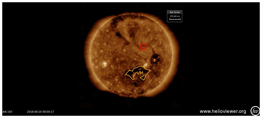
Figure 1Image of the Sun with EUV SDO AIA193 (extreme-ultraviolet NASA Solar Dynamics Observatory Atmospheric Imaging Assembly 19.3 nm) imagers at the time of the filament eruption. The red circle marks the position of the filament eruption associated with the CME; the yellow contour marks the position of the coronal hole. Image created using the ESA- and NASA-funded Helioviewer Project.
The most probable source for the CME is a filament eruption that was observed on 20 August 2018 at t0=08:00 UT at heliographic coordinates on the solar surface (red circle in Fig. 1). The filament ejection was recorded by SDO AIA (NASA Solar Dynamics Observatory Atmospheric Imaging Assembly; Pesnell et al., 2019; Lemen et al., 2011) imagers. Considering the relative positions of STEREO-A at the moment of the CME lift-off, the source on the Sun, the information provided by the CDAW (Coordinated Data Analysis Workshop) catalogue of CMEs and the hypothesis of radial propagation, we can de-project the CME velocity and estimate its radial velocity at about 10 RSun as km s−1. In this respect, we report that the derived radial velocity is lower than the median of the CME speed distribution (Yurchyshyn et al., 2005) and confirms that CMEs associated with filament eruption tend to be slower than those associated with flares (e.g. Moon et al., 2002).
We also note that, at the time of lift-off, a sizable coronal hole (yellow contour in Fig. 1) was present at heliographic coordinates that would generate a fast solar wind stream that could affect the CME propagation. Figure 2 shows the ICME detection by WIND (Lepping et al., 1995), DSCOVR (Burt and Smith, 2012) and ACE (Stone et al., 1998) spacecraft located approximately at the L1 point. An interplanetary (IP) shock passed the three spacecrafts respectively at ∼05:37, ∼05:42 and ∼05:43 UT on 24 August 2018. This IP shock was characterized by a small variation of the solar wind (SW) density ( cm−3, cm−3 and cm−3), velocity (ΔvSW,W≈18 km s−1, ΔvSW,D≈16 km s−1 and ΔvSW,A≈16 km s−1), dynamic pressure (ΔPSW,W≈0.9 nPa, ΔPSW,D≈0.9 nPa and nPa) and interplanetary magnetic field (IMF) strength ( nT, nT and nT). In agreement with the Rankine–Hugoniot conditions, the shock normal for the three spacecrafts was oriented at and , and , and and (solar ecliptic coordinate system). The estimated shock speeds were respectively km s−1, km s−1 and km s−1. Therefore, the predicted time of the impact of the IP shock onto the magnetosphere was at 06:14 UT (32 min after DSCOVR observations). The predicted location of the shock impact at the magnetopause, assuming a planar propagation, was at 07:00 (±00:15) LT (i.e. on the morning side of the magnetopause), corresponding, in the ecliptic plane, to and (GSE is the geocentric solar ecliptic reference system and RE is Earth's radius; Fig. 2g).
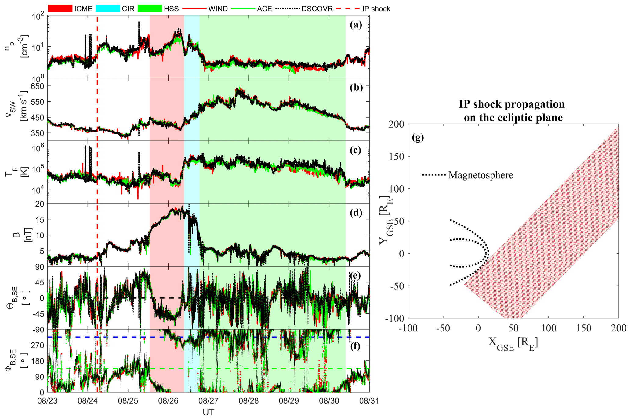
Figure 2Solar wind parameters observed by WIND (red), ACE (green) and DSCOVR (black) spacecraft at L1: (a) proton density; (b) velocity, (c) proton temperature, (d) IMF intensity and (e–f) IMF orientation (ΘSE and ΦSE, respectively) in the SE coordinate system. The vertical horizontal green and blue lines in (f) represent the expected orientation of the Parker spiral at L1. The red dashed line indicates an interplanetary shock as observed on 24 August at ∼05:43 UT (not related to the magnetic cloud structure). The red shaded region identifies the ICME. The cyan and green shaded regions shows the CIR and the HSS, respectively. (g) Interplanetary shock propagation in the ecliptic plane. Please note that the format of the date on the x axis of (a–f) is month/day.
We note that, in principle, the creation of the shock is not incompatible with a slow CME, since the shock can be created by the expansion of the CME as it equalizes its pressure with the interplanetary plasma. Nevertheless, this shock advanced the ICME by more than 30 h. Considering this long time separation, in our opinion this IP shock was not generated by the ICME under analysis.
The 20 August ICME included a significant magnetic cloud, observed at Earth's orbit between 25 August at ∼12:15 UT and 26 August at ∼10:00 UT, whose boundaries are determined (Burlaga et al., 1981) according to the magnetic field behaviour conjoint with the temperature, the velocity and the density of protons, as depicted in Fig. 2: the plasma temperature decreases from K to K; the total magnetic field increases to 16 nT, remaining there for approximately 12 h; the magnetic field smoothly rotated, leading to a pronounced and prolonged southward orientation (beginning at ∼14:30 UT on 25 August) for approximately 22 h and the solar wind speed fluctuated between ∼450 and ∼370 km s−1. A co-rotating interaction region (CIR) followed on 26 August, with the solar wind plasma showing a velocity (temperature) increase at ∼10:00 UT from ∼370 km s−1 ( K) to near ∼550 km s−1 ( K) at ∼12:20 UT and a density increase from ∼11 to ∼30 cm−3, as the solar wind stream was transitioning into a negative-polarity high-speed stream (HSS).
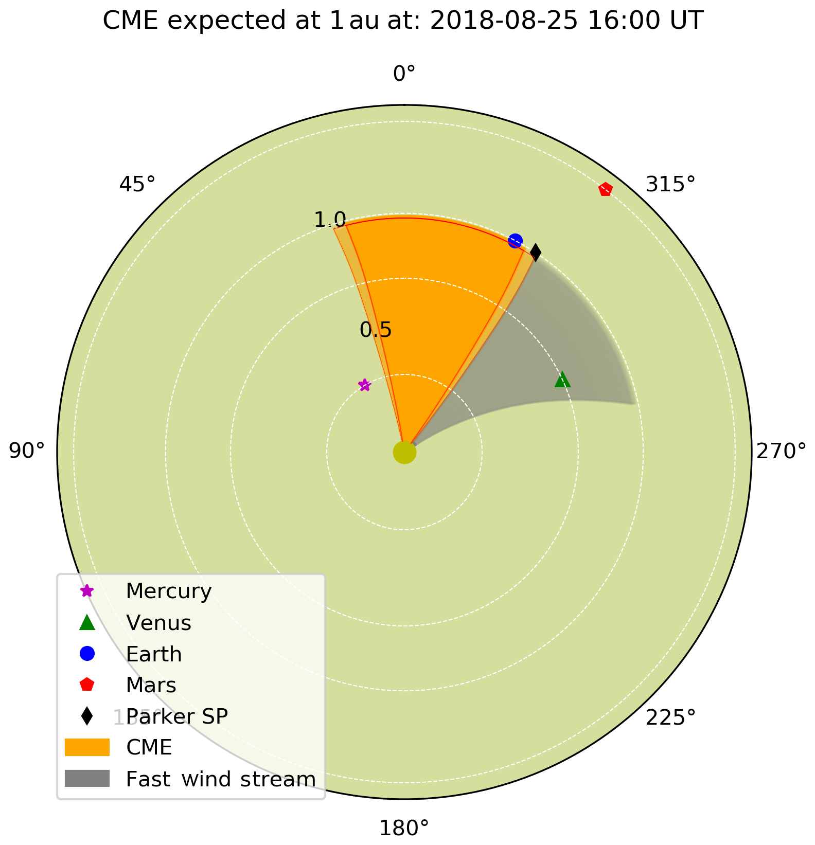
Figure 3Scheme for the propagation of the CME in the inner heliosphere. The positions of the inner planets and Parker Solar Probe (Parker SP) at the time of the ICME arrival at 1 au are represented by coloured symbols. The ICME trajectory computed by the P-DBM model is represented by the orange-shaded area. The lighter-orange areas represent the 1σ uncertainty about the ICME trajectory from the 10 000 different model runs. The grey-shaded area represents instead the fast solar wind stream.
2.2 A model for the propagation of the ICME
To describe the ICME propagation in the heliosphere, we used the P-DBM (Napoletano et al., 2018; Del Moro et al., 2019) model. Considering the presence of the coronal hole (CH) on the Sun at the time of the CME lift-off and the CIR observations of in situ data, we proposed the following scenario, where
-
the ICME propagation is longitudinally deflected by its interaction with the solar wind, as in Eq. (8) of Isavnin et al. (2013);
-
the ICME is later overtaken by the fast solar wind stream from the identified CH at a distance rMix;
-
rMix is computed considering the time for the CH to rotate in the appropriate direction plus the time for the stream to catch up with the ICME.
Applying the same philosophy behind the P-DBM, the longitude of the fast wind stream, generated by the CH, has been associated with a 2.5∘ error with a Gaussian distribution.
From 10 000 runs of this model, the most probable result are that the ICME arrival time and velocity at 1 au are 25 August 2018 at t1 au=16:00 UT (±9 h) and km s−1, respectively, and the fast solar wind stream interacts with the ICME beyond au. These values agree nicely with estimates of the actual arrival characteristics of the ICME as derived in the previous section.
As discussed in Richardson (2018), a CIR would form by the interaction of an HSS with the preceding slower (in this case) ICME. Approximately 1 d later than t1 au, the rotation of the Sun brings the CIR to sweep over Earth's position, followed by an HSS. Last, this model predicts that the ICME that hit Earth would instead miss Mars and possibly also the Parker Solar Probe (PSP), which had been recently launched (Fox et al., 2016). While no data is available for the PSP at that date, no solar particle event was actually detected in the following days by the instrumentation on board MAVEN (Mars Atmosphere and Volatile Evolution; Jakosky et al., 2015). A graphical representation of this result is shown in Fig. 3, where the position of the inner planets and of the Parker Solar Probe at t1 au are represented by coloured symbols. The orange area represents the trajectory of the ICME, with lighter orange areas representing the 1σ uncertainty about its trajectory from the 10 000 different model runs. The grey area represents the part of the inner heliosphere affected by the HSS at t1 au.
A complete and accurate knowledge of the magnetospheric–ionospheric coupling and of its dynamics in response to the changes of the interplanetary medium conditions is critical to many aspects of space weather. It is, indeed, well-known that the changes of the IMF and of the solar wind features, in terms of magnetic field orientation, plasma density, velocity, etc., are capable of generating a fast increase of the magnetospheric–ionospheric current intensities which manifests in multiscale and rapid fluctuations of the ground-based magnetic field. The response of the magnetosphere–ionosphere system to interplanetary changes is however the consequence of both directly driven, i.e. large-scale plasma convection enhancement, and triggered-internal phenomena, such as loading–unloading mechanisms, sporadic plasma energizations in the magnetotail and bursty-bulk flows (Milan, 2017). The response of such a system is strongly dependent on the magnetospheric plasma internal state, with a specific emphasis on the magnetotail central plasma sheet status. The result of the interplay between internal dynamics and directly driven processes has very complex dynamics, showing scale-invariant features typical of non-equilibrium critical phenomena (Consolini et al., 1996, 2018; Consolini, 1997, 2002; Consolini and De Michelis, 1998; Lui et al., 2000; Sitnov et al., 2001; Uritsky and Pudovkin, 1998; Uritsky et al., 2002). In a series of recent papers (Alberti et al., 2017, 2018) the existence of a separation of timescales between directly driven and triggered internal timescales in the response of Earth's magnetosphere–ionosphere current systems as estimated by means of geomagnetic indices in the course of magnetic storms and substorms has been clearly shown. This separation of timescales is one of the fingerprints of the complex character of the geomagnetic response, which makes it very difficult to get a reliable forecast of its short-timescale dynamics.
In this section, we investigate the magnetospheric–ionospheric response during the August 2018 geomagnetic storm. On one hand, the magnetosphere accumulates energy from the solar wind and dissipates it through geomagnetic storms, driving large electrical currents. On the other hand, these currents close down into the ionosphere, producing large-scale magnetic disturbances, such as the auroral electrojets, DP-2 current system, prompt penetrating electric field and so on (Piersanti et al., 2017; Pezzopane et al., 2019, and references therein). Some of these features and phenomena will be discussed in the next sections for the investigated August 2018 geomagnetic storm.
3.1 Magnetosphere
Figure 4a shows the response of the magnetosphere to the front boundary of the magnetic cloud. According to the Shue et al. (1998) model, the magnetopause nose moves inward up to ∼7.1 RE. Indeed, the shape of the magnetospheric field lines before (black lines) and soon after (red lines) the arrival of the magnetic cloud, evaluated by means of the TS04 model (Tsyganenko and Sitnov, 2005), shows large field erosion. Correspondingly, GOES 14 (Geostationary Operational Environmental Satellite; panels b, d and f) and GOES 15 (panels c, e and g) show, on 25 August at ∼06:30 UT, a strong compression ( nT and nT) of the magnetic field coupled with a stretching of the magnetotail field lines, due to the southward switching of the IMF orientation (as already found by Villante and Piersanti, 2011; Piersanti and Villante, 2016; Piersanti et al., 2017). This situation completely changes between 25 August at 13:55 UT and 26 August at 10:25 UT, corresponding to the lowest values of the southward IMF (Bz,IMF) in the magnetic cloud. In fact, both GOES 14 and GOES 15 show a strong decrease of Bz (panels f and g), interpreted in terms of magnetic reconnection between the magnetospheric field and the strong Bz,IMF ( nT) observed in the corresponding interval (Piersanti et al., 2017, and references therein). Interestingly, both GOES satellites show a huge increase of the Bx component (panels b and c) and a negative and then positive variation in the By component (panels d and e). This behaviour is the signature of a strong stretching and twisting of the magnetospheric field lines during the main phase of the geomagnetic storm (Piersanti et al., 2012, 2017). This scenario is confirmed by a modified Tsyganenko and Sitnov (TS04∗; 2005) model indicated by red dashed lines in Fig. 4. Model changes include the magnetopause and the ring current alone, during the main phase, and the concurring contribution of both the ring and the tail currents, during the recovery phase. The TS04∗ model represents very well the magnetospheric observations at geosynchronous orbit, with an average correlation coefficient (r) for the three magnetic field components: r=0.92 for GOES 14 and r=0.75 for GOES 15.
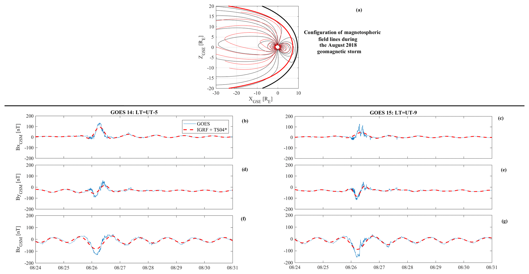
Figure 4(a) Magnetospheric field lines configurations as predicted by the TS04 model before (black lines) and after (red lines) the passage of the front boundary of the magnetic cloud. (b, d, f) Magnetospheric field observations along XGSM (b), YGSM (d) and ZGSM (geocentric solar magnetospheric coordinates) (f) at GOES 14 (LT = UT − 5) geosynchronous orbit. (c, e, f) Magnetospheric field observations along XGSM (b), YGSM (d) and ZGSM (f) at GOES 15 (LT = UT − 5) geosynchronous orbit. Red dashed lines represent the IGRF + TS04∗ (IGRF being the International Geomagnetic Reference Field) model prevision. Please note that the format of the date on the x axis is month/day.
Figure 5a–c show the CSES (China Seismo-Electromagnetic Satellite) satellite (Shen et al., 2017) magnetic observations (Zhou et al., 2019) along the north–south (BN; panel a), east–west (BE; panel b) and vertical (BC; panel c) components after removing the internal and crustal contributions to Earth's magnetic field (using the CHAOS-6 model; Finlay et al., 2016).
CSES is a Chinese satellite launched on 11 February 2018 hosting, among others, a fluxgate magnetometer, an absolute scalar magnetometer, two Langmuir probes and two particle detectors. The satellite orbits at about 500 km of altitude (low-Earth orbit – LEO) in a quasi-polar Sun-synchronous orbit and passes at about 14 and 2 local time (LT) in its ascending and descending orbits, respectively.
As expected (Villante and Piersanti, 2011), the greatest variations are observed along the horizontal components, where both the magnetospheric and ionospheric currents play a key role.
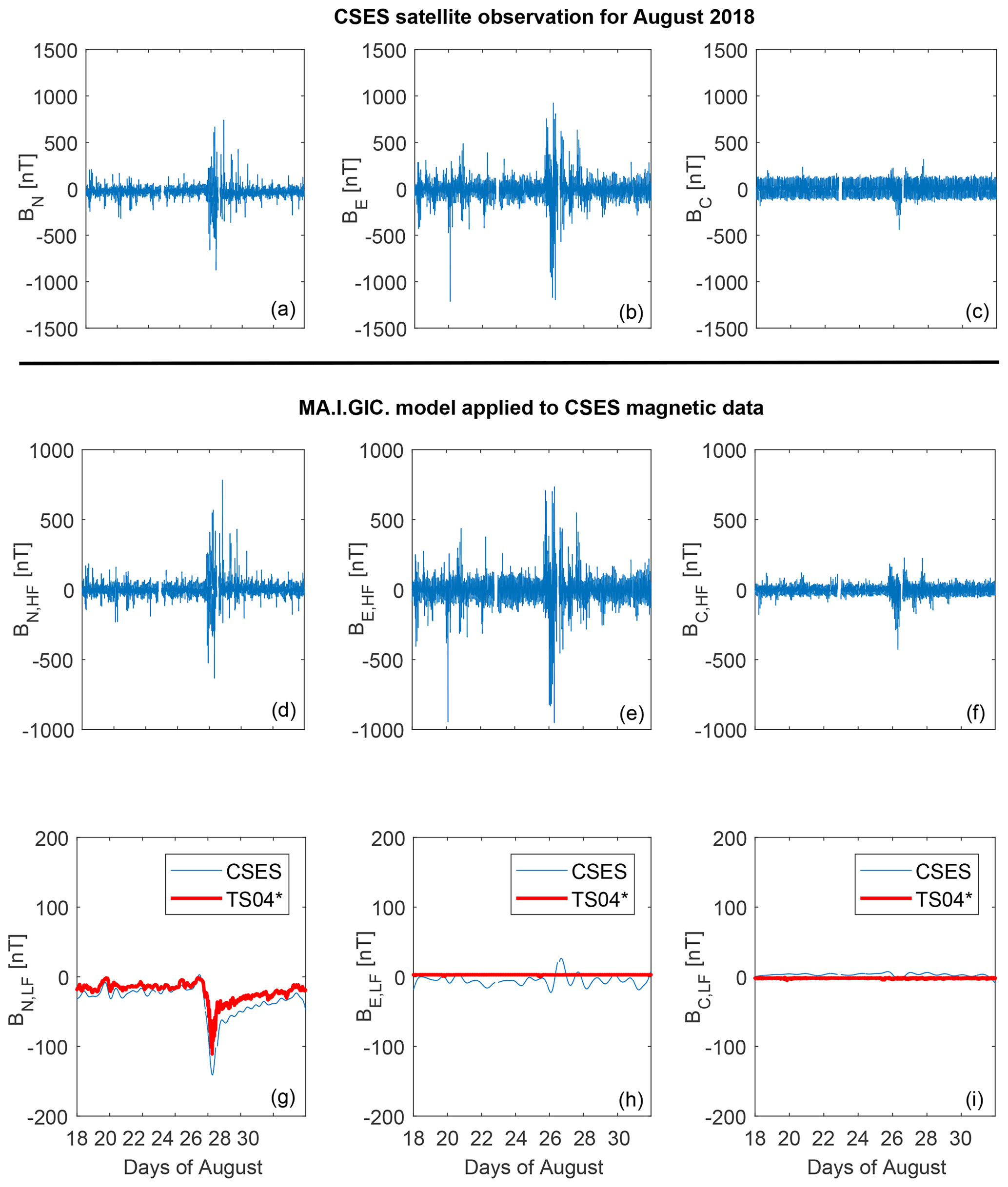
Figure 5Magnetic field observations at the CSES orbit along geographic north–south (a), east–west (b) and vertical (c). MA.I.GIC. model applied to CSES magnetic data: panels (d–f) show the high-frequency timescales (∼25 µHz < f mHz; f being the frequency) for the three components of the observed field; panels (g–i) show the low-frequency timescales (∼2.3 µHz < f µHz) for the three components of the observed field. Red lines represent the TS04∗ model previsions along the CSES orbit.
In order to quantify both the magnetospheric- and ionospheric-origin contributions at the CSES orbit, we applied the MA.I.GIC. (Magnetosphere‐-Ionosphere‐-Ground‐Induced Current) model (Piersanti et al., 2019) to discriminate between different timescale contributions in a time series. The results obtained are shown in Fig. 5d–i. Figure 5d–f and g–i report high- (∼25 µHz < f mHz; f being the frequency) and low-frequency (∼2.3 µHz < f µHz) component observations, respectively. The low-frequency behaviour shows a strong and rapid decrease along the north–south direction during the main phase of the geomagnetic storm and a long-lasting increase during the recovery phase. On the other hand, BE,LF shows a negative and then positive variation during the main and the recovery phase, respectively. BC,LF is characterized by negligible variations. This behaviour is consistent with magnetospheric-origin field variations induced by the action of both the symmetric part of the ring current and tail current along BN,LF and of the asymmetric part of the ring current along BE,LF (Piersanti et al., 2017). It is confirmed by the comparison between the CSES magnetospheric-origin contribution and the TS04∗ model (red lines in Fig. 5d–i), in which we considered both the magnetopause and ring current alone during the main phase, and both the ring current and tail current alone during the recovery phase. It can be easily seen that TS04∗ represents the variations along BN,LF well, while it is not able to reproduce the BE,LF variations. This would suggest that the partial ring current field (with the effect of the field-aligned currents associated with the local-time asymmetry of the azimuthal near-equatorial current), which is not included in the TS04 model, plays a relevant role.
The high-frequency components show large variations along both BN,HF and BE,HF. This behaviour is consistent with the contributions due to the variations of the ionospheric current systems and to the magnetospheric–ionospheric coupling processes. In fact, the huge positive and then negative variations observed during the main phase along both the horizontal components can be imputable to the loading–unloading process between the magnetosphere and the ionosphere (Consolini and De Michelis, 2005; Piersanti et al., 2017). On the other hand, the variations observed during the recovery phase, which are positive on average, can be due to the ionospheric DP-2 current system (Villante and Piersanti, 2011; Piersanti and Villante, 2016; Piersanti et al., 2017).
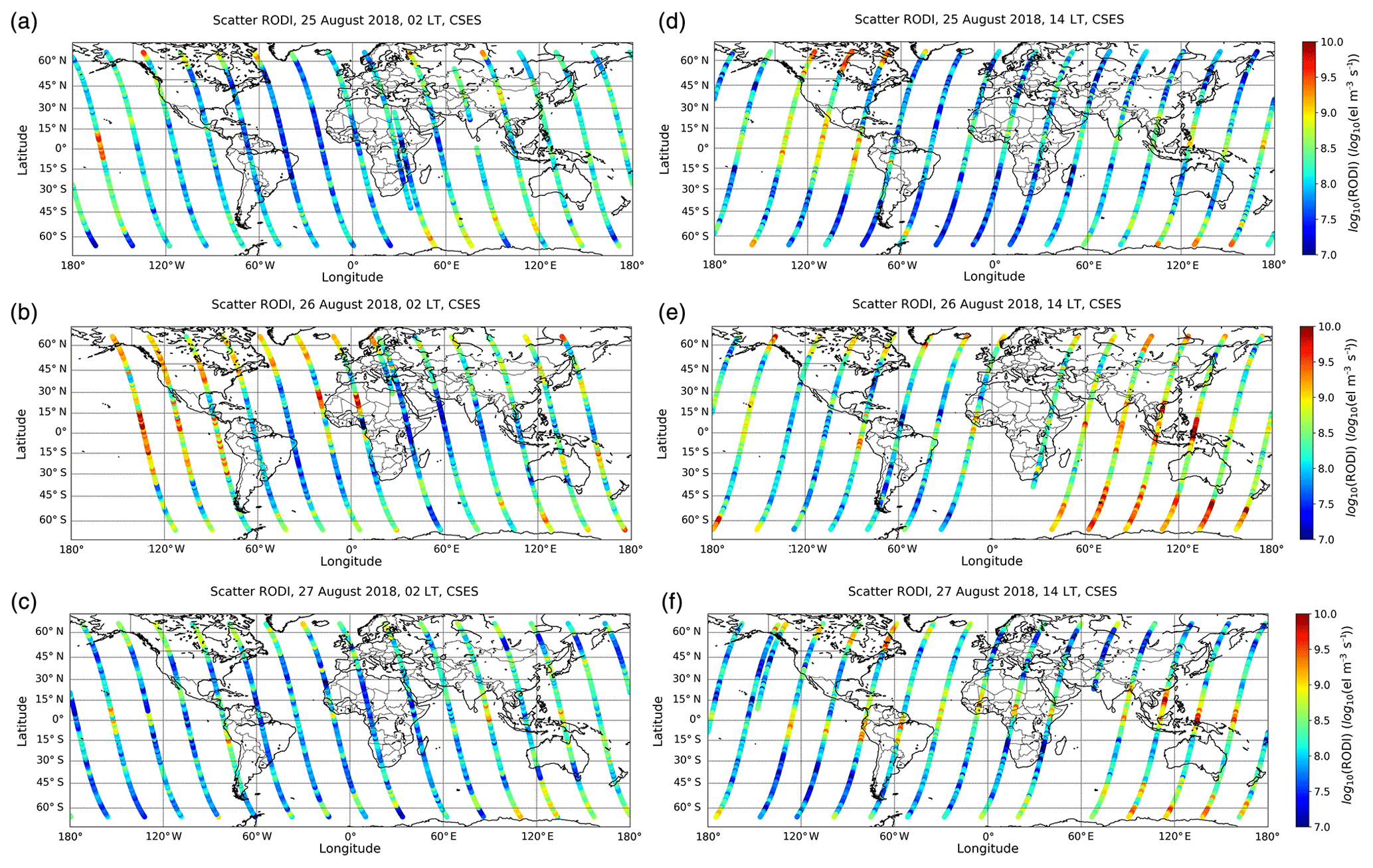
Figure 6RODI values calculated on the basis of electron density values from CSES for 25–27 August 2018. Scale is logarithmic. Coordinates are geographical. Panels (a–c) show nighttime semi-orbits (ascending), while panels (d–f) show daytime semi-orbits (descending). Time increases leftward. On the y axis, el stands for electrons.
3.2 Ionospheric response
The ionospheric plasma is often characterized by irregularities and fluctuations in the plasma density, especially during active solar conditions. We evaluated the RODI index, exploiting electron density measurements made by the CSES satellite (Wang et al., 2019).
Figure 6 shows RODI values for 25–27 August 2018, in which nighttime semi-orbits (around 02:00 LT) are shown separately from daytime semi-orbits (around 14:00 LT).
Significant high values of RODI, spreading all over the meridian during the main phase of the storm (25 and 26 August 2018, especially the latter), for both nighttime and daytime, are clearly seen, while on 27 August 2018, the RODI index comes back to lower values, even though some significant values of RODI are still visible in the Asian–Australian longitude sector at equatorial latitudes. This behaviour can be explained in terms of the presence, during the main phase, of ionospheric irregularities, especially at auroral and low latitudes. To understand whether this significant increase of irregularities could have caused space weather effects on navigation systems, we have considered vertical-total-electron-content (vTEC) data measured by Swarm satellites (Friis-Christensen et al., 2006, 2008) to look for some loss of lock on GPS (Global Positioning System; Jin and Oksavik, 2018, and references therein). As recommended in the Swarm Level 2 (L2) TEC product description (available at https://earth.esa.int/documents/10174/1514862/Swarm_Level-2_TEC_Product_Description, last access: 8 June 2020), only vTEC data with corresponding elevation angles have been taken into account, as these are considered to be more reliable. We have considered vTEC data recorded on 25 and 26 August 2018 by each of the three satellites (A, B and C) of the Swarm constellation and corresponding to each PRN (pseudo-random-noise) satellite in view. No loss of lock has been found, contrary to what happened, for instance, during the well-known and much more intense (i.e. Dst – Disturbed Storm Time index – minimum value reached of −230 nT) St Patrick's Day storm that occurred on 17 March 2015 (Jin and Oksavik, 2018; De Michelis et al., 2016; Pignalberi et al., 2016), where vTEC measurements highlighted many losses of lock (figures not shown). The fact that no loss of lock has been found during the August geomagnetic storm means that the event was weak in terms of space weather effects on navigation systems.
This fact is also supported by Fig. 7, where ROTI (rate of change of TEC index; ROTI is calculated as RODI but considering TEC values in place of electron density values, for a defined GPS satellite in view) values from Swarm A are shown for PRN 8 on 26 August 2018 and for PRN 15 on 17 March 2015. It is clear, from this figure, that a loss of lock occurs when ROTI saturates, a feature that rarely happens on 26 August 2018 and more in general during the entire period under analysis.
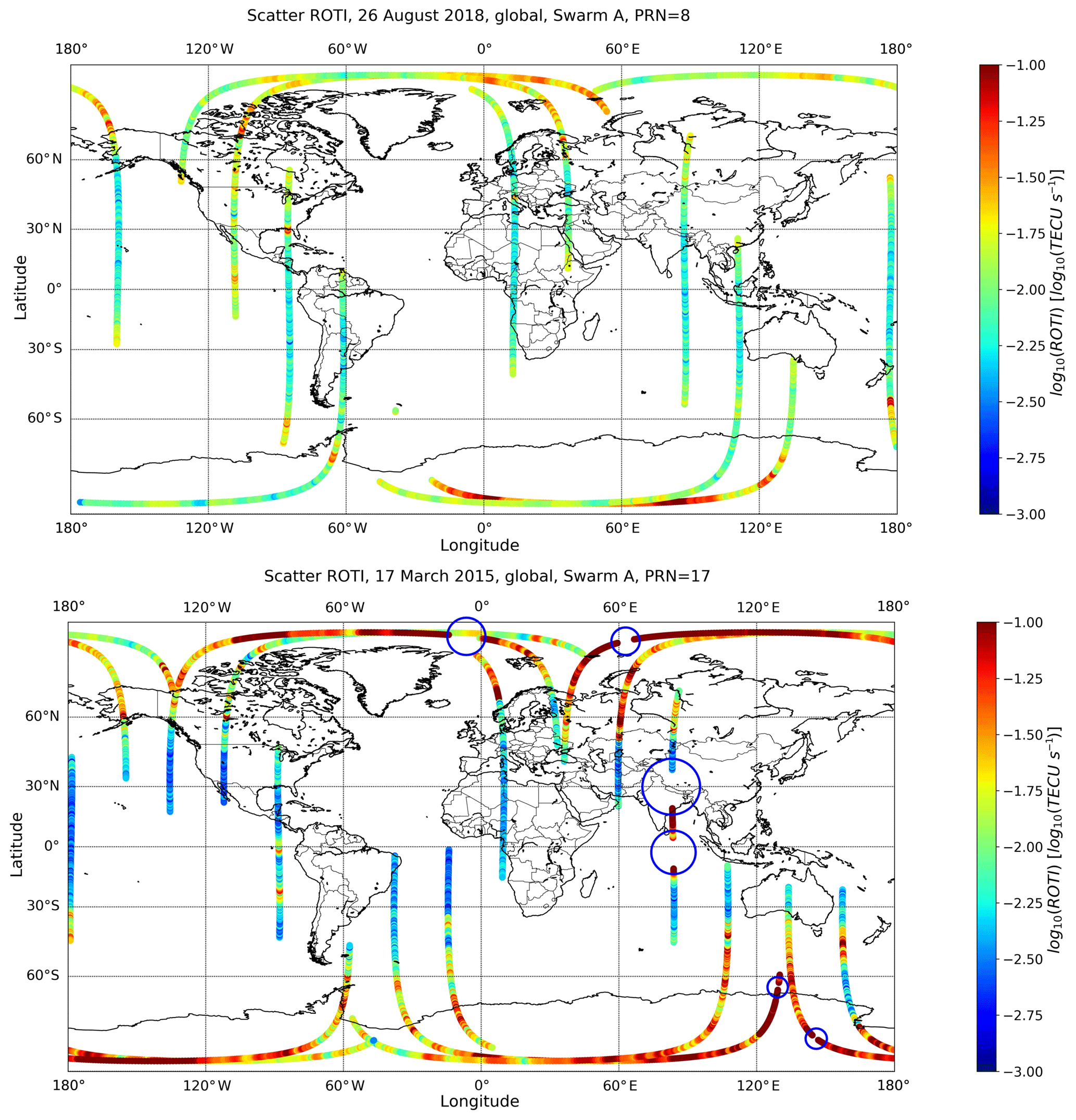
Figure 7ROTI values from Swarm A calculated for PRN 8 on 26 August 2018 and for PRN 17 on 17 March 2015. Losses of lock visible in the figure, highlighted by blue circles, correspond to parts of the trace where ROTI saturates. 1 TECU (total electron content unit) =1016 el m−2.
Space weather predictions and geomagnetic storms intensities are normally measured on the basis of well-known geomagnetic indices. Anyway, as these indices are evaluated using ground observations (typically via magnetometers), it is crucial to improve the knowledge of the effect of each magnetospheric and ionospheric current at ground level. In this section, we focused on the ground magnetic response in terms of magnetospheric and ionospheric currents and on the effects that those currents generated on Earth's surface. GICs are one of the main ground effects of space weather events driven by solar activity (Pulkkinen, 2015; Pulkkinen et al., 2017; Carter et al., 2016; Piersanti et al., 2019). Since GICs represent the end of the space weather chain extending from the Sun to Earth's surface, to complete the description of 25 August 2018 geomagnetic storm, an estimation of the amplitude of geomagnetically induced currents and of the associated risk level, to which power grids have been exposed during this storm, is also presented.
4.1 Geomagnetic field response
To analyse the magnetic effects at ground level during the geomagnetic storm, we selected 83 magnetic observatories from the INTERMAGNET magnetometer array network. INTERMAGNET is a consortium of observatories and operating institutes that guarantees a common standard of data released to the scientific community, thus making it possible to compare the measurements carried out at different observation points. The distribution of the selected observatories is reported in Fig. 8 and covers the geographic latitudes between −80 and 80∘, providing a continuous sampling of the geomagnetic field. Although INTERMAGNET provides geomagnetic data with a time resolution down to 1 s, for our purpose a time resolution of 1 min was sufficient. We have considered the horizontal magnetic field component (H) and focused our analysis on a period of 7 d (from 23 to 29 August), during which the storm occurred. The selected period allows us to follow the evolution of the magnetic disturbance recorded at ground level, during the geomagnetic storm. Moreover, we use the model of Thomas and Shepherd (2018) based on the Super Dual Auroral Radar Network (SuperDARN) to analyse the ionospheric convection during the same period. SuperDARN is an international network of more than 35 high-frequency (HF) radars which has been implemented for the study of the ionosphere and upper atmosphere at sub-auroral, auroral and polar-cap latitudes in both the Northern Hemisphere and Southern Hemisphere (Chisham et al., 2007; Nishitani et al., 2019).
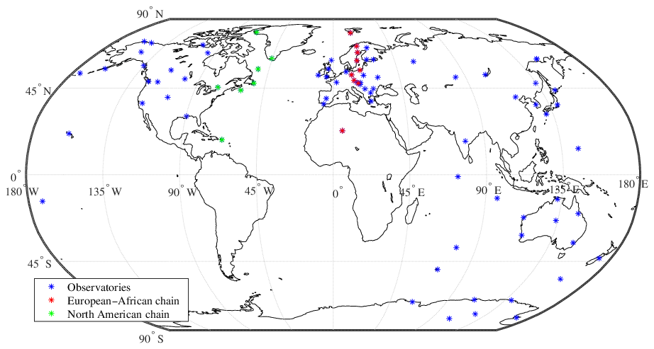
Figure 8Geographical positions of the selected 83 INTERMAGNET geomagnetic observatories (blue stars). Red and green stars identify European–African and North American chains which are almost longitudinal, respectively, selected for the GIC analysis. The map is in geographic coordinates.
Figure 9 shows the daily distributions of the intensity of the horizontal magnetic field component obtained considering data recorded simultaneously by the selected magnetic observatories during the analysed period. The figure reports on the left, the values of the SYM-H index (Iyemori, 1990; Menvielle, 2011), which can be used to monitor the geomagnetic activity and more in detail the ring current intensity during the geomagnetic storm; in the middle, daily polar-view maps of the horizontal field magnitude in the Northern Hemisphere and of the ionospheric convection patterns derived from the model of Thomas and Shepherd (2018) based on SuperDARN observations; and on the right, the cylindrical projection view of the same magnetic field component. Data are reported in geomagnetic latitude and magnetic local time (MLT, Baker, 1989).
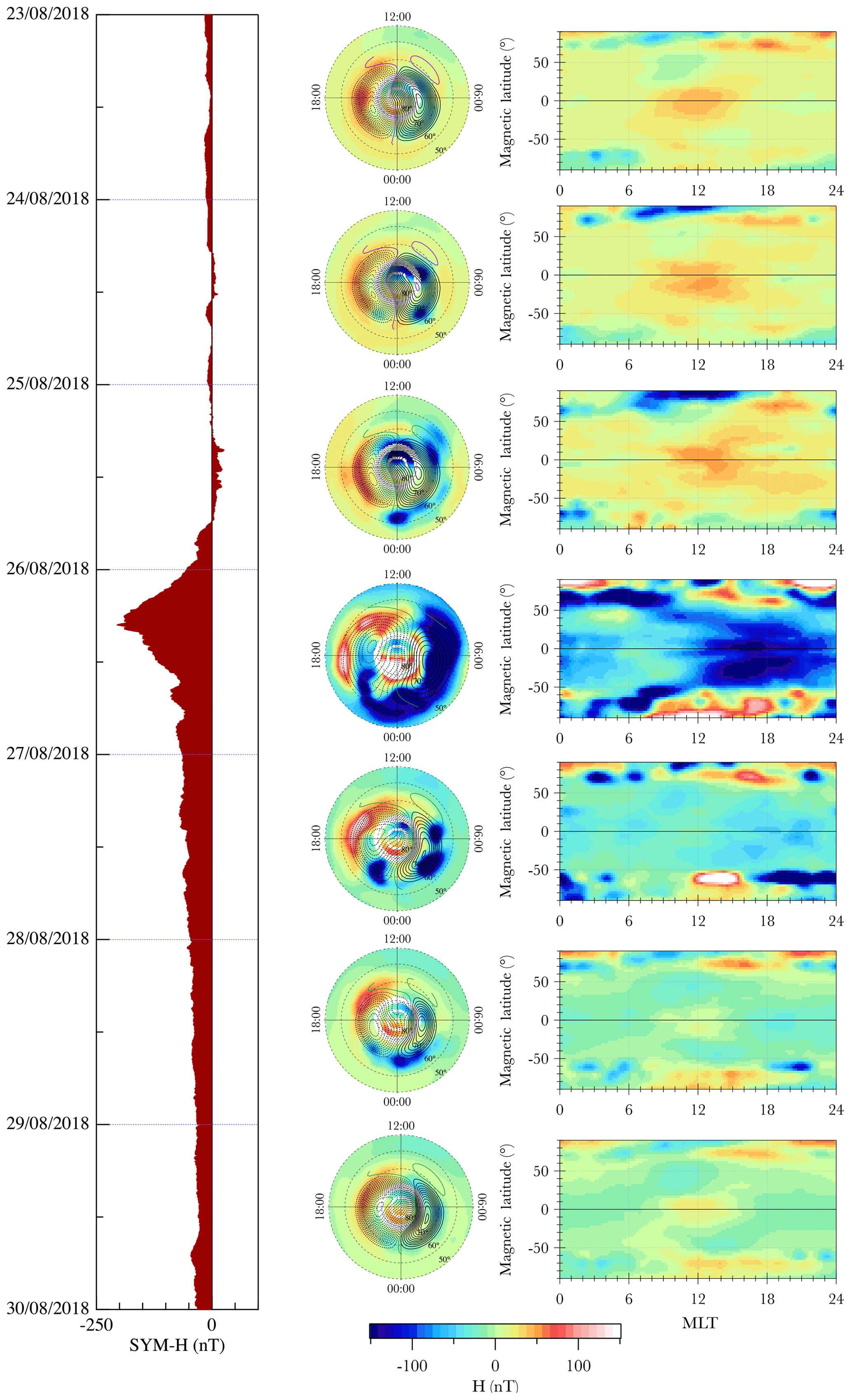
Figure 9On the left is the evolution of the SYM-H index. In the middle column, daily polar-view maps of the horizontal field magnitude in the Northern Hemisphere. The convection patterns derived from the SuperDARN-based model of Thomas and Shepherd (2018) are overplotted on the horizontal field magnitude. In the right column, the worldwide view of the same magnetic field component. Data are reported in geomagnetic latitude and MLT, referring to a period of 7 d from 23 to 29 August 2018.
Of particular interest is the analysis of the effects of the ionospheric and magnetospheric currents on the geomagnetic field. For this reason, we have removed the main field from the data and considered only the magnetic fields generated by the electric currents in the ionosphere and magnetosphere (i.e. the so-called magnetic field of external origin). For this purpose, for each ground station, we removed the internal and the crustal origin fields as modelled by CHAOS-6 (Finlay et al., 2016). Thus, the values of the horizontal field magnitude reported in Fig. 9 describe the magnetic field perturbations at ground level due to external sources. The main contributions to this external field, producing relevant signatures in magnetic field observations, are the polar ionospheric currents, such as the auroral electrojets, and the magnetospheric currents, such as the Chapman–Ferraro currents and (in particular) the magnetospheric ring current (Rishbeth and Garriot, 1969; Hargreaves, 1992). These current systems are almost always present even during geomagnetic quiet periods but show a significant variability during the disturbed periods (De Michelis et al., 1997). The maps reported in Fig. 9 show the effect due to the eastward and westward auroral electrojets. These two polar current systems, which are the most prominent currents at auroral latitudes, produce at ground level a magnetic field perturbation that is characterized by a positive excursion of the horizontal field magnitude in the case of the eastward electrojet, flowing in the afternoon sector, and a negative one in the case of the westward electrojet, flowing through the morning and midnight sector (De Michelis et al., 1999). It can be especially seen from the data reported in the polar-view maps (central column in Fig. 9). We noticed that these currents are always present but that their intensities increase during the main phase of the geomagnetic storm (Ganushkina et al., 2018). Even their spatial distribution changes. Indeed, the magnetic disturbance, associated with these electric currents, tends to shift towards lower-latitudinal values drastically during the geomagnetic storm. On 26 August the westward electrojet is extremely intense, and around midnight the effect at ground level due to the substorm electrojet current is recognizable, too. The associated disturbance fields cover the geomagnetic latitudes from 50 to 75∘ on the nightside. Looking at the ionospheric convection as derived from the statistical model of Thomas and Shepherd (2018) and considering that mean daily values of the IMF and solar wind velocity have been used as input to the model, the convection patterns match the expansion to lower latitudes observed in the magnetic disturbance evolution during the extreme driving conditions (ESW≥4.0 mV m−1) that characterize the period under study after the southward rotation of the IMF. In fact, the convection maps computed from the SuperDARN measurements at 2 min resolution (not shown) also show that the auroral convection zone expands equatorward to 50∘ geomagnetic latitude during the geomagnetic storm. The expansion of the convection pattern is related to the dayside reconnection, forming new open field lines once the IMF turned southward in late 25 August.
The panels on the right column of Fig. 9 show the effect due to the ring current that is responsible for a decrease of the magnetic field intensity at low and mid latitudes, during the development of the geomagnetic storm. As is known, the intensity of the ring current increases during the main phase of a geomagnetic storm because of the injection of energetic particles from the magnetotail in the equatorial plane, and it gradually decays during the recovery phase. The time evolution of the ring current, through the time evolution of its associated disturbance field, is clearly visible in our data. During the main phase of the storm (26 August), the increasing of the ring current flowing in the westward direction produces a strong depression of the horizontal field magnitude, as can be seen by the blue region at mid and low latitudes of the map corresponding to 26 August, on the right-side of Fig. 9. In the days following, the main phase the magnetic field perturbation associated with the ring current is still visible at low and mid latitudes, although its amplitude rapidly decreases. We can conclude that the magnetic field perturbations on the ground due to the arrival of the solar perturbation are clearly recognizable in the recorded data and are well in agreement with what is expected from a theoretical point of view (Piersanti et al., 2017, and references therein).
4.2 Ground magnetic effects
Fluctuations of the geomagnetic field happening during geomagnetic storms or substorms are responsible for an induced geoelectric field at Earth's surface that, in turn, originates GICs that may represent a hazard for the secure and safe operation of electrical power grids and oil and gas pipelines. For instance, for the case of power transmissions, GICs represent a hazard due to their frequency. Indeed, the power spectrum of the originating geoelectric field is dominated by frequencies smaller than 1 Hz, and this makes the GIC a quasi-DC current compared to the 50–60 Hz AC power systems, with the consequence of temporarily or permanently damaging power transformers (Pulkkinen et al., 2017, and references therein).
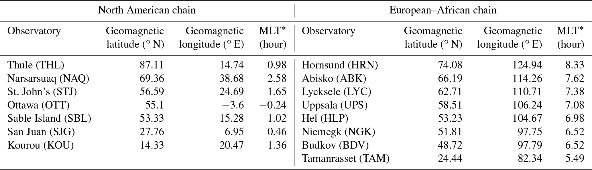
As a proxy of the geoelectric field, and hence of GIC intensity, the GIC index (Marshall et al., 2010) is calculated using the approach proposed by Tozzi et al. (2019). Among the proxies of the geoelectric field resorting to magnetic data only, this index has two main advantages: (1) it represents the geoelectric field better than other commonly used quantities (i.e. dB∕dt or other geomagnetic activity indices), and (2) its values are used to determine the risk level to which power networks are exposed during space weather events (Marshall et al., 2011). Since the components of the geomagnetic field relevant for the induction of the geoelectric field are the horizontal ones, i.e. the northward (X) and eastward (Y) components, the GIC index is calculated for both of them. In particular, GICy and GICx indices are obtained using 1 min of X and Y components, respectively, as observed at the geomagnetic observatories aligned along two latitudinal chains crossing North America and Europe–Africa. These two sets of observatories satisfy the condition to be characterized by geomagnetic longitudes that are spread over a range of around a central longitude. In the case of the North American chain, the central geomagnetic longitude is about 17∘ E, and the observatories used for this chain, indicated by their IAGA (International Association of Geomagnetism and Aeronomy) codes and ordered from high to low geomagnetic latitude, are THL, NAQ, STJ, OTT, SBL, SJG and KOU. The central geomagnetic longitude of the European–African chain is about 105∘ E, and the corresponding observatories, listed as above, are HRN, ABK, LYC, UPS, HLP, NGK, BDV and TAM. Details on the observatories of the two chains can be found in Table 1.
Table 1Details of the geomagnetic observatories used in the study, from left to right, indicate the name and IAGA code of the observatory, geomagnetic latitude, geomagnetic longitude and MLT∗, representing the number of hours to add to 00:00 UT to obtain the MLT location of each observatory.
To have an idea of the maximum GIC intensity produced by the 26 August 2018 geomagnetic storm, we calculated GICx and GICy indices for the geomagnetic observatories of the two chains and then picked out the maximum values reached by both GIC indices from 25 August 2018 at 18:00 UT to 26 August 2018 at 18:00 UT (i.e. the most geomagnetically disturbed conditions) and plotted them as a function of geomagnetic latitude in Fig. 10. The two curves displayed in both panels (a) and (b) of Fig. 10 refer to the North American (red) and to the European–African (blue) observatories chains, respectively. As expected, the latitudinal dependence of the maximum GIC intensity shows an increase with increasing latitude with a steepening of the curve around 60∘ N and then a substantial decrease at the highest latitude, near the geomagnetic pole. This reflects the geometry and the features of the current systems responsible for time variations of the geomagnetic field originating the induced geoelectric field. High latitudes are affected by the effects of the auroral electrojets whose intensity undergo dramatic variations, even increasing up to 4–5 times its quiet time value (Smith et al., 2017). Low and mid latitudes are mainly affected by the ring current that produces variations of the geomagnetic field that are less effective for GICs building up. So, the peaks around 65–75∘ N, well visible in Fig. 10, can be interpreted in terms of the position of the auroral oval and hence of the auroral electrojets flowing. Moreover, as can be observed by Fig. 10, both the European–African and North American chains provide peaks of the GIC indices at different geomagnetic latitudes. In detail, the peak along the European–African chain seem to occur at latitudes smaller than that along the North American chain. Such observations can be explained in terms of the MLT at which the maxima of the GIC indices occur at the observatories of the two chains: around (01:00 ± 01:00) MLT for the European–African chain and around (21:00 ± 01:00) MLT for the North American chain. Indeed, as can be deduced by Fig. 9, especially by looking at the worldwide view of the horizontal field magnitude, the maximum variation of the horizontal component of the geomagnetic field recorded on 26 August around 01:00 MLT occurs at latitudes lower than that observed at 21:00 MLT. The more the auroral oval expands towards lower latitudes, the smaller the latitude where the steepening of the maximum GIC index is. Since, as already mentioned, the advantage to use the GIC index relates to the availability of an associated risk level scale, Fig. 10 also displays coloured dashed lines that indicate the boundaries between adjacent risk levels. This risk level scale has been introduced and defined by Marshall et al. (2011), it consists of four risk levels going from “very low” to “extreme”, each associated with defined ranges of the GICx and GICy indices. This scale is based on a large occurrence of faults or failures of worldwide power grids and represents a probabilistic description of the threat, with the risk level providing the probability to have a fault; detailed information about this scale is given in Marshall et al. (2011). Results shown in Fig. 10 tell that, for the analysed geomagnetic storm and for the same latitudes, power networks located along the European–African chain have been exposed to higher risk levels than those located along the North American chain.
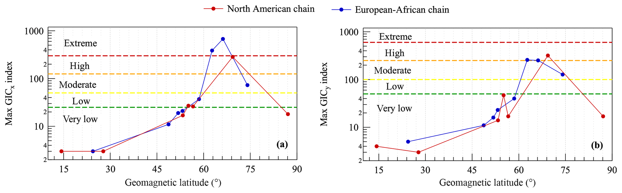
Figure 10Maximum value of the GIC indices that occurred in the time interval from 25 August 2018 at 18:00 UT to 26 August 2018 at 18:00 UT, as observed at the magnetic observatories of both the North American and European–African latitudinal chains. In detail, (a) displays the maximum values of the GICx index, and (b) displays the maximum values of the GICy index. Coloured dashed lines indicate the thresholds between the different risk levels as defined by Marshall et al. (2011).
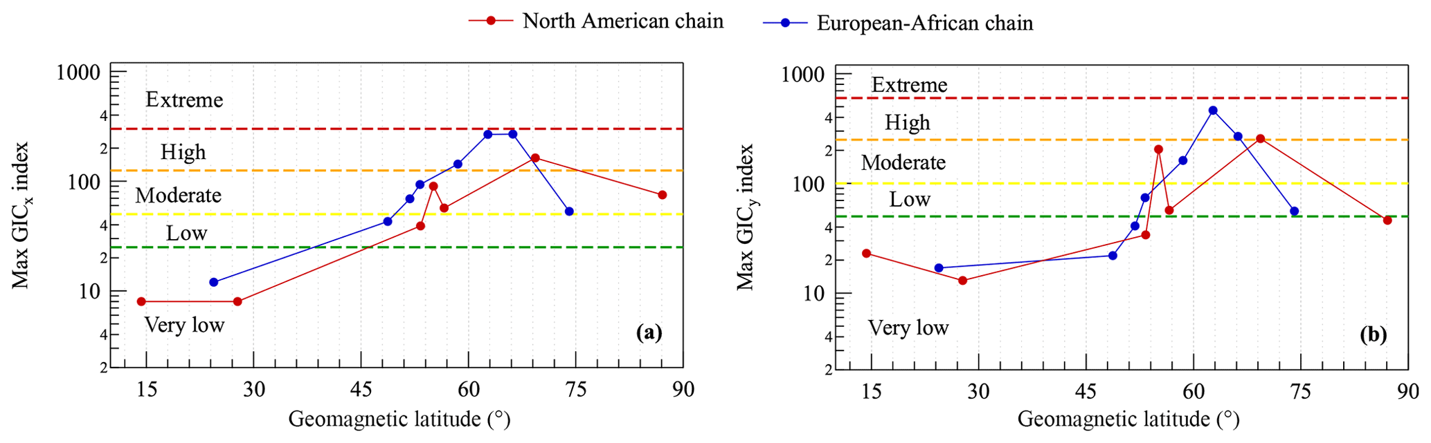
Figure 11Maximum value of the GIC indices that occurred in the time interval from 17 March 2015 at 04:00 UT to 18 March 2015 at 04:00 UT, as observed at the magnetic observatories of both the North American and European–African latitudinal chain. In detail, (a) displays the maximum values of the GICx index, and (b) displays the maximum values of the GICy index. Coloured dashed lines indicate the thresholds between the different risk levels as defined by Marshall et al. (2011)
As in the case of the ionospheric response, we repeated the analysis (same method and observatories), using data recorded during the 2015 St Patrick's Day geomagnetic storm (Fig. 11), in order to have a quantitative comparison of the effects of the two storms. There are evident similarities between Figs. 11 and 10, but some interesting differences can be highlighted. First, although the 2015 St Patrick's Day storm was slightly more intense than the 26 August 2018 geomagnetic storm (minimum values of the SYM-H index of −234 and −206 nT, respectively), its maximum value of the GIC index is lower and occurs mainly on the dayside for both chains of observatories. This difference could be ascribed to the different location of the magnetic cloud impact at the magnetopause: in the morning for the 2018 August storm and on the nose of the magnetopause for the 2015 St Patrick's Day storm. Second, during the St Patrick's Day storm, the southern boundary of the auroral oval experienced a larger equatorward expansion. This can be deduced by the value of the southernmost latitudes exposed to risk levels higher than “moderate”. In the case of the August storm, these are larger than around 60∘ N, while during the St Patrick's Day storm, they decreased to around 45–50∘ N. Last, the maximum values of GIC index at low–mid latitudes are very low for both geomagnetic storms but slightly higher in the case of the St Patrick's Day storm. This suggests a greater participation of other current systems as, for instance, the ring current.
The solar event that has been associated with the 25 August 2018 geomagnetic storm that occurred on 20 August 2018. The most probable source for the CME is a filament eruption observed at 08:00 at heliographic coordinates on the solar surface (Pink post in Fig. 1). The filament ejection has been recorded by SDO EUV imagers.
In order to reconstruct the ICME behaviour in interplanetary space and to link the results from remote-sensing and in situ data, we propagate the CME in the heliosphere in the framework of the P-DBM (Napoletano et al., 2018) model under the hypotheses that the ICME propagation is longitudinally deflected by its interaction with the solar wind and the ICME is later overtaken by a fast solar wind stream from the identified coronal hole at a distance rmix, which is evaluated considering the concurring contribution of both the time for the CH to rotate in the appropriate direction and the time for the stream to catch up with the ICME. The results are an ICME arrival time and velocity at 1 au of 25 August 2018 at 16:00 UT (±9 h) and (440±70) km s−1. The failure to observe an IP shock ahead the CME can be due to a large inclination of the normal of the magnetic cloud structure (Fig. 3). Such a peculiarity, associated with the fact that the CME was slow and weak, made it very hard for L1 SW satellites to detect a true IP shock (Oliveira and Samsonov, 2018). This scenario is confirmed by the solar wind observations at L1. In fact, the ACE, WIND and DSCOVR satellites detected the ICME arrival on 25 August 2018 at ∼12:15 UT. As a consequence of the magnetic cloud arrival, the magnetospheric field lines configuration reveal a large magnetopause erosion from 10 RE to 7.1 RE as both predicted by the TS04 model and observed by the GOES 14 and GOES 15 satellites, caused by the gradual depletion of Bz,IMF. In addition, the magnetosphere is stretched and twisted as a consequence of the action of the magnetopause and the ring current alone between 25 August 2018 at 13:55 UT and 26 August 2018 at 08:15 UT (corresponding to the main phase of the geomagnetic storm, at ground level) and of the concurring contribution of both the ring and the tail currents between 26 August 2018 at 08:15 UT and 31 August 2018 (corresponding to the recovery phase of the geomagnetic storm, at ground level). This scenario is confirmed by the simulation of a modified TS04 model set with the previous magnetospheric current assumptions, which well represents the behaviour of the observations at geosynchronous orbit (red dashed lines in Fig. 4). A similar situation is obtained at LEO orbit on the CSES satellite (Fig. 5), where the magnetospheric-origin field variations (low-frequency contributions) are induced by the action of both the symmetric part of the ring current and tail current along BN,LF and of the asymmetric part of the ring current along BE,LF (Piersanti et al., 2017), as confirmed by the TS04∗ model previsions. Differently from GOES observations, CSES shows also variations at higher frequencies (∼0.025 mHz < f mHz), which are both the ionospheric-current-system and the magnetospheric–ionospheric-coupling-origin contributions. Our interpretation of the huge positive and then negative variations observed during the main phase along both the horizontal components is due to the loading–unloading process between the magnetosphere and the ionosphere (Consolini and De Michelis, 2005; Piersanti et al., 2017). On the other hand, the variations observed during the recovery phase are due to the ionospheric DP-2 current system (Villante and Piersanti, 2011; Piersanti and Villante, 2016; Piersanti et al., 2017).
At ground level, during the main phase, the disturbance fields observed at latitudes between 50 and 75∘, on the night side, are due to the intensification of the westward auroral electrojet. In addition, on 26 August 2018, the pattern of the auroral electrojets are consistent with an ICME impacting on the morning side of the magnetosphere. In fact, as expected (Wang et al., 2010; Piersanti and Villante, 2016; Pilipenko et al., 2018), the greater disturbance for both the westward and eastward electrojets are located around 07:00 LT (central panels of Fig. 9). In addition, it is interesting to note that the large values of the westward electrojet could be due to the concurring contributions of the magnetic cloud and CIR that increase the unloading process from the tail to polar region (Consolini and De Michelis, 2005, and references therein). On the same day, the injection of energetic particles from the magnetotail in the equatorial plane increased the ring current, generating at lower latitudes a strong depression of the horizontal field magnitude on Earth's surface (right panels in Fig. 9). During the recovery phase, we observed a return of the horizontal component of the geomagnetic field to pre-storm values due to the decrease the ring current amplitude (Piersanti et al., 2017).
From an ionospheric point of view, to figure out whether the significant increase of electron density irregularities recorded in terms of RODI, especially during the main phase, affected navigation systems, we estimated the loss of lock from vTEC Swarm data. No loss of lock has been found, which means that the event was weak in terms of space weather effects on navigation systems. This fact is supported by Fig. 7, showing that loss of lock occurs mainly for really high values of ROTI, values which were never recorded during the period under analysis.
The amplitude of the geomagnetically induced currents index (Marshall et al., 2011; Tozzi et al., 2019), evaluated during the August 2018 geomagnetic storm, reached very high values above 60∘ N of geomagnetic latitude. A direct comparison to St Patrick's Day event showed that despite the different storm intensities, the GIC hazard was extreme during the August 2018 event, while only high in the March 2015 event. On the other hand, both storms present very low values of the GIC index at low–mid latitudes, suggesting a greater participation of the ring current system. In any case, it is possible to observe the different impact of this storm at two different MLTs that is in good agreement with the reconstruction of the geomagnetic disturbance as recorded on the ground (see Fig. 9).
The solar event that occurred on 20 August 2018 has been capable of increasing the intensity of the various electric current systems flowing in the magnetosphere and ionosphere and activating a chain of processes which cover a wide range of time and spatial scales and, at the same time, of activating strong interactions between various regions within the solar–terrestrial system. The geomagnetic storm and the magnetospheric substorms that occurred in the days following the solar event are the typical signatures of this chain of processes. The long-lasting reconnection at the dayside magnetopause led to an increase of magnetospheric circulation and to an injection of particles into the inner magnetosphere and more generally provided free energy which was stored in the magnetosphere and led to a worldwide magnetic disturbance. The development of such a disturbance has led to an increase of currents in the ionosphere accompanied by the auroral activity and by a shift equatorward of the auroral electrojets and to the growth of the ring current (i.e. the westward toroidal electric current flowing around Earth on the equatorial plane) accompanied by a worldwide reduction of the horizontal components of the geomagnetic field at low and mid latitudes. Rapid geomagnetic variations induced geoelectric fields on the conducting ground responsible for GICs whose intensity, as expected, varied with geomagnetic latitude (Tozzi et al., 2018, and references therein). The amplitude of these currents, quantified by means of the GIC index, has reached values corresponding to “high” and “extreme” risk levels above 60∘ N of geomagnetic latitude. However, no failures or malfunctioning are reported in the literature. A higher sampling of the different geomagnetic latitudes would have been allowed to more precisely depict GIC variations with latitude.
This storm is one of the few strong geomagnetic storms (G3 class; https://spaceweather.com/, last access: 3 June 2020) that occurred during the current, 24th solar cycle and represents one of those cases which have clearly shown how unpredictable space weather is and how much work is needed to make reliable predictions of the effects that solar events could have on the terrestrial environment. Indeed, the CME emitted by the Sun in the days before the occurrence of the geomagnetic storm showed no features that would suggest the occurrence of important effects in the circumterrestrial environment or at ground level. Indeed, as numerous studied have shown, the magnitude and features of geomagnetic storms depend not only on solar wind plasma parameters and on the values of the IMF but also on their evolution (Piersanti et al., 2017, and references therein). Failing to predict the intensity of the 26 August 2018 storm has meant not being able to correctly estimate its effects on anthropic systems such as satellites, telecommunications, power transmission lines and the safety of airline passengers. This confirms that, despite considerable advances in understanding the drivers of space weather events, there is still room for improvement for their forecasting. It is important to underline that the future capabilities of forecasting if, where and when an event occurs and how intense it will be will depend on our understanding of the physical processes behind the dynamics in near-Earth space (Singer et al., 2013; Pulkkinen, 2015; Piersanti et al., 2019).
As a closing remark, we stress that, from a space weather point of view, this kind of comprehensive analysis plays a key role in better understanding the complexity of the processes occurring in the Sun–Earth system that determines the geoeffectiveness of solar activity manifestations.
To define RODI, it is necessary to calculate the rate of change of the electron density (ROD), defined as
where Ne(t) and Ne(t+δt) are the electron density measured by the Langmuir probe on board the CSES satellite at time t and (t+δt), respectively; δt=3 s, since the CSES Langmuir probe sampling rate is 1∕3 Hz. Electron density values are provided in the form of continuous time series as a function of time; however, missing measurements is a possibility and an issue that has to be taken into account from a computational point of view. Consequently, time and electron density measured values are indexed through an index k running on the whole time series. With this approach, the kth ROD value is calculated as
where is the electron density measured at a specific time tk and is the electron density measured at time tk+1, only when the condition (tk+1 - tk) = δt=3 s is satisfied, i.e. for time-consecutive measurements (according to the Langmuir probe sampling rate). RODI is the standard deviation of ROD values in a running window of Δt. Specifically, to calculate RODI, only ROD values calculated between and are taken into account. Then, RODI at each definite time t is
where ROD(ti) values are ROD values falling inside the window centred at time t and Δt = 30 s wide. N is the number of ROD values in the window, while is the corresponding mean, that is
From a computational point of view, the kth RODI value is calculated as
where RODk+i are ROD values falling inside the window of width (2j+1), with j = 5, centred at index k. To take into account possible missing measurements in the time series, only ROD values satisfying the condition – s are considered. N is the number of ROD values (at most 11) falling in the window, and is the corresponding mean of these N values, that is
Finally, RODI is calculated only when at least six ROD values fall in the window (the half plus one of maximum values inside a window, with δt=3 s and Δt=30 s). In this way, windows which are poorly populated and consequently not statistically reliable, are discarded.
All the data are publicly available at the following websites: SDO data at https://sdo.gsfc.nasa.gov/data/aiahmi/ (NASA SDO/AIA and the HMI science teams, 2020), SOHO data at https://sohowww.nascom.nasa.gov/data/data.html (SOHO, 2020), DSCOVR data at https://www.ngdc.noaa.gov/dscovr (NOAA's National Centers for Environmental Information Data Center, 2020), INTERMAGNET data at https://www.intermagnet.org/ (INTERMAGNET, 2020), CSES satellite data at http://www.leos.ac.cn (CSES, 2020), OMNI data at https://cdaweb.sci.gsfc.nasa.gov/index.html/ (NASA Goddard Space Flight Center, 2020), GOES data at https://www.swpc.noaa.gov/products/goes-magnetometer (NOAA Space weather prediction center, 2020) and Swarm data at https://earth.esa.int/ (SWARM, 2020).
MP managed the paper, analysed the magnetic field data from both satellite and ground observations, and concurred with the discussion of the results. PDM analysed the geomagnetic data and concurred with the discussion of the results. RT performed the GIC analysis and concurred with the discussion of the results. DDM analysed solar data and ran the simulation of the ICME propagation. MP and AP analysed the ionospheric plasma data and evaluated both ROTI and RODI. GC and VQ analysed the magnetospheric field data and concurred with the discussion of the results. SDM analysed the solar wind data. PD validated and processed the CSES data. ML performed the interplanetary analysis. MFM performed the magnetospheric analysis. All authors approved the final version of the paper.
The authors declare that they have no conflict of interest.
This article is part of the special issue “Satellite observations for space weather and geo-hazard”. It is a result of the EGU General Assembly 2019, Vienna, Austria, 7–12 April 2019.
The authors wish to thank both reviewers for their help in evaluating the paper. The results presented in this paper rely on data collected at magnetic observatories. SDO data are supplied courtesy of the NASA SDO AIA and HMI science teams. SOHO data are supplied courtesy of the SOHO MDI and SOHO EIT consortia. SOHO is a project of international cooperation between ESA and NASA. This research has made use of data provided by the Heliophysics Event Knowledgebase. DSCOVR data were obtained from the NOAA's National Centers for Environmental Information (NCEI) data centre. We thank the national institutes that support them and INTERMAGNET for promoting high standards of magnetic observatory practice (https://www.intermagnet.org/, last access: 3 June 2020). This work made use of the data from the CSES mission (http://www.leos.ac.cn/, last access: 3 June 2020), a project funded by the China National Space Administration and China Earthquake Administration in collaboration with the Italian Space Agency and Istituto Nazionale di Fisica Nucleare. The authors kindly acknowledge Natalia Papitashvili and Joe King at the National Space Science Data Center of the Goddard Space Flight Center for permission to use the 1 min OMNI data and the NASA CDAWeb team for making these data available. We acknowledge the use of the NOAA Space Weather Prediction Center for obtaining GOES magnetometer data. The European Space Agency (ESA) is acknowledged for providing the Swarm data. The official Swarm website is http://earth.esa.int/swarm (last access: 3 June 2020). Mirko Piersanti thanks the Italian Space Agency for financial support (contract ASI “LIMADOU scienza” no. 2016-16-H0). This research work is supported by the Italian MIUR-PRIN for the project “Circumterrestrial Environment: Impact of Sun–Earth Interaction”.
This research has been supported by the Italian Space Agency (contract ASI “LIMADOU scienza” no. 2016-16-H0).
This paper was edited by Georgios Balasis and reviewed by two anonymous referees.
Alberti, T., Consolini, G., Lepreti, F., Laurenza, M., Vecchio, A., and Carbone, V.: Timescale separation in the solar wind-magnetosphere coupling during St. Patrick's Day storms in 2013 and 2015, J. Geophys. Res., 122, 4266–4283, https://doi.org/10.1002/2016JA023175, 2017. a
Alberti, T., Consolini, G., De Michelis, P., Laurenza, M., and Marcucci, M. F.: On fast and slow Earth's magnetospheric dynamics during geomagnetic storms: a stochastic Langevin approach, J. Space Weather Space Clim., 8, 56, https://doi.org/10.1051/swsc/2018039, 2018. a
Baker D. N.: Satellite Anomalies due to Space Storms, in: Space Storms and Space Weather Hazards, NATO Science Series, Series II: Mathematics, Physics and Chemistry, edited by: Daglis, I. A., Vol. 48, Springer, Dordrecht, https://doi.org/10.1007/978-94-010-0983-6_11, 2001. a
Baker, K. B. and Wing S.: A new magnetic coordinate system for conjugate studies at high latitudes, J. Geophys. Res., 94, 9139–9143, https://doi.org/10.1029/JA094iA07p09139, 1989. a
Bothmer, V. and Schwenn R.: The interplanetary and solar causes of major geomagnetic storms, J. Geomagn. Geoelectr., 47, 1127–1132, https://doi.org/10.5636/jgg.47.1127, 1995. a
Brueckner, G. E., Howard R. A., Koomen M. J., Korendyke C. M., Michels D. J., Moses J. D., Socker D. G., Dere K. P., Lamy P. L., Llebaria A., and Bout M. V.: The large angle spectroscopic coronagraph (LASCO), Sol. Phys., 162, 357–402, https://doi.org/10.1007/BF00733434, 1995. a
Burlaga, L., Sittler, E., Mariani, F., and Schwenn, A. R.: Magnetic loop behind an interplanetary shock: Voyager, helios, and imp 8 observations, J. Geophys. Res., 86, 6673–6684, 1981. a
Burt, J. and Smith, B.: Deep Space Climate Observatory: The DSCOVR mission, Aerospace Conference 2012 IEEE, Aerospace Conference, IEEE, 1–13, https://doi.org/10.1109/AERO.2012.6187025, 2012. a
Carter, B. A., Yizengaw, E., Pradipta, E., Weygand, J. M., Piersanti, M., Pulkkinen, A., Moldwin, M. B., Norman, R., and Zhang, K.: Geomagnetically induced currents around the world during the 17 March 2015 storm, J. Geophys. Res., 121, 496–507, https://doi.org/10.1002/2016JA023344, 2016. a
Chisham, G., Lester, M., Milan, S., Freeman, M., Bristow, W., Grocott, W. A., McWilliams, K., Ruohoniemi, J., Yeoman, J., Timothy, T., Dyson, P., Greenwald, R., Kikuchi, T., Pinnock, M., Rash, J., Sato, N., Sofko, G., Villain, J. P., and Walker, A.: A decade of the Super Dual Auroral Radar Network (SuperDARN): Scientific achievements, new techniques and future directions, Surv. Geophys., 28, 33–109, https://doi.org/10.1007/s10712-007-9017-8, 2007. a
Consolini, G., Marcucci, M. F., and Candidi, M.: Multifractal Structure of Auroral Electrojet Index Data, Phys. Rev. Lett., 76, 4082–4085, 1996. a
Consolini, G.: Sandpile Cellular Automata and Magnetospheric Dynamics, Proc. of VIII Conv. GIFCO-97, SIF (Bo), 123–126, 1997. a
Consolini, G. and De Michelis, P.: Non-Gaussian Distribution Function of AE-Index Fluctuations, Evidence for Time Intermittency, Geophys. Res. Lett., 25, 4087–4090, 1998. a
Consolini, G.: Self-organized criticality: a new paradigm for the magnetotail dynamics, Fractals, 10, 275–283, 2002. a
Consolini, G. and De Michelis, P.: Local intermittency measure analysis of AE index: The directly driven and unloading component, Geophys. Res. Lett., 32, L05101, https://doi.org/10.1029/2004GL022063, 2005. a, b, c
Consolini, G., Alberti T., and De Michelis, P.: On the Forecast Horizon of Magnetospheric Dynamics: A Scale-to-Scale Approach, J. Geophys. Res., 123, 9065–9077, https://doi.org/10.1029/2018JA025952, 2018. a
CSES: China National Space Administration and China Earthquake Administration website, available at: http://www.leos.ac.cn, last access: last access: 8 June 2020. a
Del Moro, D., Napoletano, G., Forte, R., Giovannelli, L., Pietropaolo, E., and Berrilli, F.: Forecasting the 2018 February 12th CME propagation with the P-DBM model: a fast warning procedure, Ann. Geophys., 62, 4, https://doi.org/10.4401/ag-7750, 2019. a
De Michelis, P., Daglis, I., and Consolini, G.: Average terrestrial ring current derived from AMPTE/CCE‐CHEM measurements, J. Geophys. Res., 102, 14103–14111, https://doi.org/10.1029/96JA03743, 1997. a
De Michelis, P., Daglis, I., and Consolini, G.: An average image of proton plasma pressure and of current systems in the equatorial plane derived from AMPTE/CCE-CHEM measurements, J. Geophys. Res., 104, 28615–28624, https://doi.org/10.1029/1999JA900310, 1999. a
De Michelis, P, Consolini, G., Tozzi, R., and Marcucci, M. F., Observations of high-latitude geomagnetic field fluctuations during St. Patrick's Day storm: Swarm and SuperDARN measurements, Earth Planets Space, 68, 1–16, https://doi.org/10.1186/s40623-016-0476-3, 2016. a
Domingo, V., Fleck, B., and Poland, A. I.: The SOHO mission: an overview, Sol. Phys., 162, 1–2, https://doi.org/10.1007/BF00733425, 1995. a
Finlay, C. C., Olsen, N., Kotsiaros, S., Gillet, N., and Toffer-Clausen, L.: Recent geomagnetic secular variation from Swarm and ground observatories as estimated in the CHAOS-6 geomagnetic field model, Earth Planet Space, 68, 112–130, https://doi.org/10.1186/s40623-016-0486-1, 2016. a, b
Fox, N. J., Velli, M. C., Bale, S. D., Decker, R., Driesman, A., Howard, R. A., Kasper, J. C., Kinnison, J., Kusterer, M., Lario, D., Lockwood, M. K., McComas, D. J., Raouafi, N. E., and Szabo, A.: The Solar Probe Plus mission: Humanity’s first visit to our star, Space Sci. Rev., 204, 1–4, https://doi.org/10.1007/s11214-015-0211-6, 2016. a
Friis-Christensen, E., Lühr, H., and Hulot, G.: Swarm: A constellation to study the Earth’s magnetic field, Earth Planets Space, 58, 351–358, https://doi.org/10.1186/BF03351933, 2006. a
Friis-Christensen, E., Lühr, H., Knudsen, D., and Haagmans, R.: Swarm – An Earth Observation Mission investigating Geospace, Adv. Space Res. 41, 210–216, https://doi.org/10.1016/j.asr.2006.10.008, 2008. a
Ganushkina, N. Y., Liemohn, M. W., and Dubyagin, S.: Current systems in the Earth's magnetosphere, Rev. Geophys., 56, 309–332, https://doi.org/10.1002/2017RG000590, 2018. a
Ginet, G. P.: Space Weather: An Air Force Research Laboratory Perspective, Space Storms and Space Weather Hazards, NATO Science Series, Series II: Mathematics, Physics and Chemistry, edited by: Daglis, I. A., Vol. 38, Springer, Dordrecht, 437–457, https://doi.org/10.1007/978-94-010-0983-6_18, 2001. a
Gonzalez, W. D. and Tsurutani, B. T.: Criteria of interplanetary parameters causing intense magnetic storms (Dst nT), Planet. Space Sci., 35, 1101–1109, https://doi.org/10.1016/0032-0633(87)90015-8, 1987. a
Gonzalez, W. D., Joselyn, J. A., Kamide, Y., Kroehl, H. W., Rostoker, G., Tsurutani, B. T., and Vasyliunas, V. M.: What is a geomagnetic storm?, J. Geophys. Res., 99, 5771–5792, https://doi.org/10.1029/93JA02867, 1994. a
Gosling, J. T.: The solar flare myth, J. Geophys. Res., 98, 18937–18949, https://doi.org/10.1029/93JA01896, 1993. a
Hapgood, M.: The Great Storm of May 1921: An Exemplar of a Dangerous Space Weather Event, Space Weather, 17, 950–975, https://doi.org/10.1029/2019SW002195, 2019. a
Hargreaves, J.: The Solar-Terrestrial Environment: An Introduction to Geospace – the Science of the Terrestrial Upper Atmosphere, Ionosphere, and Magnetosphere, Cambridge Atmospheric and Space Science Series, Cambridge: Cambridge University Press, https://doi.org/10.1017/CBO9780511628924, 1992. a
Howard, R. A., Moses, J. D., Vourlidas, A., Newmark, J. S., Socker, D. G., Plunkett, S. P., Korendyke, C. M., Cook, J. W., Hurley, A., Davila, J. M., and Thompson, W. T.: Sun Earth connection coronal and heliospheric investigation (SECCHI), Space Sci. Rev., 136, 1–4, https://doi.org/10.1016/S0273-1177(02)00147-3, 2008. a
Howard, T. A. and Harrison, R. A.: Stealth coronal mass ejections: A perspective, Sol. Phys., 285, 1–2, https://doi.org/10.1007/s11207-012-0217-0, 2013. a
Iju, T., Tokumaru, M., and Fujiki, K.: Radial Speed Evolution of Interplanetary Coronal Mass Ejections During Solar Cycle 23, Sol. Phys., 288, 331–353, https://doi.org/10.1007/s11207-013-0297-5, 2013. a
INTERMAGNET: International Real-time Magnetic Observatory Network, available at: https://www.intermagnet.org/, last access: 8 June 2020. a
Isavnin, A., Vourlidas, A., and Kilpua, E. K. J.: Three-Dimensional Evolution of Flux-Rope CMEs and Its Relation to the Local Orientation of the Heliospheric Current Sheet, Sol. Phys., 289, 2141–2156, https://doi.org/10.1007/s11207-013-0468-4, 2013. a
Iyemori, T.: Storm-time magnetospheric currents inferred from mid-latitude geomagnetic field variations, J. Geomagn. Geoelec., 42, 1249–1265, https://doi.org/10.5636/jgg.42.1249, 1990. a
Jakosky, B. M., Lin, R. P., Grebowsky, J. M., Luhmann, J. G., Mitchell, D. F., Beutelschies, G., Priser, T., Acuna, M., Andersson, L., Baird, D., Baker, D., Bartlett, R., Benna, M., Bougher, S., Brain, D., Carson, D., Cauffman, S., Chamberlin, P., Chaufray, J.-Y., Cheatom, O., Clarke, J., Connerney, J., Cravens, T., Curtis, D., Delory, G., Demcak, S., DeWolfe, A., Eparvier, F., Ergun, R., Eriksson, A., Espley, J., Fang, X., Folta, D., Fox, J., Gomez-Rosa, C., Habenicht, S., Halekas, J., Holsclaw, G., Houghton, M., Howard, R., Jarosz, M., Jedrich, N., Johnson, M., Kasprzak, W., Kelley, M., King, T., Lankton, M., Larson, D., Leblanc, F., Lefevre, F., Lillis, R., Mahaffy, P., Mazelle, C., McClintock, W., McFadden, J., Mitchell,D. L., Montmessin, F., Morrissey, J., Peterson, W., Possel, W, Sauvaud, J.-A., Schneider, N., Sidney, W., Sparacino, S., Stewart, A. I. F., Tolson, R., Toublanc, D., Waters, C., Woods, T., Yelle, R., and Zurek, R.: The Mars atmosphere and volatile evolution (MAVEN) mission, Space Sci. Rev., 195, 1–4, https://doi.org/10.1007/s11214-015-0139-x, 2015. a
Jin, Y. and Oksavik, K.: GPS scintillations and losses of signal lock at high latitudes during the 2015 St. Patrick's Day storm, J. Geophys. Res., 123, 7943–7957, https://doi.org/10.1029/2018JA025933, 2018. a, b, c
Kaiser, M. L., Kucera, T. A., Davila, J. M., and Cyr, O. S., Guhathakurta, M., and Christian, E.: The STEREO mission: An introduction, Space Science Reviews, 136, 1–4, https://doi.org/10.1007/s11214-007-9277-0, 2008. a
Kappenman, J. G.: An Introduction to Power Grid Impacts and Vulnerabilities from Space Weather, in: Space Storms and Space Weather Hazards, NATO Science Series, Series II: Mathematics, Physics and Chemistry, edited by: Daglis, I. A., Vol. 38, Springer, Dordrecht, https://doi.org/10.1007/978-94-010-0983-6_13, 2001. a
Koskinen, H. E. J., Baker, D. N., Balogh, A., Gombosi, T., Veronig, A., and von Steiger, R.: Achievements and Challenges in the Science of Space Weather, Space Sci. Rev., 212, 1137–1157, https://doi.org/10.1007/s11214-017-0390-4, 2017. a
Lanzerotti, L. J.: Space Weather Effects on Communications, Space Storms and Space Weather Hazards, NATO Science Series, Series II: Mathematics, Physics and Chemistry, in: Daglis, I. A., Vol. 38, Springer, Dordrecht, https://doi.org/10.1007/978-94-010-0983-6_12, 2001. a
Lemen, J. R., Title, A. M., Akin, D. J., Boerner, P. F., Chou, C., Drake, J. F., Duncan, D. W., Edwards, C. G., Friedlaender, F. M., Heyman, G. F., Hurlburt, N. E., Katz, N. L., and Kushner, G. D.: The atmospheric imaging assembly (AIA) on the solar dynamics observatory (SDO), in: The solar dynamics observatory, Springer, New York, NY, Sol. Phys., 275, 17–40, https://doi.org/10.1007/s11207-011-9776-8, 2011. a
Lepping, R. P., Acuña, M. H., Burlaga, L. F., Farrell, W. M., Slavin, J. A., Schatten, K. H., Mariani, F., Ness, N. F., Neubauer, F. M., Whang, Y. C., Byrnes, J. B., Kennon, R. S., Panetta, P. V., Scheifele, J., and Worley, E. M.: The WIND magnetic field investigation, Space. Sci. Rev., 71, 207–229 https://doi.org/10.1007/BF00751330, 1995. a
Lui, A. T. Y., Chapman, S. C., Liou, K., Newell, P. T., Meng, C. I., Brittnacher, M., and Parks, G. K.: Is the dynamic magnetosphere an avalanching system?, Geophys. Res. Lett., 27, 911–914, 2000. a
Marshall, R. A., Waters, C. L., and Sciffer, M. D.: Spectral analysis of pipe-to-spoil potentials with variations of the Earth's magnetic field in the Australian region, Space Weather, 8, 05002, https://doi.org/10.1029/2009SW000553, 2010. a, b
Marshall, R. A., Smith, E. A., Francis, M. J., Waters, C. L., and Sciffer, M. D.: A preliminary risk assessment of the Australian region power network to space weather, Space Weather, 9, 10004, https://doi.org/10.1029/2011SW000685, 2011. a, b, c, d, e, f
McPherron, R. L.: Magnetospheric dynamics, Introduction to Space Physics, edited by: Kivelson, M. G. and Russell, C. T., Cambridge University Press, 400–458, https://doi.org/10.1017/9781139878296.014, 1995. a
Menvielle, M., Iyemori, T., Marchaudon, A., and Nosé, M.: Geomagnetic Indices, in: Geomagnetic Observations and Models, IAGA Special Sopron Book Series 5, edited by: Mandea, M. and Korte, M., Vol. 183, Springer Science + Business Media B. V., https://doi.org/10.1007/978-90-481-9858-0_8, 2011. a
Milan, S. E., Clausen, L. B. N., Coxon, J. C., Carter, J. A., Walach, M. T., Laundal, K. M., Ostgaard, N., Tenfjord, P. A. R., Reistad, J. P., Snekvik, K., Korth, H., and Anderson, B. J.: Overview of Solar Wind-Magnetosphere-Ionosphere-Atmosphere Coupling and the Generation of Magnetospheric Currents, Space Sci. Rev., 206, 547–573, https://doi.org/10.1007/s11214-017-0333-0, 2017. a
Moon, Y. J., Choe, G. S., Wang, H., Park, Y. D., Gopalswamy, N., Yang, G., and Yashiro, S.: A statistical study of two classes of coronal mass ejections, Astrophys. J., 581, 694–702, https://doi.org/10.1086/344088, 2002. a
Napoletano, G., Forte, R., Del Moro, D., Pietropaolo, E., Giovannelli, L., and Berrilli, F.: A probabilistic approach to the drag-based model, J. Space Weather Space Clim., 8, 11, https://doi.org/10.1051/swsc/2018003, 2018. a, b, c
NASA Goddard Space Flight Center: OMNIWeb Plus, available at: https://cdaweb.sci.gsfc.nasa.gov/index.html/, last access: 8 June 2020. a
NASA SDO/AIA and the HMI science teams: SDO, available at: https://sdo.gsfc.nasa.gov/data/aiahmi/, last access: 8 June 2020. a
Nishitani, N., Ruohoniemi, J. M., Lester, M., Baker, J. B. H., Koustov, A. V., Shepherd, S. G., Chisham, G., Hori, T., Thomas, E. G., Makarevich, R. A., Marchaudon, A., Ponomarenko, P., Wild, J., Milan, S., Bristow, W. A., Devlin, J., Miller, E., Greenwald, R. A., Ogawa, T., and Kikuchi, T.: Review of the accomplishments of midlatitude Super Dual Auroral Radar Network (SuperDARN) HF radars, Prog. Earth Planet Sci., 6, 27, https://doi.org/10.1186/s40645-019-0270-5, 2019. a
NOAA Space weather prediction center: GOES, available at: https://www.swpc.noaa.gov/products/goes-magnetometer, last access: 8 June 2020. a
NOAA's National Centers for Environmental Information Data Center: DSCOVR, available at: https://www.ngdc.noaa.gov/dscovr, last access: 8 June 2020. a
Oliveira, D. M. and Samsonov, A. A., Geoeffectiveness of interplanetary shocks controlled by impact angles: A review, Adv. Space Res., 61, 1–44, https://doi.org/10.1016/j.asr.2017.10.006, 2018. a
Pesnell, W. D., Thompson, B. J., and Chamberlin, P. C.: The solar dynamics observatory (SDO), in: The Solar Dynamics Observatory, Springer, New York, NY, 3–15, https://doi.org/10.1007/s11207-011-9841-3, 2011. a
Pezzopane, M., Del Corpo, A., Piersanti, M., Cesaroni, C., Pignalberi, A., Di Matteo, S., Spogli, L., Vellante, V., and Heilig, B.: On some features characterizing the plasmasphere-magnetosphere-ionosphere system during the geomagnetic storm of 27 May 2017, Earth Planets Space, 77, 71–92, https://doi.org/10.1186/s40623-019-1056-0, 2019. a
Piersanti, M., Villante, U., Waters, C. L., and Coco, I.: The 8 June 20:00 ULF wave activity: A case study, J. Geophys. Res., 117, 02204, https://doi.org/10.1029/2011JA016857, 2012. a
Piersanti, M. and Villante, U.: On the discrimination between magnetospheric and ionospheric contributions on the ground manifestation of sudden impulses, J. Geophys. Res., 121, 6674–6691, https://doi.org/10.1002/2015JA021666, 2016. a, b, c, d
Piersanti, M., Alberti, T., Bemporad, A., Berrilli, F., Bruno, R., Capparelli, V., Carbone, V., Cesaroni, C., Consolini, G., Cristaldi, A., Del Corpo, A., Del Moro, D., Di Matteo, S., Ermolli, I., Fineschi, S., Giannattasio, F., Giorgi, F., Giovannelli, L., Guglielmino, S. L., Laurenza, M., Lepreti, F., Marcucci, M. F., Martucci, M., Mergè, M., Pezzopane, M., Pietropaolo, E., Romano, P., Sparvoli, R., Spogli, L., Stangalini, M., Vecchio, A., Vellante, M., Villante, U., Zuccarello, F., Heilig, B., Reda, J., and Lichtenberger, J.: Comprehensive analysis of the geoeffective solar event of 21 June 2015: Effects on the magnetosphere, plasmasphere, and ionosphere systems, Sol. Phys., 292, 169, https://doi.org/10.1007/s11207-017-1186-0 2017. a, b, c, d, e, f, g, h, i, j, k, l, m, n, o
Piersanti, M., Materassi, M., Cicone, A., Spogli, L., Zhou, H., and Ezquer, R. G.: Adaptive local iterative filtering: A promising technique for the analysis of nonstationary signals, J. Geophys. Res., 123, 1031–1046, https://doi.org/10.1002/2017JA024153, 2018.
Piersanti, M., Di Matteo, S., Carter, B. A., Currie, J., and D'Angelo, G.: Geoelectric field evaluation during the September 2017 Geomagnetic Storm, Space Weather, 17, 1241–1256, https://doi.org/10.1029/2019SW002202, 2019. a, b, c
Piersanti, M., Di Matteo, S., Carter, B. A., Currie, J., and D'Angelo, G.: Geoelectric field evaluation during the September 2017 Geomagnetic Storm, Space Weather, 17, 1241–1256, https://doi.org/10.1029/2019SW002202, 2019.
Pignalberi, A., Pezzopane, M., Tozzi, R., De Michelis, P., and Coco, I.: Comparison between IRI and preliminary Swarm Langmuir probe measurements during the St. Patrick storm period, Earth Planets Space, 68, 93, https://doi.org/10.1186/s40623-016-0466-5, 2016. a
Pilipenko, V. A., Bravo, M., Romanova, N. V., Kozyreva, O. V., Samsonov, S. N., and Sakharov, Y. A.: Geomagnetic and Ionospheric Responses to the Interplanetary Shock Wave of March 17, 2015, Phys. Solid Earth, 54, 721–740, https://doi.org/10.1134/S1069351318050129, 2018. a
Pulkkinen, A.: Geomagnetically Induced Currents Modeling and Forecasting, Space Weather, 13, 734–736, https://doi.org/10.1002/2015SW001316, 2015. a, b
Pulkkinen, A., Bernabeu, E., Thomson, A., Viljanen, A., Pirjola, R., Boteler, D., Eichner, J., Cilliers, P. J., Welling, D., Savani, N. P., Weigel, R. S., Love, J. J., Balch, C., Ngwira, C. M., Crowley, G., Schultz, A., Kataoka, R., Anderson, B., Fugate, D., Simpson, J. J., and MacAlester, C. M.: Geomagnetically induced currents: Science, engineering, and applications readiness, Space Weather, 15, 828–856, https://doi.org/10.1002/2016SW001501, 2017. a, b, c
Richardson, I. G.: Solar wind stream interaction regions throughout the heliosphere, Living Rev. Sol. Phys., 15, 1, https://doi.org/10.1007/s41116-017-0011-z, 2018. a
Rishbeth, J. A. and Garriot, O. K.: Introduction to Ionospheric Physics, New York: Academic Press, 1–355, 1969. a
Szabo, A.: An improved solution to the “rankine-hugoniot” problem, J. Geophys. Res., 99, 737–746, https://doi.org/10.1029/94JA00782, 1994.
Shen, C., Chi, Y., Wang, Y., Xu, M., and Wang, S.: Statistical comparison of the ICME's geoeffectiveness of different types and different solar phases from 1995 to 2014, J. Geophys. Res., 122, 5931–5948, https://doi.org/10.1002/2016JA023768, 2017.
Shen, X., Zong, Q., and Zhang, X.: Introduction to special section on the China Seismo‐Electromagnetic Satellite and initial results, Earth Planet. Phys., 2, 439–443, https://doi.org/10.26464/epp2018041, 2018. a
Shue, J.-H., Song, P., Russell, C. T., Steinberg, J. T., Chao, J. K., Zastenker, G., Vaisberg, O. L., Kokubun, S., Singer, H. J., Detman, T. R., and Kawano, H.: Magnetopause location under extreme solar wind conditions, J. Geophys. Res., 103, 17691–17700, https://doi.org/10.1029/98JA01103, 1998. a
Singer, H., Heckman, G., and Hirman, J.: Space Weather Forecasting: A Grand Challenge, in: Space Weather, edited by: Song, P. H., Singer, J., and Siscoe, G. L., https://doi.org/10.1029/GM125p0023, 2013. a
Sitnov, M. I., Sharma, A. S., Papadopoulos, K., and Vassiliadis, D.: Modeling substorm dynamics of the magnetosphere: From self-organization and self-organized criticality to nonequilibrium phase transitions, Phys. Rev. E, 65, 16116–16127, 2001. a
Smith, E. J., Tsurutani, B. T., and Rosenberg, R. L.: Observations of the interplanetary sector structure up to heliographic latitudes of 16∘: pioneer 11, J. Geophys. Res., 83, 717–724, https://doi.org/10.1029/JA083iA02p00717, 1978.
Smith, A. R. A., Beggan, C. D., Macmillan, S., and Whaler, K. A.: Climatology of the auroral electrojets derived from the along‐track gradient of magnetic field intensity measured by POGO, Magsat, CHAMP, and Swarm, Space Weather, 15, 1257–1269, https://doi.org/10.1002/2017SW001675, 2017. a
SOHO: SOHO/MDI and SOHO/EIT consortia, available at: https://sohowww.nascom.nasa.gov/data/data.html, last access: 8 June 2020. a
Souza, V. M., Koga, D., Gonzalez, W. D., and Cardoso, F. R.: Observational aspects of magnetic reconnection at the earth's magnetosphere, Braz. J. Phys., 47, 447–459, https://doi.org/10.1007/s13538-017-0514-z, 2017.
Stone, E. C., Frandsen, A. M., Mewaldt, R. A., Christian, E. R., Margolies, D., Ormes, J. F., and Snow, F.: The advanced composition explorer, Space Sci. Rev., 86, 1–22, https://doi.org/10.1023/A:1005082526237, 1998. a
SWARM: Earth Online, available at: https://earth.esa.int/, last access: 8 June 2020. a
Thomas, E. G. and Shepherd, S. G.: Statistical patterns of ionospheric convection derived from mid-latitude, high-latitude, and polar SuperDARN HF radar observations, J. Geophys. Res., 123, 3196–3216. https://doi.org/10.1002/2018JA025280, 2018. a, b, c, d
Tozzi, R., Coco, I., De Michelis, P., and Giannattasio, F.: Latitudinal dependence of geomagnetically induced currents during geomagnetic storms, Ann. Geophys., 62, GM448, https://doi.org/10.4401/ag-7788, 2018. a
Tozzi, R., De Michelis, P., Coco, I., and Giannattasio, F.: A Preliminary Risk Assessment of Geomagnetically Induced Currents over the Italian Territory, Space Weather, 17, 46–58, https://doi.org/10.1029/2018SW002065, 2019. a, b, c
Tsurutani, B. T., Gonzalez, W. D., Tang, F., Akasofu, S. I., and Smith, E. J.: Origin of interplanetary southward magnetic fields responsible for major magnetic storms near solar maximum (1978–1979), J. Geophys. Res., 93 8519–8531, https://doi.org/10.1029/JA093iA08p08519, 1988.
Tsyganenko, N. A. and Sitnov, M. I.: Modeling the dynamics of the inner magnetosphere during strong geomagnetic storms, J. Geophys. Res., 110, A03208, https://doi.org/10.1029/2004JA010798, 2005. a, b
Uritsky, V. M. and Pudovkin, M. I.: Low frequency 1/f-like fluctuations of the AE-index as a possible manifestation of self-organized criticality in the magnetosphere, Ann. Geophys., 16, 1580–1588, 1998. a
Uritsky, V. M., Klimas, A. J., Vasiliadis, D., Chua, D., and Parks, G.: Scale-free statistics of spatiotemporal auroral emissions as depicted by POLAR UVI images: Dynamic magnetosphere is an avalanching system, J. Geophys. Res., 107, 1426–1437, https://doi.org/10.1029/2001JA000281, 2002. a
Villante U. and Piersanti, M.: Sudden impulses at geosynchronous orbit and at ground, J. Atm. Sol. Terr. Phys., 73, 61–76, https://doi.org/10.1016/j.jastp.2010.01.008, 2011. a, b, c, d
Viñas, A. F. and Scudder, J. D.: Fast and optimal solution to the “Rankine-Hugoniot problem”, J. Geophys. Res., 91, 39–58, https://doi.org/10.1029/JA091iA01p00039, 1986.
Vršnak, B., Žic, T., Vrbanec, D., Temmer, M., Rollett, T., Möstl, C., Veronig, A., Čalogović, J., Dumbović, M., Lulić, S., Moon, Y.-J., and Shanmugaraju, A.: Propagation of interplanetary coronal mass ejections: the drag-based model, Sol. Phys., 285, 1–2, https://doi.org/10.1007/s11207-012-0035-4, 2013. a
Wang, C., Li, H., Richardson, J. D., and Kan, J. R.: Interplanetary shock characteristics and associated geosynchronous magnetic field variations estimated from sudden impulses observed on the ground, J. Geophys. Res., 115, 09215, https://doi.org/10.1029/2009JA014833, 2010. a
Wang X., Cheng, W., Yang, D., and Liu, D.: Preliminary validation of in situ electron density measurements onboard CSES using observations from Swarm Satellites, Adv. Space Res. 64, 982–994, https://doi.org/10.1016/j.asr.2019.05.025, 2019. a
Xiong, C., Stolle, C., and Park, J.: Climatology of GPS signal loss observed by Swarm satellites, Ann. Geophys., 36, 679–693, https://doi.org/10.5194/angeo-36-679-2018, 2018. a
Yurchyshyn, V., Yashiro, S., Abramenko, V., Wang, H., and Gopalswamy, N.: Statistical distributions of speeds of coronal mass ejections, Astrophys. J., 619, 599–603, https://doi.org/10.1086/426129, 2005. a
Zhou, B., Cheng, B., Gou, X., Li, L., Zhang, Y., Wang, J., Magnes, W., Lammegger, R., Pollinger, A., Ellmeier, M., Xiao, Q., Zhu, X., Yuan, S., Yang, Y., and Shen, X.: First in-orbit results of the vector magnetic field measurement of the High Precision Magnetometer onboard the China Seismo-Electromagnetic Satellite, Earth Planets Space, 71, 119, https://doi.org/10.1186/s40623-019-1098-3, 2019. a
Zurbuchen, T. H. and Richardson, I. G.: In-Situ Solar Wind and Magnetic Field Signatures of Interplanetary Coronal Mass Ejections, in: Coronal Mass Ejections, Space Sciences Series of ISSI, Vol. 21, Springer, New York, NY, https://doi.org/10.1007/978-0-387-45088-9-3, 2006.
- Abstract
- Introduction
- CME – interplanetary propagation
- Magnetospheric–ionospheric system response
- Magnetic effects at ground level
- Summary and discussion
- Conclusions
- Appendix A: RODI calculation
- Data availability
- Author contributions
- Competing interests
- Special issue statement
- Acknowledgements
- Financial support
- Review statement
- References