Development of a formalism for computing in situ transits of Earth-directed CMEs – Part 2: Towards a forecasting tool

Earth-directed coronal mass ejections (CMEs) are of particular interest for space weather purposes, because they are precursors of major geomagnetic storms. The geoeffectiveness of a CME mostly relies on its physical properties like magnetic field and speed. There are multiple efforts in the literature to estimate in situ transit profiles of CMEs, most of them based on numerical codes. In this work we present a semi-empirical formalism to compute in situ transit profiles of Earth-directed fast halo CMEs. Our formalism combines analytic models and empirical relations to approximate CME properties as would be seen by a spacecraft near Earth's orbit. We use our formalism to calculate synthetic transit profiles for 10 events, including the Bastille Day event and 3 varSITI Campaign events. Our results show qualitative agreement with in situ measurements. Synthetic profiles of speed, magnetic intensity, density, and temperature of protons have average errors of 10 %, 27 %, 46 %, and 83 %, respectively. Additionally, we also computed the travel time of CME centers, with an average error of 9 %. We found that compression of CMEs by the surrounding solar wind significantly increased our uncertainties. We also outline a possible path to apply this formalism in a space weather forecasting tool.

1 Introduction

According to the National Space Weather Program Strategic and Action Plan, space weather “comprises a set of naturally occurring phenomena that have the potential to adversely affect critical functions, assets, and operations in space and on Earth” (NSW, 2019). Space weather at Earth may potentially decrease, or even stop, the operation of infrastructure, facilities, technology, and services which our society relies on (see Weaver and Murtagh, 2004). Its negative effects may compromise the distribution of energy, damage satellite components and degrade their orbits, cause malfunctions in navigation and positioning systems, as well as disrupt radio communications on Earth and in space (Echer et al., 2005; Goodman, 2005; Kamide and Chian, 2007; Moldwin, 2008; Schrijver, 2015). Space weather perturbations are commonly due to phenomena derived from solar activity like coronal mass ejections (CMEs), corotating interaction regions (CIRs), and high-speed streams. Nevertheless, interplanetary counterparts of CMEs are closely related to major perturbations of Earth's space weather like geomagnetic storms, ionospheric disturbances, and geomagnetic-induced currents (Baker et al., 2013; Howard, 2014; Schrijver, 2015). Here, we use the term CMEs to refer to coronal mass ejections, whether they are remotely observed near the Sun or directly measured in situ.

CMEs are energetic phenomena that involve the release of material, energy, and the magnetic field from the solar corona into the interplanetary (IP) medium. CMEs are commonly related to other solar phenomena like solar flares and interplanetary shock waves (Echer, 2005; Forsyth et al., 2006). It is well known that supermagnetosonic (fast) CMEs are one of the most important triggers of intense geomagnetic storms (Ontiveros and Gonzalez-Esparza, 2010, and references therein). This condition makes CMEs a hazard for the stability of Earth's space climate and turns the capability to forecast fast-CME arrivals into a topic of significant importance for shielding our society (Schrijver, 2015).

The physical characteristics of CMEs are crucial for space weather purposes because they may influence the geoeffectiveness of CMEs, with the speed and inner magnetic field the most relevant (see Gonzalez et al., 2001; Xie et al., 2006; Echer et al., 2008). There have been a number of attempts to understand and describe the physical characteristics of CMEs in the inner heliosphere and beyond. Bothmer and Schwenn (1998), Liu et al. (2005), Wang et al. (2005), and Leitner et al. (2007) empirically found tendencies to describe the physical properties of CMEs like density, magnetic field, radius, and temperature as functions of the heliocentric distance. Moreover, Gulisano et al. (2010, 2012) used an analytic approach, complemented by in situ data, to describe the evolution of magnetic field, radius, and expansion rates of CMEs.

Improvements in numerical codes increase their ability to mimic in situ data. At present, it is possible to systematically forecast the conditions of solar wind at Earth's orbit through a combination of numerical, empirical, and analytic models. An example is the automated WSA + ENLIL model (Pizzo et al., 2011) used by the Space Weather Prediction Center of NOAA (http://www.swpc.noaa.gov/products/wsa-enlil-solar-wind-prediction, last access: 14 May 2020), which combines the “ENLIL” MHD numerical code (Odstrcil, 2003), or the WSA semi-analytic model (Wang and Sheeley, 1990; Arge and Pizzo, 2000). The WSA model approximates the boundary values of the solar wind which are used by ENLIL to simulate the solar wind evolution out to Earth's orbit. This model can also simulate propagation of CMEs through the “ice cream cone” empirical model (Xie et al., 2004). Although numerical codes are robust tools for space weather studies and forecasting, many issues remain (see discussion in Riley et al., 2012; Vourlidas et al., 2019).

Analytic approaches can be useful for calculating synthetic in situ transit profiles of CMEs. Démoulin et al. (2008), starting from a self-similar expansion hypothesis, obtained a theoretical framework to describe in situ observed CME velocities. This analytic description allowed them to approximate the speed profiles during in situ transit profiles of CMEs. Savani et al. (2015) combined statistical results of CME helicity near the Sun and a simplified flux rope solution to forecast the in situ magnetic field inside CMEs. This was done by extrapolating (“projecting”) the initial statistically expected magnetic polarity and trajectory of the flux rope. This straightforward semi-empirical method may, in the future, be useful as a space weather forecasting tool, as Savani et al. (2017) remarked.

Our present work complements and builds on these previous studies by estimating synthetic transit profiles of Earth-directed fast CMEs. This work is the second in a series aimed at rapidly approximating the in situ transit of fast CMEs and related sheaths and shock waves. In the first paper (Corona-Romero and Gonzalez-Esparza, 2016) we presented a semi-empirical formalism to calculate in situ synthetic transit profiles of plasma sheaths and forward shocks, both associated with the arrival of fast CMEs. Such a formalism combined the piston-shock model (Corona-Romero and Gonzalez-Esparza, 2011, 2012; Corona-Romero et al., 2013) and the jump relations for plasmas (Petrinec and Russell, 1997) to calculate the speed, density, magnetic field, and temperature of plasma sheaths during a CME/shock in situ transit.

To complement our previous work, we now present a formalism for calculating synthetic transit profiles of fast CMEs. During this work we will assume that (i) the trajectory of the CME leading edge and its mass are well approximated by the piston-shock model; (ii) CMEs have a croissant-like geometry of constant angular width with a radius that follows a self-similar expansion; (iii) the cylinder radius is significantly shorter than the distance between the Sun and the cylinder center; (iv) the CME mass is constant, homogeneously distributed, and can be described as a polytropic plasma; and (v) the CME magnetic field is a force-free flux rope.

In the next sections we combine the piston-shock model and empirical relations to analytically describe the trajectories and total mass of CMEs as a whole (Sect. 2.1). Subsequently, in Sect. 2.2, we present the relations for calculating the synthetic transit profiles of CMEs. In Sect. 3 we test our formalism by calculating synthetic transit profiles for 10 Earth-directed fast CMEs. Afterwards, in Sect. 4, we discuss our results as well as the power and limitations of our formalism. Finally, we present our general conclusions.

2 Formalism to compute synthetic transits of CMEs

In order to present our formalism to compute synthetic transits of CMEs, in Sect. 2.1 we describe the way we implement the piston-shock model to approximate the trajectory (position and speed) of the CME as a whole. In Sect. 2.2, we analyze an event to introduce the expressions to estimate the synthetic transit profiles of CMEs.

2.1 An analytic model for CME propagation

The piston-shock model is an analytic approach that assumes the CME to be a piston, driving a shock wave during a finite lapse of time. The model simultaneously solves the CME leading edge ($\dot{L}$) and shock front positions. To calculate $\dot{L}$, the model assumes conservation of both linear momentum and mass in the interaction between the CME and solar wind. The CME trajectories calculated by the piston-shock model have two phases: a short interval of constant speed followed by a period where the CME speed asymptotically approaches the speed of the solar wind. The first phase occurs during its injection into the interplanetary medium and lasts as long as the CME has an external energy source. Once the external energy supply is exhausted, the interaction with the ambient solar wind decelerates the CME, which tends to equalize its surrounding solar wind speed. Previous studies have suggested that the first phase ends around 30 R_⊙, and hence the deceleration phase dominates CME propagation up to the orbit of Earth ($d_{\oplus }=\mathrm{1}\mathrm{AU}$) (Corona-Romero et al., 2013, 2015). During the deceleration phase, the position (L) and speed ($\dot{L}$) of the leading edge of the CME are given by

$$\begin{array}{}\text{(1)}& \begin{array}{rl}{\displaystyle \frac{L\left(t\right)}{u_{\mathrm{1}}{\mathit{\tau }}_f}}& ={\displaystyle \frac{L_{\mathrm{0}}}{u_{\mathrm{1}}{\mathit{\tau }}_f}}+\left({\displaystyle \frac{t}{{\mathit{\tau }}_f}}-ac\right)\\ & +{\left[\mathrm{2}ac(a-\mathrm{1}){\displaystyle \frac{t}{{\mathit{\tau }}_f}}-a^{\mathrm{2}}c(\mathrm{1}-c)\right]}^{\mathrm{1}/\mathrm{2}}\end{array}\end{array}$$

and

$$\begin{array}{}\text{(2)}& {\displaystyle \frac{\dot{L}\left(t\right)}{u_{\mathrm{1}}}}=\mathrm{1}+(a-\mathrm{1}){\left[{\displaystyle \frac{ac}{\mathrm{2}(a-\mathrm{1})\frac{t}{{\mathit{\tau }}_f}-a(\mathrm{1}-c)}}\right]}^{\mathrm{1}/\mathrm{2}},\end{array}$$

respectively, where t is time (t≥0), and L₀ and ${\dot{L}}_{\mathrm{0}}$ are the initial (t=0) position and speed of the CME leading edge. It is important to remark that ${\dot{L}}_{\mathrm{0}}$ is the speed value during the constant-speed phase. Additionally, u₁ is the in situ solar wind bulk speed and τ_f the rising phase, i.e., the period between the maximum and start times of the associated solar flare's X-ray flux (see Zhang and Dere, 2006, for details on rising phase of solar flares). The constants a and c are non-dimensional and are related to the inertia of the CME. The constant a is given by

$$\begin{array}{}\text{(3)}& a={\displaystyle \frac{{\dot{L}}_{\mathrm{0}}}{u_{\mathrm{1}}}}+{\displaystyle \frac{\mathrm{1}}{\sqrt{c}}}\left({\displaystyle \frac{{\dot{L}}_{\mathrm{0}}}{u_{\mathrm{1}}}}-\mathrm{1}\right),\end{array}$$

while c is treated as a free parameter to match the calculated arrival time with its in situ counterpart. In the piston-shock model the constants a and c define the CME injection values of speed and density relative to the solar wind's values, respectively.

To accurately reconstruct the trajectory of a CME as a whole, we need to specify the shape of the CME. As an initial approximation, we can assume that CME shapes are croissant-like (see Fig. 1). Thus, we can approximate the CME core as a cylinder that contains most of the CME material (shaded region in Fig. 1). It is important to note that while the geometry we use in this work is more suitable for magnetic clouds or, more recently, the so-called “flux-rope CMEs” (see Vourlidas et al., 2013), these procedures can be adapted to any simple geometry.

It is also important to remark that the transverse sections of the CME gradually deform from almost circular, in the solar corona, into a “pancake” shape in the IP medium. Such a geometrical change is due to a non-homogeneous expansion (see Riley et al., 2004b). Therefore, assuming a circular transverse section is a rough approximation which could be preferably suitable for the central portions inside flux ropes.

It is believed that the radius of CMEs (R) follows a self-similar expansion in the IP medium (e.g., Liu et al., 2005; Wang et al., 2005; Leitner et al., 2007). In fact, there is evidence of self-similar growth of the CME radius even in the solar corona (Mierla et al., 2011). Hence, in this work, we also assume that R obeys the empirical relation found by Bothmer and Schwenn (1998) and later verified by Gulisano et al. (2010):

$$\begin{array}{}\text{(4)}& {\displaystyle \frac{R}{d_{\oplus }}}=\mathrm{0.12}k{\left({\displaystyle \frac{r}{d_{\oplus }}}\right)}^{\mathit{ϵ}},\end{array}$$

where $\mathit{ϵ}=\mathrm{0.78}\pm \mathrm{0.12}$, and r is the heliocentric distance of the CME center (see Fig. 1). We introduce in Eq. (4) the non-dimensional constant k, which is a free parameter used to express wider (k>1) or thinner ($\mathrm{0}<k<\mathrm{1}$) CMEs than the defined average (0.12 d_⊕). We note that the value of ϵ is not fixed, and it can change according to the solar wind conditions under which a CME expands (see Gulisano et al., 2010). In this work we use a representative value, and the way we present our equations allows us to easily use another value.

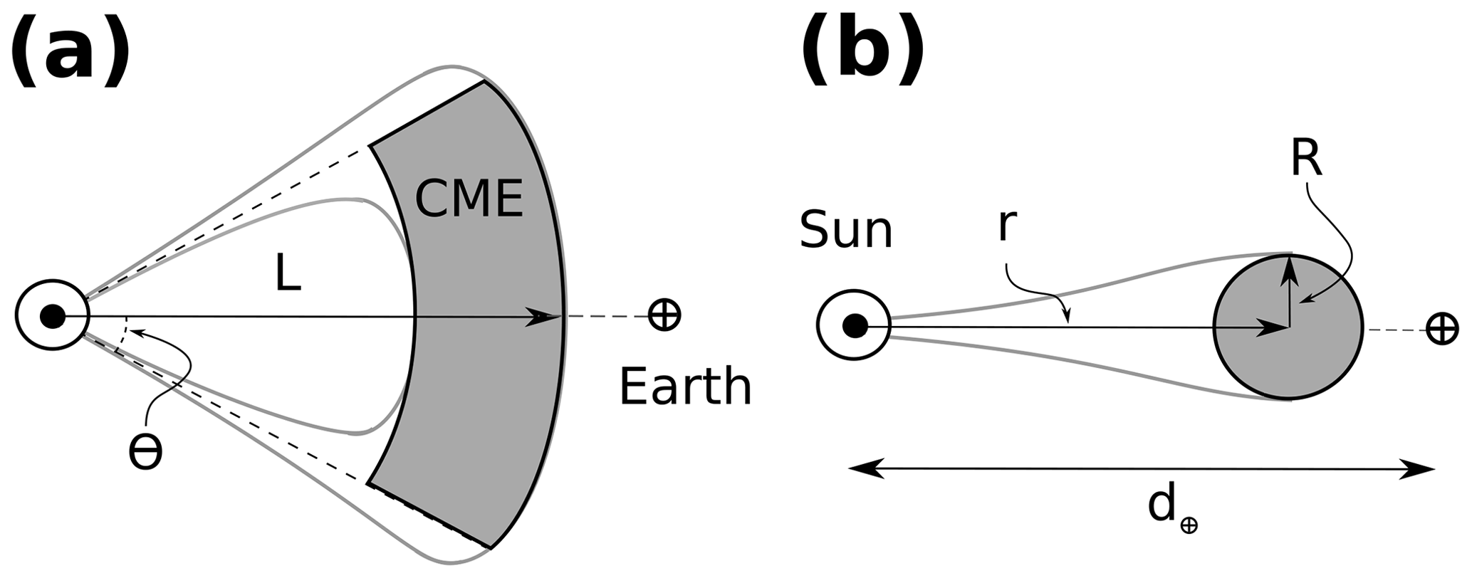
Figure 1 Sketch for the croissant-like geometry (thick solid grey line) of CMEs assumed in this work. Panels (a) and (b) show a meridian and equatorial view of the CME, respectively. We approximate the CME material through a cylinder (shaded region). In the panels we present the locations of the leading edge (L), center (r), and radius (R) of the CME and its semi-angular width (θ). We also present the position of the Sun (⊙) and Earth (⊕) as references.

More generally, we can express the CME center (r) as

$$\begin{array}{}\text{(5)}& r=L-R.\end{array}$$

Since R<L, we can combine Eqs. (4) and (5) and expand the result up to second order around L. The result is

$$\begin{array}{}\text{(6)}& R={\displaystyle \frac{\mathrm{1}+R_L^{\prime }-\sqrt{(\mathrm{1}+R_L^{\prime }{)}^{\mathrm{2}}-\mathrm{2}{R}_L{R}_L^{\prime \prime }}}{R_L^{\prime \prime }}},\end{array}$$

where we have used R_L=R(L). Additionally, $R_L^{\prime }=\mathit{ϵ}{R}_L/L$ and $R_L^{\prime \prime }=\mathit{ϵ}(\mathit{ϵ}-\mathrm{1})R_L/L^{\mathrm{2}}$ are the first and second derivatives of R_L, respectively. By combining Eqs. (6) and (5) we can express the CME center position as a function of L, i.e., Eq. (1).

Taking the time derivative of Eq. (6), we obtain the expansion speed of CMEs ($\dot{R}$):

$$\begin{array}{}\text{(7)}& \begin{array}{rl}{\displaystyle \frac{\dot{R}}{\dot{L}}}& =\mathrm{1}-{\displaystyle \frac{R_L^{\prime \prime \prime }}{(R_L^{\prime \prime }{)}^{\mathrm{2}}}}\left(R_L^{\prime }+\mathrm{1}\right)\\ & +{\displaystyle \frac{(\mathrm{1}+R_L^{\prime }{)}^{\mathrm{2}}{R}_L^{\prime \prime \prime }-(R_L^{\prime \prime }{)}^{\mathrm{2}}-R_L{R}_L^{\prime \prime }{R}_L^{\prime \prime \prime }}{(R_L^{\prime \prime }{)}^{\mathrm{2}}\sqrt{(\mathrm{1}+R_L^{\prime }{)}^{\mathrm{2}}-\mathrm{2}{R}_L{R}_L^{\prime \prime }}}},\end{array}\end{array}$$

with $R_L^{\prime \prime \prime }=\mathit{ϵ}(\mathit{ϵ}-\mathrm{1})(\mathit{ϵ}-\mathrm{2})R_L/L^{\mathrm{3}}$ being the third derivative of R_L. It follows that the speed of the CME center ($\dot{r}$) is given by the time derivative of Eq. (5):

$$\begin{array}{}\text{(8)}& \dot{r}=\dot{L}-\dot{R}.\end{array}$$

Again, by combining Eqs. (2), (7), and (8) we can express the CME center speed through the speed of the CME leading edge. Additionally, we can estimate the travel time (TT_r) of the CME “center” (r), or CME axis, by

$$\begin{array}{}\text{(9)}& \begin{array}{rl}{\displaystyle \frac{{\mathrm{TT}}_r}{{\mathit{\tau }}_f}}& =a^{\mathrm{2}}c+{\displaystyle \frac{d_{\oplus }+R_{\oplus }-L_{\mathrm{0}}}{u_{\mathrm{1}}{\mathit{\tau }}_f}}\\ & -\sqrt{\mathrm{2}ac\left(a-\mathrm{1}\right)\left[{\displaystyle \frac{d_{\oplus }+R_{\oplus }-L_{\mathrm{0}}}{u_{\mathrm{1}}{\mathit{\tau }}_f}}\right]+a^{\mathrm{2}}c\left(a^{\mathrm{2}}c-\mathrm{1}\right)},\end{array}\end{array}$$

where $R_{\oplus }=R\left(d_{\oplus }\right)$. Equation (9) was obtained by solving Eq. (1) for the condition $L=d_{\oplus }+R$.

Once the CME center position and radius are known, the piston-shock model allows us to calculate the CME mass, which depends on the initial conditions and shape of the CME (see discussion in Corona-Romero et al., 2017). For simplicity, if we assume the CME mass uniformly distributed within its volume, we can express the CME density (ρ) as

$$\begin{array}{}\text{(10)}& \mathit{\rho }=ac{m}_{\mathrm{p}}{n}_{\mathrm{1}}{u}_{\mathrm{1}}{\mathit{\tau }}_f\left[{\displaystyle \frac{{\mathit{\theta }}_{\mathrm{0}}{d}_{\oplus }^{\mathrm{2}}{R}_{\mathrm{0}}}{\mathrm{2}\mathit{\theta }{r}_{\mathrm{0}}r{R}^{\mathrm{2}}}}\right],\end{array}$$

where n₁ is the in situ solar wind proton density, m_p is the proton mass, and θ is the semi-angular width of CMEs; additionally the index “0” denotes initial values (at t=0). It is important to note that in Eq. (10) we also assume the CME mass is conserved, a condition that might be violated when significant magnetic reconnection occurs between the CME and its surrounding solar wind (e.g., Dasso et al., 2007).

2.2 Calculating in situ transit profiles of CMEs

Next, we present our procedure for calculating the synthetic transit profiles of CMEs. For simplicity, we use an astronomical unit (AU) to compute our synthetic transits; however, our equations could be easily adapted for other heliocentric distances. We also assume that the spacecraft (i.e., Earth) and the trajectory of the CME center are almost aligned; that is, the spacecraft crosses near the CME center. This simplification allows us to neglect projection effects as a first approximation but limits our formalism to CMEs whose source region is located near the center of the solar disk. We leave the solution of a more general scenario for future studies.

We will use Event 1 from Table 1 to illustrate the steps of our formalism. Figure 2 shows the in situ measurements (solid and dotted black lines) during the transit of Event 1 past Earth. From top to bottom the panels show the magnitude of solar wind radial speed ($\left|V^x\right|$), density (N_p) and temperature (T_p) of protons, and magnetic field magnitude (B). In the left-most portion of all the panels we observe ambient solar wind up to the shock arrival (8 June 2000, 09:10 UT), which is a spontaneous jump in all in situ measurements. After the shock comes the solar wind is perturbed by the shock (sheath) and, behind it, the CME. We note that during the CME transit the plasma-β (grey solid line in N_p panel) significantly decreases, and the value of T_p is lower than the expected temperature of protons (grey solid line in the T_p panel). Following the CME, there is again ambient solar wind.

Table 1 Input data for our analysis. From left to right: event number, CME detection date and time, associated active region position on the solar disk (latitude and longitude), rise time of associated solar flare, initial position and speed of the CME leading edge, in situ values of the proton density and speed of solar wind ahead (index “1”) and behind (index “2”) CMEs, and travel and transit times.

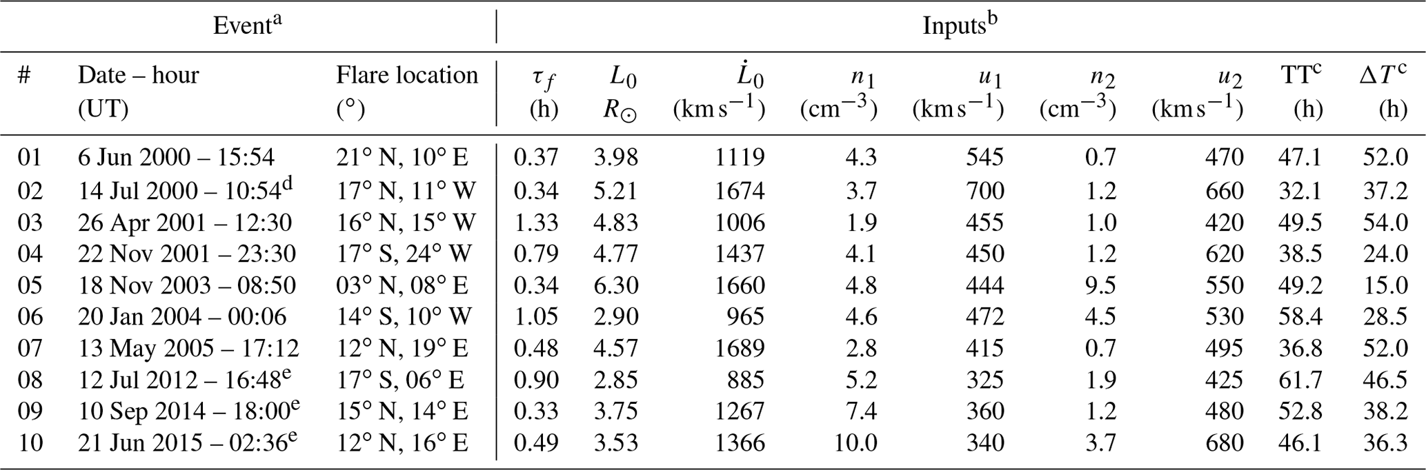
^a Detection time and inputs are reported in the LASCO CME Catalog (http://cdaw.gsfc.nasa.gov/CME_list/, last access: 14 May 2019). ^b Input data were acquired from the LASCO CME Catalog, GOES X-ray flux (https://sxi.ngdc.noaa.gov/, last access: 14 May 2019), and in situ data by OMNIWeb (http://omniweb.gsfc.nasa.gov/, last access: 14 May 2019). ^c The values of TT and ΔT were computed by identifying the transit of the events on in situ registers. In order to do so, we use the well-known in situ CME signatures (Zurbuchen and Richardson, 2006), complemented by data in the Richardson and Cane (2010) CME table that lists the LASCO detection for each event and its in situ arrival and departure dates and times, between other data (http://www.srl.caltech.edu/ACE/ASC/DATA/level3/icmetable2.htm, last access: 14 May 2019). ^d Case 2 is the Bastille Day event. ^e varSITI Campaign events (http://www.varsiti.org/, last access: 14 May 2019).

Our first step is to measure the travel time (TT) spent by the CME leading edge in traveling from near the Sun (reported detection time) to Earth's orbit (in situ detection). We mark the CME arrival time by a vertical dotted red line on the left-hand side of the panels in Fig. 2, and the corresponding TT would be the time lapse in between the arrival and detection times. With the value of TT known, we proceed to find the value of c (through Eq. 1) that makes $L\left(\mathrm{TT}\right)=d_{\oplus }$. We used the initial position, at the first appearance in C2, and the linear speed reported by the CME LASCO Catalog (Yashiro et al., 2004; Gopalswamy et al., 2009) as inputs for the values of L₀ and ${\dot{L}}_{\mathrm{0}}$, respectively. Additionally, the horizontal solid green lines in the panels of Fig. 2 mark out the solar wind values used in our calculations, values taken around 18–10 h before the CME's arrival. Table 1 lists the input values used in the analysis of Event 1.

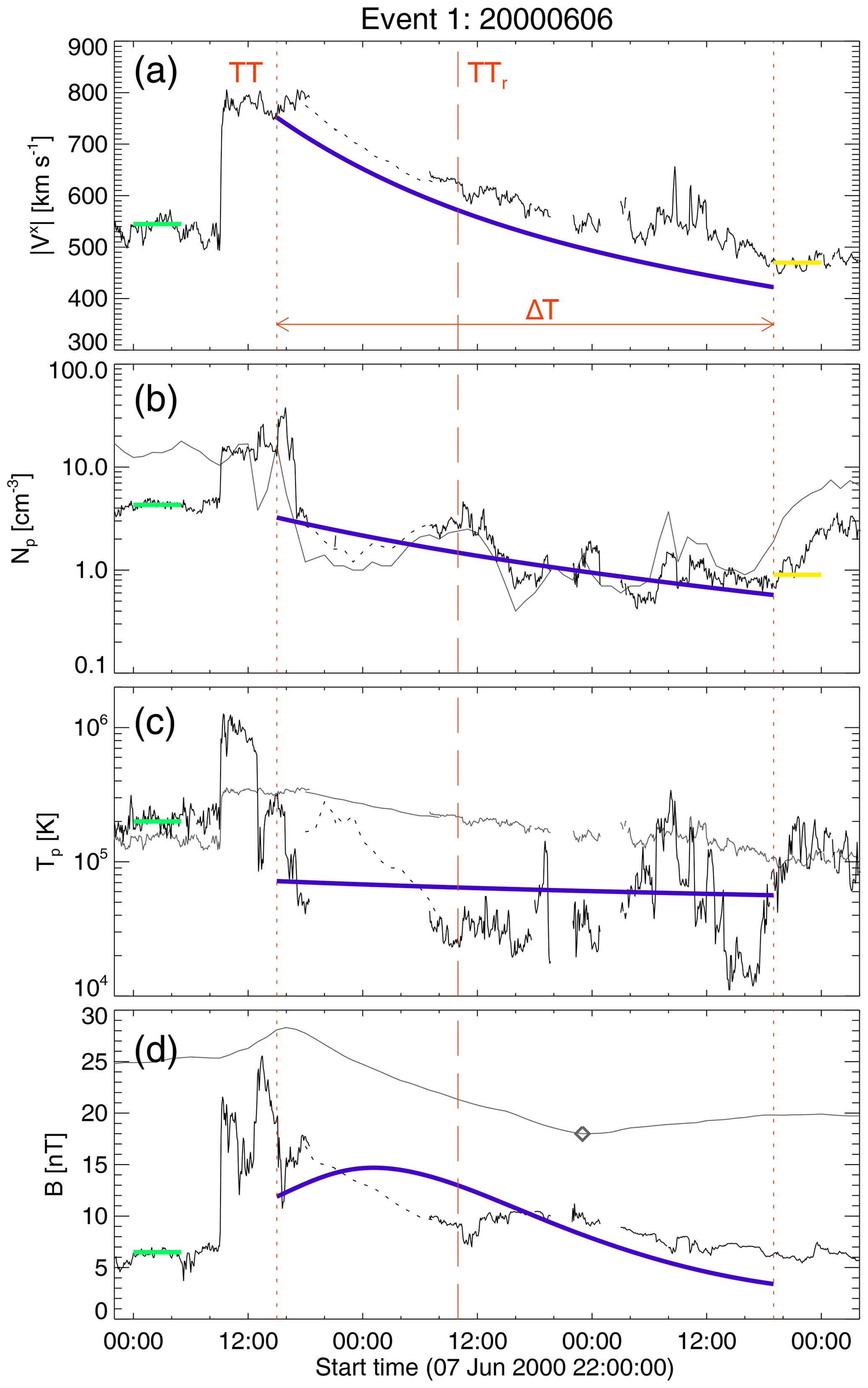
Figure 2 Calculated synthetic transit of Event 1. From top to bottom, panels (a), (b), (c), and (d) present the radial component of the solar wind speed ($\left|V^x\right|$), the density (N_p) and temperature (T_p) of protons and the magnetic field intensity (B), respectively. Solid blue lines show our model results and the solid (dotted) black lines are 5 min (1 h) resolution in situ measurements as extracted from NASA/GSFC's OMNI data set through the OMNIWeb service. Short-dashed and long-dashed vertical red lines mark the CME boundaries and center, respectively. Solid grey lines in N_p and T_p panels are the plasma-β (10 folded) and the expected proton temperature (T_exp) (Lopez, 1987; Richardson and Cane, 1993, 1995), respectively. Solid grey line in (d) is the accumulative magnetic flux, as defined by Dasso et al. (2006), whose extremum (open diamond) gives an estimation for the magnetic center inside the CME. The green solid lines, on the left-hand side of all panels, mark the in situ solar wind values used as inputs for our calculations; and solid yellow lines, in the $\left|V^x\right|$ and N_p panels, mark speed and proton density values of the solar wind behind the CME (see Table 1).

The second step is to measure the time required for the CME to cross Earth's orbit, i.e., the transit time (ΔT). In Fig. 2a we enclosed ΔT with dotted red lines; the left line marks the CME arrival, whereas the right line marks the trailing edge of the CME. Hence, at the time $t=\mathrm{TT}+\mathrm{\Delta }T$ the separation between the CME leading edge and Earth's orbit would be 2 R. Thus, after combining and manipulating Eqs. (1) and (4), we obtain

$$\begin{array}{}\text{(11)}& k=\left({\displaystyle \frac{L(\mathrm{TT}+\mathrm{\Delta }T)-d_{\oplus }}{\mathrm{0.24}{d}_{\oplus }}}\right){\left({\displaystyle \frac{\mathrm{2}{d}_{\oplus }}{L(\mathrm{TT}+\mathrm{\Delta }T)+d_{\oplus }}}\right)}^{\mathit{ϵ}}.\end{array}$$

Since we already know the values of TT and ΔT, Eq. (11) allows us to compute the value of the free parameter k, for a given value of ϵ.

Once the values of the free parameters c and k are known, in our third step we compute the trajectory (Eqs. 1 and 2), radius (Eq. 6), and expansion rate (Eq. 7 of the CME during the period $\mathrm{TT}<t<\mathrm{\Delta }T+\mathrm{TT}$. Following this, we can express the speed (V^x) on the Sun–Earth line that would be “observed” in situ:

$$\begin{array}{}\text{(12)}& \begin{array}{rl}{V}^x& =\dot{r}+\left({\displaystyle \frac{d_{\oplus }-r}{R}}\right)\dot{R}\\ & =\dot{L}+\left({\displaystyle \frac{d_{\oplus }-L}{R}}\right)\dot{R}.\end{array}\end{array}$$

In Eq. (12) we assumed that the velocity of CME material linearly grows with the radial distance from the CME axis (see Démoulin and Dasso, 2009). We overplot our calculated in situ speed (solid blue line) in Fig. 2a. We note that our calculated speed closely follows its measured counterpart; however, the synthetic profile is below the in situ data. In the general case, this issue might be fixed by using values of ${\dot{L}}_{\mathrm{0}}$ calculated by multiple spacecraft (when available) instead of using coronagraph images from one spacecraft. This is because speeds are underestimated by simple coronagraph images due to projection effects. For our example case, this was not possible since STEREOs were launched in 2006.

The fourth step consists of calculating the density and temperature profiles. Since the CME mass is homogeneously distributed, the density of protons (N_p) seen at in situ locations is expressed by

$$\begin{array}{}\text{(13)}& N_{\mathrm{p}}=\left[{\displaystyle \frac{ac{n}_{\mathrm{1}}{u}_{\mathrm{1}}{\mathit{\tau }}_f}{\mathrm{1}+\mathrm{4}{q}_{\mathit{\alpha }}}}\right]\left[{\displaystyle \frac{{\mathit{\theta }}_{\mathrm{0}}{d}_{\oplus }^{\mathrm{2}}{R}_{\mathrm{0}}}{\mathrm{2}\mathit{\theta }{r}_{\mathrm{0}}r{R}^{\mathrm{2}}}}\right].\end{array}$$

In the last expression, we depart from Eq. (10) by assuming an average ratio q_α between alpha particles and protons inside the CME. Additionally, for simplicity, we assumed a constant value for θ and a content of 12 % fraction of alpha particles in the CME material (Borrini et al., 1982; Zurbuchen and Richardson, 2006); however, the content of alpha particles can be easily modified to another value. Since we assume the CME material to be a polytropic gas, we can express the temperature of protons (T_p) by combining Eq. (10) and the well-known expression for the temperature of a polytropic gas with polytropic index γ, and, after some manipulation,

$$\begin{array}{}\text{(14)}& {\displaystyle \frac{T_{\mathrm{p}}}{T^{*}}}=\mathrm{35}\mathrm{401}\mathrm{K}{\left[{\displaystyle \frac{N_{\mathrm{p}}}{N_{\mathrm{p}\mathrm{1}}}}\right]}^{(\mathit{\gamma }-\mathrm{1})},\end{array}$$

where N_p1 is the CME proton density at $r=d_{\oplus }$ and T^* a free parameter that indicates whether the CME is hotter ($T^{*}>\mathrm{1}$) or colder ($T^{*}<\mathrm{1}$) than the approximated average temperature (35 401 K) in CMEs (see Liu et al., 2005). We selected the value of T^* that allowed the median of Eq. (14) to match the median of in situ temperature during ΔT.

Regarding the polytropic behavior of the CME material, a theoretical approach by Chen and Garren (1993) showed that an adiabatic expansion ($\mathit{\gamma }=\mathrm{5}/\mathrm{3}$) of flux ropes may derive into temperatures lower than expected. This work was followed by others that used $\mathrm{1}<\mathit{\gamma }<\mathrm{5}/\mathrm{3}$ for studying magnetic clouds (e.g., Gibson and Low, 1998; Chen, 1996; Krall et al., 2000). Afterwards, Liu et al. (2005) studied statistical properties of CMEs; one of those properties was the thermodynamics of CMEs, finding that $\mathit{\gamma }=\mathrm{1.14}\pm \mathrm{0.03}$, the value that we use in our calculations. Once more, we present our equations in such a way that facilitates the usage of a value of γ different to the one we use.

It is widely known that the Lundquist (1951) solution of a stationary flux rope's magnetic field is a useful tool to approximate magnetic fields of magnetic clouds (e.g., Burlaga, 1988; Chen, 1989; Farrugia et al., 1995; Dasso et al., 2003, 2007; Riley et al., 2004b; Liu et al., 2008, and many others). Such a solution has been extended for a number of scenarios (Vandas et al., 2006, discussed some of them). One of those extensions is the work by Shimazu and Vandas (2002), who found that polar and axial components, and thus the magnitude, of the Lundquist solution change at the same rate for a flux rope that simultaneously expands and elongates. In addition, there is empirical evidence that indicates magnetic field intensity of CME decreases with the growth of the heliocentric distance (e.g., Liu et al., 2005; Leitner et al., 2007). Furthermore, such a decrease can be approximated as a self-similar relation of r (e.g., Bothmer and Schwenn, 1998; Wang et al., 2005; Liu et al., 2005; Forsyth et al., 2006; Leitner et al., 2007, and others), a relation that was theoretically explored by Gulisano et al. (2010).

Thus, to keep our expression as simple as possible, it is reasonable to locally approximate the in situ magnetic field magnitude of CMEs (B) by

$$\begin{array}{}\text{(15)}& \begin{array}{rl}{\displaystyle \frac{B}{b}}& =\mathrm{10.9}\mathrm{nT}{\left[{\displaystyle \frac{r}{d_{\oplus }}}\right]}^{-\mathrm{1.85}}\\ & \times \sqrt{J_{\mathrm{0}}^{\mathrm{2}}\left(\mathit{\alpha }{\displaystyle \frac{|d_{\oplus }-r|}{R}}\right)+J_{\mathrm{1}}^{\mathrm{2}}\left(\mathit{\alpha }{\displaystyle \frac{|d_{\oplus }-r|}{R}}\right)},\end{array}\end{array}$$

where the square root in Eq. (15) is the magnitude of the Lundquist solution, with J₀ and J₁ the first and second Bessel functions, respectively, and α the J₀'s first zero. In addition, the other terms on the right-hand side of Eq. (15) correspond to the empirical tendency reported by Gulisano et al. (2010) that controls the decaying rate of the magnetic field magnitude as heliocentric distance (time) grows larger.

In Eq. (15) we introduced the non-dimensional free parameter b to express stronger (b>1) or weaker ($\mathrm{0}<b<\mathrm{1}$) intensities of the CME magnetic field, in comparison with the average value of 10.9 nT (see Gulisano et al., 2010). Hence, our fifth step is to calculate the value of b, whose value we select to minimize the average error in our calculated intensity of the magnetic field:

$$\begin{array}{}\text{(16)}& {\mathit{\epsilon }}_B={\displaystyle \frac{\mathrm{1}}{N}}\sum _{i=\mathrm{1}}^N|B_i^{\mathrm{calc}}-B_i^{\mathrm{in}\mathrm{situ}}|,\end{array}$$

where N is the number of available data points during the CME in situ transit, and B^calc and B^in situ correspond to the calculated and measured in situ magnetic field intensities, respectively.

Although Eq. (15) may share similarities with other physics-based expressions (e.g., Farrugia et al., 1993; Cid et al., 2002; Berdichevsky et al., 2003; Nakwacki et al., 2008; Möstl et al., 2009; Vandas et al., 2009; Mingalev et al., 2009; Nieves-Chinchilla et al., 2016, and many others), we emphasize that such an equation is a simplified straightforward expression to estimate representative data. Nevertheless, we anticipate that Eq. (15) is consistent with a particular case of the physical model by Démoulin et al. (2008), as we will discuss latter in Sect. 4. This point is important and in contrast with other works, because Démoulin et al. (2008) simultaneously include radial and axial expansions of the flux rope as well as the acceleration on CME bulk speed.

Finally, our last step is to calculate the travel time associated with the CME center (TT_r), which is done by Eq. (9) and for which the parameters are already known. The calculated moment at which the CME center transits Earth's orbit is shown with a vertical dashed red line in all panels of Fig. 2. We compare our calculated value for TT_r with the extremum (open diamond) of the accumulative magnetic flux per unit length (solid grey line) in panel (d) (Dasso et al., 2006). In order to compute it, we integrate the (poloidal) magnetic field component that is simultaneously perpendicular to the propagation direction and axial component, along the spacecraft transit inside the CME. For this purpose, we use the maximum variance technique to infer the reference frame of the CME magnetic field and use the magnetic coordinate of the largest variance to calculate the accumulated magnetic flux as a function of time. It is important to note that this extremum gives an estimation for the time of closest approach to the magnetic center inside the CME.

3 Testing our formalism

To explore the ability of our formalism to approximate in situ transit profiles of CMEs, we analyzed 10 Earth-directed halo CMEs listed in Table 1. The events were selected from the LASCO Catalog (Gopalswamy et al., 2009) and occurred during the 2000–2015 period. The objective of our selection criteria was to isolate events that fulfilled most of our formalism's assumptions and consisted of five points: (1) fast CMEs according to coronagraph images (${\dot{L}}_{\mathrm{cme}\mathrm{0}}>\mathrm{800}$ km s⁻¹), to ensure the effectiveness of a piston-shock approximation to model the CME trajectory; (2) CMEs associated with solar flares for which the active region was located near the solar disk center, to reduce in situ geometrical effects on propagation and expansion speeds of CMEs; (3) CMEs that were almost isolated (not complex) events preceded by an observed shock wave in situ and in situ signatures that were clear enough to be detected; (4) the ambient solar wind (at 1 AU) was stable enough about 12 h before the ICME-shock arrival in order to assume an almost quiet solar wind. Table 1 lists the events studied and the inputs used in our calculations.

We calculated the synthetic in situ profiles and CME center travel time for Events 2–10 by following the procedure we described in Sect. 2.2 for Event 1. We present our results in Figs. 4 and 5 following a similar format to that used in Fig. 2. The figures show the in situ measurements (solid black lines) of radial speed, density and temperature of protons, and magnetic field magnitude, as well as the calculated travel time for the CME center (vertical red-dashed lines). Solid grey lines in the N_p, T_p, and B panels are the plasma Beta (multiplied by 10), the expected temperature of protons (Lopez, 1987; Richardson and Cane, 1993, 1995), and the accumulative magnetic flux (Dasso et al., 2006) in arbitrary units, respectively. On the left-hand side of all speed and proton density panels, we highlight the in situ solar wind conditions used as inputs (solid green lines), and the CME boundaries are marked by vertical dotted red lines.

Table 2 and Fig. 3 provide general insight about our results, since they present the absolute and proportional errors associated with our calculations, respectively. It is important to highlight that in both the table and the figure we used the absolute difference between our calculations and in situ measurements as error, in a similar way we did for ε_B (Eq. 16). According to Fig. 3, our results with lower errors are the calculated TT_r (purple bars), and the synthetic transits of speed (cyan bars) and magnetic intensity (yellow bars), with average proportional errors of 8.7 %, 9.6 %, and 27 %, respectively.

Table 2 Results from our analysis. From the left to the right: event number, CME detection date and time, values of free parameters, and associated errors with our calculated results.

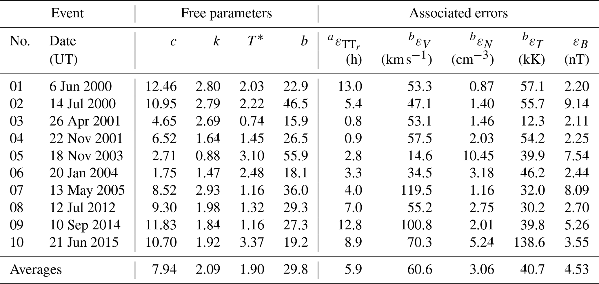
^a Absolute error when compared with the extreme value of magnetic flux detection time. ^b Associated errors with speed (ε_V), density (ε_N), and temperature (ε_T) profiles are calculated with expressions similar to Eq. (16) but using the values of speed, densities, and temperatures instead of magnetic field.

In contrast, the proportional errors for temperature (green bars) and density (orange bars) of protons were significantly larger than the first ones, with values of 83 % and 143 % as averages, respectively. Although the errors for temperature and density are remarkably large, we found that such large errors are driven by inherent properties of the in situ data. For example, when we calculate the error between measured and calculated median values of proton density (${\mathit{\epsilon }}_{<N>}$) instead of the average error for all the data points (ε_N), we found that ${\mathit{\epsilon }}_{<N>}$ drops to ∼101 %. In addition, when we neglect those events that broke our homogenous solar wind assumption, i.e., those events affected by interacting streams of solar wind, such an error falls to 46 %. We discuss our results in the next sections.

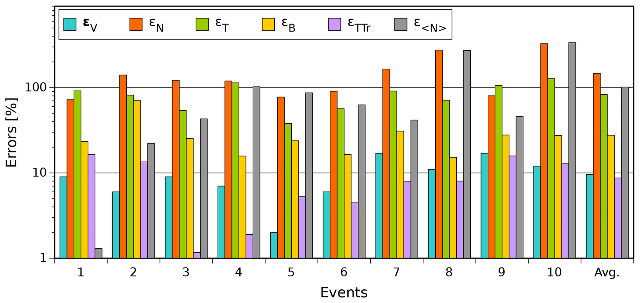
Figure 3 Proportional error histograms associated with our calculated synthetic profiles for speed (cyan), proton density (orange), temperature (green), and magnetic field (yellow). The last set of bars corresponds to the averaged values. Additionally, grey bars are the errors when comparing the median values of proton density (${\mathit{\epsilon }}_{<N>}$); and purple ones correspond to the error when comparing the TT_r with the transit of the accumulative magnetic field flux's extremum.

3.1 Synthetic profiles of speed

According to Fig. 3, the calculated speed profiles accurately resemble their observed in situ registered counterparts with proportional errors below 17 %. Our speed results had the best performance between synthetic profiles with an average error of 61 km s⁻¹ (∼10 %), which is not significant when compared with in situ transit speeds of CMEs (400–1000 km s⁻¹). In Figs. 2, 4, and 5 we note that synthetic speed profiles (solid blue lines) closely follow the in situ measurements (grey lines) for all cases. It is important to note that calculated profiles are systematically lower than their in situ observed counterparts. However, in the best (worst) of the cases, such a systematic underestimation derived into an average difference of 15 km s⁻¹ (119 km s⁻¹), i.e., a difference of 2.4 % (17.0 %); see Table 2.

It is important to note that all of our synthetic speed profiles reproduce the monotonic speed-decreasing tendency called aging (Osherovich et al., 1993), commonly associated with the CME expansion. The aging effect refers to the change in the CME characteristics seen in in situ registers during the spacecraft transit across the CME structure; such a change is mainly due to the CME expansion. The aging effect is also present in the in situ data; however, it varies from one event to another, a condition that is easily observed in synthetic profiles. For example, on the one hand, we have Event 7 for which the speed profile decreases with a pronounced curve-like shape (see Fig. 5). On the other hand, the speed profile of Event 5 decreases almost like a line of constant slope. It is widely accepted that the difference between the “initial” and “final” in situ speeds of a CME is directly related to the magnitude of its expansion speed. However, the source of the “curve-like” or “constant-slope” shapes is not commonly discussed. Furthermore, as is well known, to have curvature in the speed vs. time profile requires a net acceleration; in our case, such an acceleration is related to the change (deceleration) in expansion speed ($\mathrm{\Delta }\dot{R}$) during ΔT.

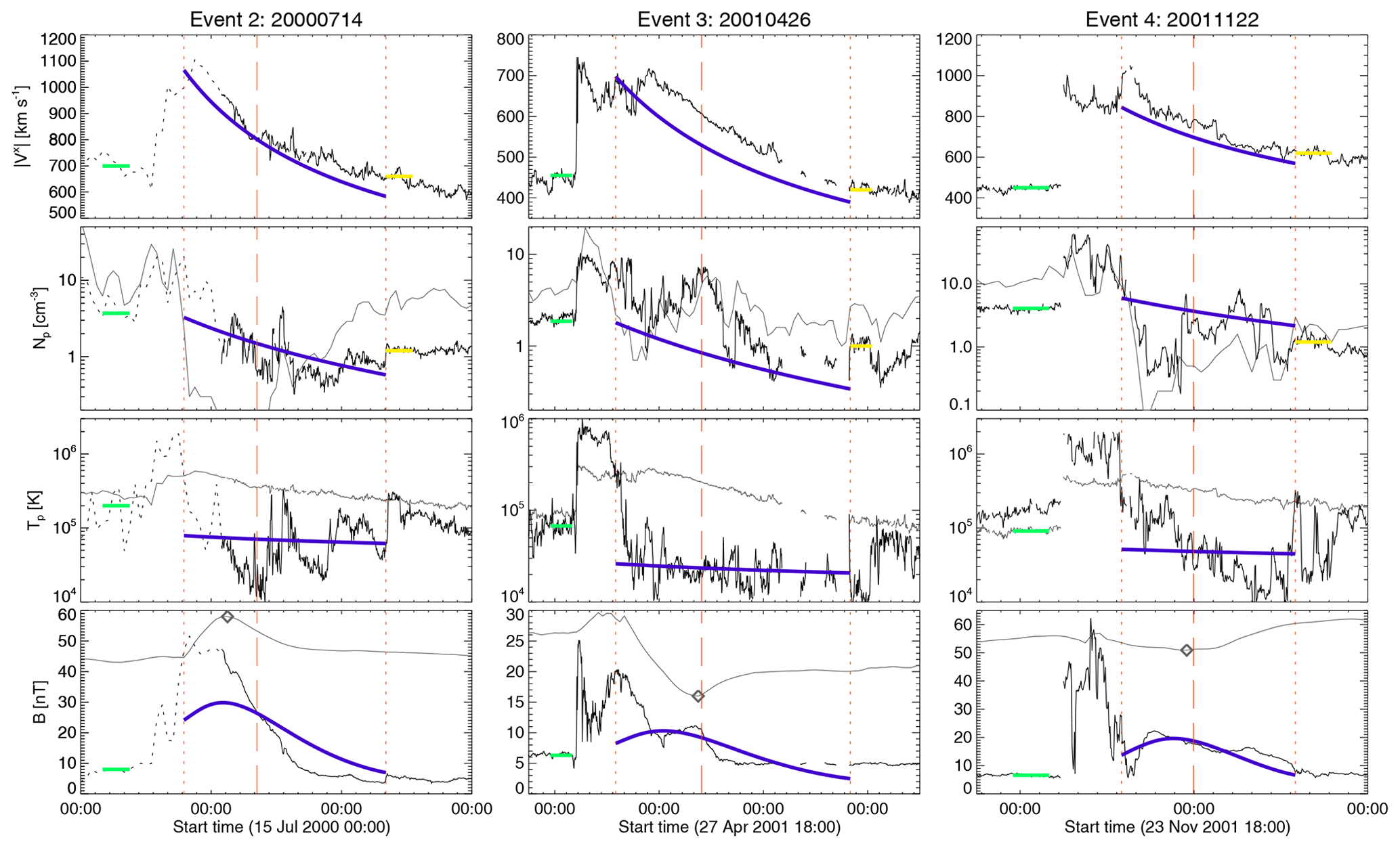
Figure 4 Calculated synthetic transit of Events 2, 3, and 4; each column shows a different event. From top to bottom, the panels present the radial component of the solar wind speed ($\left|V^x\right|$), the density (N_p) and temperature (T_p) of protons and the magnetic field intensity (B). Solid blue lines are our model results. Short-dashed and long-dashed vertical red lines mark the CME boundaries and center, respectively. The solid (dotted) black lines are 5 min (1 h) in situ measurements as extracted from NASA/GSFC's OMNI data set through the OMNIWeb service. Green solid lines mark in situ solar wind used for calculations (see Table 1). The solid grey lines in N_p and T_p panels are the plasma beta (10 folded) and the expected proton temperature (T_exp) (Lopez, 1987; Richardson and Cane, 1993, 1995), respectively. The solid grey line in the B panel is the accumulative magnetic flux, as defined by Dasso et al. (2006), whose extremum (open diamond) gives an estimation for the magnetic center inside the CME.

Figure 5 Calculated synthetic transit of Events 5 to 10. We present two rows with three columns each; and each column of four panels shows a different event. From top to bottom, the panels present the radial component of the solar wind speed ($\left|V^x\right|$), the density (N_p) and temperature (T_p) of protons and the magnetic field intensity (B). Solid blue lines summarize our model results. Short-dashed and long-dashed vertical red lines mark the CME boundaries and center, respectively. Dotted red lines mark the CME boundaries. The solid (dotted) black lines are 5 min (1 h) in situ measurements from the OMNIWeb service. Green solid lines mark in situ solar wind used for calculations (see Table 1). The solid grey lines in the N_p and T_p panels are the plasma Beta (10 folded) and the expected proton temperature (T_exp) (Lopez, 1987; Richardson and Cane, 1993, 1995), respectively. The solid grey line in B panel is the accumulative magnetic flux, as defined by Dasso et al. (2006), whose extremum (open diamond) gives an estimation for the magnetic center inside the CME.

Figure 6 shows four panels related to changes in CME speeds during ΔT. Panel (a) shows a histogram with the proportional changes for the CME center ($\mathrm{\Delta }\dot{r}/\dot{r}$, cyan bars) and expansion ($\mathrm{\Delta }\dot{R}/\dot{R}$, blue bars) speeds during ΔT for all the events, and the averages (rightmost bars). We note that, on average, the proportional changes on $\dot{r}$ (−8.2 %) are small when compared with those of $\dot{R}$ (−19.2 %), a condition that suggests $\mathrm{\Delta }\dot{R}$ as a source of the curve-like shapes for speed profiles. Note also that $\mathrm{\Delta }\dot{R}$ covers a wide range of values, where the previously described Events 5 and 7 are two extreme examples, with values for $\mathrm{\Delta }\dot{R}$ of ∼9 % and −31.5 %, respectively.

Figure 6 The changes in $\dot{R}$ and $\dot{r}$ during ΔT. (a) Histogram of the proportional variations of the CME center ($\mathrm{\Delta }\dot{r}$) and expansion ($\mathrm{\Delta }\dot{R}$) speeds with respect to $\dot{r}\left({\mathrm{TT}}_r\right)$. The right-most columns are the average values of $\mathrm{\Delta }\dot{r}$ and $\mathrm{\Delta }\dot{R}$, respectively. (b) Data dispersion of ΔT_a∕ΔT_b as a function of $\mathrm{\Delta }\dot{R}$ (black diamonds) and $\mathrm{\Delta }\dot{r}$ (open circles) also. The dotted line represents the calculated regression for the tendency with $\mathrm{\Delta }\dot{R}$ as a variable. (c) $\mathrm{\Delta }\dot{R}$ as a function of the free parameter k. The dashed line is the theoretical approximation given by Eq. (17), and the error bars are the difference between the average error of $\mathrm{\Delta }\dot{r}$ and its maximum value, according to (b). (d) $\mathrm{\Delta }\dot{r}$ as a function of the difference between the calculated arrival speed of the CME leading edge and the ambient solar wind. The dashed line is the tendency regression calculated for the data dispersion.

In the case of Event 5, the value of $\mathrm{\Delta }\dot{R}$ allows us to assume that $\dot{R}$ is almost constant during ΔT, a condition that provokes the “constant slope” shape in the speed profile of Event 5 (see Fig. 5) due to the absence of accelerations during ΔT ($\mathrm{\Delta }\dot{R}\sim \mathrm{0}$ and $\mathrm{\Delta }\dot{r}\sim \mathrm{0}$). We can verify this in Event 6 ($\mathrm{\Delta }\dot{r}\sim \mathrm{11}$ %), which also shows the constant-slope speed profile (see Fig. 5). In contrast to Event 5, Event 7 has a value of $\mathrm{\Delta }\dot{R}$ (−31.5 %), far above the average, with deceleration that provokes the curve-like speed profile. We can corroborate this in other cases with high decelerations like Events 2 and 3, with values of $\mathrm{\Delta }\dot{R}\sim -\mathrm{22}$ % that also present the curve-like shape (see Fig. 4).

To verify the influence of $\mathrm{\Delta }\dot{R}$ on the apparent curvature due to the aging, we examined how soon a CME center passes by the orbit of Earth. We do so by comparing the calculated transit times of the half-ahead region (ΔT_a) of CMEs with their behind counterparts (ΔT_b). Figure 6b shows the ratio ΔT_a∕ΔT_b as a function of $\mathrm{\Delta }\dot{R}$ (solid diamonds) and $\mathrm{\Delta }\dot{r}$ (open circles) for completeness. In the panel we note a relationship between $\mathrm{\Delta }\dot{R}$ and the transit times ratio (dotted line). In contrast, there is no clear relation for the case of $\mathrm{\Delta }\dot{r}$.

This tendency indicates that ΔT_a≪ΔT_b for large decelerations ($\mathrm{\Delta }\dot{R}\ll \mathrm{0}$), and the transit times ratio gradually grows larger as $\mathrm{\Delta }\dot{R}$ approaches zero. The tendency suggests that, when the deceleration is negligible ($\mathrm{\Delta }\dot{R}\sim \mathrm{0}$), ΔT_a∼ΔT_b; i.e., the CME center crosses Earth's orbit almost at the midpoint of ΔT, these being the conditions for a constant slope speed profile. In contrast, when $\mathrm{\Delta }\dot{R}\ll \mathrm{0}$, the CME center crosses early, compared with ΔT, at the orbit of Earth. This early passage of the CME center constrains all the leading material of a CME to rapidly pass through the point of measurement while forcing the delayed trailing material to a slow crossing through Earth's orbit. These conditions became the curve-like profiles observed for large decelerations.

Due to the importance of $\mathrm{\Delta }\dot{R}/\dot{R}$, we examine it through the relation $\mathrm{\Delta }\dot{R}=\ddot{R}\mathrm{\Delta }T$. To do so, we depart from Eq. (4) by assuming $\mathrm{\Delta }T\sim \mathrm{2}R/\dot{r}$ and evaluating for $r=d_{\oplus }$. After some algebra we arrive at

$$\begin{array}{}\text{(17)}& {\displaystyle \frac{\mathrm{\Delta }\dot{R}}{\dot{R}}}\sim -\mathrm{0.24}(\mathrm{1}-\mathit{ϵ})k+{\displaystyle \frac{\mathrm{\Delta }\dot{r}}{\dot{r}}}\sim -\mathrm{0.053}k-\mathrm{0.09}.\end{array}$$

Equation (17) explains the reason $\mathrm{\Delta }\dot{R}$ is systematically larger than $\mathrm{\Delta }\dot{r}/\dot{r}$ (see Fig. 6b), since it combines two independent processes: the deceleration of bulk speed and the effects of CME size. Hence, CMEs with a large radius (k≫1) or intense bulk deceleration ($\frac{\mathrm{\Delta }\dot{r}}{\dot{r}}\ll \mathrm{0}$) would have stronger radial decelerations. Nevertheless, as we commented on before, the value of ϵ may change depending on the effects of the solar wind on the expansion of CMEs.

In the particular case of the expression we are using, Gulisano et al. (2010) obtain values for ϵ of 0.89±0.15 and 0.45±0.16 for those unperturbed and most perturbed CMEs, respectively. Hence, departing from such a criterion, the expansion rate of those unperturbed CMEs (ϵ∼1) would likely depend on $\mathrm{\Delta }\dot{r}$, rather than k. In contrast, for the cases of perturbed events (ϵ<1), we expect that CME size (k) would dominate over the proportional acceleration of the CME center. We illustrate this in Fig. 6c, where we plot the values of $\mathrm{\Delta }\dot{R}$ and Eq. (17) (dashed line) as functions of k. In the panel we note that the data follow our semi-empirical tendency, particularly when considering the error bars associated with the effects of $\mathrm{\Delta }\dot{r}$. Here, we remark that the relation between CME size and expansion rate deceleration was previously reported by Démoulin et al. (2008).

In addition, although the value of $\mathrm{\Delta }\dot{r}$ is in general low, for completeness purposes we explored for the main conditions that may drive the value of bulk deceleration. We found that the relative speed between CME leading edge and solar wind ahead of the CME is a determinant factor for bulk deceleration; we can see this in Fig. 6d. In the panel we show how the proportional bulk deceleration of CMEs intensifies as the difference ${\dot{L}}_{\mathrm{1}}-u_{\mathrm{1}}$ grows larger; we also plot the regression (second-degree polynomial) for the data dispersion. In the panel we note a tendency for $\mathrm{\Delta }\dot{r}$ to decrease as the value of ${\dot{L}}_{\mathrm{1}}-u_{\mathrm{1}}$ grows larger, and it seems to vanish when the in situ speeds tend to equalize each other. Hence, faster CMEs would have stronger bulk decelerations and, in consequence, more intense expansion rate decelerations. In consequence, as long as a CME presents a self-similar-like expansion (i.e., Eq. 17), we would expect that fast CMEs with large radii would have stronger radial decelerations.

3.2 Synthetic profiles of magnetic intensity

With an average error of 4.5 nT (see Table 2), our calculations of magnetic intensity had the second best performance between synthetic profiles. In Figs. 2, 4, and 5 we note that our results (blue solid lines) qualitatively resemble the in situ data they are attempting to approximate, with most of the proportional errors in the range of 30 % and 15 % (see yellow bars in Fig. 3). However, it is important to remark that we selected the values of the free parameter b that minimized the error (ε_B) in our results, implying that our errors cannot be reduced further.

Although all our synthetic profiles showed the hill-like shape characteristic of the Lundquist solution, we found three effects that may modify the way a synthetic profile is observed: (i) the decrease in magnetic intensity due to the expansion of CMEs ($\mathrm{\Delta }\dot{R}$); (ii) the asymmetry driven by deceleration of expansion rates; and (iii) the path at which the magnetic field is “measured” (seen) inside CMEs, i.e., the impact parameter. The effects of CME expansion on the magnetic field are well known, as well as the consequences of the impact parameter for the measured data. However, the effect of $\mathrm{\Delta }\dot{R}$ is not commonly explored; to the best of our knowledge, only Démoulin et al. (2008) have discussed this topic.

Figure 7 illustrates the effects of $\mathrm{\Delta }\dot{R}$, and the impact parameter, on the observed magnetic field symmetry. Panels (a) and (c) of the figure show the synthetic profiles of the magnetic field for the events with the strongest and weakest expansion rate decelerations, respectively. If we focus on the solid bold profile (0^∘) in the bottom panel, we see a significant symmetry that makes the peak (open square) of magnetic intensity appear near (∼6 h) the midpoint (open triangle) of ΔT (∼16 h). Conversely, in the upper panel the peak of magnetic intensity occurs early during ΔT, even before the transit of the CME center (open diamond), a condition that leads to an accentuated asymmetry. Such an asymmetry is due to a process similar to the one already described in Sect. 3.1 for speeds, since most of the transit time is spent in the transit of the backside magnetic field, forcing the leading magnetic field to rapidly transit by the “spacecraft”.

In panels (a) and (c) of Fig. 7 we also show the magnetic profiles, computed for a number of angular separations between the “measurement location” and the trajectory of the CME center, that run from the complete alignment (0^∘) to a shallow transit near the CME boundary edge. It is important to comment that such an angular separation (impact parameter) relies on the CME size, the reason being that Event 7 (k=2.93) has larger angular separations than Event 5 (k=0.88). We note in both panels that the hill-like shapes gradually flatten out, and the overall intensity decreases, as the angular separation between CME and measurement location grows larger. Unexpectedly, this flattening also reduces the asymmetry in the profiles of panel (a), which starts as an accentuated asymmetric profile (0^∘) and ends as a constant-slope-like trace of short duration (20^∘), whereas the symmetry in profiles of panel (c) is barely perturbed by the angular separation, and we also observe the already commented reduction in transit times. We remark that the profiles in Fig. 8a have similar properties to those of the three groups defined by Jian et al. (2006), which used the total perpendicular pressure as a proxy to define the trajectory inside a CME-like structure.

Figure 7 Effects of trajectory and expansion rate on synthetic profiles of magnetic field intensity, and absolute error dependence on initial speeds of CMEs. (a, c) Synthetic profiles for different CME initial orientations for Events 7 (a) and 5 (c) during ΔT. The different profiles correspond to initial CME trajectories deviating from the Sun–Earth line of sight. The open squares and open diamonds point out the maximum value of $\left|B\right|$ and the closest approach to the CME center, respectively. (b) Transit of magnetic intensity peak, in terms of transit times, vs. $\mathrm{\Delta }\dot{R}$ for all events. (d) Absolute error for synthetic profiles of magnetic intensity. The calculated absolute errors as a function of ${\dot{L}}_{\mathrm{0}}$. In (b) and (d) the dashed lines are the performed regression for the data.

Hence, according to our formalism, the asymmetry of magnetic intensity profiles is closely related to $\mathrm{\Delta }\dot{R}$, as we illustrate in panel (b) of Fig. 7. The panel shows the calculated moment for the transit of magnetic intensity peaks, normalized by ΔT, as a function of $\mathrm{\Delta }\dot{R}$. We note in the panel that magnetic peaks appear early for strong decelerations; and, as the deceleration decreases, the appearance of magnetic peaks tends to delay. Furthermore, when $\mathrm{\Delta }\dot{R}\sim \mathrm{0}$ the transit of magnetic peaks is closed to ΔT∕2, as the data regression suggests (dashed line). As a consequence, due to the symmetry of magnetic profiles being mainly an effect of $\mathrm{\Delta }\dot{R}$, we expect that larger and faster CMEs would tend to have asymmetric-like magnetic intensity profiles, unlike those slow and small ones, again in agreement with the results of Démoulin et al. (2008).

In addition, we found that synthetic profiles systematically underestimated the early in situ values of the magnetic intensity of CMEs. This is particularly clear for Events 2, 7, and 9, for which the in situ data are larger than the synthetic transits. It is important to highlight that those events also had the three largest proportional errors for magnetic fields (see Fig. 3). We believe that such an underestimation derives from a compression by the solar wind that pushes back the frontal regions of CMEs in order to decelerate them, processes that simultaneously drive a geometrical deformation and an increment on magnetic intensity. In Fig. 7d we note that the absolute error for magnetic intensity (open diamonds) tends to grow larger as the initial speed of CMEs (${\dot{L}}_{\mathrm{0}}$) increases. Such a tendency (dashed line) suggests on the one hand that our formalism's ability to approximate magnetic intensity profiles relies on the initial conditions of CMEs, where faster CMEs would have larger associated uncertainties. On the other hand, due to the dependence on the initial speed of CMEs, it would be likely that the hypothetical compression on a magnetic field would occur during the early stages of CME evolution, rather than their interplanetary propagation.

Although the behavior noted above cannot be addressed by our formalism, there are attempts to theoretically solve these kinds of magnetic profiles. For example, Romashets and Vandas (2005) addressed those profiles via asymmetric magnetic fields expressed as an expansion of Bessel's functions. Another example was performed by Vandas et al. (2005), who explored the effects on magnetic profiles when an oblate shape is assumed for the flux rope.

3.3 CME center, transit times, and travel times

Understanding the geometry and trajectory of CMEs may help us identify, in in situ measurements, the transit of CMEs, their boundaries, and the closest approaches to the CME centers as well. Although it might be intuitive to relate peaks of magnetic intensity, or related quantities, to the magnetic core of CMEs (e.g., Jian et al., 2006), those peaks, however, do not necessarily approximate the moment of closest approach to the CME center. Panels (a) and (c) of Fig. 7 compare the peaks of magnetic intensity with the calculated closest approaches to the CME center (open diamonds) for a number of impact parameters for Events 7 (asymmetric profiles) and 5 (symmetric profiles), respectively. In the case of Event 7 (panel a) we note the substantial differences between the magnetic peaks and the calculated transits for the CME center (TT_r). Conversely, we note in panel (c) that peaks of magnetic intensity are systematically close (∼1 h) to TT_r (symmetric profiles), suggesting that peaks of magnetic intensity are good proxies for CME center transits in symmetric profiles only.

It could also be reasonable to assume the midpoint of the transit time (ΔT∕2) as an approximation for TT_r, values that we also plotted in panels (a) and (c) of Fig. 7 as open triangles. We see in panel (c) that TT_r is near (<1 h) to ΔT∕2, whereas in panel (a) we note that the CME center and midpoint transit times significantly differ from each other. Thus, as was the case for magnetic peaks, ΔT∕2 would approximate TT_r solely for those symmetric profiles of magnetic intensity, i.e., for small and slow CMEs. Nevertheless, we highlight that TT_r systematically falls in between the magnetic peaks and transit time midpoints, regardless of $\mathrm{\Delta }\dot{R}$ value or the impact parameter. Hence, in principle, it might be possible to approximate TT_r as the average of ΔT∕2 and the occurrence of the peak of magnetic intensity for both symmetric and asymmetric profiles.

Another method to estimate the closest approach to the CME center is the accumulated magnetic flux (AMF). As commented earlier, the AMF method uses the magnetic coordinate of largest variance to calculate the accumulated magnetic flux inside the CME structure. Once the accumulated flux is known as a function of time, this method associates the local extreme value of the AMF with the CME center's closest approach (see Dasso et al., 2006, and references therein, for further details). In Figs. 2, 4, and 5 we plot the calculated AMF as thin grey lines in magnetic intensity panels for all events. Additionally, we mark out the AMF's extreme values by open grey diamonds, values that we compared with our calculated TT_r.

Our method showed a quantitative capability to approximate CME center transits estimated by the AMF method with an average error of ∼9 % (see Fig. 3). Additionally, Table 2 shows the absolute errors (${\mathit{\epsilon }}_{{\mathrm{TT}}_r}$) associated with our results; we note that, on average, our results differ by a few hours (∼6 h) from those calculated by AMF. We highlight that such an error is small when compared with the averages of TT (∼47 h) and ΔT (∼38 h). The consistency between the data and our results can be seen in Figs. 2, 4, and 5, in which our calculated TT_r (vertical dashed red lines) are systematically close to the extremes of magnetic flux (open diamonds).

It is important to comment that the AMF method assumes a trajectory near a single magnetic structure inside CMEs. Then, large-impact parameters or imprecise CME boundaries might mislead the method's results, as well as CMEs of non-single magnetic structure. Perhaps one of them is the reason for the errors above the average (${\mathit{\epsilon }}_{{\mathrm{TT}}_r}\gg \mathrm{9}$ %) of Events 1, 2, 9, and 10. By inspecting these events we notice that their temperature profiles surpassed the expected temperature (solid grey line), a condition that could have a number of explanations. For example, it is reasonable to think of multiple magnetic structures forming the CMEs and to assume that the CME material might have been somehow externally compressed. It might also be possible that the CME boundaries are ambiguously determined, implying that we are not correctly analyzing the CMEs.

In regard to transit and travel times and the impact parameter, we note in panels (a) and (c) of Fig. 7 that ΔT is highly dependent on the trajectory at which it is “measured” (calculated). In both panels we see that ΔT is maximum when the measuring location passes by the CME center (0^∘ lines), since the whole and expanding CME is transited. After this maximum, ΔT gradually decreases as the CME trajectory moves away from the measurement location (larger angles), which reduces the CME structure “seen” at the measured location, implying that the CME radius “seen” in situ, i.e., the value of k, would be a lower limit. In contrast, we see that TT grows larger as the impact parameter gets larger. It most probably derives from the fact that the CME structure delays in being “seen” and the measured point moves away from the CME trajectory. Surprisingly, the growth of TT and the shortening of ΔT somehow equilibrate with each other to make the closest approach of the CME center (open diamonds) almost equal for all impact parameters.

3.4 Density and temperature errors

The synthetic profiles of temperature and density were the ones with the largest errors, with averages of 83 % for the first and 147 % for the latter (see Fig. 3). In particular, our density profiles systematically had errors above 70 % that reach values as large as 327 %. Such large errors represent an important limitation for our formalism. Consequently, before we discuss our results regarding temperature and density, we attempt to understand these errors. In order to do so, we depart from the fact that in situ values of density and temperature showed significant (large and fast) variations during ΔT. This behavior can be seen in Fig. 8a, where we present a histogram of the standard deviations (σ) in terms of the median values of N_p (orange) and T_p (green), during ΔT. In the panel we note that, when neglecting Events 5 and 6, the values of σ are systematically larger than their associated median values (σ>1). In the case of Events 5 and 6, we noted that their standard deviations fell near the average value; nevertheless, they also had median values far above the average. These conditions resulted in the short bars shown in the histogram in Fig. 8a.

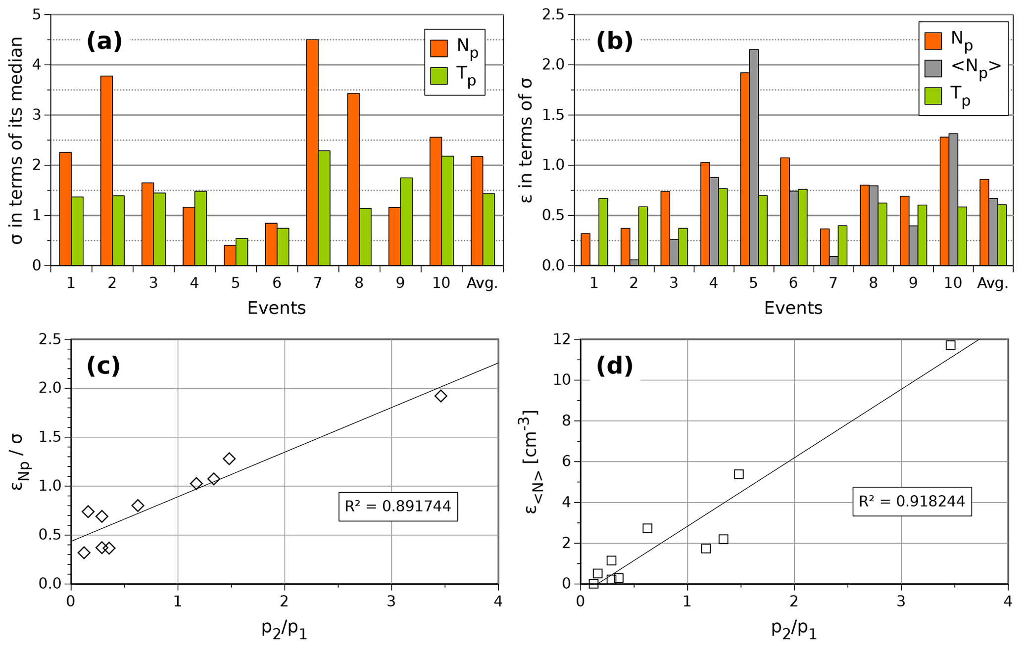
Figure 8 Histograms of the standard deviations and errors associated with the density (orange) and temperature (green) of protons, and dispersion of density errors as functions of the solar wind ram pressure quotient. (a) Standard deviation (σ) in terms of the associated median value ($<N_{\mathrm{p}}>$), both calculated for in situ data during ΔT. (b) Average errors (ϵ) associated with our synthetic profiles in terms of their corresponding standard deviations. The rightmost bars in (a) and (b) show the average values of ϵ and σ, respectively. (c) Density errors (open diamonds) in terms of their corresponding standard deviations vs. ahead and behind the ram pressure quotient. (d) Mean density errors (open squares) vs. ahead and behind the ram pressure quotient. Solid black lines in (c) and (d) are the corresponding regression tendencies. We also overplot the associated squared correlation coefficient.

Therefore, the large variations in temperature and density overwhelm (or mask) their “own” values, an effect that is accentuated in density, with $\mathit{\sigma }>\mathrm{2}<N_{\mathrm{p}}>$ for five events. Hence, this “masking” effect could be a reasonable source of the large errors associated with synthetic profiles of density and temperature, as well. In order to explore that, we present the errors (ε) for density and temperature in terms of their associated σ in Fig. 8b. In the panel we note that all temperature errors (green bars) are less than their standard deviation (ε_T<σ_T), confirming that temperature variations are larger than our error. We also note a similar behavior for density (orange bars), where most of the errors are less than the variations of data (${\mathit{\epsilon }}_{N_{\mathrm{p}}}<{\mathit{\sigma }}_{N_{\mathrm{p}}}$). In Fig. 8b we also plot the errors calculated for median values of density (grey bars), which are significantly less than (${\mathit{\epsilon }}_{<N>}<{\mathit{\epsilon }}_{N_{\mathrm{p}}}$), with the exception of Events 5 and 10, where ${\mathit{\epsilon }}_{<N>}>{\mathit{\epsilon }}_{N_{\mathrm{p}}}$. We believe this decrease in error between ${\mathit{\epsilon }}_{<N>}$ and ${\mathit{\epsilon }}_{N_{\mathrm{p}}}$ is because using median values, instead of the collection of data points, reduces the masking effect, if present.

As we commented in the last paragraph, Events 5 and 10 had errors significantly larger than the proper variations of density data. We interpret this condition as another possible source of error present in these events. In order to identify such an error source, we searched for conditions that these events had in common. After inspecting the in situ profiles (see Fig. 5), we realized that the events have solar wind behind (yellow solid lines) faster than the solar wind ahead of them (green solid lines), such solar wind being even faster than the CME tailing regions. Those differences in speeds could be driving a compression of the CME by the ambient solar wind, a compression that might be the additional source of error commented earlier. Table 1 lists the values for solar wind measurements ahead and behind the CMEs.

From a simplified perspective, this implies that Events 5 and 10 were undergoing a compression process due to slow and fast solar wind parcels ahead and behind them, respectively, since, on the one hand, the slow solar wind acts as an obstacle to the CME propagation, which drives stagnation in the leading material and an increase in the intensity of the magnetic field. On the other hand, the fast solar wind pushes events from behind, accelerating and compressing the trailing material of CMEs. Subsequently, we proceed to search the signatures for the compression process in the rest of the events. We found that Events 4, 6, and 8 seem to be possibly trapped in between two parcels of slow (ahead) and fast (behind) solar wind.

If the compression process is a source of error, the error must be somehow related to it. Figure 8c and d compare ε_N (left) and ${\mathit{\epsilon }}_{<N>}$ (right) as functions of the quotient of behind (p₂) and ahead (p₁) ram pressures of solar wind (see Table 1). Here we use the quotient of ram pressures as an estimation for compression acting on CMEs, where values near or larger than the unit (p₂>p₁) may indicate an undergoing compression. In the panels we note that both errors tend to grow as the pressures quotient increases, a tendency that seems to be linear (solid black lines). We note in panel (c) that, when the quotient tends to vanish, ${\mathit{\epsilon }}_{N_{\mathrm{p}}}/\mathit{\sigma }$ converges to a value around ∼0.4. On the other hand, in the case of ${\mathit{\epsilon }}_{<N>}$ (panel d), the error tends to vanish when the pressures quotient approaches zero. We interpret the residual error in the case of ${\mathit{\epsilon }}_{N_{\mathrm{p}}}$ (panel c) as a general value for the masking effect, since it seems to vanish in the case of ${\mathit{\epsilon }}_{<N>}$ (panel d).

Earlier, we isolated two possible error sources for our results. First, we had the masking effect related to an intrinsic property of the data used for our analysis. Second, we had the effects of compression that derives from the conditions under which an event evolves. Although the effects of the first source of error could be reduced by comparing median instead of instantaneous values, we were unable to remove or to reduce the effects of compression in our errors. Nevertheless, the quotient of ram pressures seems to be useful to determine the magnitude of error that compression would have on our results. This is particularly important, since an external compression may modify the bulk speed, density, temperature, and magnetic field magnitude of CMEs. Additionally, if the CMEs are undergoing a compression at their boundaries, it should also affect the CME's shape, turning our circular cross section into a pancake-like one (see Hidalgo et al., 2002; Hidalgo, 2003; Riley et al., 2004a, b; Nieves-Chinchilla et al., 2005). All those modifications clearly deviate our model's results from the real case. However, we remark that the large errors derive from the inherent complexity of the phenomena we are studying, a complexity that our model is unable to reproduce in detail. Thus, with the possible sources of errors already identified, we proceed to discuss our density and temperature results.

3.5 Synthetic profiles of density and temperature

The calculated profiles of density (solid blue lines in the density panel) in Figs. 2, 4, and 5 show a rarefying tendency during ΔT commonly associated with the aging effect of CMEs. Note that logarithmic scales in the vertical axis might obstruct the detection of such a tendency. This rarefaction, in general, is also present in in situ data, for which the CME density usually starts with values of ∼4 cm⁻³ and ends with significant lesser values. This decrease in density is commonly thought to be provoked by CME expansion. In our approach, this rarefaction process is also driven by an expansion, since N_p is inversely proportional to the θrR² product (see Eq. 13).

As we already commented before, the density profiles showed large proportional errors (see Fig. 3). However, when we compare those errors with their corresponding σ (Fig. 8)b, only in four cases were they of significance (${\mathit{\epsilon }}_{N_{\mathrm{p}}}>\mathit{\sigma }$). Furthermore, the errors of the median values (${\mathit{\epsilon }}_{<N>}$) significantly decreased, except for those events under strong compression. Surprisingly, when neglecting those potentially compressed events (5, 8, and 10), the absolute value of ${\mathit{\epsilon }}_{<N>}$ fell from 101.5 % to 45.6 % (see Fig. 3).

In the case of temperatures, we note that our calculated profiles do not seem to be affected by the CME expansion, since they barely change during ΔT. This apparent behavior is due to the near-unit value for γ, which makes the exponent of Eq. (14) be zero. This apparently constant tendency is not clear in the in situ data: perhaps only Event 3 shows it, and Events 1 and 5 resemble such a tendency.

Although the median of synthetic temperature profiles equal their in situ data counterparts by construction, the proportional values of ε_T are large, with an average value of 60 %, as Fig. 3 shows. Although the errors in temperature may seem large, we remark that they are less than the proper variations found in temperature data during the CME in situ transits, because, for all cases, ε_T<σ_T with an average of ∼0.6σ (see Fig. 8b). In contrast with density, temperature seems not to be affected by compression, since Events 5 and 10 did not have errors larger than the average. This could be caused by the near-zero value of the exponent in Eq. (14), which would make temperature almost unaffected by changes in density (or pressure).

The two potential sources of error we described may cause the large inconsistencies in the synthetic density profiles. On the one hand, if masking and compression effects are actually playing roles in CME evolution, it would mean that some of our assumptions may be partially satisfied. For example, the assumption of isolated events, those mass homogeneously distributed through the CME volume, and thermodynamic equilibrium would be not fulfilled, at least, for two events. On the other hand, the masking effect (${\mathit{\sigma }}_{N_{\mathrm{p}}}><N_{\mathrm{p}}>$) would lead to significant large errors when comparing a collection of data points. The large errors in density, and their possible sources, reveal some limitations in our approach, which cannot reproduce the complexity in density and temperature found inside the events analyzed. Nevertheless, our modeling may offer a simplified glimpse concerning the general evolution of CMEs as a whole.

4 Summary and discussion

In this work we presented a formalism to compute in situ transits of fast (super-magnetosonic) Earth-directed CMEs. Our model consists of a collection of simple relations to calculate synthetic profiles of in situ measurements as would be seen during the transit of fast CMEs across Earth's orbit. The synthetic profiles our model calculates are the radial component of speed (Eq. 12), density (Eq. 13) and temperature (Eq. 14) of protons, and magnetic magnitude (Eq. 15). The travel time of the CME center (Eq. 9) and total mass of CMEs (Eq. 10) can be approximated as well.

Our formalism combines analytic models and empirical tendencies, conditions that allow us to keep it simple and easy to implement, as compared to MHD approaches. We assumed the geometry of CMEs to be cylinders of a circular cross section whose radius is given by the self-similar empirical relation found by Bothmer and Schwenn (1998) and later verified by Gulisano et al. (2010). The trajectories of CME leading edges were calculated with the “piston-shock” model (Corona-Romero et al., 2013, 2015), which assumes an isolated and fast CME propagating through an almost-quiet ambient solar wind. We approximated the magnetic field inside CMEs by the well-known Lundquist (1951) solution, whose intensity decayed due to the radial and longitudinal expansion of CMEs, decaying that followed the empirical tendency by Gulisano et al. (2010). In addition, to solve the density and temperature of protons inside CMEs, we assumed the CME's material to be a polytropic plasma in thermal equilibrium and homogeneously distributed within CMEs.

Our approach has some obvious practical benefits. Unlike global MHD models, which require significant time in the development of the algorithms, running of the codes, and time spent analyzing and visualizing the results, our technique is simple to implement and interpret. Additionally, it requires extremely modest computational resources, and the results can be compared directly against in situ measurements for specific events, providing direct feedback for the quality of fit, and, hence, the likely accuracy of the solution. Besides, our formalism's simplicity may also provide unique insight into the dynamical processes at work as the CME propagates away from the Sun. Although they are included in the more sophisticated numerical approaches, their complexity often masks the underlying mechanisms. Furthermore, we explicitly separate the CME's propagation into a short interval of constant speed followed by a period during which the CME asymptotically approaches the speed of the solar wind, which may represent distinct underlying phases in the CME evolution.

This simplicity also comes with limitations, mainly associated with our physical assumptions. Perhaps the more evident examples are those related to density and temperature errors, where the hypothesis of homogeneously distributed matter and thermal equilibrium contrasts with the in situ data that showed rapid variations and complex profiles. Such behavior could be a signature of inner structures inside CMEs like multiple flux ropes (Hu et al., 2004; van Driel-Gesztelyi et al., 2008), as might be the case of Event 7 (see Dasso et al., 2009), or even processes in the interior of CMEs, like internal shocks (Lugaz et al., 2015). For construction, our formalism neglects inner structures, and processes, inside CMEs. For this reason, our synthetic profiles cannot reproduce the complexity of observed in situ data.

Also related to the inner structure of CMEs, the magnetic field used in our approach is only suitable for a single flux rope and is unable to be adapted for more complex scenarios like multiple flux ropes or oblate shapes of CMEs. Additionally, our fixed geometry obstructs our formalism to include the effects of, for example, the pressure due to surrounding solar wind, which we found to be of significance for some events. These magnetic and geometrical conditions make our formalism more suitable for the core of flux rope CMEs than the whole CME structure. Hence, for complex scenarios, our model's simplicity becomes a weakness.

There are alternatives, if not to address, then at least to reduce, the effects of some of our model's limitations. In the case of oblate or “pancake” shapes provoked by an asymmetric expansion of CMEs, we could use an elliptical cross section instead of a circular one (e.g., Vandas and Romashets, 2017a). For this case, the eccentricity could be taken as constant or might somehow be estimated by the pressure on CME by the surrounding solar wind. This geometrical change, however, would not significantly affect the trajectory nor the descriptions of density and temperature. Conversely, the Lundquist solution would no longer be valid for this scenario, and the magnetic field would require a more sophisticated solution for generalized geometries like those proposed by Vandas and Romashets (2003, 2017b) and Owens et al. (2012), among others.

Other limitations for our formalism come from the quiet ambient wind and the isolated CME hypothesis that are requirements of the analytic model used to approximate the trajectories of CMEs. In the case of the ambient solar wind, experience dictates that it is unlikely to observe quiet solar wind for large periods of time, even during the solar minimum, when there are multiple interacting regions due to coronal holes dispersed all over the solar disk. In addition, during or near the solar maximum, high solar activity rates may break the isolation assumption. Corona-Romero et al. (2017) also found those limitations and managed them as uncertainties associated with the results computed by the piston-shock model. In such a context, the uncertainty would be represented by upper and lower limits for the possible synthetic profiles.

Despite our assumptions about geometry, density, and temperature possibly seeming restrictive, they are in agreement with previous empirical results. Since we assumed CME mass to be constant, the change in N_p is defined only by the expansion of CMEs; i.e., the volume changes. In our approach, N_p decreases as $r^{-(\mathrm{2}\mathit{ϵ}+\mathrm{1})}=r^{-\mathrm{2.56}}$ (see Eq. 13), which is in agreement with the empirical estimations found by Bothmer and Schwenn (1998) ($N_{\mathrm{p}}\propto r^{-\mathrm{2.4}\pm \mathrm{0.3}}$) and Liu et al. (2005) ($N_{\mathrm{p}}\propto r^{-\mathrm{2.32}\pm \mathrm{0.07}}$). In the case of T_p, Liu et al. (2005) found that $T_{\mathrm{p}}\propto r^{-\mathrm{0.32}\pm \mathrm{0.06}}$, a result surprisingly similar to the one deduced in this work: $r^{-(\mathit{\gamma }-\mathrm{1})(\mathrm{2}\mathit{ϵ}+\mathrm{1})}=r^{-\mathrm{0.36}}$ (see Eq. 14). The aforementioned consistencies between our expressions and those empirically found suggest that our modeling of CME volume and its material approximates sufficiently well the empirical cases.

Perhaps the weakest link in our approach, at least from a physical perspective, is the expression for magnetic field intensity, for which we combined the Lundquist solution and the self-similar empirical tendency for the decaying of magnetic intensity with heliocentric distance. Although it is a straightforward expression to approximate representative data, it retains similarities to the theoretical approach described by Démoulin et al. (2008), who applied similar geometrical conditions. In such a theoretical approach, the magnetic intensity for an isotropic expansion decays as e⁻², where e is a time-dependent factor that normalizes the distance from the CME center in the Bessel functions. In our case, such a normalizing factor is proportional to R and, for consistency, R⁻² should be similar to the empirical tendency that expresses the intensity decaying in Eq. (15). We can verify this since $R^{\mathrm{2}}\propto r^{\mathrm{2}\times (\mathrm{0.78}\pm \mathrm{0.12})}\sim r^{-\mathrm{1.56}\pm \mathrm{0.24}}$, whereas the previously described empirical tendency goes as $\sim r^{-\mathrm{1.85}\pm \mathrm{0.07}}$, values that are close to each other, especially when considering the uncertainties. Hence, although Eq. (15) is an ad hoc expression to approximate the magnetic field intensity, it is consistent with the theoretical approach by Démoulin et al. (2008).

Another simplification we used concerned the orientation of the CME, which we restricted to CMEs whose associated active regions were near the center of the solar disk. It is precisely those events, with the solar disk center as the source region, that are likely to have the strongest geomagnetic effects. Such a restriction allowed us to assume that the spacecraft intercepts the CME near its symmetry axis and kept our expressions as simple as possible, as we aimed in this introductory work. The only case for which we superficially investigated the effects of deviation from the CME axis in our synthetics profiles was for the magnetic intensity. Although such an exploration gave a first glimpse into the way magnetic profiles and travel times are affected by the spacecraft trajectory, the exploration also requires us to contemplate rotation of the CME itself. It is important to comment that the additional degrees of freedom due to rotation and displacement may help to reduce the error for magnetic intensity profiles. We reserve as future work a geometrical generalization in which we will solve a more general approach.

Our synthetic speed profiles showed the decreasing tendency regularly associated with the aging effect. The aging could express itself as a constant-slope or curve-like tendency and is mainly driven by the expansion of CMEs. However, we found that deceleration of the expansion rate of CMEs is highly related to the effects of aging in such a way that intense (negligible) decelerations would generate curve(constant-slope)-like speed profiles. Additionally, as long as the CME expansion could be modeled by a self-similar expression, fast (slow) and large (small) CMEs would have larger (smaller) decelerations in expansion rates.

In addition, we also found that deceleration of the expansion rate of CMEs also affects the symmetry of magnetic field profiles, making the magnetic peak appear earlier than the CME center (see discussion of Fig. 7). For this case, the asymmetry grew larger with the intensification of deceleration, and for the hypothetical case of negligible deceleration (slow and small CMEs) we would expect highly symmetrical profiles of magnetic intensity. Finally, we observed that the average between the peaks of magnetic intensity and the midpoint of transit times were consistent with the travel time of CME centers, conditions that hold for different trajectories, speeds, and sizes.

We note that compression by the solar wind may affect the in situ transit profiles of CMEs, consistent with the results reported by Démoulin and Dasso (2009). For example, we found evidence between the compression by the solar wind and our error to compute the CME density. Furthermore, it is well known that solar wind effects may affect the geometry of CMEs and, with it, their inner properties. We believe that such a compression could be the cause of large magnetic intensities in the frontal regions of CMEs. Additionally, other works also explore such a process that could affect the self-similar expansion of CMEs by modifying the value of ϵ (e.g., Gulisano et al., 2010).

4.1 Validation and results

We validate our formalism by comparing its results with empirical data. Another way to assess the technique described here would be to compare it directly with MHD results. Although there may be approximation and assumptions embedded within global MHD results, they likely represent a much more accurate approximation to the actual dynamic evolution of CMEs. Thus, by extracting a set of solar and interplanetary pseudo measurements from a selection of MHD results, we can test our approach in a more controlled scenario, where the actual inputs and outputs are exactly known. This kind of numerical experiment was used to test a variety of force-free flux rope models in the past (e.g., Riley et al., 2004b). Such an approach will be useful when extending our approach for the general case of CMEs not aligned with the Sun–Earth line of sight.

In Sect. 3 we computed and analyzed the synthetic profiles of speed, density, temperature, and magnetic intensity for 10 fast (Earth-directed) halo CMEs detected during the period 2000–20015 (see Table 1). In order to do the calculations we used physical data from the events analyzed and free parameters whose values were carefully selected (see Sect. 4.2 for further details). Our results indicated that synthetic profiles of speed had the best performance, followed by the magnetic intensity ones, with average errors of 9.6 % and 27.6 %, respectively. In contrast, the temperature and density of protons had larger errors, with averages of 83 % for temperature and 46 % for density when neglecting the potentially compressed events. Additionally, the travel times of the CME center, which we also calculated, had an average error of 9 %.

Regarding the speed profiles, we remark that they closely followed their in situ registered counterparts, with proportional and absolute errors below 17 % and 120 km s⁻¹, respectively. Our speed profiles depend on the values of bulk (CME center) speeds and expansion rates (radial speeds) of CMEs, speeds that had decelerations of 8 % and 19 % as averages, respectively. Hence, our results suggest that, on average, the bulk speed of CMEs barely decelerates during the transit throughout Earth's orbit, whereas the deceleration of the expansion rate is still significant. Those decelerations are of interest since models of the magnetic field commonly assume them to be negligible, an assumption that contrasts with our results.

Our synthetic profiles of magnetic intensity qualitatively approximate their associated in situ values with absolute errors within the range of 2.11 to 9.14 nT and an average of 4.53 nT. We noted that for those events with larger initial speeds, our synthetic profiles underestimated the early values of their in situ registered counterparts. Such underestimation generated large errors in such events, and it is likely due to a compression of solar wind in the frontal region of CMEs during the early stages of their propagation. Furthermore, all our synthetic profiles showed the characteristic hill-like (bell-like) shape of the Lundquist solution for flux ropes, a shape that was significantly influenced by the aging, as we noted above.

The synthetic profiles of density had the largest errors, which potentially had two sources: (i) a masking effect due to the large and fast variations in in situ data; and (ii) a compression of the CME material due to the ambient solar wind. We managed to reduce the effect of large variations by calculating and comparing median values instead of instantaneous ones, a procedure that made the averaged error of seven (not compressed) events fall from 112 % to 46 %. Such behavior contrasts with those events overtaken (compressed) by fast solar wind, whose errors barely changed after the median-value treatment. We note that the error in density is directly related to the quotient of solar wind ram pressure in such a way that, when the solar wind compression is negligible, it seems that the masking effect is the main source of error for our density results (see Fig. 8).

Our synthetic density profiles reproduced the expected decreasing-with-time tendency due to the CME expansion and approximated the measured median values for many cases as well. We remark that synthetic density is the only profile that does not have a free parameter directly associated with it. Nevertheless, it is highly sensitive to the ion content (e.g., alpha particles) and the angular width of CMEs, which we assumed to be constant. Those physical properties could be used as free parameters whose values we could also select to decrease the error associated with our density results. As an example, by changing the value of q_α in Eq. (13) from 12 % to 5 % or 20 %, we would induce variations in density of +23 % and −18 %, respectively.

Regarding the synthetic profiles of temperature, we used a free parameter to match the median value of our synthetic profiles with their in situ median counterparts (see description of Eq. 14). Therefore, by construction, our synthetic profiles were representative of the data they aimed to approximate; nevertheless, the averaged absolute error was 41×10³ K (∼83 %). Such a large error was mainly a result of the fast and accentuated variations in in situ data (i.e., masking effect) that, in some cases, were larger than or on the same order in magnitude (see Events 1, 2, 7, and 10). In fact, most events showed a complex temperature profile that even surpassed the expected temperature of protons, a condition that might suggest anomalous structures within the CMEs like multiple magnetic structures or processes with the capacity to modify the inner structure of CMEs, like internal shocks, or even the aforementioned compression by the surrounding solar wind.

Besides synthetic transit profiles, we also calculated the time spent by the CME center in traveling from near the Sun up to Earth's orbit, i.e., travel times of the CME center. We compared our results with those obtained by the accumulative magnetic flux (AMF) method. Our results quantitatively approximated the in situ transits estimated by the AMF method with an average error of ∼9 % corresponding to ∼6 h. Surprisingly, according to our results, the travel times of the closest approached point to the CME center were not significantly affected by the trajectory between CMEs and the point measurement.

4.2 Free parameters

To compute synthetic transits our formalism uses four free parameters related to the inertia (c), geometry (k), temperature (T^*), and magnetic intensity (b) of CMEs, which need to be specified for each CME. The adequate selection of free parameters allowed us to approximate the in situ transit profiles of fast CMEs, a selection that followed the next criteria: the CME inertia (c) was estimated by forcing the piston-shock model to match the calculated travel times with their in situ measured counterparts. The radius of each CME (k) was estimated through the in situ measured transit times of the CMEs. The temperature of CMEs (T^*) was set by requiring our calculated median of temperature to be equal to its in situ counterpart. Finally, the value of b was selected to minimize the absolute difference between the synthetic magnetic profile and its in situ counterpart. In our formalism, as we already commented, there are potentially other additional free parameters, such as the semi-angular width of CMEs (θ) and CME's alpha particle content (q_α), whose values were assumed constant and equal for all the events we analyzed.

Previous works (Corona-Romero et al., 2017) have shown that the free parameter c can be approximated by

$$\begin{array}{}\text{(18)}& c\left[{\displaystyle \frac{{\dot{L}}_{\mathrm{0}}-u_{\mathrm{1}}}{\mathrm{1}\mathrm{km}{\mathrm{s}}^{-\mathrm{1}}}}\right]=\mathrm{3380.6}{\left[{\displaystyle \frac{{\mathit{\tau }}_f}{\mathrm{1}\mathrm{h}}}\right]}^{-\mathrm{1.14}}.\end{array}$$

This expression relates the CME inertia to rise phase duration of solar flare, and solar wind speed. We plot Eq. (18) in Fig. 9a. The panel also shows the data used in our present analysis (open diamonds) for comparison purposes. Based on the results of Corona-Romero et al. (2017), we searched for possible relations between our other three free parameters and the input data. In order to do so, we performed a parametric study that led us to find three tentative relations.

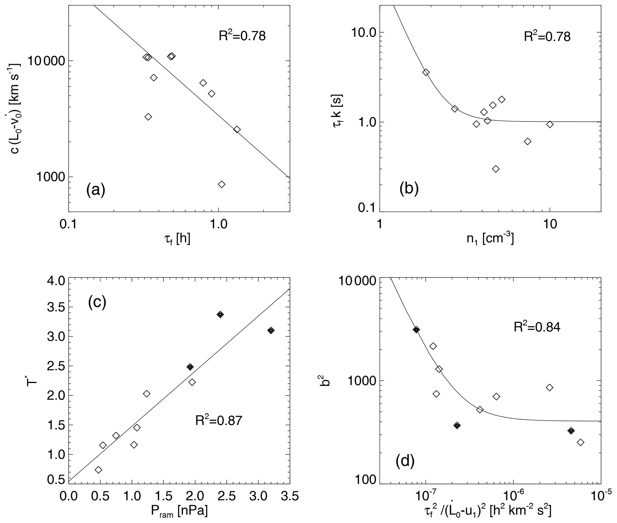
Figure 9 Empirical relations of free parameters and inputs. Open diamonds point out the data dispersion, the solid lines are the calculated regression tendencies, and we also present the squared correlation index between the data dispersion and the associated regression.

We show the results from our parametric exploration in the panels of Fig. 9. In panel (b) we plot (open diamonds) the product τ_f k as a function of the proton density of solar wind (n₁), which can be approximated by

$$\begin{array}{}\text{(19)}& k\left[{\displaystyle \frac{{\mathit{\tau }}_f}{\mathrm{1}\mathrm{h}}}\right]=\mathrm{58.4}{\left[{\displaystyle \frac{n_{\mathrm{1}}}{\mathrm{1}{\mathrm{cm}}^{-\mathrm{3}}}}\right]}^{-\mathrm{4.9}}+\mathrm{0.9}.\end{array}$$

This is also plotted in Fig. 9b as a solid line. According to Eq. (19), for a given τ_f, the CME radius is somehow inversely related to the solar wind density up to a limit value, after which it stays constant. This could be due to effects of solar wind inertia on the expansion of CMEs, since larger inertias (densities) of solar wind would evolve into slower expansion rates, which should lead to shorter radii of CMEs, consistent with Démoulin and Dasso (2009).

Concerning the temperature, we found that the value of T^* could be approximated by

$$\begin{array}{}\text{(20)}& T^{*}=\mathrm{1.5}\left[{\displaystyle \frac{P_{\mathrm{ram}}}{\mathrm{1}\mathrm{nPa}}}\right]+\mathrm{0.366},\end{array}$$

with $P_{\mathrm{ram}}=m_{\mathrm{p}}(\mathrm{1}+p_{\mathrm{2}}/p_{\mathrm{1}})p_{\mathrm{1}}$ the sum of ahead (p₁) and behind (p₂) ram pressure ($p=n{u}^{\mathrm{2}}/\mathrm{2}$) of solar wind (see the solid line in Fig. 9c). Equation (20) suggests that the more (less) compressed by the surrounding solar wind a CME is, the hotter (colder) than the average it would be. It is important to note that, when the effects of solar wind compression are negligible (p₂<p₁), the value of T^* could be satisfactorily approximated by solar wind (p₁) ahead solely, whereas, in the case of magnetic field intensity, we found that b² seems to be related to ${\mathit{\tau }}_f^{\mathrm{2}}/({\dot{L}}_{\mathrm{0}}-u_{\mathrm{1}})$ according to

$$\begin{array}{}\text{(21)}& \begin{array}{rl}{b}^{\mathrm{2}}& =\mathrm{6.72}\times {\mathrm{10}}^{-\mathrm{11}}{\left({\left[{\displaystyle \frac{{\dot{L}}_{\mathrm{0}}-u_{\mathrm{1}}}{\mathrm{1}\mathrm{km}{\mathrm{s}}^{-\mathrm{1}}}}\right]}^{\mathrm{2}}{\left[{\displaystyle \frac{{\mathit{\tau }}_f}{\mathrm{1}\mathrm{h}}}\right]}^{-\mathrm{2}}\right)}^{\mathrm{1.91}}\\ & +\mathrm{426.8}.\end{array}\end{array}$$

This relation is also plotted (solid line) in the panel. Thus, according to Eq. (21), we would expect stronger magnetic fields within fast CMEs related to solar flares of short duration. This relationship appears to have a lower limit when a slow CME is associated with a prolonged solar flare.

By combining Eq. (18) and the piston-shock model, Corona-Romero et al. (2017) were able to forecast travel times and arrival speeds and even to estimate masses of fast CMEs. Thus, it is reasonable to infer that Eqs. (19) to (21) could be a possible way to approximate the expected values of free parameters. In such a hypothetical case, those relationships would help to specify all the required data to calculate synthetic transits before an event impacts Earth; i.e., we could perform analytic forecasting of in situ transits of CMEs. Since once an event is identified by a coronagraph, it would be possible to collect the values of L₀, ${\dot{L}}_{\mathrm{0}}$, τ_f, n₁, and u₁, we would proceed to calculate the values of c, k, and b; and, by neglecting the effects of compression, we would approximate the value of T^*. Afterwards, with all those values known, we would apply our formalism to compute the in situ transit of the event as possibly would be seen at Earth's orbit.

To illustrate this, we “forecast” the synthetic profiles of Event 1. Figure 10 compares the results from this “forecasting” test (red profiles) and the already calculated synthetic transit of Event 1 (blue profiles). In general terms, we note in the figure that both profiles are close to each other, with the forecast profiles approximating their calculated counterparts. Additionally, we also note differences. For example, the “forecast” CME center (dashed red vertical lines) arrives a few hours earlier than the computed one, and the red profile of density is slightly above its blue counterpart, behaviors that suggest an excess of inertia. Regarding temperature and magnetic intensity forecast profiles, the main change we note is a translation caused by the early arrival noted above. Additionally, the “forecast” transit time (dotted red vertical lines) is significantly less than its calculated counterpart, which may imply faster bulk speed and/or a shorter radius. Here, it is important to highlight that the differences between the “forecast” and Table 2 values of the free parameters were 46.8 %, −8.6 %, 0.6 %, and 6.4 % for c, k, T^*, and b, respectively, values that explain the early arrival, the excess of density, the shorter transit time, as well as the similitude between temperatures and magnetic field intensities seen in the forecast profile.

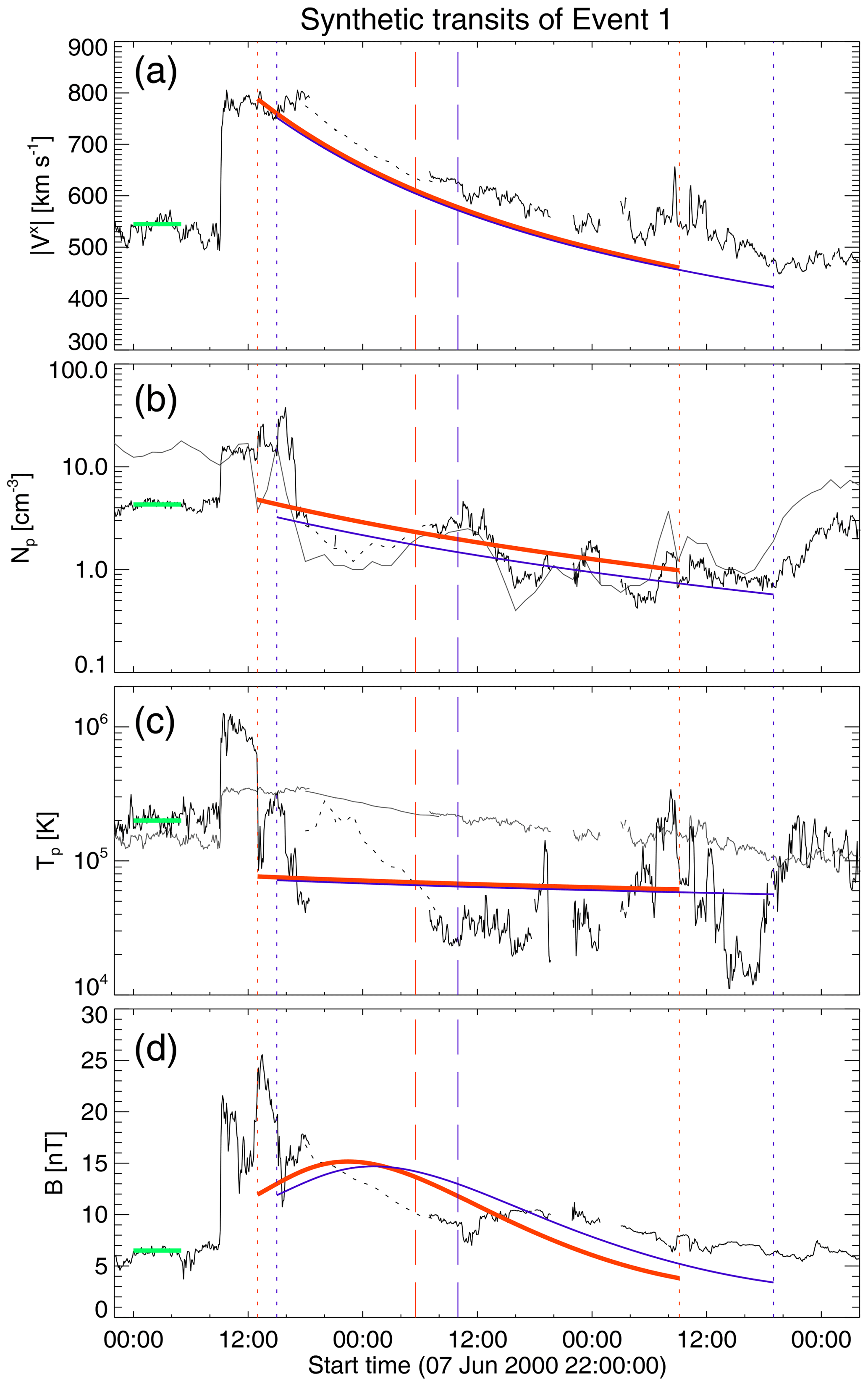
Figure 10 Synthetic transit profiles of Event 1 calculated for different values of free parameters. Panels (a), (b), (c), and (d) present the radial component of the solar wind speed ($\left|V^x\right|$), the density (N_p) and temperature (T_p) of protons and the magnetic field intensity (B), respectively. The red profiles were calculated with values of free parameters fixed by Eqs. (18) to (21), and the blue profiles are the same as shown in Fig. 4. Short-dashed and long-dashed vertical red lines mark the CME boundaries and center, respectively. Solid (dotted) black lines are 5 min (1 h) in situ measurements as extracted from NASA/GSFC's OMNI data set through the OMNIWeb service. Green solid lines mark in situ solar wind used for calculations (see Table 1). Solid grey lines in N_p and T_p panels are the plasma beta (10-fold) and the expected proton temperature (T_exp) (Lopez, 1987; Richardson and Cane, 1993, 1995), respectively. The free parameter values used to calculate the red synthetic transit were c=18.29, k=2.56, $T^{*}=\mathrm{2.16}$, and b=23.0.

Our formalism's forecasting capabilities tentatively rely on Eqs. (18) to (21). Corona-Romero et al. (2017) recently validated Eq. (18). If future studies validate the other remaining three, it would allow us to apply our formalism to systematic forecasting of CME arrivals. In addition, because our speed and magnetic profiles have lower errors, our work might also help to forecast CME geoeffectiveness, since the product v^x×B^z plays an important role for this purpose (see Richardson and Cane, 2011, and references therein). In such a case, our forecasting capabilities could be strengthened by combining our formalism with, for example, the approach of (Savani et al., 2015, 2017), which aims to forecast the magnetic polarity of flux ropes and their orientations. Furthermore, by combining our results with previous works Corona-Romero and Gonzalez-Esparza (e.g., 2016), we would be able to simultaneously forecast in situ transit profiles of CMEs and associated shocks/sheaths. The capability to simultaneously forecast in situ transits of CMEs, the geoeffectiveness, associated forward shocks, and plasma sheaths is of great interest for space weather purposes, since more intense geomagnetic storms are triggered by such phenomena (Ontiveros and Gonzalez-Esparza, 2010, and references therein). However, such a goal also requires additional information, such as the magnetic field within the sheath regions, which is not within the capabilities of such models yet. Nevertheless, if this formalism is shown to be robust under a range of conditions, it can lead to an important operational tool for space weather, particularly for those scenarios when the response time is of importance, such as early warning systems. Exploring its robustness would be our immediate task.

5 Conclusions

We presented a semi-empirical formalism to compute synthetic in situ transits of fast Earth-directed halo CMEs. Our formalism combines analytical and empirical models to develop a method based on simple equations that allows us to approximate the radial speed, density, and temperature of protons, and magnetic field intensity during the transit of CMEs as seen at the orbit of Earth. Although we compute synthetic transits for 1 AU, our equations can be adapted to other heliocentric distances like Mars or elsewhere. Additionally, our formalism also calculates the travel time of the CME center and its arrival speed as well.

To compute synthetic in situ transits of CMEs, we used data related to the event being analyzed. The data our method requires are (i) the initial position and speed of CMEs (from coronagraph images), (ii) the rise phase duration from the associated solar flare (taken from X-ray fluxes), and (iii) the solar wind conditions from in situ measurements. Additionally, the free parameters were associated with inertia, size, temperature, and magnetic field of CMEs, and we used them to tune our results.

We used our formalism to approximate 10 in situ transits of fast CMEs that occurred during 2000–2015 and found that profiles of speed, magnetic intensity, and temperature had average errors of 10 %, 27 %, and 83 %, respectively. Additionally, the error for the travel time of the CME center was 9 %. In the case of density, our results were strongly affected by the solar wind compression on CMEs, which caused discrepancies with the observations. In this sense, the average error of density for all events was 102 %, whereas, neglecting the three events significantly perturbed by the compression effects, the average error dropped to 46 %. It is important to remark that errors of temperature and density, even in those compressed cases, were lower than the rapid and large variations inherent in the in situ data.

In addition to computing in situ transits, we also found that deceleration of the CME expansion rate may play an important role in the way in situ transits are “seen”. On the one hand, stronger decelerations apparently provoke curved-like profiles in speed synthetic transits; this contrasts with constant-slope profiles of CMEs with an almost constant expansion rate. On the other hand, we noted that our calculated magnetic-intensity profiles tend to be symmetric (asymmetric) for CMEs with negligible (large) deceleration expansion rates. Surprisingly, those large and fast CMEs would tend to have larger deceleration expansion rates than those smaller and slower ones.

Our formalism relies on a number of assumptions that simplified the conditions in which a fast CME evolves and propagates. From these simplifications arose a number of limitations that may increase the error in our results, particularly for complex events. Nevertheless, our formalism proved to approximate particularly well the speed and magnetic intensity profiles, both directly related to the geoeffectiveness of CMEs. Besides, we found possible empirical relationships to estimate the free parameters our model requires, which might allow us to implement our method to forecast in situ transits of CMEs. Hence, in conjunction with other approaches, our model can lead to an important operational tool for space weather forecasting, especially in the case of early warning systems.