
the Creative Commons Attribution 4.0 License.
the Creative Commons Attribution 4.0 License.
 | 30 Sep 2026
Ionospheric currents and auroral signatures during successive earthward bursty bulk flows and dipolarization: a 7 December 2023 case study
Vanina Lanabere

Stephan Buchert
Adrian Blagau
Harriet George
Sota Nanjo
Liisa Juusola
Andrew P. Dimmock
Samuel Wharton
Heikki Vanhamäki
Octav Marghitu
Louis Richard
Alice V. L. Wallner
Daria Kotova
Theresa Hoppe
Jennifer A. Carter
Anita Aikio
Earthward bursty bulk flows (BBFs) in the central plasma sheet are frequently accompanied by dipolarization fronts, and together they account for a large fraction of the energy and momentum transported from the magnetotail to the high-latitude ionosphere through field-aligned currents (FACs). On 7 December 2023, between 18:00 and 22:00 UT, six BBFs-intervals were detected by THEMIS, with clear dipolarization signatures in the last four intervals. These flows map to the pre-midnight magnetic local time sector over northern Fennoscandia, where the ionospheric response is examined using horizontal equivalent current density derived from the IMAGE magnetometer network and auroral emissions from all-sky cameras. At the beginning of the interval, the ionospheric current system exhibits a stable Harang discontinuity, which becomes progressively distorted after each BBF and ultimately evolves into a clear westward electrojet. The first two dipolarizing intervals are accompanied by auroral pseudo-breakups, whereas the final two display an auroral breakup and poleward expansion characteristic of substorms. A key interval occurs during the fourth BBF, whose mapped footpoint intersects the Swarm A/C orbit and reveals a strongly localized pair of upward and downward FACs spanning 35–50 km in latitude, with the upward current colocated with a discrete auroral arc. Throughout the BBF activity, the horizontal ionospheric current density reorganizes rapidly around the mapped footpoints, and the auroral arc intensifies simultaneously with THEMIS enhancements of 9–20 keV electron fluxes. These observations demonstrate that localized magnetotail flows can drive fast, structured, and cumulative modifications of the ionospheric electrodynamics, emphasizing the importance of multi-point measurements for resolving the temporal evolution of magnetosphere–ionosphere coupling during BBFs.
- Article
(18301 KB) - Full-text XML
- BibTeX
- EndNote


Geomagnetic disturbances (GMDs) and auroral activity observed in the Earth’s ionosphere arise from the transfer of energy and momentum from the solar wind into the magnetosphere–ionosphere system. Through decades of observations and modeling, the magnetotail has been identified as the region where this energy is stored and later explosively released, defining the classical loading–unloading cycle of geomagnetic substorms. During this cycle, magnetic flux is accumulated in the tail during the growth phase, leading to progressive stretching of the magnetic field lines. At onset, this stored flux is rapidly released, with part of the energy ultimately dissipated in the ionosphere (e.g., Baker et al., 1997). This release is accompanied by a reconfiguration of the near-Earth magnetic field towards a more dipolar geometry (dipolarization) (Baumjohann et al., 1999), marking the start of the expansion phase (Merkin et al., 2019). This explosive energy release produces the characteristic auroral substorm brightening and poleward expansion originally identified by Akasofu (1964), together with sharp ground magnetic perturbations.
The current system established at the substorm onset, the substorm current wedge (SCW), was first formulated by McPherron et al. (1973). The cross-tail current partially diverts into the high-latitude ionosphere through a pair of field-aligned currents (FACs) flowing into the ionosphere on the dawn side and out on the dusk side (R1-sense). The FACs close via an enhanced westward electrojet (WEJ). More recently, Liu et al. (2015) presented magnetotail observations supporting the idea that the SCW may form from the collective action of multiple small-scale wedgelets, each generated by an individual dipolarization flux bundle (DFB) or its associated dipolarization front, as originally proposed by Birn and Hesse (2013, 2014). DFBs are observationally defined as transient magnetotail flux tubes with a significantly more dipolar northward magnetic field component Bz and reduced plasma density n compared to the surrounding plasma sheet (e.g., Liu et al., 2013). They arise when reconnection occurs on highly stretched tail magnetic field lines, and the newly reconnected flux tubes contract earthward under magnetic tension, releasing stored energy and accelerating plasma toward the inner magnetosphere. This relaxation produces fast earthward plasma jets known as bursty bulk flows (BBFs) (Baumjohann et al., 1990). In the wedgelet framework, each BBF or DFB acts as a localized generator of FACs and ionospheric current channels, and the superposition of many such elements can reproduce the large-scale magnetic signatures traditionally attributed to a single SCW (Panov et al., 2019). A broader overview of SCW formation, wedgelet structure, and their relation to BBFs and dipolarization fronts is provided by Kepko et al. (2015).
Auroral signatures associated with BBFs have been documented in several observational studies, including narrow auroral streamers and small auroral expansions or pseudo-breakup activations (Nakamura et al., 2001), as well as auroral activations at the poleward edge of an expanded auroral bulge (Borodkova et al., 2002). The pseudo-breakups or pseudo-substorms (e.g., Ohtani et al., 1993) share several morphological features with substorms, but they do not evolve into the large-scale poleward expansion and global current-system reconfiguration characteristic of a full substorm. Recent studies have emphasized that pseudo-breakups may represent an early stage in a continuum of magnetotail activity, where localized flow bursts and limited reconnection signatures precede the development of a full substorm onset (e.g., Fukui et al., 2020).
The most important space weather effects and impacts of substorms on technological systems at high latitudes are, as summarized by Buzulukova and Tsurutani (2022, and references therein): (1) Geomagnetically induced currents (GICs), driven by rapid variations in ionospheric currents; (2) Spacecraft surface charging and deep dielectric charging, driven by enhanced fluxes of 1–50 keV electrons in the geostationary region and by intense precipitation of energetic electrons in the auroral zone; and (3) Global Navigation Satellite System (GNSS) signal degradation and communication disruptions, driven by ionospheric density irregularities produced by precipitation of 0.1–100 keV electrons. In the particular case of GICs, recent studies suggest that isolated GMDs are often associated with BBFs, DFBs, or a combination of both. For example, Wei et al. (2021) and Zhang et al. (2026) examined the magnetosphere–ionosphere response during the 7 January 2015 storm using Cluster, Swarm, and ground magnetometer data. Cluster-4 observed multiple BBFs in the inner magnetosphere, while ground stations recorded strong ground magnetic variations over a broad region rather than forming a localized signature. Swarm A/C crossed the mapped Cluster-4 footprint and detected a similar up-down-up-down FAC pattern, supporting a conjugate link between the BBFs and the ionospheric current system. Engebretson et al. (2024) investigated large, isolated GMDs and their relationship to DFBs, finding that GMD onsets typically preceded DFB signatures by about 2 min, with peak disturbances nearly simultaneous. In two events where isolated DFBs were conjugate to large GMDs, the authors found a characteristic ionospheric response consisting of a localized, intense upward–downward FAC pair. Similarly, Ngwira et al. (2025) showed that an isolated substorm during the 20 December 2015 storm, associated with earthward flows detected by THEMIS, produced a sharply localized northwestward electrojet situated between upward and downward FACs.
Understanding how these transient tail flows relate to ionospheric currents, auroral structures, and ground magnetic variations is therefore essential for linking magnetotail dynamics to space weather effects at high latitudes. In this study, we conduct a detailed examination of a sequence of recurrent BBF events on 7 December 2023, each exhibiting distinct plasma and magnetic signatures, that produced isolated GMDs and auroral activity well before substorm onset. This multi-instrument analysis allows us to track changes in the ionospheric current system and auroral morphology throughout each BBF interval. In addition, Swarm observations of FACs reveal the evolution of both large-scale FAC regions and small-scale structures near the BBF footpoint. The solar wind conditions, magnetotail measurements, ionospheric FACs, ground magnetic field data, and auroral observations are described in Sect. 2. Section 3 provides an overview of the event, including the identification of the BBF intervals and the mapping of their ionospheric footpoints. In Sect. 4, we present the evolution of the horizontal ionospheric current density and the associated auroral response to the BBFs, while Sect. 5 offers a detailed analysis of the FACs during the BBF–Swarm conjunction. The summary and discussion are given in Sect. 6, and the conclusions are presented in Sect. 7.
2.1 Solar wind
We use solar wind observations from four different spacecraft. Three of them, ACE (McComas et al., 1998; Smith et al., 1998), Wind (Harten and Clark, 1995; Lepping et al., 1995; Ogilvie et al., 1995), and Deep Space Climate Observatory (DSCOVR) (Burt and Smith, 2012), are located near the first Sun-Earth Lagrange point (L1), approximately 230 Earth radii (RE) upstream of the Earth along the Sun-Earth line. All three missions provide magnetic field measurements from fluxgate magnetometers. Solar wind plasma measurements are obtained using different instruments: ACE employs an electrostatic analyzer, DSCOVR uses Faraday cups, and Wind has both types onboard. All solar wind datasets used in this study were downloaded from NASA’s CDAWeb archive. In addition, during the interval analyzed in this study, two of the five THEMIS probes (Angelopoulos, 2008), THEMIS-B and THEMIS-C, were in lunar orbit and located in the solar wind upstream of the Earth. Magnetic field measurements from these probes are also provided by fluxgate magnetometers. Figure 1a shows the spacecraft trajectories in GSE coordinates on 7 December 2023 between 12:00 and 22:00 UT.
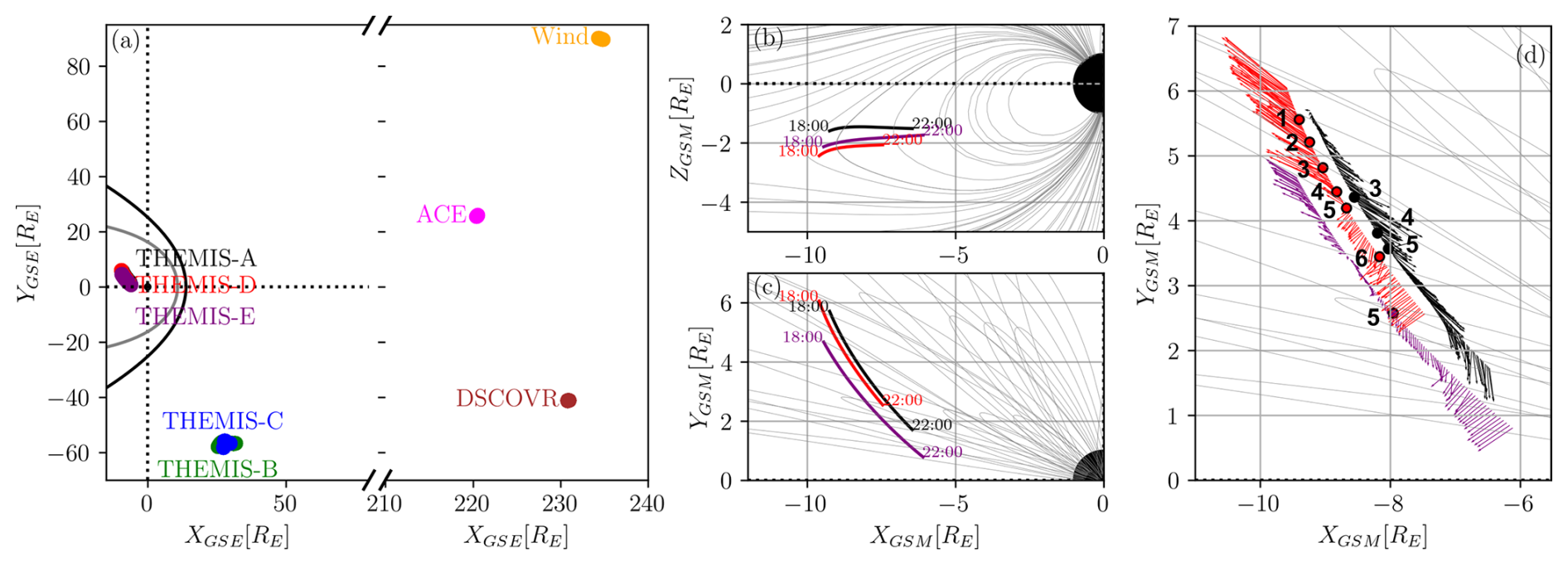
Figure 1(a) Orbits of Wind, ACE, DSCOVR, and THEMIS-B/-C in GSE coordinates on 7 December 2023 between 12:00 and 22:00 UT and THEMIS-A/-D/-E/ between 18:00 and 22:00 UT. The Earth's bow shock (black line) is estimated using the Farris and Russell (1994) model, and the magnetopause (gray line) is estimated using the Shue et al. (1998) model. (b–c) Orbits of THEMIS-A, THEMIS-D, and THEMIS-E in the XZ-GSM and XY-GSM planes on 7 December 2023 between 18:00 and 22:00 UT. The background magnetic field is computed using the Tsyganenko 89 model with a dipole tilt angle −16.4° and Kp=2.33, values that correspond to the conditions at 20:00 UT. (d) Zoom-in around THEMIS-A/-D/-E orbit together with the measured B field. The dots in panel (d) indicate the central times of the BBF detections in the George et al. (2026) database, with the number next to each dot identifying the corresponding BBF interval. The BBF observed during interval 5 was simultaneously detected by all three spacecraft.
2.2 Magnetotail
For the BBF observations, we use data from the THEMIS mission. During the interval examined here, THEMIS-A, THEMIS-D, and THEMIS-E were located in the near-Earth plasma sheet and provided closely spaced measurements, as shown in Fig. 1b, c. In addition to vector magnetic field data, thermal ion and electron velocity distributions from a few eV up to ∼30 keV are obtained from the Electrostatic Analyzer (ESA) (McFadden et al., 2008), and hot ions and electrons from 25 keV to >1 MeV are obtained from the solid state telescope (SST). Plasma bulk velocity and electron density are taken from the ground-calculated ESA + SST combined moments. All THEMIS datasets were accessed and processed using the pySPEDAS analysis framework (Grimes et al., 2022).
Figure 1d shows the observed magnetic field direction and magnitude in the GSM X-Y plane (arrows) for the three spacecraft. At the beginning of the interval, the observed magnetic at all three spacecraft agrees well with the external T89 model (Tsyganenko, 1989), shown as gray lines. Toward the end of the interval, however, the measured field develops a pronounced change in its direction, indicating a twisting or bending of the magnetic field lines. This reflects a significant departure from the nominal magnetospheric configuration given by the T89 model.
2.3 Ground-based measurements
Ground magnetic field measurements at 10 s resolution are obtained from the IMAGE (International Monitor for Auroral Geomagnetic Effects) magnetometer network (Tanskanen, 2009). These data are used to construct maps of ionospheric equivalent currents throughout the interval of interest. A subset of IMAGE stations also provides 1 s resolution data, which enable us to assess whether the FACs observed by Swarm produce detectable ground magnetic signatures at temporal scales below those resolved by the standard 10 s IMAGE network.
To characterize the global geomagnetic activity level, we use the Sym-H, AL, and AU indices (Iyemori et al., 1992; Davis and Sugiura, 1966). Sym-H provides a 1 min measure of the symmetric ring current, while AL reflects the intensity of the westward auroral electrojet and AU the eastward electrojet. In addition, we include the Hp30 index (Yamazaki et al., 2022), which offers a high-cadence (30 min) measure of global geomagnetic disturbances.
Auroral images were obtained from the all-sky camera (ASC) at Skibotn (SKB) Observatory. The system consisted of a Sony α6400 camera equipped with a MEIKE MK-6.5 mm F2.0 fisheye lens, operated at ISO 8000 with an exposure time of 8 s. Images were acquired every 30 s, using the same instrumental setup as described by Nanjo et al. (2025). The ASC in Kilpisjärvi (KIL) is an electron multiplying charged coupled device (EMCCD) camera. Images of the auroral green line (557.7 nm) are taken at least every 10 s with an exposure time of 0.8 s. More details about the camera setup are given by Sangalli et al. (2011). The images were projected onto a geographic grid assuming an emission altitude of 110 km and were used to examine auroral arc intensification and breakup in relation to the BBFs.
To assess the ionospheric impact of BBFs, we use Rate-Of-TEC-Index (ROTI) maps provided by the Norwegian Mapping Authority (NMA) through the European Space Agency (ESA) Space Situational Awareness (SSA) Space Weather Service Network. The ROTI product represents ionospheric irregularities mapped to a thin-shell ionosphere at 350 km altitude, and is derived primarily from the NMA GNSS network.
2.4 Ionosphere
The analysis of the FACs is carried out using data from the ESA's Swarm mission (Friis-Christensen et al., 2008). The constellation consists of three satellites (Alpha, Bravo, and Charlie), each equipped with a high-precision magnetic field payload composed of the Vector Field Magnetometer (VFM) and the Absolute Scalar Magnetometer (ASM). Swarm A and C fly side-by-side, and by the time of our analysis, their orbital altitude was approximately 480 km, consistent with the orbit-raising performed in 2023, with an east-west separation of 1.4° in longitude, and a maximum differential orbit delay of about 7 s on 7 December 2023. Swarm positions were mapped to 110 km altitude using the altitude-adjusted corrected geomagnetic (AACGM) coordinate system (Baker and Wing, 1989).
Single-spacecraft FAC product is derived from along-track variations in the magnetic field vector, providing an estimate of FAC density from a single orbital path. In addition to the single-spacecraft FAC product, we also employ the FAC densities along the orbit using the dual-satellite local least-squares (LLS) method estimates derived from the Swarm A–C pair (Vogt et al., 2013; Blagau and Vogt, 2019). Because the two satellites fly side-by-side, their combined measurements allow a more realistic estimation of the magnetic field gradient, which also includes the cross-track component. To minimize the influence of local fluctuation and fine tune the analysis to the spacecraft configuration, magnetic field data are prefiltered with a 20 s low-pass filter, thus providing reliable FAC estimations at spatial scales larger than approximately 150 km. The single- and dual-spacecraft FAC values used in this study were obtained using the SwarmFACE package (see Blagau and Vogt, 2023, for details).
To complement the single-spacecraft FAC product, we analyze the orientation and planarity of the current sheets using the multiscale minimum variance analysis (MS-MVA) technique developed by Bunescu et al. (2015, 2019); Bunescu (2024). MS-MVA provides eigenvalues and eigenvectors that describe the principal directions of magnetic field variation within a sliding analysis window. The MS-MVA analysis has been constrained to the plane perpendicular to the local magnetic field direction, which makes the third (minimum) eigenvalue always zero. The ratio of the maximum to intermediate eigenvalue quantifies the planarity of the FAC structure, with high values corresponding to highly planar structures. The partial derivative of the maximum/intermediate eigenvalue with respect to the analysis-window length provides proxies for the location and characteristic elongation of the FAC structures, indicated by the respective peaks in the derivatives. For sheet-like, planar and elongated FAC structures, the derivative of the intermediate eigenvalue is rather small and its accuracy likewise. For non-planar FAC structures, whose elongation is comparable (in order of magnitude sense) with the thickness, the information provided by the derivative of the intermediate eigenvalue is more reliable, though its quantitative relevance is still limited. The inclination angle describes the orientation of the FAC structure, as quantified by the intermediate variance eigenvector, with respect to the eastward direction in NEC (North-East-Center) coordinate system. An inclination of 90° corresponds to a north-south aligned FAC, while an inclination of 0° indicates an east-west aligned structure.
Horizontal ionospheric currents are analyzed using equivalent currents derived from ground-based magnetometer measurements from the IMAGE network. These are computed using the two-dimensional spherical elementary current systems (SECS) method (Amm, 1997; Amm and Viljanen, 1999; Juusola et al., 2016, 2020). In this approach, the measured magnetic field is decomposed into internal and external contributions associated with telluric currents and ionospheric/magnetospheric current systems, respectively. The SECS method represents these contributions using two equivalent current sheets: one at 1 m depth and one at an altitude of approximately 90 km. The external equivalent current system provides a two-dimensional, divergence-free (DF) approximation of the horizontal ionospheric current density, capturing the dominant part of the ground magnetic perturbations, while contributions from curl-free currents and associated FACs are negligible at ground level. In this study, ionospheric equivalent current density (JDF) derived from the SECS method is used to investigate the spatiotemporal evolution of electrojets over the Fennoscandian region at 10 s cadence.
On 7 December 2023 an isolated substorm event was detected by ground magnetometers. Figure 2 provides an overview of the event. Panels (a)–(c) show the solar wind conditions at L1 measured by ACE, and panels (d)–(f) the geomagnetic response at high latitudes (AL and AU indices), low latitudes (Sym-H index), and the planetary geomagnetic index Hp30. The yellow shaded interval (18:00–22:00 UT) marks the period during which six earthward BBFs were detected in the magnetotail. Although the solar wind data are not time-shifted to the bow shock, and therefore cannot be directly compared with the geomagnetic indices, two magnetic features may have acted as drivers or triggers of the sequence of BBFs that culminated in the final, larger substorm.
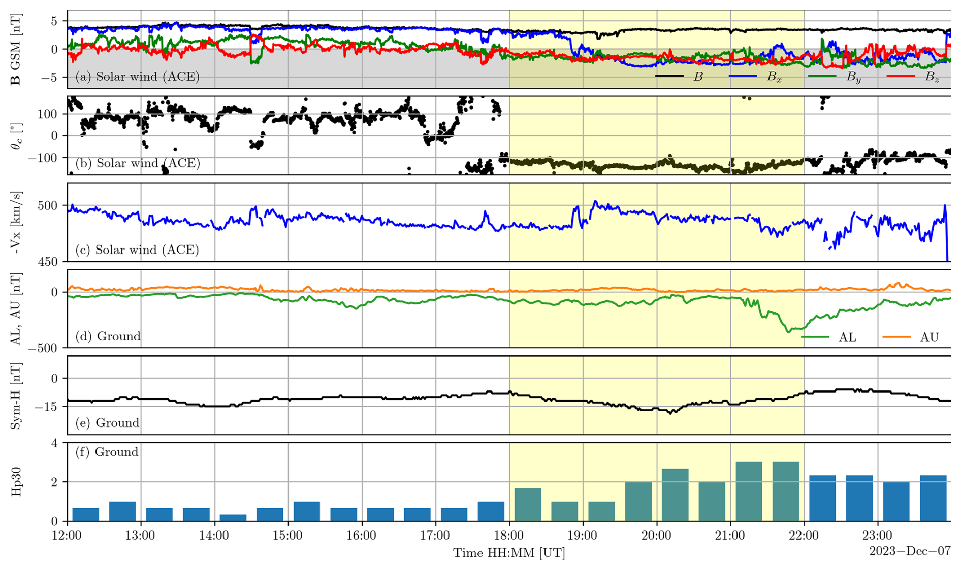
Figure 2Overview of the 7 December 2023 event between 12:00 and 23:59 UT. (a–c) Solar wind observations from ACE spacecraft (no time-shift): (a) interplanetary magnetic field components in GSM coordinates, (b) IMF clock angle, and (c) solar wind speed. (d–e) Ground geomagnetic response: auroral electrojet index AL (green) and AU (orange), and Sym-H index (black). (f) Hp30 geomagnetic index. The yellow shaded interval marks the period during which several earthward BBFs were detected in the magnetotail.
The first feature is an interplanetary magnetic field (IMF) Bx reversal: the IMF Bx component was strongly positive before 18:30 UT (), then reversed to Bx<0, and after 19:00 UT all three components became comparable in magnitude. The electron pitch-angle distributions measured by Wind (not shown) indicate that the strahl maintains the same 180° direction across the IMF rotation. This behavior suggests that the structure is consistent with a large-scale magnetic field inversion (Crooker et al., 2004) rather than a true polarity reversal or a closed magnetic loop. The second feature is a change in the IMF clock angle , around 18:00 UT as Bz turned negative after 17:30 UT and remained southward for the rest of the day.
These magnetic features, particularly the IMF Bx reversal, are observed consistently by all three spacecraft at L1 and by THEMIS-B and THEMIS-C in lunar orbit. Wind is the first to detect the IMF Bx change, at approximately 18:00 UT. To quantify the relative timing of this transition across the different spacecrafts, we time-shift the Bx measurements from each spacecraft and compute their linear correlation with the Wind Bx profile. The time lag corresponding to the maximum correlation is then taken as the propagation delay of the Bx reversal at each spacecraft relative to Wind. ACE observes the change 51 min later (correlation = 0.82), DSCOVR observes it 1 h 45 min later (correlation = 0.94), and THEMIS-B/-C observes it 2 h 56 min later (correlation = 0.96). Although all spacecraft observed the same structure, the propagated delays reported by OMNI vary between approximately 30 and 60 min, with a root mean square of about 15 min. This large and highly variable timing uncertainty occurs precisely between 18:30 and 20:00 UT, when the two IMF features are observed. For this reason, we do not apply the standard OMNI bow-shock-nose time shift in this study. However, our conclusions do not depend on accurately identifying the external driver or its exact timing.
A ground geomagnetic disturbance is clearly present at high latitudes, where the AL index shows a ∼300 nT decrease between 21:08 and 21:47 UT, characteristic of a substorm expansion phase. Throughout the interval, the Sym-H index remains mildly negative (approximately −10 nT), consistent with the late recovery phase of preceding geomagnetic activity. This activity included a geomagnetic storm on 1 December 2023 driven by a CME, which reduced Sym-H to −132 nT, followed by the arrival of a high-speed solar wind stream on 3 December and a second CME on 4 December (Temmer et al., 2025). The high-speed stream continued to influence the magnetosphere until 6 December, after which the system gradually transitioned into a rarefaction interval in the wake of the fast stream. Notably, Sym-H exhibits a gradual increase from 20:15 to 22:45 UT. Under stable solar-wind conditions, such an increase has been attributed by Huang et al. (2004) to magnetospheric dipolarization. Finally, the global geomagnetic index Hp30 in panel (e) shows an increase in geomagnetic activity from 19:30 UT with a maximum of 3.33 between 21:00 and 22:00 UT around the time of the substorm.
3.1 BBF intervals
Between 18:00 and 22:00 UT on 7 December 2023, several BBFs were detected by the THEMIS spacecrafts. Figure 3 shows six intervals during which the spacecrafts identified BBFs using the algorithm of George et al. (2026), indicated by the black, red, and purple shaded regions for the BBFs detected by THEMIS-A, -D, -E, respectively. In addition, three BBFs were identified in THEMIS-D using the Feng et al. (2025) algorithm, highlighted in cyan.
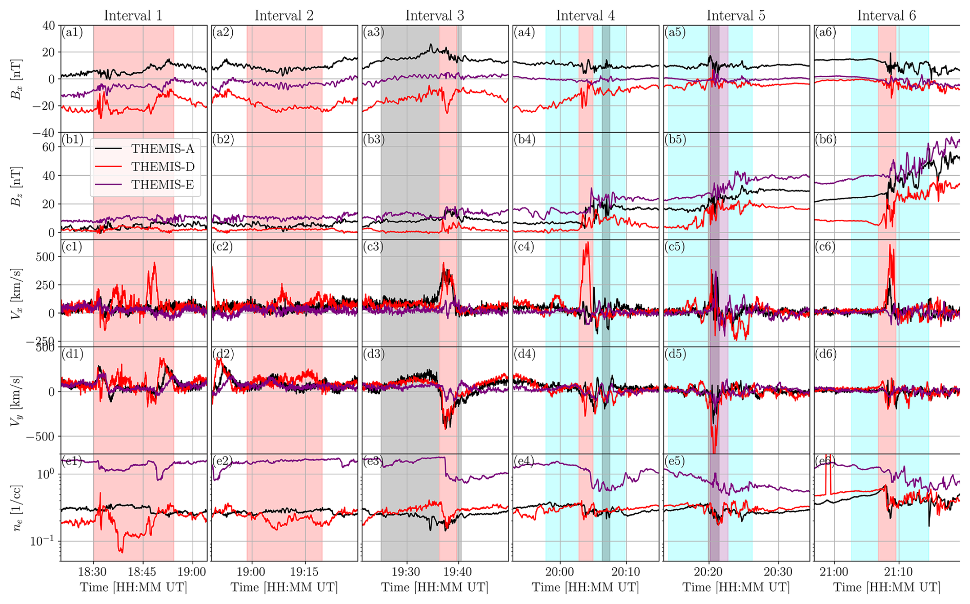
Figure 3Observations from THEMIS-A, -D, and -E during six BBF intervals presented by black, red, and purple lines, respectively. Panels show magnetic field components (a) Bx and (b) Bz in GSM, and ion velocity components (c) Vx and (d) Vy in GSM. Panel (e) presents electron density. The black/red/purple shaded intervals correspond to Earthward BBFs listed in the George et al. (2026) catalog detected by THEMIS-A/-D/-E, respectively, while the cyan intervals indicate BBFs in Feng et al. (2025) catalog detected by THEMIS-D.
In Fig. 3, panels (a) and (b) show the magnetic field components Bx and Bz in GSM coordinates. The Bx component provides information about the spacecraft position relative to the central plasma sheet. Throughout the intervals, Bx<0 for THEMIS-D, is close to zero for THEMIS-E, and is positive for THEMIS-A. This configuration indicates that THEMIS-E is located near the center of the plasma sheet, while THEMIS-A and THEMIS-D are positioned above and below it, respectively, consistent with the spacecraft geometry shown in Fig. 1b. The Bz component is used to identify dipolarization. All three spacecraft observe a gradual increase in Bz over time, with the sharpest enhancements occurring during the BBF intervals identified in the velocity profiles in panel (c). It is also interesting to note that there is an order in which the dipolarization signatures are observed by the satellites during the last three intervals: first THEMIS-D, then THEMIS-A, and last THEMIS-E. Based on the formation of the spacecrafts, this indicates an earthward dipolarization front.
In several cases, the BBFs are accompanied by strong Vy flows, as seen in panel (d). In particular, during Intervals 3 and 5 the Vy component is negative, indicating a dawnward flow deflection coincident with a radially earthward plasma motion. Notably, By in Fig. 1d shows an important change in its direction when the BBF is observed during Interval 5, probably associated with a twisting/bending of the magnetotail field lines due to Vy flow.
Panel (e) shows the electron density, where THEMIS-E exhibits the highest values, approximately an order of magnitude larger than those observed by THEMIS-A and THEMIS-D, consistent with its location in the central plasma sheet. During the BBFs intervals, THEMIS-D shows a decrease in electron density, and similarly for THEMIS-A and THEMIS-E, except during interval 2.
3.2 BBF ionospheric footpoint and Swarm Conjunction
During the interval when THEMIS-D observed the six BBFs, the spacecraft’s mapped footpoint at an altitude of 110 km was located in northern Fennoscandia and in the pre-midnight magnetic local time sector. We also looked at SuperDARN data (Chisham et al., 2007; Nishitani et al., 2019) (not shown), which indicates a predominantly twin-cell convection pattern. Between 18:00 and 19:30 UT, the plasma flow is westward at the top of Scandinavia. After 20:00 UT, Scandinavia moves into the region where the antisunward flow across the polar cap starts to move into return flows, resulting in some equatorward and eastward flow in our region of interest.
Figure 4a shows the THEMIS-A/-D/-E ionospheric footpoints computed with the T89 model for two geomagnetic activity levels. The lowest activity case (Hp30 = 1.33), representative of conditions between 18:30 and 19:30 UT, and the highest activity case (Hp30 = 3.33), corresponding to the interval between 21:00 and 22:00 UT. Swarm A and C (blue and light blue lines, respectively) intersect the THEMIS footpoint twice. The first conjunction occurs between 18:28 and 18:31 UT, when Swarm crosses all three THEMIS mapped footpoints. This crossing coincides with the first BBF interval observed by THEMIS-D (18:30–18:50 UT). The second conjunction occurs approximately 90 min later, between 20:02 and 20:05 UT, during Interval 4, when THEMIS-D detected another BBF between 20:02:50 and 20:04:58 UT. The central time of each BBF is mapped to an altitude of 110 km using several Tsyganenko magnetic field models (T89, T96, T01, T04). We then estimate a representative BBF footpoint by computing the spherical geometric median of the model-dependent footpoints. This centroid (shown as red stars) corresponds to the location on Earth’s surface that minimizes the sum of geographic distances to all model estimates. At the time of the BBF–Swarm conjunction, the centroid for Interval 4 maps to 69.62° N, 26.4° E, located eastward of the Swarm A track at 20:03:37 UT (69.6° N, 22.1° E).
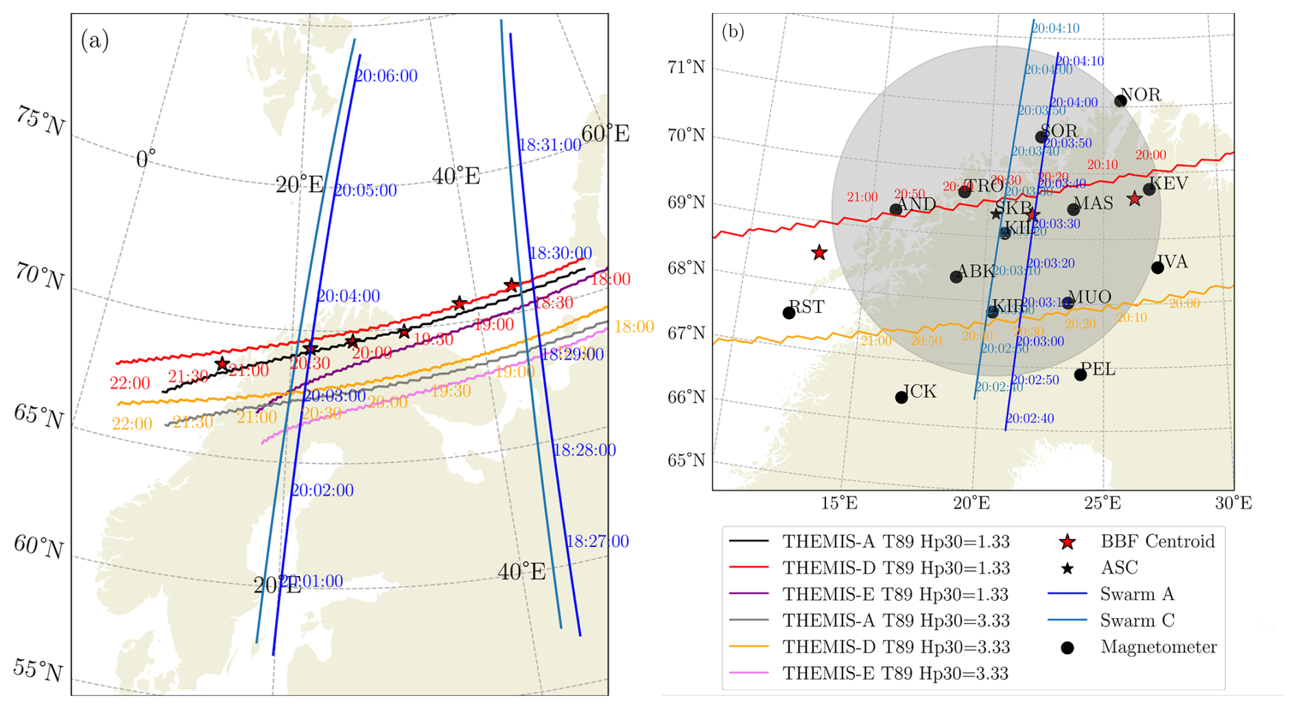
Figure 4Ionospheric footpoint on 7 December 2023 between 18:00 and 22:00 UT. (a) THEMIS-A/-D/-E orbit using the T89 model for Kp = 1.33 in black, red, and purple respectively, and for Kp = 3.33 in grey, orange, and pink respectively. Ionospheric centroid footpoint of the BBFs detected by THEMIS-D (red stars) together with THEMIS orbit mapped to the ionosphere using the Tsyganenko 89 model, and the Swarm A (blue) and Swarm C (light blue) orbits. All BBF centroids, THEMIS and Swarm orbits are mapped to 110 km altitude. (b) Zoom-in on northern Fennoscandia showing the last three THEMIS-D BBFs footpoints together with the locations of 14 IMAGE magnetometers around the BBF-Swarm conjunction location (black dots). The Skibotn ASC is indicated with a black star, and its projection at 110 km altitude for a 20° elevation angle is shown as the grey circular area.
A zoom-in around the BBF–Swarm conjunction during Interval 4 is shown in panel (b). For the last three BBF events, the mapped BBF ionospheric footpoints also include the TA15b and TA15n Tsyganenko models, plotted together with the earlier versions in different colors. The largest difference between models for each BBF event is about 5–6° in longitude (corresponding to 3.2–4° magnetic longitude) and from 1.6 to 2.8° in latitude (i.e., 1.7–3.2° magnetic latitude). This spread in the mapped BBF location is nevertheless smaller than that reported by Lanabere et al. (2025), primarily because the BBFs examined here occur closer to Earth (6–10RE) than those observed by MMS spacecraft. However, the increase in latitudinal spread with geomagnetic activity is consistent with the relationship reported in that study. The estimated BBF ionospheric footpoint centroids are taken as our best approximation of the true ionospheric footpoint of the BBFs. While the magnetotail magnetic field observations align well with the T89 model during the first four intervals, the last two intervals exhibit substantial distortions of the field geometry, thereby increasing the uncertainty in the mapped BBF ionospheric footpoint locations even under relatively quiet geomagnetic conditions.
Ground magnetometer stations from the IMAGE network are shown as black dots along the THEMIS-D and Swarm A/C trajectories. Notably, KIR, KIL, and SOR lie along or between the Swarm A/C passes, providing excellent ground-based coverage of the conjunction region. Five all-sky cameras were operating in the area: Tromsø (TRO), Skibotn (SKB), Abisko (ABK), Kilpisjärvi (KIL), and Kiruna (KIR). Only SKB and KIL images are shown, as Kiruna was cloud-covered, the TRO observations were nearly identical to those from SKB, and ABK is far south from the main auroral activity.
In this section, we examine the spatial and temporal evolution of the horizontal ionospheric currents using the ionospheric equivalent current over Fennoscandia, covering the region from 4–36° E and 54–79° N. Only the BBFs observed during Intervals 3–6 map into this domain and are analyzed in detail. For each interval, a longitudinal cut along the BBF footpoint longitude is used to construct a keogram showing the time evolution of the ionospheric currents density. Finally, the auroral activity for each interval is shown using images from the Skibotn ASC. The complete time evolution between 18:00 and 22:00 UT of the maps shown below, together with THEMIS-D observations of Vx, Bz, and electron flux, is available in the Video supplement.
4.1 Interval 3
Figure 5 shows the horizontal ionospheric equivalent current density JDF and auroral activity during the BBF and dipolarization observed by THEMIS-D in Interval 3 between 19:30 and 19:45 UT. Panels (a1)–(a4) show the ionospheric equivalent current magnitude and direction JDF (arrows), together with regions of clockwise (blue-shaded) and counterclockwise (red-shaded) vorticity (∇×JDF)z over Fennoscandia at four selected times. Clockwise vorticity is typically associated with downward FACs, while counterclockwise vorticity corresponds to upward FACs under the conditions outlined in Juusola et al. (2009, 2023). The BBF footpoint centroid is marked with the red star, and the BBF footpoints estimated from the Tsyganenko models are shown as colored dots: T89 (red), T96 (orange), T01 (green), T04 (yellow), TA15n (purple), and TA15b (magenta). Panels (b1)–(b4) show four snapshots from the Skibotn ASC images projected at 110 km altitude, where clockwise and counterclockwise JDF vorticity are indicated with solid and dashed lines, respectively. The snapshot times are marked by vertical black lines in panel (c). Panel (c) shows the keogram of JDF along the BBF longitude together with the THEMIS-D Vx measurements in the magnetotail.
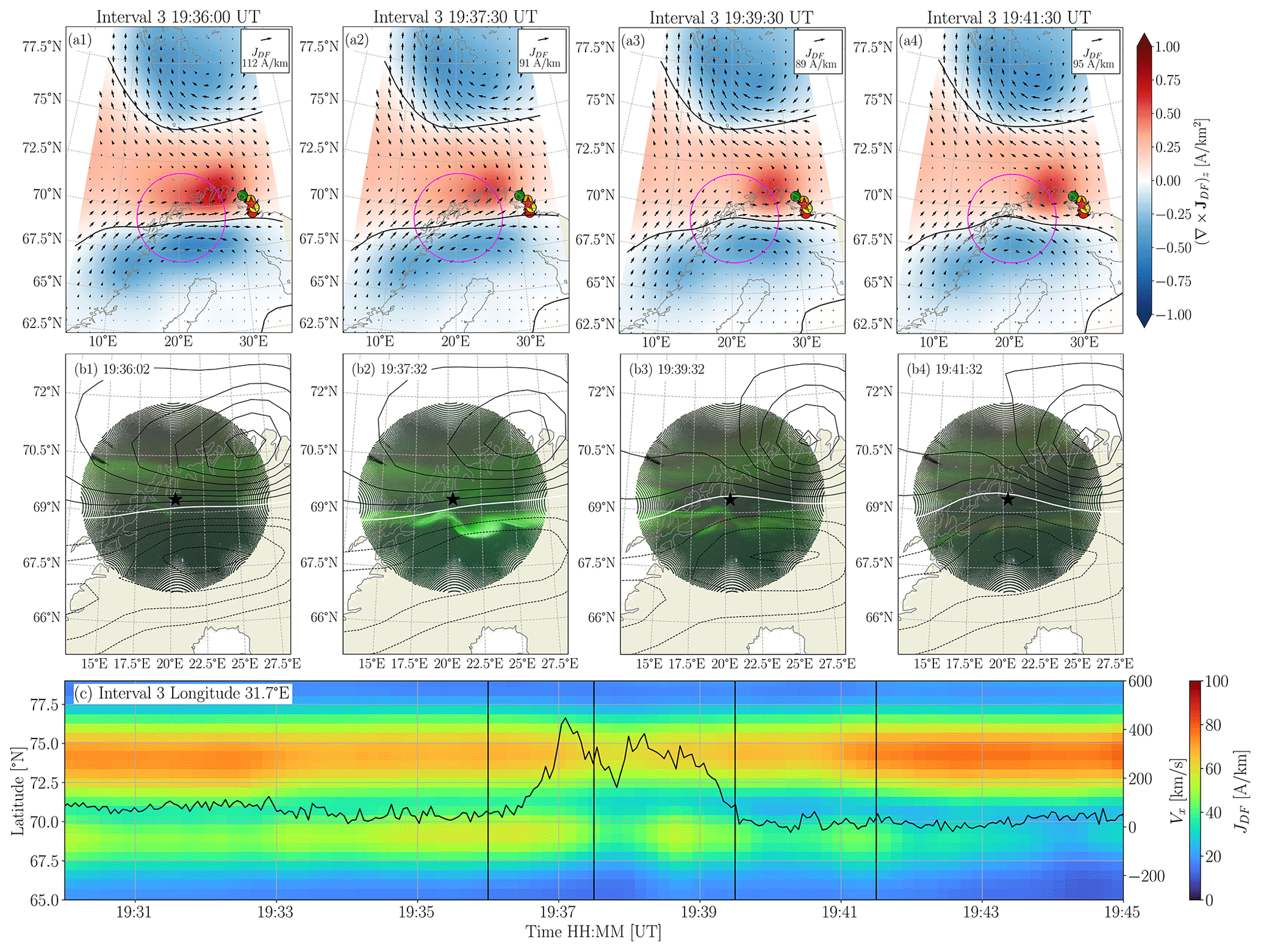
Figure 5Ionospheric horizontal current density and auroral activity on 7 December 2023 between 19:30 and 19:45 UT, including Interval 3. (a) Ionospheric equivalent current map magnitude and direction JDF (arrows), and its vorticity (∇×JDF)z (shaded). (b) Skibotn ASC images projected at 110 km, clockwise/counterclockwise JDF vorticity in solid/dashed lines. The null vorticity value is shown in a solid line. The star indicates the ASC location. (c) Keogram of JDF along the BBF ionospheric footpoint longitude together with the THEMIS-D Vx observations. The vertical black lines indicate the four snapshot times. The magenta circle in panels (a) indicates the ASC field-of-view projected at 110 km altitude. The red star marks the BBF footpoint centroid computed from the Tsyganenko models, shown in dots: T89 (red), T96 (orange), T01 (green), and T04 (yellow).
The map in panel (a1) reveals an eastward electrojet centered near 68° N and a northwestward current system near 75° N. These two systems are connected by a northward current, strongest at the eastern flank of the eastward current. The reversal between eastward and westward currents, together with the northward turning, is characteristic of the Harang discontinuity (Koskinen and Pulkkinen, 1995).
At the time when the BBF is detected in the magnetotail, the BBF footpoint lies on the eastern side of the eastward electrojet, within the region of counterclockwise vorticity where the current turns northward. The current directions show no significant reorientation, panel (a2), although the current magnitudes are affected, particularly within the eastward current, as seen in the keogram in panel (c). Even though the Skibotn ASC field-of-view does not include the BBF ionospheric footpoint centroid, an auroral arc brightens at the time of the BBF detection, panel (b2). Soon after the BBF, the auroral arc rapidly fades, while the eastward current weakens and the westward current strengthens relative to the pre-BBF interval.
4.2 Interval 4
Figure 6 shows the horizontal ionospheric current density, auroral activity, and magnetotail observations between 20:00 and 20:15 UT in the same format as Fig. 5. At the beginning of the interval, the horizontal current system displays a Harang discontinuity configuration (see Video supplement), similar to that in Fig. 5a4, and the eastward electrojet begins to weaken rapidly around 20:00 UT. The map in panel (a1), and the keogram in panel (c) show that the horizontal currents are dominated by a WEJ near 75° N and a weaker eastward component around 69° N. These two systems are connected by a counterclockwise vortex. The Skibotn auroral images show an auroral arc located close to the two oppositely rotating vortices, as shown in panel (b1).
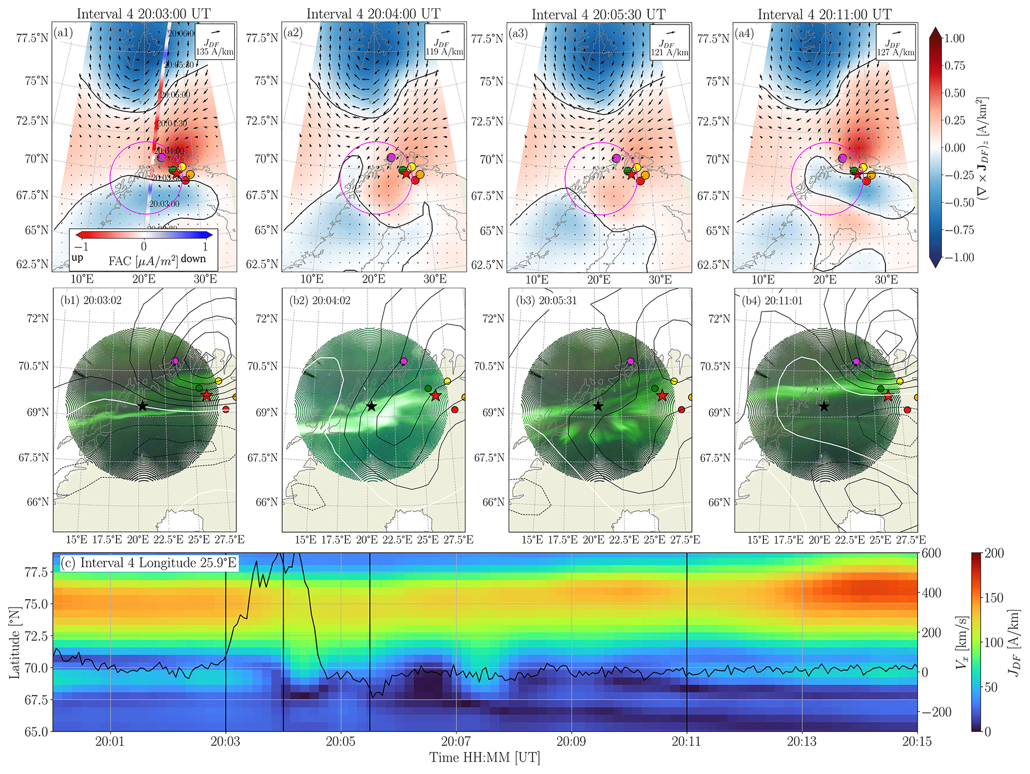
Figure 6The same as Fig. 5 except for the Interval 4 on 7 December 2023 between 20:00 and 20:15 UT. Panel (a) at 20:03:00 UT includes the Swarm dual spacecraft FACs projected at 110 km altitude. The BBF footpoint centroid and the ASC are displayed as a red and a black star respectively. The BBF footpoint centroid computed from the Tsyganenko models are shown in dots: T89 (red), T96 (orange), T01 (green), and T04 (yellow), TA15n (purple), and TA15b (magenta).
A BBF is observed when Vx exceeds 150 km s−1 between 20:03:05 and 20:04:32 UT. Around this time, between approximately 20:03:20 and 20:04:10 UT in panel (a2), a rapid reconfiguration of the horizontal currents occurs around the BBF footpoint location. During this period, the counterclockwise vortex shifts equatorward, bringing the BBF footpoint directly into the region of counterclockwise vorticity, as shown in panel (a3). The strength of the vortex fluctuates between 20:04 and 20:08 UT, consistent with the variations shown in the keogram.
Approximately one minute later, the arc intensifies and expands both poleward and equatorward (panel b2 and b3), coinciding with the intensification and equatorward motion of the pre-existing counterclockwise vortex.
After 20:08 UT, the pre-BBF eastward current re-establishes, but the large-scale current pattern no longer resembles the Harang discontinuity. Instead of the dominant northward current on the eastern side during the Harang configuration, the system now exhibits an equatorward current on the western flank of the counterclockwise vortex, as shown in panel (a4).
By the end of the interval in panel (b4), when the eastward current re-establishes, a stable auroral arc is again located between the two opposite-sense vortices (or within the eastward horizontal current), positioned slightly farther north than before the BBF arrival.
Between 20:03 and 20:04 UT, the Swarm A and Swarm C spacecraft cross close to the mapped BBF footpoint, providing valuable information on the FACs distribution. The dual-spacecraft FAC estimates resolve structures larger than ∼150 km, while smaller-scale features are captured by the single-spacecraft FACs discussed later in Sect. 5. In general, downward FACs (blue dots) coincide with regions of clockwise vorticity (blue shade), whereas upward FACs (red dots) align with regions of counterclockwise vorticity (red shade). A mismatch is observed between 75 and 77.5° N, likely due to the limited magnetometer coverage available for constructing the JDF maps in this latitude range. The BBF footpoint lies between the southernmost pair of upward and downward FACs, that is, between the two oppositely rotating vortices.
4.3 Interval 5
The fifth BBF is detected roughly 10 min after the previous one. At the beginning of the interval, the ionospheric configuration closely resembles the end of Interval 4 as illustrated in Fig. 7. A strong WEJ is present near 75° N, from which an equatorward current extends and forms two vortices of opposite sense: a counterclockwise vortex to the northeast and a clockwise vortex to the southwest, with a weak eastward current in between. During this interval, the magnetic field lines observed by THEMIS-D and THEMIS-E exhibit clear signatures of twisting or bending, indicating significant magnetotail reconfiguration. The ASC image in panel (b1) shows that at the beginning of the interval, an auroral arc is located north of Skibotn. This arc remains fairly stationary from its first appearance around 20:05:31 UT (during Interval 4) until approximately 20:16:31 UT.
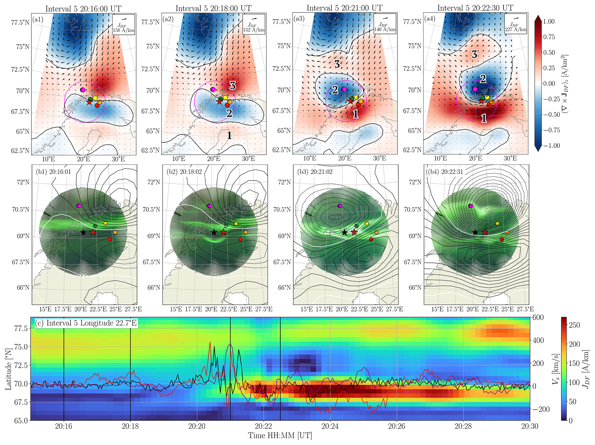
Figure 7The same as Fig. 5 except for the Interval 5 on 7 December 2023 between 20:15 and 20:30 UT. Panel (c) shows measurements done by THEMIS-A (black), THEMIS-D (red), and THEMIS-E (purple).
Between 20:16 and 20:19 UT THEMIS-D observes two intervals of Vx>0, followed by an interval of Vx<0 flux, all peaking near 100 km s−1. Between 20:20:00 and 20:21:30 UT, all three THEMIS spacecraft detect earthward flows with Vx>200 km s−1, alternating with short intervals of tailward flows. Around this time, a new WEJ forms near 70° N (panel a3), replacing the dominant eastward current present in panels (a1)–(a2). This newly intensified westward current places the mapped BBF footpoint within a region of counterclockwise vorticity, indicating a direct ionospheric response to the flow arrival. The numbers in panels (a) are included to track the displacement of the main vorticity regions throughout the interval. The ASC image shows a new arc forming equatorward (panel b2), and a pronounced brightening occurs at 20:21:02 UT (panel b3), coincident with the sudden intensification of the newly formed WEJ.
The last two snapshots in panels (a3)–(a4), together with the keogram in panel (c), show a highly dynamic WEJ associated with the evolution of vortices 1 and 2. In panel (c), the total current magnitude JDF indicates that the equatorward WEJ begins to intensify around 20:20:00 UT, increasing rapidly in both strength and latitudinal extent until approximately 20:22:00 UT. After this peak, the current weakens slightly and contracts until about 20:22:30 UT, when a second enhancement begins. This second intensification is stronger and broader than the first, reaching its maximum around 20:24:00 UT. During this time, the ASC image shows a sudden brightening (panel b3), followed by auroral breakup and polar expansion of the aurora arc (panel b4). By the end of the interval, two strong WEJs are visible: the original poleward WEJ and a newly formed equatorward WEJ. These two jets are separated by a narrow region of very weak magnetic field, with the equatorward WEJ becoming the stronger of the two.
Between 20:30 and 21:00 UT, during the recovery phase of the substorm, the horizontal currents undergo a sequence of changes in structure, location, and magnitude, eventually settling into a pattern similar to that observed in Interval 3, characteristic of the Harang region. This evolution will be discussed in more detail in the Discussion section.
4.4 Interval 6
Finally, we describe the last interval, which culminates in a stronger substorm than the one in Interval 5, and corresponds to the final enhancement of auroral activity observed that day, as shown in Fig. 8.
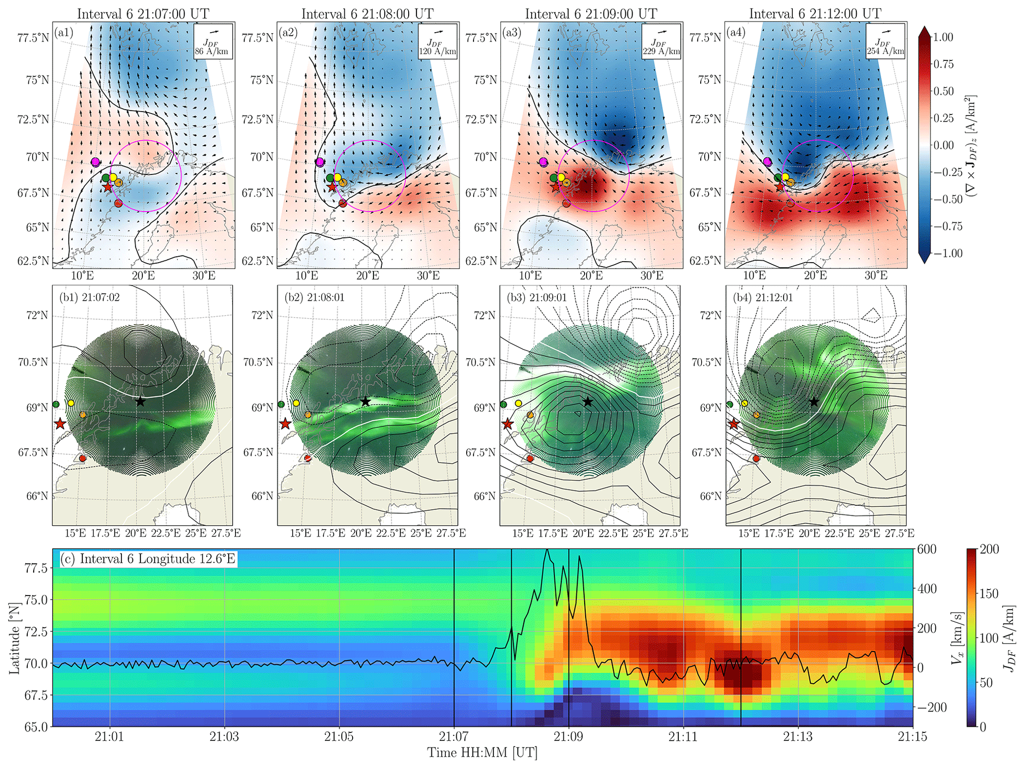
Figure 8The same as Fig. 5 except for the Interval 6 on 7 December 2023 between 21:00 and 21:15 UT.
After the substorm in Interval 5, both the auroral activity and the ionospheric currents return to a configuration characteristic of the Harang region. In this interval, however, the maximum eastward and westward currents are displaced westward compared to Interval 3. This configuration, as shown in panel (c) remains stable until around 21:06 UT.
The THEMIS observations reveal that the BBF begins a progressive acceleration around 21:07 UT, remaining above 150 km s−1 from 21:08:07 to 21:09:17 UT and reaching a peak velocity of 605.5 km s−1 at 21:08:37 UT. Panels (a2)–(a3) shows that the BBF maps in the region with large changes in the currents. Around this time, the newly formed vortex near the BBF footpoint intensifies rapidly between 21:07:20 and 21:08:40 UT, producing a strong WEJ on the eastern side of Fennoscandia, initially located far to the east of the BBF footpoint.
The WEJ then expands in longitude and subsequently broadens in latitude, forming a very strong and wide dominant westward current system (panel a3). At this stage, the BBF footpoint lies within the WEJ channel. Following this, the WEJ shifts poleward, reaching its most poleward position at 21:09:30 UT. By 21:10:50 UT, the electrojet expands equatorward, as well as longitudinally, followed by successive shifts and magnitude variations, as seen in the JDF keogram in panel (c).
Even though the BBF footpoint falls outside the ASC field-of-view projected at 110 km, the auroral evolution mirrors these magnetotail signatures with remarkable precision (panels b). At 21:05:32 UT, an auroral arc appears well south of Skibotn and intensifies by 21:07:02 UT. By 21:07:32 UT, the arc bifurcates, and the newly formed poleward structure brightens rapidly and moves northward, reaching its maximum intensity and poleward extent at 21:09:01 UT. Shortly after, at 21:09:31 UT, the aurora breaks up, and multiple structures drift southwestward.
The JDF maps in panels (a) and keogram in panel (c) show a tightly coupled response. The poleward migration of the bifurcated aurora coincides with the formation and intensification of the equatorward WEJ. As the aurora moves poleward, the WEJ also shifts poleward. The auroral breakup aligns with the moment when the WEJ expands both poleward and equatorward, and the drifting auroral structures toward the southwest occur during intervals of enhanced equatorward WEJ activity. The relation between the BBF footpoint in the evolution of the horizontal currents remains consistent with that described in the previous intervals, with the BBF footpoint located within the region where the new counterclockwise vortex emerges.
A zoom-in view of the ionospheric horizontal current density, the FACs estimated from Swarm A/C, and the auroral images from the Kilpisjärvi (KIL) station is shown between 20:03:07 and 20:04:00 UT in Fig. 9. The Swarm data is identical in all subplots but is overlaid against the JDF and the auroral images to contextualize the FACs. We use auroral images from the KIL all-sky camera instead of SKB because KIL provides higher temporal cadence and is located closer to the region where Swarm observes the strong upward–downward FAC pair. Both Swarm and aurora images are projected to 110 km. Panels (c)–(e) present the corresponding time series from the ground magnetometers shown in Fig. 9a. All curves show the magnetic field variations (ΔB) in the north (X), east (Y), and downward (Z) components relative to the values observed at 20:01:00 UT. Among these stations, KIR, KIL, and SOR (ordered from lower to higher latitude) lie closest to the Swarm track as the spacecraft moves from south to north in ascending orbit. Swarm A/C position at each snapshot is indicated with the green/magenta arrow, respectively.
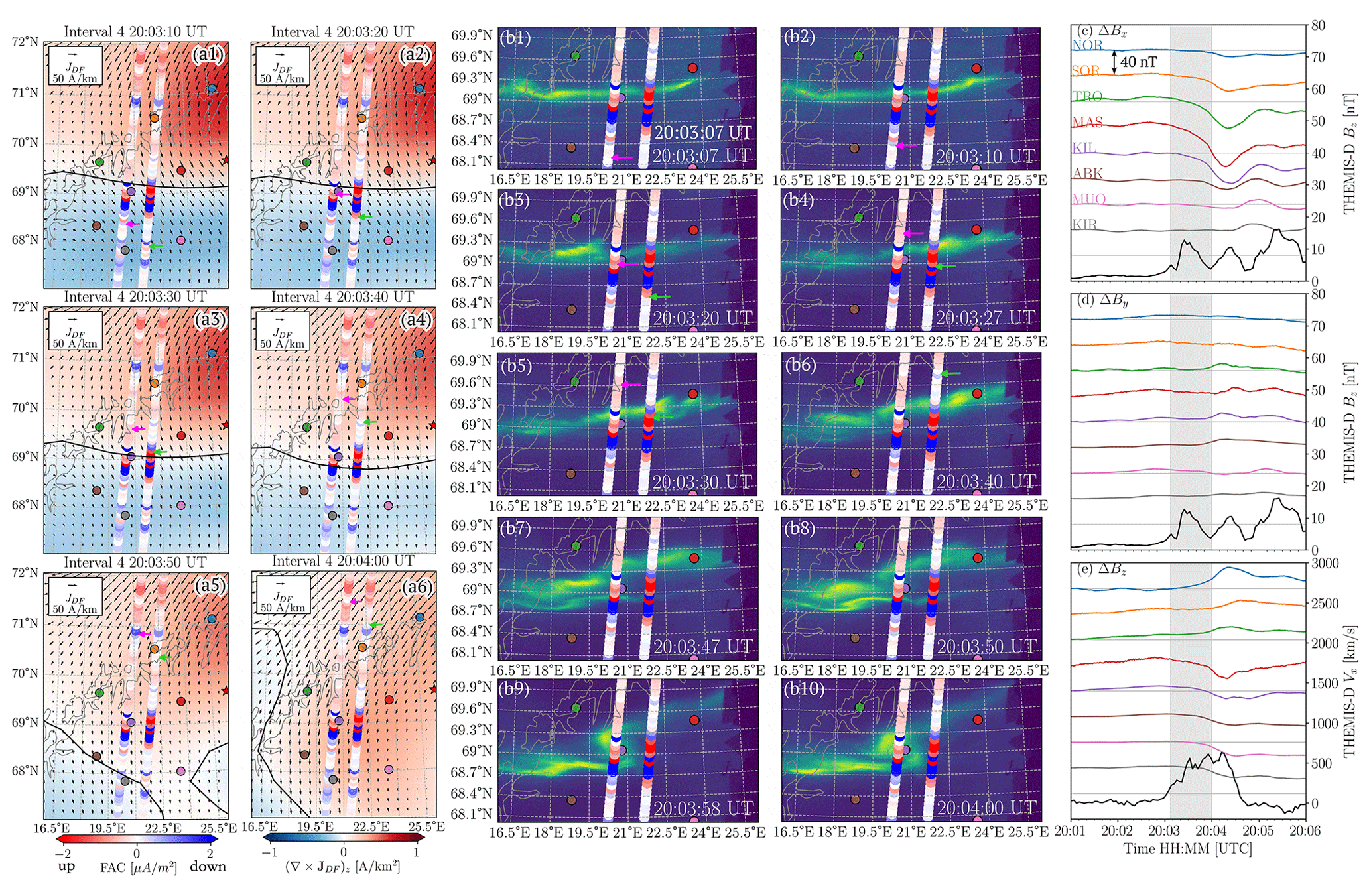
Figure 9Overview of the horizontal and vertical ionospheric currents, auroral activity and ground geomagnetic measurements around the time of the BBF-Swarm conjunction. (a) Snapshots of ionospheric equivalent current map magnitude and direction (arrows) and vorticity (shade) between 20:03:10 and 20:04:00 UT. (b) Auroral activity from KIL ASC projected at 110 km altitude. (c–e) Ground magnetic field observations for eight stations, indicated in panels (a) as colour dots together with THEMIS-D Bz and Vx observations. All traces are evenly spaced with a vertical separation of 40 nT. The gray shaded area marks the interval of the snapshots (20:03:07–20:04:00 UT). Panels (a) and (b) include Swarm A (right trace and green arrow) and Swarm C (left trace and magenta arrow) observations of FAC projected at 110 km.
Between 20:03:07 and 20:03:10 UT, JDF in panel (a1) shows a weak southeastward current, and an auroral arc in panels (b1)–(b2) along the boundary separating the two vortices of opposite vorticity. Around this time, THEMIS-D observations show a slow increase of Bz at 20:02:34 UT, panels (c) and (d), with the sharpest rise occurring between 20:03:08 and 20:03:24 UT, from 5.1 to 12.7 nT, consistent with the arrival of a BBF and the associated dipolarization signature in the near-Earth plasma sheet.
Around 20:03:16 UT Swarm C observes a downward FAC (left trace, blue dots), followed by an upward FAC at 20:03:20 UT (red dots and magenta arrow in panel a2). The auroral arc is latitudinally aligned with this region, panel (b3). 7 to 10 s later, Swarm A (right trace, green arrow) reaches the same location and detects a large downward FAC followed by an upward FAC. The upward FAC is located directly at the position of the auroral arc (b4–b5). The upward–downward FAC pair with µA m−2 extends for about 5 s in the Swarm C data and about 9 s in the Swarm A data, corresponding to approximately 35–50 km along the spacecraft trajectory at Swarm altitude. At the same time, the auroral image shows a clear intensification, with the brightest emission co-located with the upward FAC (green arrow in panel b5), while the BBF footprint lies on the eastern side of the structure. Throughout this 10 s interval, the line of zero vorticity shifts slightly equatorward (panels a3–a4), ΔBx begins to decrease (consistent with a southward displacement of the counterclockwise vortex), and ΔBz increases at the stations north of the arc (NOR, SOR, TRO) while decreasing at the arc latitude (MAS, KIL), with no evident changes at the stations south of the arc (ABK, MUO, KIR).
By 20:03:40 UT, both Swarm A and C have moved beyond the auroral region (b6), and the FAC magnitude is markedly lower. Around 20:03:50 UT, the aurora shows an enhancement on the western side (panels b7–b8), followed by a twisting deformation (b9–b10). At this time, the horizontal currents exhibit a pronounced increase in counterclockwise vorticity and a displacement toward lower latitudes, and the overall current pattern becomes strongly southward, panels (a5)–(a6).
In comparison with THEMIS-D observations, the strongest ground perturbation occurs at 20:04:20 UT, near the end of the interval when THEMIS-D Vx exceeded 150 km s−1 (20:03:05–20:04:32 UT). Around this time, ground Bz also shows large perturbations: the northern stations (NOR, SOR, TRO) record an increase in Bz, while the southern stations (MAS, KIL, ABJ, MUO, KIR) record a decrease. This pattern is consistent with the settled southwestward current (at 20:03:50 UT, panel a5) located between the two station groups, producing increasing Bz north of the current and decreasing Bz to the south.
Figure 10 presents the MS-MVA analysis of Swarm A and Swarm C data between 20:03:00 and 20:03:50 UT. Panel (a) shows the 50 Hz magnetic field perturbation components in NEC. Panel (b) shows the FAC density from low-resolution (1 Hz) data (blue) and from 20 s low-pass filtered data (orange). The spectrograms in panels (c)–(f) show the MS-MVA results performed on sliding time intervals, with their width indicated on the y axis (in seconds of satellite travel duration). Panel (c) shows ratio of the largest and intermediate eigenvalues, while panels (d) and (e) present the derivative of the largest and intermediate eigenvalue with respect to the window scale (the color scale varies logarithmically). Finally, the inclination of the FAC structure, in degrees with respect to the east-west direction, is presented in panel (f). The MS-MVA analysis has been constrained to the plane perpendicular to the local magnetic field direction, which makes the third (smallest) eigenvalue always zero.
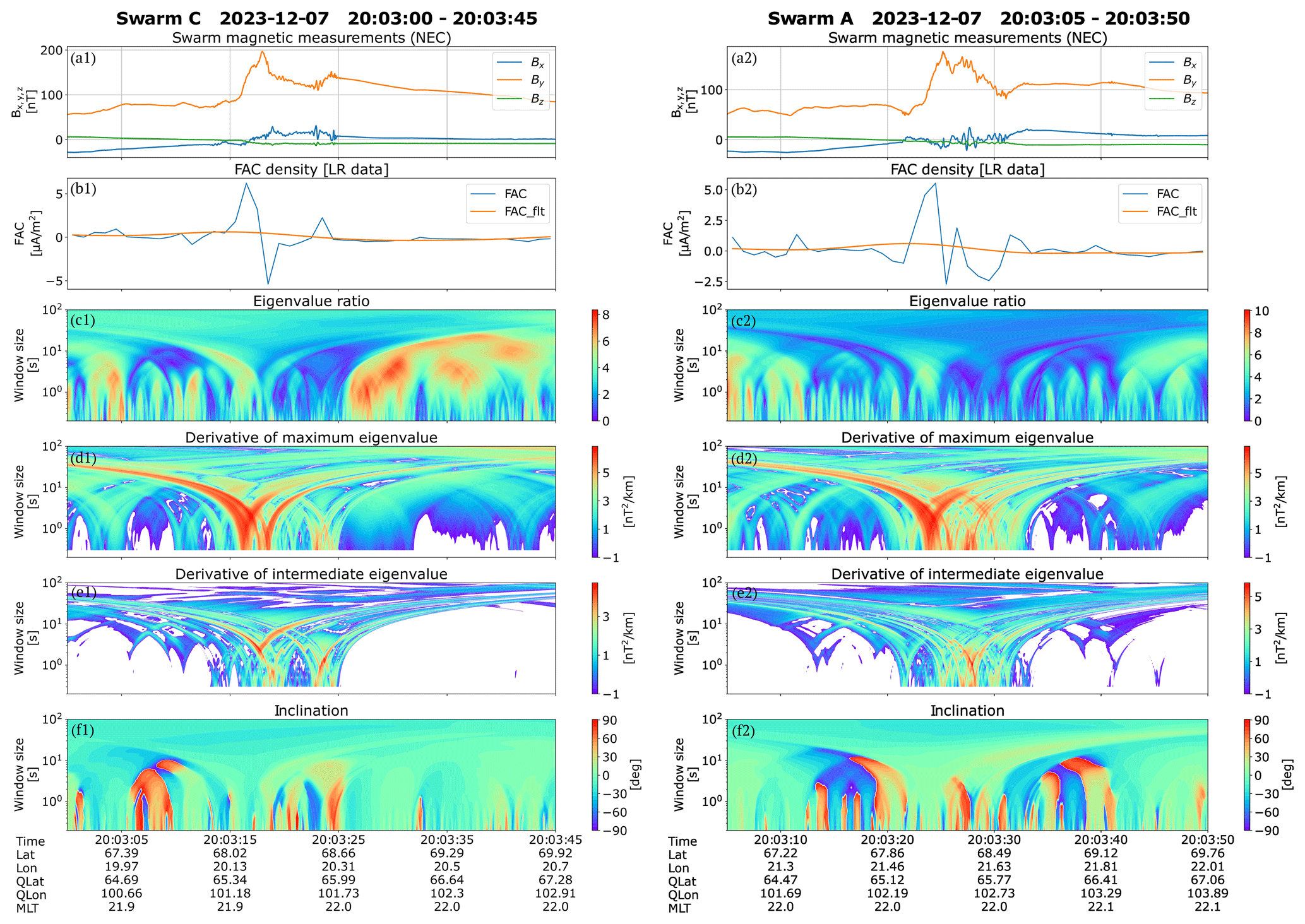
Figure 10Multi-scale minimum variance analysis of Swarm C (left) and Swarm A (right) FAC data on 7 December 2023 20:03:00–20:03:50 UT. (a) Magnetic field perturbation, (b) single spacecraft current density, (c) eigenvalue ratio, (d, e) derivative of the maximum/intermediate eigenvalue with respect to the width of the sliding window, and (f) inclination with respect to east–west direction.
Swarm C is the first spacecraft to enter the region of the largest FAC. The downward and upward current peaks at 6.2 and −5.4 µA m−2 respectively, followed by a secondary downward current of 2.2 µA m−2. Swarm A arrives only 7 s later and observes a similar overall structure: a clear pair of downward (maximum 5.5 µA m−2) and upward (minimum −2.4 µA m−2) FACs, separated by a very localized up/down pair at ∼20:03:25–20:03:28. Considering the optical data, the observation of this narrow FAC pair just by Swarm A, 7 s after Swarm C, appears to be related to both spatial and temporal variations, dominated by the spatial effect. It is tempting to associate this small scale FAC pair with the kinetic structure of the BBF (e.g. Sun et al., 2013), though validating such an association is beyond the scope here.
Figure 10c1 and c2 shows that the strong downward FAC presents larger planarity compared to the upward FAC. In particular, the upward FAC has an eigenvalue ratio close to 1, indicating a highly non-planar structure. This is consistent with the significant derivative of the intermediate eigenvalue in panel (e2) at ∼20:03:28 on Swarm A (the spacecraft closer to the BBF footpoint), which also indicates a finite, non-planar FAC element. The inclination in panel (f), indicates that the downward FAC inclination is east-west oriented (inclination 0°), while the upward FAC is clearly different from east-west (>30°). Both the non-planarity and distinct inclination of the upward FAC structure are consistent with the expected FAC footprint of the BBF current system. According to Birn et al. (2004), earthward moving bubbles are found to be associated with downward FAC on the dawnside and upward FAC on the duskside of the BBF footpoint. The Swarm observations match this geometry. The upward FAC is observed slightly south and west of the BBF footpoint (Fig. 9a), aligned with the expected location of the BBF upward FAC and also with the auroral intensification near Swarm A, visible in the optical frames of 20:03:27 and 20:03:30 UT in panels (b4) and (b5) of Fig. 9. In contrast, the downward FAC observed by Swarm is likely part of a different current system and less likely to be associated with the BBF.
6.1 BBF Intervals
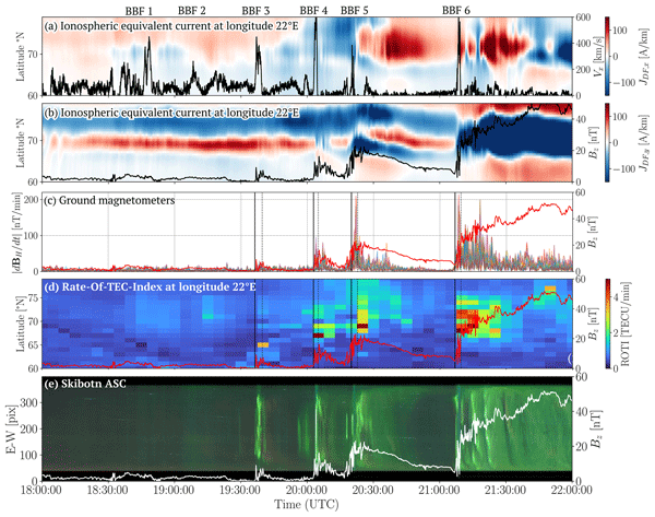
An overview of the horizontal ionospheric current density and auroral activity, together with THEMIS-D observations in the magnetotail between 18:00 and 22:00 UT, is shown in Fig. 11. Panels (a)–(d) show JDF and its vorticity at four different times. Panels (e)–(f) present keograms of the north-south (JDF,x) and east-west (JDF,y) components. The auroral keograms along north-south and east-west cuts are shown in panels (g)–(h), respectively. A summary of the last four BBF intervals is provided in Table 1. From the intervals analyzed in detail in Sect. 4 and summarized in Table 1, the first two intervals (3 and 4) are not classified as substorms in the substorm list provided by SuperMAG identified by the SOPHIE technique (Forsyth et al., 2015), and the auroral images show characteristics consistent with auroral pseudo-breakups. In contrast, the last two intervals (5 and 6) are classified as substorms and exhibit clear auroral breakups. Auroral activity was preexisting before the first pseudo-breakup, with green aurora already observed on the northward horizon of Skibotn at around 18:00 UT.
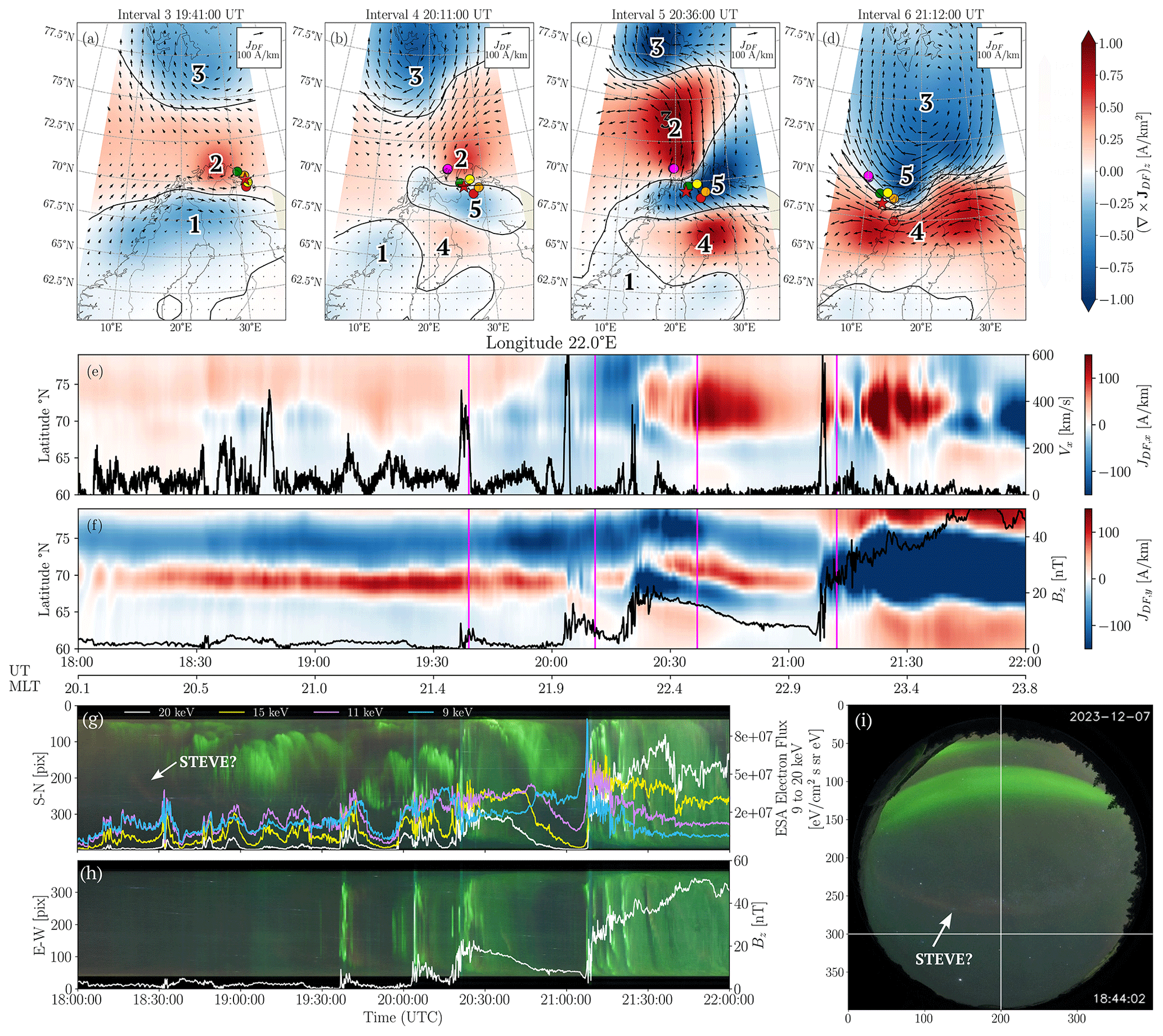
Figure 11Overview of the interval on 7 December 2023 between 18:00 and 22:00 UT, during which six BBFs were detected by THEMIS-D; the last four were accompanied by clear dipolarization signatures. (a–d) Horizontal ionospheric equivalent current density (JDF) magnitude and direction (arrows), its vorticity (∇×JDF)z (shaded), with counterclockwise (red) and clockwise values (blue). The red star marks the BBF footpoint centroid computed from the Tsyganenko models, shown in dots: T89 (red), T96 (orange), T01 (green), and T04 (yellow), TA15n (purple), and TA15b (magenta). (e) Keogram of the north–south current component JDF,x, together with THEMIS-D Vx used for BBF identification. (f) Keogram of the east–west component JDF,y, shown with THEMIS-D Bz to indicate dipolarization. (g) Keogram of the Skibotn auroral images along the central longitude (pix 200), together with THEMIS-D observations of electron flux. (h) Keogram along the latitude cut southward from the Skibotn location (pix 300), together with THEMIS-D Bz. (i) ASC image showing the longitudinal and latitudinal cuts used in panels (g) and (h).
Table 1Summary of four BBF intervals. The BBF time intervals corresponds to the intervals of George et al. (2026) detected by THEMIS-D, except for Interval 5 for which the range is defined to include the BBF detected by THEMIS-A and THEMIS-E. The substorm onset location is taken from the substorm list provided by SuperMAG identified by the SOPHIE technique (Forsyth et al., 2015).

* The BBF footpoint centroid lies outside the field of view of the all-sky camera in Skibotn projected at 110 km.
At approximately 18:16 UT (more clearly by 18:20 UT), a purple auroral arc appears equatorward of the green aurora, which at that time remains low on the northern horizon. This purple arc gradually moves equatorward until about 18:30 UT, where it becomes nearly stationary and merges with additional purple structures that appear as the green aurora brightens and expands equatorward, as shown in Fig. 11g, i. This combined evolution continues until roughly 19:05 UT. After this time, the purple emission becomes mixed with the green aurora, making it difficult to distinguish and track as a separate feature. Based on its color, motion, and equatorward displacement, this early-evening purple arc may correspond to a suprathermal-emission feature such as a STEVE-like structure (MacDonald et al., 2018), although its identification cannot be confirmed unambiguously from the available ASC data. During the interval when the purple aurora is observed, two BBFs were detected by THEMIS-D between 18:30–18:54 UT and 18:58:35–19:19:45 UT, both lacking a clear dipolarization signature and mapping to the East of Finland (Fig. 4a).
The behavior of the ionospheric horizontal currents can only be examined starting with Interval 3, because in Intervals 1 and 2 the BBF footpoint centroid is located east of the area covered by the IEQ current maps. Throughout Interval 3, the horizontal currents retain the characteristic structure of the Harang discontinuity, Fig. 11a, with variations primarily in current magnitude rather than direction. Around the equatorward flank of the eastward electrojet, an auroral arc intensifies at the same time that THEMIS-D detects the BBF and the dipolarization front, Figs. 5b2 and 11g, and an increase in electron flux, Fig. 11h. The auroral evolution shows signatures of a pseudo-breakup, consistent with what is expected during the BBF, although the BBF footpoint centroid lies westward of the field-of-view of the ASC. However, from the THEMIS-D observations, it is not a pseudo-substorm; note that our BBF velocity is much larger than that in Table 2 of Fukui et al. (2020). Despite the BBF speed being larger than that observed during interval 5, the associated dipolarization is weak and returns to pre-dipolarization values after roughly 10 min.
Due to the relatively quiet geomagnetic conditions during the observations of the BBF in this interval, the BBF footpoint does not show much spread among models, and the magnetosphere is expected to remain without strong changes. Thus, this interval is a good event to place the BBF footpoint in the general context. Both Interval 2 and Interval 3 show very similar characteristics, with a Harang discontinuity structure, and the BBF mapping in the region of strong counterclockwise vorticity (upward FAC) and poleward turning of the horizontal ionospheric currents.
Although Interval 4 is not identified as a substorm by SOPHIE, a decrease in Bx is observed at magnetometer stations located at similar latitudes as the BBF footpoint (TRO, KIL, and MAS). The largest drop, recorded at MAS, is of approximately 68 nT in 1.5 min, Fig. 9c. The auroral images in Fig. 6b show an intensification of the pre-existing arc at onset and a subsequent breakup into two branches, but without the clear poleward expansion or equatorward motion characteristic of a full substorm (see Supplement Movie for the full sequence), indicating that this interval corresponds to a pseudo-breakup. The horizontal equivalent current map in Fig. 11b displays a pattern similar to that of Interval 5: a westward current emerges at the same time the dipolarization is observed (between vortex 4 and 5), although with much weaker magnitude, and then drifts equatorward. This is also observed in Fig. 11f, where positive JDF,y appears around 65° N. Five vortices are identified, Fig. 11b, with the same arrangement as in Interval 5, but with vortex 2 located farther east than during Interval 5. This shift results in a predominantly southward current instead of a northward one. Before the dipolarization Bz fully returns to its pre-dipolarization level, the BBF associated with Interval 5 arrives, interrupting the evolution of the current system.
The FACs derived from the single-spacecraft measurements of Swarm A and Swarm C reveal a clear upward FAC at the location of the auroral arc and a downward FAC immediately to the south, Fig. 9b4. Both regions extend over a north–south distance of approximately 35–50 km, Fig. 9b3–b4. However, when using the dual-satellite method, which resolves only structures larger than 150 km, this localized pair of upward and downward currents is smoothed out, leaving only a broader region of downward FAC. This large-scale downward current coincides with the region of clockwise vorticity in the horizontal ionospheric equivalent currents derived from IMAGE magnetometers at 10 s resolution. Together, these observations demonstrate that the BBF-related FAC system contains significant small-scale structure that is captured only by the single-satellite approach, and that the characteristic scales of these currents are comparable to those expected for narrow auroral arcs.
This result is qualitatively consistent with the findings of Forsyth et al. (2014), who showed that the FAC structures within the SCW tend to be aligned predominantly north–south rather than east–west. Such north–south-oriented FAC elements are typically associated with the appearance of north–south auroral streamers during the expansion-phase bulge (Partamies et al., 2006). Our individual BBF event, even if rather intense (high speed), can be hardly compared with the expansion phase bulge. However, the FAC features derived by the MS-MVA (Sect. 5) are rather consistent with a north-south streamer. A possible explanation for the absence of a clear optical signature could be a weak energy flux, directly related to faint luminosity, perhaps sub-visual, unlike the strong energy flux and accordingly bright streamers of the expansion bulge.
Interval 5 corresponds to a substorm that occurred approximately 9 min after the previous event and 50 min before the onset identified in Interval 6. The SuperMAG onset location lies at roughly the same latitude as the BBF ionospheric footpoint but displaced about 8° westward, near the west coast of Norway. Ground magnetometers show a clear decrease in Bx of about −150 nT, followed by a pronounced decrease in By while Bx recovers, which results in a strong northward ionospheric current (Fig. A1). The auroral images exhibit the typical evolution of an auroral substorm, with the brightening and subsequent break-up of the pre-existing arc. After the time shown in Fig. 7a4, vortices 2 and 5 intensify, producing the strong northward current; vortex 4 begins to move westward and elongates in the east–west direction; and vortex 1 weakens. The evolution of the horizontal currents is interrupted by the onset of the subsequent substorm (Interval 6), but these currents had already begun to diminish as the dipolarization signature returned to its pre-dipolarization level.
Finally, interval 6 is the interval that most clearly corresponds to the classical substorm-onset sequence (Akasofu, 1964; McPherron et al., 1973). Figures 8 and 11f, g, h show that during this interval a WEJ is formed, and the auroral signatures follow the expected onset progression: an auroral arc intensifies at 21:06:02 UT, bifurcates and begins a poleward expansion by 21:07:32 UT, reaches its maximum poleward extent at 21:09:01 UT, and subsequently undergoes breakup followed by equatorward and eastward motion. Simultaneously, a BBF is observed together with a clear dipolarization in the magnetotail, and an increase of the electron flux with energies between 9–20 keV, Fig. 11g. This combination of BBF arrival, dipolarization, electrojet intensification, and auroral evolution is fully consistent with the onset and early expansion phase of a substorm.
An interesting feature of Interval 6 is that the substorm onset identified by SOPHIE is located approximately 20° west of the BBF ionospheric footpoint. The ground magnetic measurements show a clear decrease in Bx, reaching a minimum of about −500 nT, together with an increase in By, resulting in a northwestward electrojet (Fig. A1). After this initial development, while the WEJ continues to intensify, it also propagates equatorward and westward. This motion produces a systematic change in the north–south component of the horizontal ionospheric current: the current is directed northward on the western flank of the electrojet and southward on its eastern flank. This evolution reflects the lateral displacement and strengthening of the WEJ during the early expansion phase of the substorm.
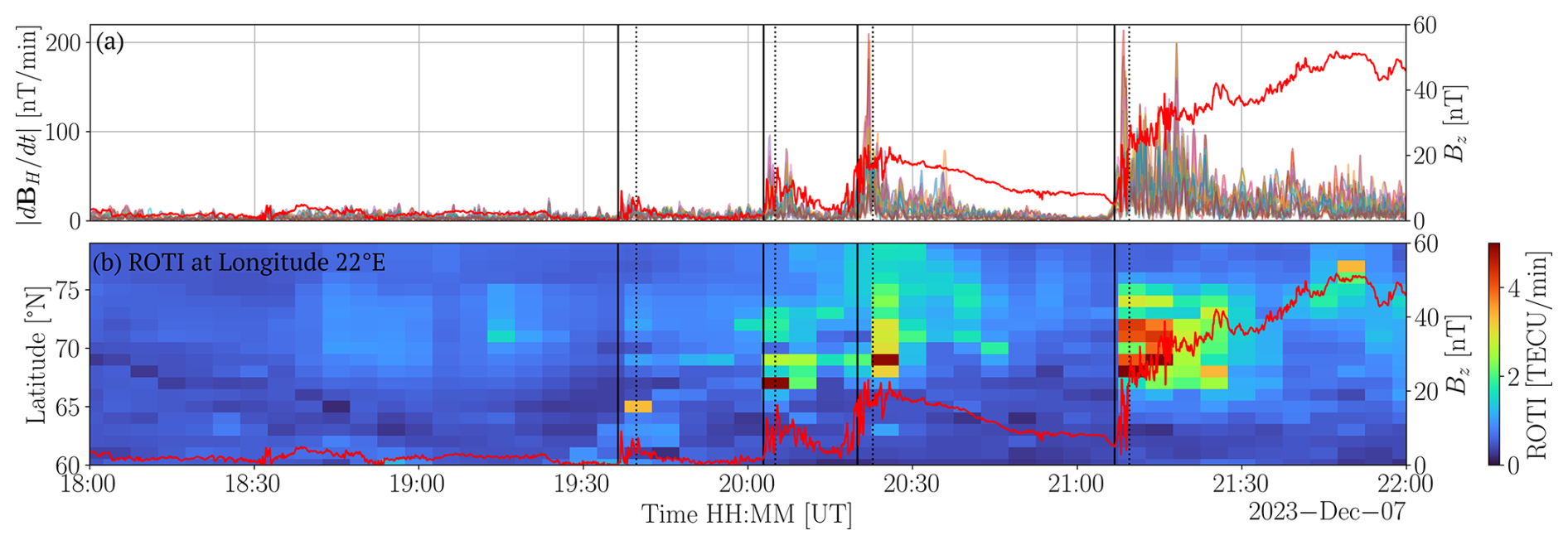
Figure 12Space weather response to the dipolarization. (a) Ground magnetic field perturbation for each station shown in Fig. 4b, together with the Bz observations by THEMIS-D. (b) Keogram of the ROTI, together with the Bz observations by THEMIS-D. The vertical lines indicate the beginning (solid) and end (dashed) times of the four BBFs intervals listed in Table 1.
The auroral signatures observed during the last four BBFs consisted of an intensification of a pre-existing auroral arc (Fig. 11h), together with enhancements in 9–20 keV electron fluxes that mapped directly to the arc (Fig. 11g). None of the BBFs in this event produced auroral streamers. This is consistent with previous multipoint conjugate studies between THEMIS and all-sky cameras (e.g., Keiling et al., 2009; Panov et al., 2013, 2016), which show that BBF-driven auroral feedback commonly appears as brightening of pre-existing arcs, auroral bulge intensification, poleward expansion, or the development of spiral or fork-like structures rather than streamer-type signatures. This complex auroral behavior is not surprising, as the THEMIS spacecraft were located in the BBF flow-braking region (Shiokawa et al., 1997; Baumjohann et al., 1999), where high-speed earthward flows decelerate and generate plasma-flow vortices. Simultaneously, these previous studies reported conjugate ionospheric flow vortices with opposite rotational sense on either side of a westward electrojet, a configuration similar to that observed during Interval 6.
6.2 Space weather impacts
We briefly assess the space weather impacts associated with the BBFs/dipolarization. Using the magnetometer stations shown in Fig. 4b, we computed the horizontal magnetic field perturbation, with each station plotted as a separate trace in Fig. 12a. The enhancements occur simultaneously with the last four dipolarization events, with peak amplitudes increasing with the progression of the events. The largest perturbation reached 213 nT min−1 at the TRO station during Interval 6, while Interval 5 produced a comparable peak of 209 and 201 nT min−1 at the NOR and SOR stations, respectively. For context, Rosenqvist et al. (2025) reported peaks associated with power-grid disturbances, and 10 of the 23 events in their list exhibited maxima below 213 nT min−1. This suggests that BBFs accompanied by strong dipolarization fronts may be capable of producing ground magnetic perturbations of similar magnitude. However, the geophysical conditions differ: the highest-latitude station in Rosenqvist et al. (2025) was located at 66.5° N, whereas TRO lies at 69.7° N, and the Hp30 index during our event (3.3) was lower than the Hp30≥4 in their study. Electron density irregularities show a similar temporal correspondence. As illustrated in Fig. 12b, the ROTI intensifies in step with each dipolarization, with the strongest enhancements occurring during the last two BBF/dipolarization intervals. These ROTI peaks appear near 67–69° N, consistent with the latitudinal location of the BBF ionospheric footprints centroid listed in Table 1.
Taken together, these observations demonstrate that BBFs and their associated dipolarization fronts can generate localized but intense space weather signatures in both the magnetic field and ionospheric plasma. Although the magnitudes observed here fall below those typically linked to power-grid disturbances, the temporal and latitudinal coherence of the magnetic and ionospheric responses highlights the capacity of BBF-driven processes to produce sharp, small-scale perturbations during moderately disturbed conditions.
In this work, we present a fortuitous constellation of events and observations from both the near-Earth magnetotail and the high-latitude ionosphere on 7 December 2023 between 18:00 and 22:00 UT, which increases our understanding of the coupling between these regions:
-
The BBF maps to a region where a counterclockwise vorticity structure in the horizontal ionospheric equivalent current is established during the flow arrival.
-
The auroral arc brightens at the same time that the magnetotail exhibits both the earthward bulk flow and the associated dipolarization.
-
At the time of the BBF and the associated dipolarization, an increase in the 9–20 keV electron flux is also observed. These electrons, after traveling along field-lines to the ionosphere, are capable of producing the auroral brightening. Additional near-Earth acceleration at ∼1RE seems not needed to explain this event.
-
Large scale upward/downward FACs (larger than 150 km) derived from the Swarm spacecraft dual-satellite method correspond to the regions of counterclockwise/clockwise vorticity of the horizontal ionospheric equivalent currents.
-
Localized intense FAC related to aurora arcs and BBF events have a scale of around 35–50 km that are only detected by the Swarm single spacecraft FAC. The dual spacecraft method lack the spatial resolution to reveal significant additional information.
-
A localized, strong upward FAC is detected southwest of the BBF footpoint, characterized by high non-planarity and a clear inclination relative to the east–west direction.
-
None of the BBFs within this event seems to be related to auroral streamers.
-
BBFs with stronger dipolarization show larger space weather impact on ground magnetic disturbances and electron density irregularities, than BBFs with similar velocity magnitude but weaker or no dipolarization.
According to the SCW model (McPherron et al., 1973), dipolarization is an expected signature of the reconfiguration of the near-Earth magnetotail during substorm onset. This reconfiguration of the magnetic field/currents is associated with increased downward Poynting flux in the topside ionosphere as seen in many studies, and with dissipation/Joule heating. Also, mainly in the lower thermosphere, a closure current jc transfers momentum via the Lorentz force jc×B. This momentum is not supplied by magnetic field reconfigurations but rather by plasma deceleration and acceleration. The model of substorm energy released from a stretched tail field needs some adjustment: required is a conversion of this energy first to mechanical flow, providing both momentum and energy which then are transferred to the high-latitude ionosphere-thermosphere via FACs/magnetic stresses. These considerations certainly are not new, but our analysis demonstrates a clear association of both BBF and dipolarization mapped in space and time with the observed auroral (pseudo)breakups, FACs and geomagnetic signatures.
While previous studies combining THEMIS with all-sky images and SECS analysis have reported ionospheric feedback to magnetotail BBFs during weak substorm intervals (e.g., Keiling et al., 2009; Panov et al., 2013, 2016), this study provides the first direct, multi-instrument observation of how a sequence of recurrent BBFs produces a coherent and time-aligned chain of magnetotail–ionosphere coupling signatures: localized counterclockwise vorticity in the horizontal ionospheric currents and discrete auroral arc intensification around the BBF footpoint, and in some intervals, enhancements in 9–20 keV electron fluxes in the magnetotail that map directly to the auroral arcs. From a space weather perspective, our results reinforce that BBFs with strong dipolarization can generate localized FACs that modify the large scale current system and drive density irregularities, even in the absence of a full substorm. Such BBF driven disturbances may therefore contribute to isolated geomagnetic perturbations capable of driving localized GICs and ionospheric irregularities that degrade GNSS performance.
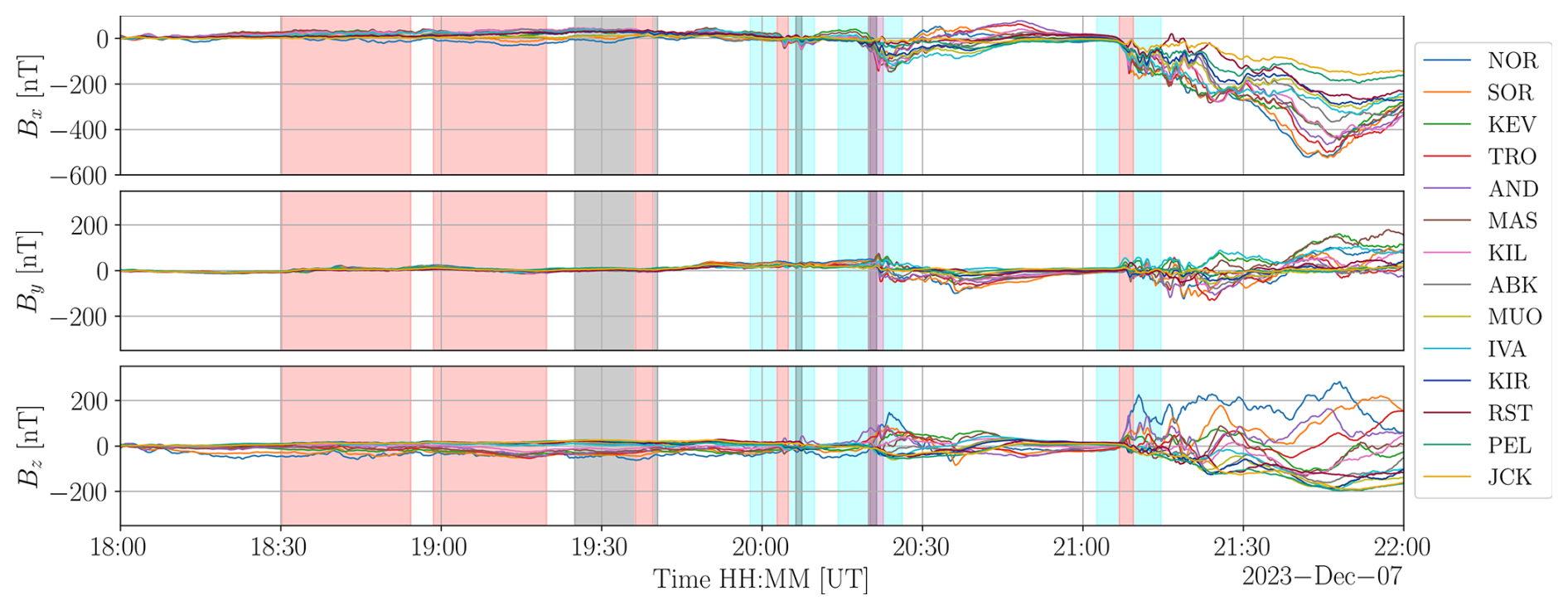
IMAGE data is available at the website https://space.fmi.fi/image/ (last access: 25 March 2026). A code for the SECS analysis is available in Vanhamäki and Juusola (2020). The footpoints for each BBF events were computed using the Geopack tracing routine for the Tsyganenko models T89, T96, T01, and T04, available through the Geopack Python library (https://github.com/tsssss/geopack) (last access: 22 August 2025), and TA15b, TA15n, available through the IDL Geopack DLM (https://korthhaus.com/idl-software/idl-geopack-dlm/) (last access: 22 August 2025). THEMIS and Swarm positions were mapped to 110 km using the AACGM python package https://github.com/aburrell/aacgmv2 (last access: 15 September 2026) (Shepherd, 2014). The THEMIS data were accessed using the open-source Python Space Physics Environment Data Analysis Software (pySPEDAS) by Grimes et al. (2022), which can be found at https://github.com/spedas/pyspedas (last access: 21 February 2026). Solar wind data from ACE, and geomagnetic indices (AL, AU and Sym-h) are available at the Coordinated Data Analysis Web of NASA's Goddard Flight Center https://cdaweb.gsfc.nasa.gov (last access: 20 April 2026). Hp30 index is available from the GFZ website https://www.gfz-potsdam.de/en/hpo-index (last access: 20 April 2026). We use the Python package, viresclient (Smith et al., 2025), to access Swarm Level 2 data from ESA’s VirES for Swarm service https://vires.services/ (last access: 23 April 2026) and the dual-sat FAC_LLS data, available on the Swarm dissemination server (last access: 11 May 2026). The images from the all-sky color camera at Skibotn can be downloaded from http://darndeb08.cei.uec.ac.jp/~nanjo/public/skibotn_imgs/2023_season/20231207/ (last access: 31 March 2026). KIL ASC images can be downloaded from https://doi.org/10.5281/zenodo.21495156 (Hoppe, 2026).
The video in the video supplement (https://doi.org/10.5446/73085) (Lanabere, 2026) illustrates the time evolution of the horizontal ionospheric equivalent current density and its vorticity, the auroral activity from Skibotn all-sky camera, and THEMIS-D observations of Vx, Bz, and electron flux. The animations consist of frames similar to those shown in panels (a) and (b) from Figs. 5–8.
V. L. conceptualized the study, prepared the manuscript, produced the figures, and performed the analysis. S. B. provided guidance for the study. A. B. provided the MS-MVA figures and FAC data from Swarm. H. G. provided the BBFs dataset and contributed to the writing. S. N. and Y. J. provided the data and projection matrix of the Skibotn ASC. T. H. provided the data from the Kilpisjärvi ASC. L. J. contributed to the physical analysis and provided code projection of KIL ASC. All read and provided feedback on the manuscript.
The contact author has declared that none of the authors has any competing interests.
Publisher's note: Copernicus Publications remains neutral with regard to jurisdictional claims made in the text, published maps, institutional affiliations, or any other geographical representation in this paper. The authors bear the ultimate responsibility for providing appropriate place names. Views expressed in the text are those of the authors and do not necessarily reflect the views of the publisher.
A. P. D. received financial support from the Swedish National Space Agency (grant no. 2020-00111). A.B. and O.M. acknowledge support from the project MAGICS, ESA PRODEX (grant no. 4000127660), as well as the efficient and handy implementation of the MS-MVA technique by Prof. Joachim Vogt from Constructor University Bremen. S. W. and J. A. C. are supported by Royal Society (grant no. DHF/R1/211068). L. J. acknowledges funding from the Research Council of Finland (grant no. 374099-SpaceResilience). A. A. acknowledges funding from the Research Council of Finland (grant nos. 374100-SpaceResilience and 348782 INTERSECT). H. V. acknowledges funding from the Research Council of Finland (grant no. 354521 AuroralJoule). Y. J. and D. K. acknowledge funding from the European Research Council (ERC) under the European Union's Horizon 2020 research and innovation program (ERC Consolidator grant no. 866357, POLAR-4DSpace). V. L., A. P. D., S. B., O. M., L. R., L. J., J. A. C., and S. W. would like to acknowledge the discussions with members of the ISSI/ISSI-BJ International Team project “Understanding ground magnetic disturbances due to field-aligned currents driven by magnetotail activity” (ISSI Team project #24-614; ISSI-BJ Team project #63) supported by the International Space Science Institute (ISSI) in Bern and Beijing. We thank Dr. Magnar Gullikstad Johnsen from Tromsø Geophysical Observatory, UiT – the Arctic University of Norway, for providing the 1 s magnetometer data from NOR, SOR, and TRO. We thank Dr. Masatoshi Yamauchi (IRF) for providing 1 s data from KIR data. We thank Dr. Stefan Eriksson from the Laboratory for Atmospheric and Space Physics, Boulder, US, for his comments and suggestions on the manuscript. We thank the institutes who maintain the IMAGE Magnetometer Array: Tromsø Geophysical Observatory of UiT the Arctic University of Norway (Norway), Finnish Meteorological Institute (Finland), Institute of Geophysics Polish Academy of Sciences (Poland), GFZ German Research Centre for Geosciences (Germany), Geological Survey of Sweden (Sweden), Swedish Institute of Space Physics (Sweden), Sodankylä Geophysical Observatory of the University of Oulu (Finland), DTU Technical University of Denmark (Denmark), and Science Institute of the University of Iceland (Iceland). The provisioning of data from AAL, GOT, HAS, NRA, VXJ, FKP, SIN, BOR, SCO and KUL is supported by the ESA (grant nos. 4000128139/19/D/CT and 4000138064/22/D/KS). Copilot Version 25.1 for grammar and language refinement during the preparation of this manuscript.
This research has been supported by the European Space Agency 4D ionosphere initiative (grant nos. 4000143412/23/I-EB (FBURST) and 4000143413/23/I-EB (Swarm-VIP-Dynamic)) and the Vetenskapsrådet (grant no. 2021-06259).
The publication of this article was funded by the Swedish Research Council, Forte, Formas, and Vinnova.
This paper was edited by Elena Kronberg and reviewed by two anonymous referees.
Akasofu, S.-I.: The development of the auroral substorm, Planet. Space Sci., 12, 273–282, https://doi.org/10.1016/0032-0633(64)90151-5, 1964. a, b
Amm, O.: Ionospheric Elementary Current Systems in Spherical Coordinates and Their Application., J. Geomagn. Geoelectr., 49, 947–955, https://doi.org/10.5636/jgg.49.947, 1997. a
Amm, O. and Viljanen, A.: Ionospheric disturbance magnetic field continuation from the ground to the ionosphere using spherical elementary current systems, Earth Planets Space, 51, 431, https://doi.org/10.1186/BF03352247, 1999. a
Angelopoulos, V.: The THEMIS Mission, Space Sci. Rev., 141, 5–34, https://doi.org/10.1007/s11214-008-9336-1, 2008. a
Baker, D. N., Pulkkinen, T. I., Hesse, M., and McPherron, R. L.: A quantitative assessment of energy storage and release in the Earth's magnetotail, J. Geophys. Res., 102, 7159–7168, https://doi.org/10.1029/96JA03961, 1997. a
Baker, K. B. and Wing, S.: A new magnetic coordinate system for conjugate studies at high latitudes, J. Geophys. Res., 94, 9139–9143, https://doi.org/10.1029/JA094iA07p09139, 1989. a
Baumjohann, W., Paschmann, G., and Lühr, H.: Characteristics of high-speed ion flows in the plasma sheet, J. Geophys. Res., 95, 3801–3809, https://doi.org/10.1029/JA095iA04p03801, 1990. a
Baumjohann, W., Hesse, M., Kokubun, S., Mukai, T., Nagai, T., and Petrukovich, A. A.: Substorm dipolarization and recovery, J. Geophys. Res., 104, 24995–25000, https://doi.org/10.1029/1999JA900282, 1999. a, b
Birn, J. and Hesse, M.: The substorm current wedge in MHD simulations, J. Geophys. Res., 118, 3364–3376, https://doi.org/10.1002/jgra.50187, 2013. a
Birn, J. and Hesse, M.: The substorm current wedge: Further insights from MHD simulations, J. Geophys. Res., 119, 3503–3513, https://doi.org/10.1002/2014JA019863, 2014. a
Birn, J., Raeder, J., Wang, Y. L., Wolf, R. A., and Hesse, M.: On the propagation of bubbles in the geomagnetic tail, Ann. Geophys., 22, 1773–1786, https://doi.org/10.5194/angeo-22-1773-2004, 2004. a
Blagau, A. and Vogt, J.: Multipoint Field-Aligned Current Estimates With Swarm, J. Geophys. Res., 124, 6869–6895, https://doi.org/10.1029/2018JA026439, 2019. a
Blagau, A. and Vogt, J.: SwarmFACE: A Python package for field-aligned currents exploration with Swarm, Frontiers in Astronomy and Space Sciences, 9, https://doi.org/10.3389/fspas.2022.1077845, 2023. a
Borodkova, N. L., Yahnin, A. G., Liou, K., Sauvaud, J.-A., Fedorov, A. O., Lutsenko, V. N., Nozdrachev, M. N., and Lyubchich, A. A.: Plasma sheet fast flows and auroral dynamics during substorm: a case study, Ann. Geophys., 20, 341–347, https://doi.org/10.5194/angeo-20-341-2002, 2002. a
Bunescu, C.: The Structure of Field-Aligned Current Systems as Inferred From the Multiscale Minimum Variance Analysis, Earth and Space Science, 11, e2024EA003708, https://doi.org/10.1029/2024EA003708, 2024. a
Bunescu, C., Marghitu, O., Constantinescu, D., Narita, Y., Vogt, J., and Blăgău, A.: Multiscale field-aligned current analyzer, J. Geophys. Res., 120, 9563–9577, https://doi.org/10.1002/2015JA021670, 2015. a
Bunescu, C., Vogt, J., Marghitu, O., and Blagau, A.: Multiscale estimation of the field-aligned current density, Ann. Geophys., 37, 347–373, https://doi.org/10.5194/angeo-37-347-2019, 2019. a
Burt, J. and Smith, B.: Deep space climate observatory: The DSCOVR mission, in: 2012 IEEE Aerospace Conference, IEEE, 1–13, https://doi.org/10.1109/AERO.2012.6187025, 2012. a
Buzulukova, N. and Tsurutani, B.: Space Weather: From solar origins to risks and hazards evolving in time, Frontiers in Astronomy and Space Sciences, 9, https://doi.org/10.3389/fspas.2022.1017103, 2022. a
Chisham, G., Lester, M., Milan, S. E., Freeman, M. P., Bristow, W. A., Grocott, A., McWilliams, K. A., Ruohoniemi, J. M., Yeoman, T. K., Dyson, P. L., Greenwald, R. A., Kikuchi, T., Pinnock, M., Rash, J. P. S., Sato, N., Sofko, G. J., Villain, J.-P., and Walker, A. D. M.: A decade of the Super Dual Auroral Radar Network (SuperDARN): scientific achievements, new techniques and future directions, Surv. Geophys., 28, 33–109, https://doi.org/10.1007/s10712-007-9017-8, 2007. a
Crooker, N. U., Kahler, S. W., Larson, D. E., and Lin, R. P.: Large-scale magnetic field inversions at sector boundaries, J. Geophys. Res., 109, https://doi.org/10.1029/2003JA010278, 2004. a
Davis, T. N. and Sugiura, M.: Auroral electrojet activity index AE and its universal time variations, J. Geophys. Res. (1896–1977), 71, 785–801, https://doi.org/10.1029/JZ071i003p00785, 1966. a
Engebretson, M. J., Gaffaney, S. A., Ochoa, J. A., Runov, A., Weygand, J. M., Nishimura, Y., Hartinger, M. D., Pilipenko, V. A., Moldwin, M. B., Connors, M. G., Mann, I. R., Xu, Z., and Rodriguez, J. V.: Signatures of Dipolarizing Flux Bundles in the Nightside Auroral Zone, J. Geophys. Res., 129, e2023JA032266, https://doi.org/10.1029/2023JA032266, 2024. a
Farris, M. H. and Russell, C. T.: Determining the standoff distance of the bow shock: Mach number dependence and use of models, J. Geophys. Res., 99, 17681–17690, https://doi.org/10.1029/94JA01020, 1994. a
Feng, X., Yang, J., Bortnik, J., Wang, C.-P., and Liu, J.: Predicting characteristics of bursty bulk flows in Earth’s plasma sheet using machine learning techniques, Frontiers in Astronomy and Space Sciences, 12, https://doi.org/10.3389/fspas.2025.1582607, 2025. a, b
Forsyth, C., Fazakerley, A. N., Rae, I. J., Watt, C. E. J., Murphy, K., Wild, J. A., Karlsson, T., Mutel, R., Owen, C. J., Ergun, R., Masson, A., Berthomier, M., Donovan, E., Frey, H. U., Matzka, J., Stolle, C., and Zhang, Y.: In situ spatiotemporal measurements of the detailed azimuthal substructure of the substorm current wedge, J. Geophys. Res., 119, 927–946, https://doi.org/10.1002/2013JA019302, 2014. a
Forsyth, C., Rae, I. J., Coxon, J. C., Freeman, M. P., Jackman, C. M., Gjerloev, J., and Fazakerley, A. N.: A new technique for determining Substorm Onsets and Phases from Indices of the Electrojet (SOPHIE), J. Geophys. Res., 120, 10592–10606, https://doi.org/10.1002/2015JA021343, 2015. a, b
Friis-Christensen, E., Lühr, H., Knudsen, D., and Haagmans, R.: Swarm – An Earth Observation Mission investigating Geospace, Adv. Space Res., 41, 210–216, https://doi.org/10.1016/j.asr.2006.10.008, 2008. a
Fukui, K., Miyashita, Y., Machida, S., Miyoshi, Y., Ieda, A., Nishimura, Y., and Angelopoulos, V.: A Statistical Study of Near-Earth Magnetotail Evolution During Pseudosubstorms and Substorms With THEMIS Data, J. Geophys. Res., 125, e2019JA026642, https://doi.org/10.1029/2019JA026642, 2020. a, b
George, H., Ergun, R., Rogers, A., Genestreti, K., and Gabrielse, C.: Cross-tail extent of magnetotail reconnection from bursty bulk flow distribution, ESS Open Archive, 0914, https://doi.org/10.22541/essoar.15008751/v1, 2026. a, b, c, d
Grimes, E. W., Harter, B., Hatzigeorgiu, N., Drozdov, A., Lewis, J. W., Angelopoulos, V., Cao, X., Chu, X., Hori, T., Matsuda, S., Jun, C.-W., Nakamura, S., Kitahara, M., Segawa, T., Miyoshi, Y., and Le Contel, O.: The Space Physics Environment Data Analysis System in Python, Frontiers in Astronomy and Space Sciences, 9, https://doi.org/10.3389/fspas.2022.1020815, 2022. a, b
Harten, R. and Clark, K.: The Design Features of the GGS Wind and Polar Spacecraft, Space Sci. Rev., 71, 23–40, https://doi.org/10.1007/BF00751324, 1995. a
Hoppe, T.: All-sky camera images from Kilpisjärvi (KIL) on December 7th, 2023 20:03–20:04 UT, Zenodo [figure], https://doi.org/10.5281/zenodo.21495156, 2026. a
Huang, C.-S., Foster, J. C., Goncharenko, L. P., Reeves, G. D., Chau, J. L., Yumoto, K., and Kitamura, K.: Variations of low-latitude geomagnetic fields and Dst index caused by magnetospheric substorms, J. Geophys. Res., 109, https://doi.org/10.1029/2003JA010334, 2004. a
Iyemori, T., Araki, T., Kamei, T., and Takeda, M.: Mid-latitude geomagnetic indices ASY and SYM (provisional) No. 1 1989, Data Analysis Center for Geomagnetism and Space Magnetism, Kyoto University, Kyoto, https://wdc.kugi.kyoto-u.ac.jp/wdc/pdf/indexplot/01%20Mid-latitude%20Geomagnetic%20Indices%20ASY%20and%20SYM%20(Provisional)(1989-1990).pdf (last access: 20 April 2026), 1992. a
Juusola, L., Nakamura, R., Amm, O., and Kauristie, K.: Conjugate ionospheric equivalent currents during bursty bulk flows, J. Geophys. Res., 114, https://doi.org/10.1029/2008JA013908, 2009. a
Juusola, L., Kauristie, K., Vanhamäki, H., Aikio, A., and van de Kamp, M.: Comparison of auroral ionospheric and field-aligned currents derived from Swarm and ground magnetic field measurements, J. Geophys. Res., 121, 9256–9283, https://doi.org/10.1002/2016JA022961, 2016. a
Juusola, L., Vanhamäki, H., Viljanen, A., and Smirnov, M.: Induced currents due to 3D ground conductivity play a major role in the interpretation of geomagnetic variations, Ann. Geophys., 38, 983–998, https://doi.org/10.5194/angeo-38-983-2020, 2020. a
Juusola, L., Viljanen, A., Partamies, N., Vanhamäki, H., Kellinsalmi, M., and Walker, S.: Three principal components describe the spatiotemporal development of mesoscale ionospheric equivalent currents around substorm onsets, Ann. Geophys., 41, 483–510, https://doi.org/10.5194/angeo-41-483-2023, 2023. a
Keiling, A., Angelopoulos, V., Runov, A., Weygand, J., Apatenkov, S. V., Mende, S., McFadden, J., Larson, D., Amm, O., Glassmeier, K.-H., and Auster, H. U.: Substorm current wedge driven by plasma flow vortices: THEMIS observations, J. Geophys. Res., 114, https://doi.org/10.1029/2009JA014114, 2009. a, b
Kepko, L., McPherron, R. L., Amm, O., Apatenkov, S., Baumjohann, W., Birn, J., Lester, M., Nakamura, R., Pulkkinen, T. I., and Sergeev, V.: Substorm Current Wedge Revisited, Space Sci. Rev., 190, 1–46, https://doi.org/10.1007/s11214-014-0124-9, 2015. a
Koskinen, H. E. J. and Pulkkinen, T. I.: Midnight velocity shear zone and the concept of Harang discontinuity, J. Geophys. Res., 100, 9539–9547, https://doi.org/10.1029/95JA00228, 1995. a
Lanabere, V.: Ionospheric currents and auroral signatures during successive earthward bursty bulk flows and dipolarization: a 7 December 2023 case study, TIB [video], https://doi.org/10.5446/73085, 2026. a
Lanabere, V., Dimmock, A. P., Richard, L., Buchert, S., Khotyaintsev, Y. V., and Marghitu, O.: Variability in footpoint mapping of bursty bulk flows using Tsyganenko models: impact on Swarm conjunctions, J. Space Weather Spac., 15, 41, https://doi.org/10.1051/swsc/2025035, 2025. a
Lepping, R. P., Acũna, M. H., Burlaga, L. F., Farrell, W. M., Slavin, J. A., Schatten, K. H., Mariani, F., Ness, N. F., Neubauer, F. M., Whang, Y. C., Byrnes, J. B., Kennon, R. S., Panetta, P. V., Scheifele, J., and Worley, E. M.: The Wind Magnetic Field Investigation, Space Sci. Rev., 71, 207–229, https://doi.org/10.1007/BF00751330, 1995. a
Liu, J., Angelopoulos, V., Runov, A., and Zhou, X.-Z.: On the current sheets surrounding dipolarizing flux bundles in the magnetotail: The case for wedgelets, J. Geophys. Res., 118, 2000–2020, https://doi.org/10.1002/jgra.50092, 2013. a
Liu, J., Angelopoulos, V., Chu, X., Zhou, X.-Z., and Yue, C.: Substorm current wedge composition by wedgelets, Geophys. Res. Lett., 42, 1669–1676, https://doi.org/10.1002/2015GL063289, 2015. a
MacDonald, E. A., Donovan, E., Nishimura, Y., Case, N. A., Gillies, D. M., Gallardo-Lacourt, B., Archer, W. E., Spanswick, E. L., Bourassa, N., Connors, M., Heavner, M., Jackel, B., Kosar, B., Knudsen, D. J., Ratzlaff, C., and Schofield, I.: New science in plain sight: Citizen scientists lead to the discovery of optical structure in the upper atmosphere, Science Advances, 4, eaaq0030, https://doi.org/10.1126/sciadv.aaq0030, 2018. a
McComas, D. J., Bame, S. J., Barker, P., Feldman, W. C., Phillips, J. L., Riley, P., and Griffee, J. W.: Solar Wind Electron Proton Alpha Monitor (SWEPAM) for the Advanced Composition Explorer, Space Sci. Rev., 86, 563–612, https://doi.org/10.1023/A:1005040232597, 1998. a
McFadden, J. P., Carlson, C. W., Larson, D., Ludlam, M., Abiad, R., Elliott, B., Turin, P., Marckwordt, M., and Angelopoulos, V.: The THEMIS ESA Plasma Instrument and In-flight Calibration, Space Sci. Rev., 141, 277–302, https://doi.org/10.1007/s11214-008-9440-2, 2008. a
McPherron, R. L., Russell, C. T., and Aubry, M. P.: Satellite studies of magnetospheric substorms on 15 August 1968: 9. Phenomenological model for substorms, J. Geophys. Res., 78, 3131, https://doi.org/10.1029/JA078i016p03131, 1973. a, b, c
Merkin, V. G., Panov, E. V., Sorathia, K. A., and Ukhorskiy, A. Y.: Contribution of Bursty Bulk Flows to the Global Dipolarization of the Magnetotail During an Isolated Substorm, J. Geophys. Res., 124, 8647–8668, https://doi.org/10.1029/2019JA026872, 2019. a
Nakamura, R., Baumjohann, W., Schödel, R., Brittnacher, M., Sergeev, V. A., Kubyshkina, M., Mukai, T., and Liou, K.: Earthward flow bursts, auroral streamers, and small expansions, J. Geophys. Res., 106, 10791–10802, https://doi.org/10.1029/2000JA000306, 2001. a
Nanjo, S., Yamauchi, M., Johnsen, M. G., Yokoyama, Y., Brändström, U., Ogawa, Y., Willer, A. N., and Hosokawa, K.: Leaping and vortex motion of the shock aurora toward the late evening sector observed on 26 February 2023, Ann. Geophys., 43, 303–317, https://doi.org/10.5194/angeo-43-303-2025, 2025. a
Ngwira, C. M., Nishimura, Y., Weygand, J. M., Engebretson, M. J., Pulkkinnen, A., and Schuck, P. W.: Observations of Localized Horizontal Geomagnetic Field Variations Associated With a Magnetospheric Fast Flow Burst During a Magnetotail Reconnection Event Detected by the THEMIS Spacecraft, J. Geophys. Res., 130, e2024JA032651, https://doi.org/10.1029/2024JA032651, 2025. a
Nishitani, N., Ruohoniemi, J. M., Lester, M., Baker, J. B. H., Koustov, A. V., Shepherd, S. G., Chisham, G., Hori, T., Thomas, E. G., Makarevich, R. A., Marchaudon, A., Ponomarenko, P., Wild, J. A., Milan, S. E., Bristow, W. A., Devlin, J., Miller, E., Greenwald, R. A., Ogawa, T., and Kikuchi, T.: Review of the accomplishments of mid-latitude Super Dual Auroral Radar Network (SuperDARN) HF radars, Progress in Earth and Planetary Science, 6, 27, https://doi.org/10.1186/s40645-019-0270-5, 2019. a
Ogilvie, K. W., Chornay, D. J., Fritzenreiter, R. J., Hunsaker, F., Keller, J., Lobell, J., Miller, G., Scudder, J. D., Sittler Jr., E. C., Torbert, R. B., Bodet, D., Needell, G., Lazarus, A. J., Steinberg, J. T., Tappan, J. H., Mavretic, A., and Gergin, E.: SWE, A Comprehensive Plasma Instrument for the Wind Spacecraft, Space Sci. Rev., 71, 55–77, https://doi.org/10.1007/BF00751326, 1995. a
Ohtani, S., Anderson, B. J., Sibeck, D. G., Newell, P. T., Zanetti, L. J., Potemra, T. A., Takahashi, K., Lopez, R. E., Angelopoulos, V., Nakamura, R., Klumpar, D. M., and Russell, C. T.: A multisatellite study of a pseudo-substorm onset in the near-Earth magnetotail, J. Geophys. Res., 98, 19355–19367, https://doi.org/10.1029/93JA01421, 1993. a
Panov, E. V., Baumjohann, W., Nakamura, R., Amm, O., Kubyshkina, M. V., Glassmeier, K.-H., Weygand, J. M., Angelopoulos, V., Petrukovich, A. A., and Sergeev, V.: Ionospheric response to oscillatory flow braking in the magnetotail, J. Geophys. Res., 118, 1529–1544, https://doi.org/10.1002/jgra.50190, 2013. a, b
Panov, E. V., Baumjohann, W., Wolf, R. A., Nakamura, R., Angelopoulos, V., Weygand, J. M., and Kubyshkina, M. V.: Magnetotail energy dissipation during an auroral substorm, Nat. Phys., 12, 1158–1163, https://doi.org/10.1038/nphys3905, 2016. a, b
Panov, E. V., Baumjohann, W., Nakamura, R., Weygand, J. M., Giles, B. L., Russell, C. T., Reeves, G., and Kubyshkina, M. V.: Continent-Wide R1/R2 Current System and Ohmic Losses by Broad Dipolarization-Injection Fronts, J. Geophys. Res., 124, 4064–4082, https://doi.org/10.1029/2019JA026521, 2019. a
Partamies, N., Kauristie, K., Donovan, E., Spanswick, E., and Liou, K.: Meso-scale aurora within the expansion phase bulge, Ann. Geophys., 24, 2209–2218, https://doi.org/10.5194/angeo-24-2209-2006, 2006. a
Rosenqvist, L., Johlander, A., Molenkamp, S., Dimmock, A. P., Setréus, J., and Lanabere, V.: A Novel Approach for Evaluating GIC Impacts in the Swedish Power Grid, Adv. Space Res., 23, e2024SW004313, https://doi.org/10.1029/2024SW004313, 2025. a, b
Sangalli, L., Partamies, N., Syrjäsuo, M., Enell, C.-F., Kauristie, K., and Mäkinen, S.: Performance study of the new EMCCD-based all-sky cameras for auroral imaging, Int. J. Remote Sens., 32, 2987–3003, https://doi.org/10.1080/01431161.2010.541505, 2011. a
Shepherd, S. G.: Altitude-adjusted corrected geomagnetic coordinates: Definition and functional approximations, J. Geophys. Res., 119, 7501–7521, https://doi.org/10.1002/2014JA020264, 2014. a
Shiokawa, K., Baumjohann, W., and Haerendel, G.: Braking of high-speed flows in the near-Earth tail, Geophys. Res. Lett., 24, 1179–1182, https://doi.org/10.1029/97GL01062, 1997. a
Shue, J.-H., Song, P., Russell, C. T., Steinberg, J. T., Chao, J. K., Zastenker, G., Vaisberg, O. L., Kokubun, S., Singer, H. J., Detman, T. R., and Kawano, H.: Magnetopause location under extreme solar wind conditions, J. Geophys. Res., 103, 17691–17700, https://doi.org/10.1029/98JA01103, 1998. a
Smith, A. R. A., Pačes, M., and Santillan, D.: ESA-VirES/VirES-Python-Client, Zenodo, https://doi.org/10.5281/zenodo.2554162, 2025. a
Smith, C. W., L'Heureux, J., Ness, N. F., Acuña, M. H., Burlaga, L. F., and Scheifele, J.: The ACE Magnetic Fields Experiment, Space Sci. Rev., 86, 613–632, https://doi.org/10.1023/A:1005092216668, 1998. a
Sun, W. J., Fu, S. Y., Parks, G. K., Liu, J., Yao, Z. H., Shi, Q. Q., Zong, Q.-G., Huang, S. Y., Pu, Z. Y., and Xiao, T.: Field-aligned currents associated with dipolarization fronts, Geophys. Res. Lett., 40, 4503–4508, https://doi.org/10.1002/grl.50902, 2013. a
Tanskanen, E. I.: A comprehensive high-throughput analysis of substorms observed by IMAGE magnetometer network: Years 1993–2003 examined, J. Geophys. Res., 114, https://doi.org/10.1029/2008JA013682, 2009. a
Temmer, M., Dumbović, M., Martinić, K., Cappello, G. M., Remeshan, A. K., Matković, F., Milosić, D., Koller, F., Calogović, J., Susino, R., and Romoli, M.: Comparative analysis of two episodes of strongly geoeffective coronal mass ejection events in November and December 2023, A&A, 695, A58, https://doi.org/10.1051/0004-6361/202451479, 2025. a
Tsyganenko, N. A.: A magnetospheric magnetic field model with a warped tail current sheet, Planet. Space Sci., 37, 5–20, https://doi.org/10.1016/0032-0633(89)90066-4, 1989. a
Vanhamäki, H. and Juusola, L.: Introduction to Spherical Elementary Current Systems, 5–33, Springer International Publishing, Cham, ISBN 978-3-030-26732-2, https://doi.org/10.1007/978-3-030-26732-2_2, 2020. a
Vogt, J., Sorbalo, E., He, M., and Blagau, A.: Gradient estimation using configurations of two or three spacecraft, Ann. Geophys., 31, 1913–1927, https://doi.org/10.5194/angeo-31-1913-2013, 2013. a
Wei, D., Dunlop, M. W., Yang, J., Dong, X., Yu, Y., and Wang, T.: Intense dB/dt Variations Driven by Near-Earth Bursty Bulk Flows (BBFs): A Case Study, Geophys. Res. Lett., 48, e2020GL091781, https://doi.org/10.1029/2020GL091781, 2021. a
Yamazaki, Y., Matzka, J., Stolle, C., Kervalishvili, G., Rauberg, J., Bronkalla, O., Morschhauser, A., Bruinsma, S., Shprits, Y. Y., and Jackson, D. R.: Geomagnetic Activity Index Hpo, Geophys. Res. Lett., 49, e98860, https://doi.org/10.1029/2022GL098860, 2022. a
Zhang, C. M., Dunlop, M. W., Yang, J. Y., Tan, X., Marghitu, O., Blagau, A., Xiong, C., Dong, X. C., Wei, D., Constantinescu, V., and Kervalishvili, G.: Joint Analysis With Swarm and Ground Stations: Ionospheric Current System and Geomagnetically Induced Currents, J. Geophys. Res., 131, e2025JA034698, https://doi.org/10.1029/2025JA034698, 2026. a
- Abstract
- Introduction
- Data and Method
- Case study overview
- Horizontal currents and Auroral activity
- Field-Aligned Currents during Interval 4
- Summary and Discussion
- Conclusions
- Appendix A
- Code and data availability
- Video supplement
- Author contributions
- Competing interests
- Disclaimer
- Acknowledgements
- Financial support
- Review statement
- References
- Abstract
- Introduction
- Data and Method
- Case study overview
- Horizontal currents and Auroral activity
- Field-Aligned Currents during Interval 4
- Summary and Discussion
- Conclusions
- Appendix A
- Code and data availability
- Video supplement
- Author contributions
- Competing interests
- Disclaimer
- Acknowledgements
- Financial support
- Review statement
- References