Deducing spatial characteristics of global thunderstorm activity using the observed Schumann resonance frequencies

The paper addresses a new methodology of studying the global Schumann Resonance, an electromagnetic phenomenon driven by thunderstorms worldwide. We present a new concept and derive formulae for the simultaneous assessment of the effective source–observer distance- and the spatial extent of the area covered by global thunderstorm activity. We demonstrate that this task requires the simultaneous recording of the diurnal patterns of the peak frequencies for the first and second resonance modes in either the vertical electric or the horizontal magnetic field components. Alternatively, this problem can be solved by simultaneous monitoring for the first mode frequency in both the vertical electric and horizontal magnetic fields. Calibration curves based on a realistic model of the Earth-ionosphere cavity are provided as well.

1 Introduction

Schumann resonance (SR) is an electromagnetic process taking place in the thin dielectric shell of neutral atmosphere separating the ground surface and the ionosphere. It appears as spectral peaks in the extremely low frequency (ELF) band around 8, 14, 20 Hz, etc. Basic ideas and the formal description of sub-ionospheric radio propagation are available in classic monographs (e.g., Wait, 1970; Galejs, 1972; Makarov et al., 1991, 1994), and in a review by Volland (1995). A fundamental description of the engineering aspects of the low frequency radio propagation is given by Watt (1967). Worldwide lightning strokes are the primary drivers of these cavity oscillations (Rakov and Uman, 2003), with the sporadic pulsed radiation forms the background ELF noise (Madden and Thompson, 1965; Jones, 1967, 1970, 1999; Jones and Knott, 1999; Sentman, 1995; Volland, 1995; Price, 2016). Because attenuation at ELF is weak, individual pulses can encircle Earth multiple times. Interfering with itself, they produce resonance peaks evident in power spectra. These properties make SR observations a practical tool for both remotely probing the global thunderstorms (Shvets et al., 2010, 2024; Yamashita et al., 2009; Yatsevich et al., 2008) and analyzing the resonator's ionospheric edge (Wait, 1970; Galejs, 1970, 1972; Nickolaenko and Hayakawa, 2002, 2014; Nickolaenko et al., 2025a, b). The objective of our work is to develop the technique to derive key spatial features of worldwide thunderstorm distribution using the global resonance frequencies as a contributor of primary information.

It is essential to define the term “resonant frequency” precisely at the outset. With this term, we do not mean the eigenvalue of the Helmholtz operator, but rather the frequency at which the power spectrum of forced oscillations in the Earth-ionosphere cavity reaches its maximum. These oscillations are detected in either the vertical electric or horizontal magnetic field components at the ground surface (Jones, 1999; Galejs, 1970). The quality factor of different types (modes) of SR oscillations typically ranges from 4 to 10, causing the spectral shape and measured peak frequencies to vary with the source-to-observer distance (D). Such a dependence is excluded when the conductivity of the ionosphere boundary is rather high and the quality factor of oscillations is high as well (Nickolaenko and Hayakawa, 2014). This distinction between peak frequencies in the observed noise spectra and the eigenfrequencies of the cavity is important: eigenfrequencies are controlled by the vertical profile of atmospheric conductivity and are independent of the position where the lightning sources are located. Finally, because the SR wavelength is comparable to Earth's circumference, SR observations provide global, integrated constraints on both ionospheric properties and the distribution of worldwide lightning.

Extensive research on the Earth-ionosphere waveguide is available in the literature. For brevity, we direct readers to the monograph by Nickolaenko and Hayakawa (2014), which contains a detailed SR reference list through 2014.

2 The driving considerations

It is well known that the peak frequency of the first SR mode measured by the horizontal magnetic field allows estimating the effective source-observer distance (D) (Koloskov et al., 2013, 2020, 2022). By contrast, the first peak frequency in the vertical electric field spectra allows for estimating the effective spatial extent of the global thunderstorm region (Nickolaenko and Rabinowicz, 1995; Nickolaenko et al., 1998; Nickolaenko, 2024). These links arise from the characteristic dependence of field intensity on frequency and distance in the resonance oscillations.

To illustrate these features, we adopt a simple model of a vertical point dipole source (a single lightning stroke) radiating in a spherical Earth-ionosphere cavity. We assume that the duration of the lightning discharge is rather short, so that the spectrum of its current moment remains constant in the whole SR frequency band (f<50 Hz). We assume that the planetary resonator is bounded below by a perfectly conducting spherical Earth, and that the vertical profile of the atmospheric conductivity follows parameterizations published by Galuk (2016), Kudintseva et al. (2016, 2018) and Rycroft et al. (2025). Using the formal solution of the SR problem, one obtains the data presented in Fig. 1.

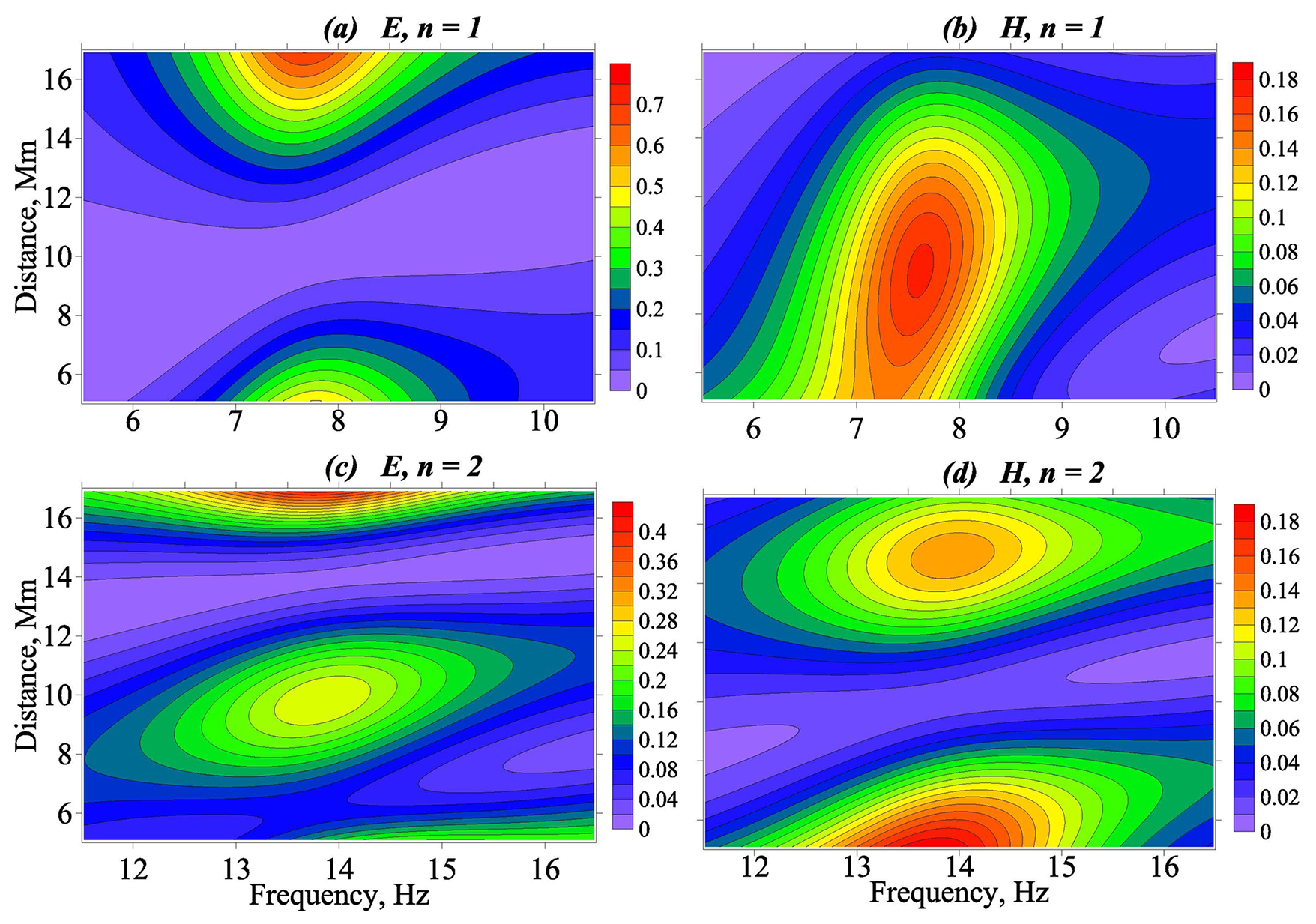
Figure 1 Distribution of the field intensities $|E_r{|}^{\mathrm{2}}$ and $|H_{\mathit{\phi }}{|}^{\mathrm{2}}$ of the first and the second SR modes over the frequency-distance plane.

This figure contains four maps showing the intensity distributions of the resonance field oscillations over the frequency-distance plane. The left panels of the figure depict the intensity of oscillations of the vertical electric field component $|E_r{|}^{\mathrm{2}}$. The right panels correspond to the power spectra of the total horizontal magnetic field $|H\mathit{\phi }{|}^{\mathrm{2}}$. The upper panels (Fig. 1a and b) show the intensity distributions of the first mode oscillations, and the lower panels (Fig. 1c and d) depict the corresponding intensity maps for the second mode oscillations. The specific field amplitudes in the unit frequency band were measured in mV m⁻¹ and µA m⁻¹, provided that the source current moment is equal to 10⁸ A m. The frequency in Hertz of radio signal is plotted along the horizontal axis at each map. The upper panels cover the band $\mathrm{5.5}<f<\mathrm{10.5}$ Hz (the vicinity of the first SR mode, n=1). The lower panels span the range $\mathrm{11.5}<f<\mathrm{16.5}$ Hz (the second SR mode, n=2). The distance D from the point vertical dipole source to the observer is plotted along the vertical axes of the maps measured in megameters (1 Mm = 1000 km). The intensity of resonant oscillations is presented by color, with the color scales placed to the right of the maps. The violet-blue palette corresponds to the low-level intensity, while the yellow-red colors correspond to the high-level oscillations.

For the first-mode magnetic field component (Fig. 1b) and the second-mode vertical electric field component (Fig. 1c), the intensity maximum occupies the area near the source-observer distance D=10 Mm. The outline of this maximum is asymmetric with respect to the vertical (distance) axis, indicating that the peak frequencies of the first mode in the magnetic field and of the second mode in the electric field gradually increase with the source–observer distance D. This monotonic behavior enables the estimation of the distance from an observer to the field source using the measured peak frequency.

In contrast, the first-mode vertical electric field component (Fig. 1a) and the second-mode magnetic field component (Fig. 1d) exhibit an intensity minimum near D≈10 Mm. This region is called the field nodal zone, which appears as an inclined violet band in the central part of the corresponding frequency-spatial distributions. Within this zone, the resonant intensity is strongly reduced, making it impossible to measure the peak frequencies there.

The nodal zone is also asymmetric with respect to the distance axis. Because the resonance peak vanishes in the nodal zone, the frequency experiences a discontinuity when crossing the 10 Mm distance. As the source distance increases within the D<10 Mm range, approaching the nodal zone, the peak frequency of the corresponding mode initially increases before the resonant peak disappears at D=10 Mm. Beyond the nodal zone (D>10 Mm), the intensity maximum reappears at lower frequencies and then gradually drifts toward higher frequencies as the distance continues to grow (see also Nickolaenko and Hayakawa, 2002, Fig. 4.20).

Crossing of the nodal line by a moving source causes a discontinuity in the distance dependence of the peak frequency, f(D), for a certain mode. Therefore, the distance dependence of the peak frequency is initially described by a convex curve, and transitions into concave curve after crossing the nodal line (Madden and Thompson, 1965; Jones, 1969; Galejs, 1970). This behavior arises from the interference of adjacent resonance modes, as described in detail in Sect. 4.1.5 of Nickolaenko and Hayakawa (2002).

In reality, global lightning activity is not point-like. It is typically concentrated over a confined tropical region. Consequently, the corresponding point field sources become distributed along the source–observer distance D. This spatial averaging smoothes the size of the f(D) discontinuity, replacing it with a rapid but finite frequency change. The wider is the region occupied by the field sources, the smaller the frequency variation (Jones, 1969, 1999; Galejs, 1970, 1972). This property allows for estimating the effective size of the zone occupied by thunderstorms using the observed diurnal range of frequency variations.

The frequency-distance distributions similar to the one depicted in Fig. 1a, are used to estimate the effective width of the area covered by global thunderstorm activity by analyzing the diurnal range of frequency variations (DFR) (Nickolaenko and Rabinowicz, 1995; Nickolaenko et al., 1998; Sátori et al., 2012, 2024; Nickolaenko and Hayakawa, 2002, 2014). The map of Fig. 1b might be used to estimate the diurnal changes in the source-receiver distance, D (Koloskov et al., 2013, 2020, 2022). Therefore, simultaneous records of the first SR mode frequency in the vertical electric and the horizontal magnetic fields allow deriving both the distance to the source and its effective size. The graphs on the lower panel in Fig. 1 indicate that this problem could also be successfully solved using simultaneous records of the first and second SR frequencies either in only the electric or only the magnetic fields.

Thus, we may conclude that the experimental SR studies have so far exploited only a half of their potential. Indeed, the long-term monitoring of the effective source width has been successfully conducted based on the DFR of the first mode frequency in the E_r field component (Sátori et al., 2024; Nickolaenko, 2024). Similarly, registrations of the source–observer distance (D) were successful using the first SR mode frequency in the H_φ field component (Koloskov et al. 2013, 2020, 2022, 2024). Unfortunately, the studies that provide both the source-observer distance (D) and the source effective size (W) remain desired.

The maps in Fig. 1 relevant to magnetic field are of special practical interest because most of operational SR observatories monitor the horizontal magnetic field. Within these observations, the resonance frequency of the first SR mode might be used to estimate the average source-observer distance (which is done successfully in practice), while the frequency of the second SR mode can be used to estimate the source effective size. Similarly, recording the first and the second SR frequencies in the vertical electric field will allow for estimating both the source size (W) and the source–observer distance (D). It should be noted that using the second electric mode has limitations due to secondary nodal zones at shorter and longer distances (e.g., Sátori et al., 2024). Thunderstorm activity in these additional nodal zones can affect the observed peak frequencies. However, this limitation is less critical for high-latitude stations like UAS “Akademik Vernadsky”, where distances to the main tropical thunderstorm centers mostly stay within the optimal 7–12 Mm range.

In the following section, we focus on the horizontal magnetic field measurements, performing the necessary calculations for a realistic model of the Earth – ionosphere cavity to obtain the calibration curves required for finding both the source – observer distance, D and the effective source width, W.

3 Calibration Curves

We perform the model computations and derive the calibration curves for the Ukrainian Antarctic station (UAS) “Akademik Vernadsky” (geographic coordinates: 65.35° S; 64.25° W), which hosts one of the longest series of SR observations worldwide (and the longest continuous record in the polar regions). At this site, two orthogonal horizontal magnetic field components H_WE and H_SN are recorded. We previously established the calibration curve for this site linking the peak frequency $f_{\mathrm{1}}^H$ of the first SR mode to the source-observer distance D, which was used to estimate the source dynamics (Nickolaenko et al., 2025a). Here we extend this approach by obtaining a formal relationship W (d$f_{\mathrm{2}}^H$) between the effective width of the field source W [in hour] and the diurnal frequency range (DFR) − d$f_{\mathrm{2}}^H$ (in Hz) of the second SR mode in the magnetic field records.

By using the graphs presented in Appendix A in Fig. A3, we derive the maximum (f^MAX) and the minimum (f^MIN) values of the second SR frequency in the magnetic component as functions of the source diameter W. These curves are shown in an inset of Fig. 2. They allow us to establish the calibration curve that links the DFR, defined as df = f^MAX−f^MIN with the source width W. The resulting d$f_{\mathrm{2}}^H$(W) curve is presented in the main plot of Fig. 2. Here, the vertical axis depicts the logarithm of the source width ln(W) (W is measured in hours: 1 h = $\mathit{\pi }/\mathrm{12}$ radians). The horizontal axis shows the logarithm of diurnal frequency range ln(d$f_{\mathrm{2}}^H$) (d$f_{\mathrm{2}}^H$ is measured in Hertz). The inset illustrates, on linear scale, the dependence of the daily maximum (red line with dots) and the minimum values (blue line with dots) of the second peak frequency versus the diameter W of the area covered by lightning strokes.

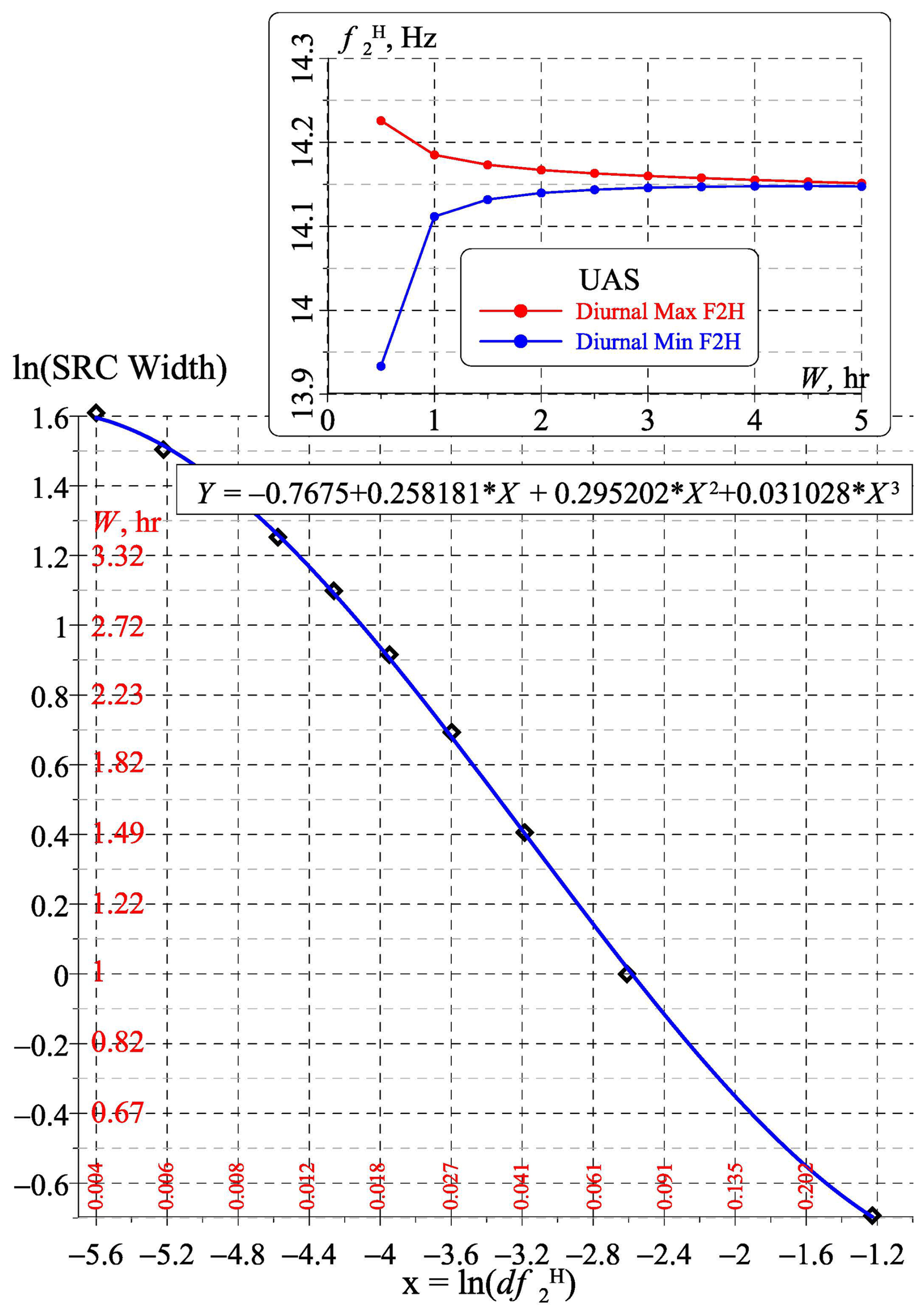
Figure 2 Calibration curve connecting the logarithm of the source width with the logarithm of the DFR of the second SR mode while measured at the Vernadsky station.

The computed calibration curve is shown in Fig. 2 by diamonds connected by a thin broken line. The pale green line shows the result of a polynomial fit of the X and Y logarithmic variables. This approximation is characterized by a high determination coefficient squared of R²=0.9997. The thick blue line depicts the calculated approximation that incorporates six significant digits in the fitting formula, presented as third degree polynomial:

$$\begin{array}{}\text{(1)}& \begin{array}{rl}Y& =-\mathrm{0.7675}+\mathrm{0.258181}\cdot X+\mathrm{0.295202}\cdot X^{\mathrm{2}}\\ & +\mathrm{0.031028}\cdot X^{\mathrm{3}},\end{array}\end{array}$$

where $X=\ln \left(\mathrm{d}{f}_{\mathrm{2}}^H\right)$ and $Y=\ln \left(\mathrm{d}{f}_{\mathrm{2}}^H\right)$.

Equation (1) enables the calculation of the diameter of the effective global thunderstorm activity zone (in hours) using the experimentally measured DFR of the second SR mode in the horizontal magnetic field component d$f_{\mathrm{2}}^H$.

For reference, we recall here the existing calibration equation that links the source – observer distance D and the peak frequency $f_{\mathrm{1}}^H$ of the first SR mode in the magnetic field (Koloskov et al., 2020):

$$\begin{array}{}\text{(2a)}& D=\mathrm{4.05784}\cdot {\mathrm{10}}^{-\mathrm{12}}\cdot (f_{\mathrm{1}}^H{)}^{\mathrm{13.8448}},\end{array}$$

or, equivalently

$$\begin{array}{}\text{(2b)}& \ln \left(D\right)=\mathrm{13.8448}\cdot \ln \left(f_{\mathrm{1}}^H\right)-\mathrm{26.2303}\mathrm{m},\end{array}$$

Taking together Eq. (1) (using d$f_{\mathrm{2}}^H$) and Eqs. (2a), (2b) (using $f_{\mathrm{1}}^H$) enables us to retrieve both the mean source–observer distance (D) and the effective source (W) width from horizontal magnetic-field observations.

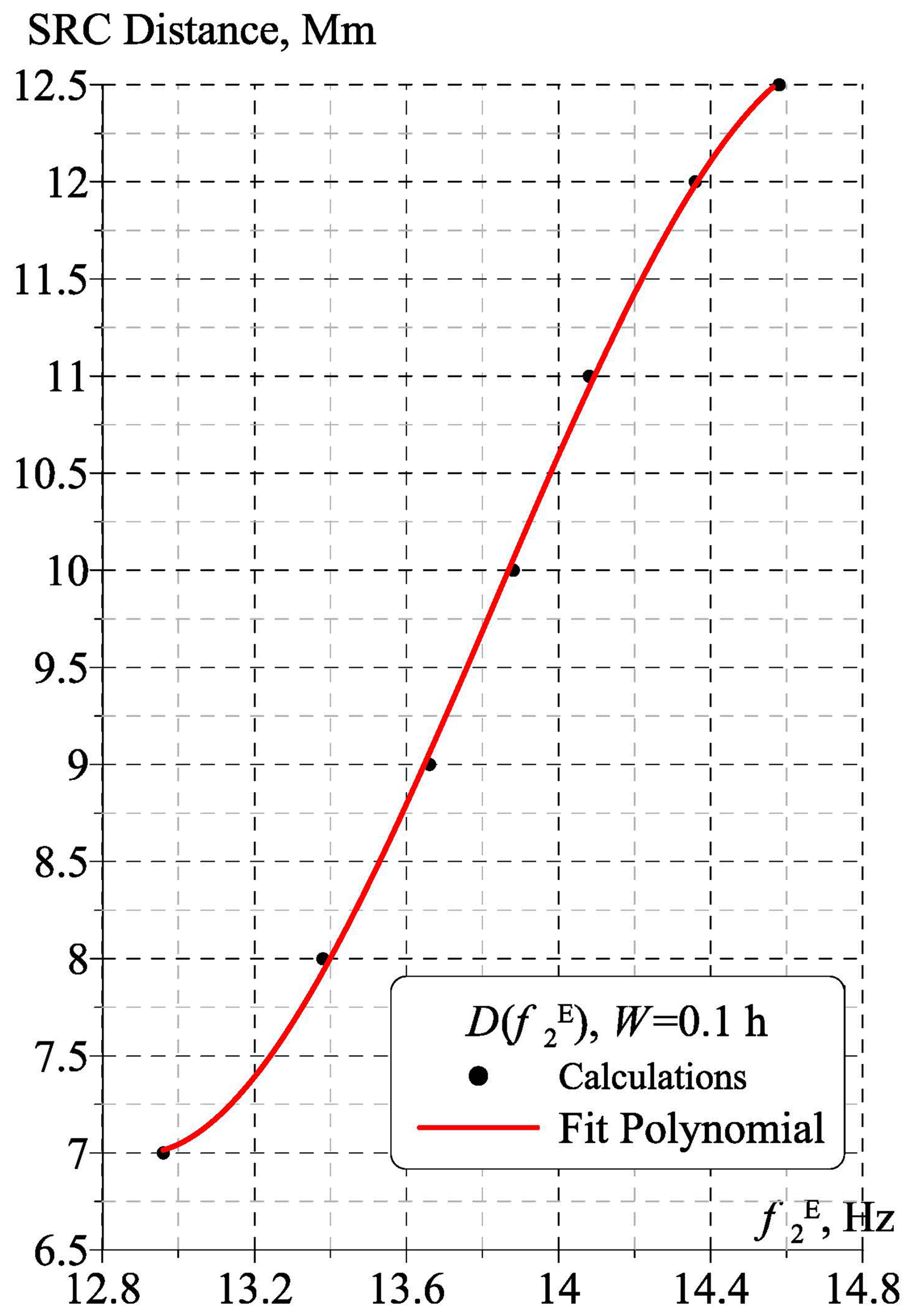
Figure 3 Calibration dependence D($f_{\mathrm{2}}^E$) for determining the source-observer distance, D from the second SR mode frequency in the vertical electric field while measured at the Vernadsky station.

It remains to provide a calibration formula that allows for estimating the average distance D from an observer to the global thunderstorms by using the records of the second SR mode in the electric field component. After performing the appropriate calculations simulating the observations at Vernadsky station, we obtain the data plotted in Fig. 3. The thin broken line with dots in this figure presents the calculated results, and the thick red curve shows the results of a third degree polynomial fit:

$$\begin{array}{}\text{(3)}& \begin{array}{rl}D& =\mathrm{4581.34}-\mathrm{1000.65}\cdot f_{\mathrm{2}}^E+\mathrm{72.5746}\cdot {\left(f_{\mathrm{2}}^E\right)}^{\mathrm{2}}\\ & -\mathrm{1.75139}\cdot {\left(f_{\mathrm{2}}^E\right)}^{\mathrm{3}},\end{array}\end{array}$$

where D the distance [in Mm] and $f_{\mathrm{2}}^E$ is the second-mode peak frequency [in Hz] in the vertical electric field. The determination coefficient squared for this fit is R²=0.9994.

For completeness, we reference the calibration dependence, which connects the effective source width W with the DRF in the first SR mode of vertical electric field d$f_{\mathrm{1}}^E$ (Nickolaenko, 2024)

$$\begin{array}{}\text{(3a)}& \ln \left(W_E\right)=-\mathrm{0.587}\cdot \ln \left(\mathrm{d}{f}_{\mathrm{1}}^E\right)+\mathrm{0.3216},\end{array}$$

or

$$\begin{array}{}\text{(3b)}& W_E=\mathrm{1.37935}\cdot {\left(\mathrm{d}{f}_{\mathrm{1}}^E\right)}^{-\mathrm{0.587}},\end{array}$$

The relevant coefficient of determination is R²=0.997. Equations (3a) and (3b) reflect the baseline analytical relation between the diurnal frequency range of the first electric mode and the global source size derived within a uniform Earth-ionosphere cavity model (Nickolaenko, 2024). Due to the fundamental spatial symmetry of the uniform resonator model, this analytical relation provides a robust baseline calibration applicable to both mid-latitude and high-latitude observatories as a primary approximation.

4 Conclusions

We derived and presented a complete set of calibration equations designed for processing SR observations conducted at the Ukrainian Antarctic Station (UAS) “Akademik Vernadsky”. Specifically, we provided formulas for determining the average distance D, to the center of global thunderstorm activity using either the contemporary frequency of the second SR mode in the vertical electric field E_r or first SR mode frequency in the horizontal field H_φ. Furthermore, we derived the equations that allow for calculating the effective size W, of the global thunderstorm area using the diurnal frequency range DFR of the first SR mode in the E_r component and/or the DFR of the second SR mode frequency in the H_φ field. These established relationships enable retrieval of both D and W from magnetic SR records at Vernadsky, supporting the comprehensive monitoring of the spatial distribution and extent of global lightning activity. For the European mid-latitude Nagycenk Observatory (Sátori et al., 2005), it would be desirable to update the site-specific calibration curve and its analytical fit. Finally, we conclude that this robust methodology is transferable to any other SR observatory worldwide.

Appendix A

Below we outline the model of the Earth-ionosphere cavity resonator used in this study. The atmosphere is represented as homogeneous and horizontally stratified, with the conductivity profile shown in Fig. A1. The tabular data (logarithm of conductivity – log(σ) versus height – h) corresponding to this profile can be found in Nickolaenko at al. (2025b).

Figure A1 Vertical profile of the middle atmosphere conductivity.

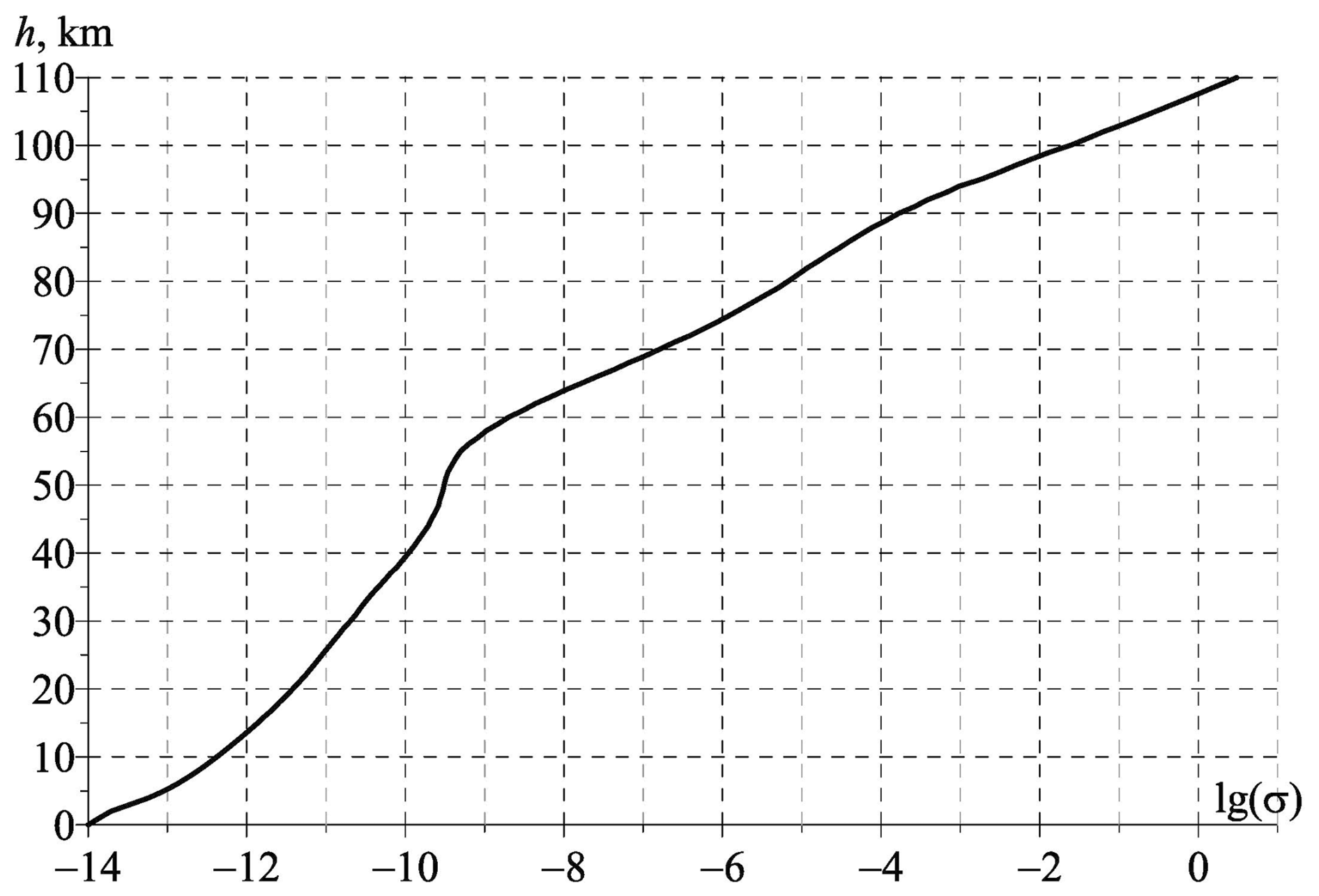
The conductivity profile in the middle atmosphere adopted here is based on the experimental observations of the Earth-ionosphere electromagnetic fields in the ELF (3 Hz–3 kHz) and ULF ($\mathrm{3}\times {\mathrm{10}}^{-\mathrm{3}}$–3 Hz) bands (see, e.g. Rycroft et al., 2025). The formal solution of the SR problem related to the atmospheric conductivity profile is well established (Madden and Thompson, 1965; Hynninen and Galuk, 1972; Bliokh et al., 1980; Jones and Knott, 1999). Using the conductivity-versus-height dependence, σ(h), one calculated the profile of the complex permittivity of the air. This is then used to compute the “radio technical” parameters of the Earth-ionosphere cavity: the propagation constant of ELF radio waves ν(f) and the complex characteristic heights of the ionosphere: the electric h_C(f) and the magnetic h_L(f) (Madden and Thompson, 1965; Greifinger and Greifinger, 1978). This part of the problem is solved using the full wave solution, specifically employing the Riccati equation (Hynninen and Galuk, 1972; Galuk, 2016). The frequency-dependent functions, thus obtained, are then substituted into the formal solution of the SR problem, which is expressed as the zonal harmonic series (Jones, 1999; Nickolaenko and Hayakawa, 2002, 2014).

Figure A2 presents the computational results for the parameters of the Earth-ionosphere cavity corresponding to the conductivity profile shown in Fig. A1.

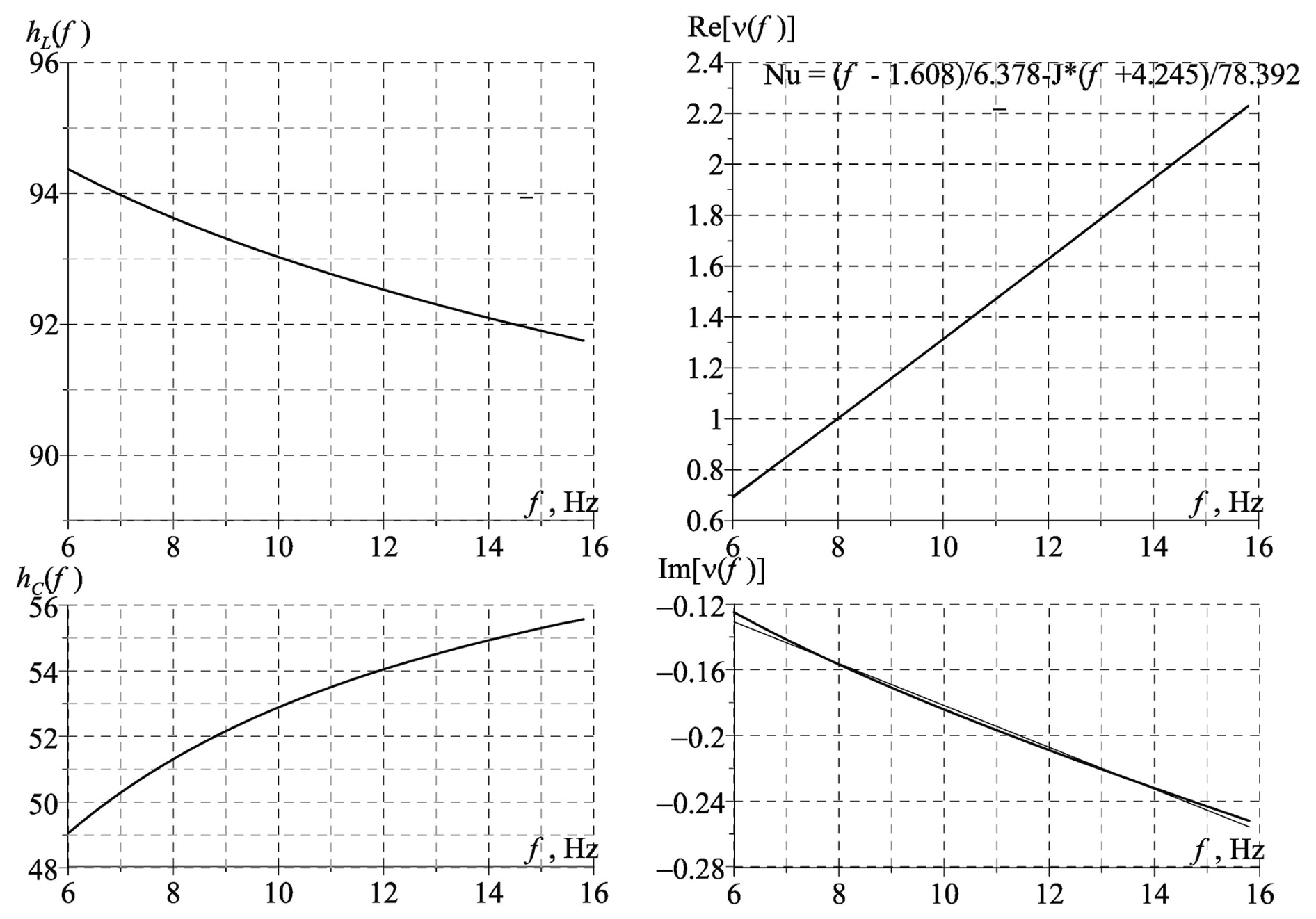
Figure A2 Real parts of the complex characteristic ionosphere heights (the graphs in the left column) and the complex propagation constant of ELF radio waves as a function of frequency (graphs in the right column).

The two left panels of Fig. A2 show the real parts of the magnetic and the electric characteristic heights (h_C and h_L) in the ionosphere against the frequency in the vicinity of the first and the second SR modes. The right panels of Fig. A2 show the frequency dependence of the real and imaginary parts of the complex propagation constant ν(f) or the dispersion function. The frequency variations of this parameter were approximated by the relation:

$$\begin{array}{}\text{(A1)}& \mathit{\nu }={\displaystyle \frac{f-\mathrm{1.608}}{\mathrm{6.378}}}-i\cdot {\displaystyle \frac{f+\mathrm{4.245}}{\mathrm{78.392}}}.\end{array}$$

The formula is used in numerical calculations. The formal solution of a problem for the vertical electric and horizontal magnetic fields is equal to:

$$\begin{array}{}\text{(A2)}& {\displaystyle }{E}_r\left(\mathit{\omega }\right)={\displaystyle \frac{\mathrm{1}}{\mathrm{4}{a}^{\mathrm{2}}\mathit{ϵ}{h}_C}}{\displaystyle \frac{i\mathit{\nu }\left(\mathit{\nu }+\mathrm{1}\right)}{\mathit{\omega }}}{\displaystyle \frac{P_{\mathit{\nu }}\left[\cos \left(\mathit{\pi }-\mathit{\theta }\right)\right]}{\sin \mathit{\pi }\mathit{\nu }}},\text{(A3)}& {\displaystyle }{H}_{\mathit{\phi }}\left(\mathit{\omega }\right)=-{\displaystyle \frac{\mathrm{1}}{\mathrm{4}a{h}_L\sin \mathit{\pi }\mathit{\nu }}}{\displaystyle \frac{\partial P_{\mathit{\nu }}\left[\cos \left(\mathit{\pi }-\mathit{\theta }\right)\right]}{\partial \mathit{\theta }}}.\end{array}$$

Here, a is the Earth's radius; ϵ is the permittivity of the free space; h_C and h_L are the electric and magnetic characteristic heights found from the full wave solution; P_ν[cos(π−θ)] is the Legendre function of the complex index ν; and θ is the source – observer angular distance.

When computing the electromagnetic fields, we use the zonal harmonic series representation for the Legendre functions, employing an accelerated convergence technique (Nickolaenko and Hayakawa, 2002, 2014). The calculations use a finite size source model where the distance between the observer and the center of the source is time-dependent. The source diameter W was varied in computational runs, taking values of 0.1; 0.5; 1.0; …; 5 h. The angular measure of 1 h is equivalent to 15° or 1.666 Mm. When the Universal time t_U advances, the angular distance D [in rad] from the observer to the center of distributed thunderstorm activity changes according to the law:

$$\begin{array}{}\text{(A4)}& D={\cos }^{-\mathrm{1}}\left[\sin {\mathit{\theta }}_{\mathrm{0}}\cdot \cos \left({\displaystyle \frac{t_U-\mathrm{17}}{\mathrm{12}}}\mathit{\pi }-{\mathit{\psi }}_{\mathrm{0}}\right)\right].\end{array}$$

Here, θ₀ and ψ₀ are the observer's co-latitude and longitude in radians, respectively.

The source is modeled as an area centered on the equatorial point corresponding to 17:00 h local time. This area moves around the globe during a day, and hence, around the observatory, over the course of a day. The distances from the observer to the individual lightning strokes are distributed along a parabola with its apex at the central point on the equator while the width of this parabola at the “zero level” is equal to W. In a way, this is analogous to a uniform distribution of lightning strokes within a circle of diameter W.

The finite size of the area W was accounted for in the field intensity computations by summing the field intensities over nineteen point sources. These sources were distributed equidistantly along the source – observer arc, where the individual angular distances are equal to:

$$\begin{array}{}\text{(A5)}& {\mathit{\theta }}_k=D-{\displaystyle \frac{W}{\mathrm{2}}}+k{\displaystyle \frac{W}{\mathrm{19}}},k\in \left[\mathrm{0},\mathrm{19}\right].\end{array}$$

The power spectrum of a particular field component ${\left|H_{\mathit{\phi }}\right|}^{\mathrm{2}}\sim {\left|\frac{\partial }{\partial \mathit{\theta }}{P}_{\mathit{\nu }}\left[\cos \left(\mathit{\pi }-{\mathit{\theta }}_k\right)\right]\right|}^{\mathrm{2}}$ or ${\left|E_r\right|}^{\mathrm{2}}\sim {\left|\mathit{\nu }(\mathit{\nu }+\mathrm{1})P_{\mathit{\nu }}\left[\cos \left(\mathit{\pi }-{\mathit{\theta }}_k\right)\right]\right|}^{\mathrm{2}}$ was computed for every of these distances θ_k. Afterwards, these power spectra were summed with the individual weights A_k:

$$\begin{array}{}\text{(A6)}& A_k=\mathrm{1}-\mathrm{4}{\left({\displaystyle \frac{{\mathit{\theta }}_k-D}{W}}\right)}^{\mathrm{2}}.\end{array}$$

For a fixed source width, the total spectra were computed as functions of Universal time t_U. Using these cumulative spectra relevant to the source of a specific size, we determine the resonance frequencies and their daily maximum and minimum values for each hour of Universal time. The resonance frequencies were calculated using the Rice (1944, 1945) formula:

$$\begin{array}{}\text{(A7)}& f_{\mathrm{Peak}}={\left[{\displaystyle \frac{{\int }_{f_L}^{f_h}{f}^{\mathrm{2}}S\left(f\right)\mathrm{d}f}{{\int }_{f_L}^{f_h}S\left(f\right)\mathrm{d}f}}\right]}^{\mathrm{1}/\mathrm{2}}.\end{array}$$

Here, S(f) denotes the power spectrum density of the horizontal magnetic or the vertical electric field. The integration limits were set as f_L=6.3 and f_H=9.3 Hz for the first SR mode, and f_L=12.5 and f_H=15.5 Hz for the second resonant mode. The frequency step used in numerical calculations involving Eq. (A7) was 0.1 Hz.

As expected, the calculated peak frequencies and their diurnal variations depend on the source width W, as demonstrated in Fig. A3. The Universal time [in hours] is plotted along the abscissa in Fig. A3, while the ordinate indicates the resonance frequency of the second SR mode in the magnetic field component. Curves of different colors correspond to different source widths W, as detailed in the lower right legend. Clearly, the DFR noticeably decreases with an increasing size of the area occupied by the global lightning activity. Since the center of this area located at 17:00 local time, and the observer's longitude is 64.25° W, the distance from the observer to the source center reaches its minimum value of approximately 7.14 Mm, around 06:00 Universal time. At 18:00 Universal time, this distance reaches the maximum value of approximately 12.86 Mm. When t_U=12 or 24 h, the source – observer distance is equal to 10 Mm.

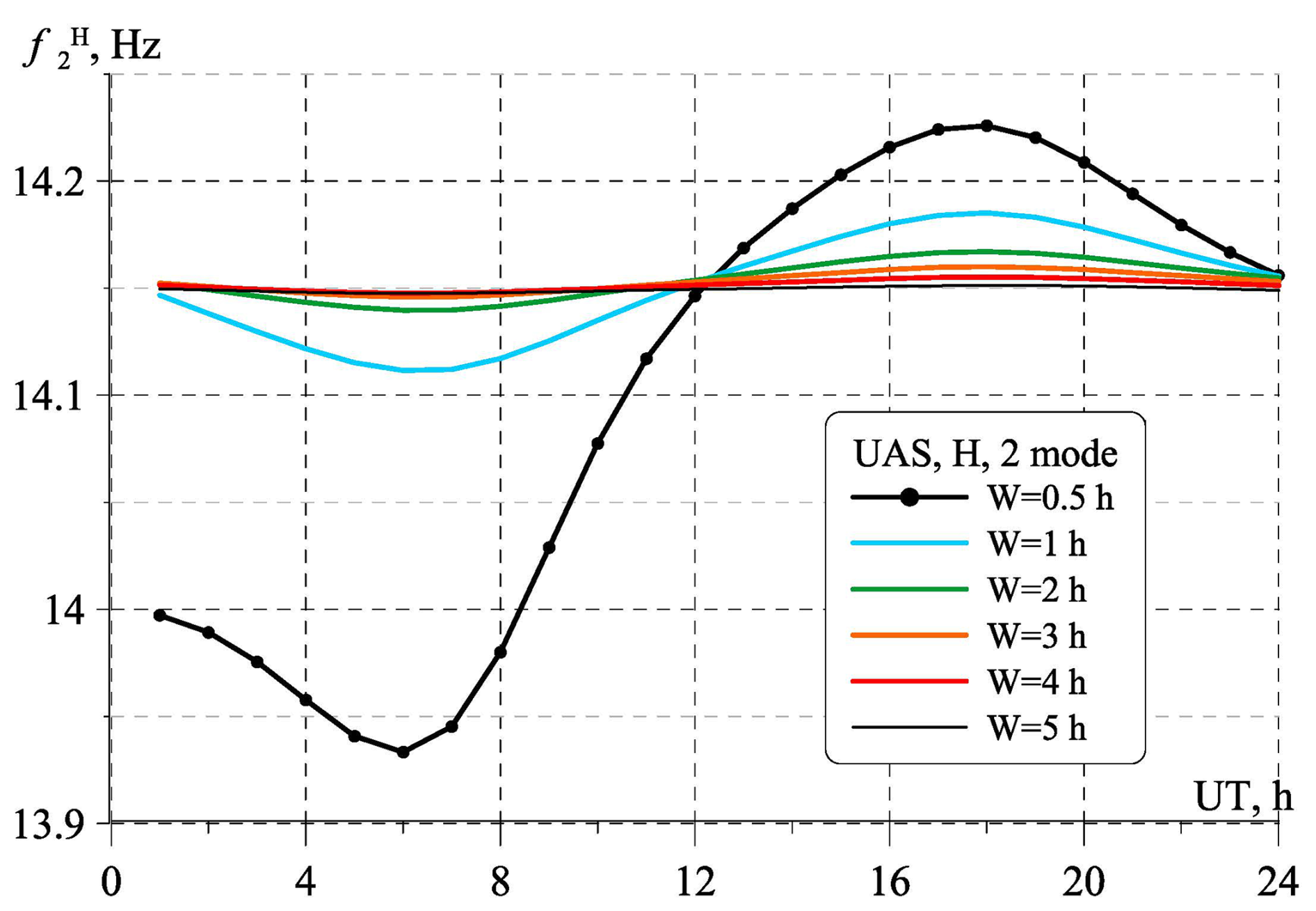
Figure A3 Impact of the source width on the range of diurnal variations in the second mode frequency in the horizontal magnetic field while measured at the Vernadsky station.

Our objective is to estimate for the size of zone occupied by the field sources. The curves in Fig. A3 provide the required link between the diurnal frequency range of the second SR mode recorded in the magnetic field and W. Using this result, we calculate the calibration curve shown in Fig. 2 of this paper.