Non-Maxwellian electron distributions in the D region during artificial heating – Part 1: Model development and electron temperature

The phase space density in the weakly ionized D region is calculated by numerically solving the Boltzmann equation and through a Monte Carlo simulation for high power, high frequency radio wave heating under the assumption that the electron collision frequency is much larger than the gyro-frequency. The effects of elastic and inelastic collisions, such as vibrational, rotational and electronic excitation, are taken into account using the best available cross sections. The solutions demonstrate that the distribution function deviates significantly from a Maxwellian distribution, and that even though a temperature can be defined from the second moment of the distribution, it is not sufficient to specify the distribution functions.

1 Introduction

The electron phase space density in the ionosphere is significantly modified by electron-neutral collisions. In the low-ionized D region with typical $N_{\mathrm{e}}/N_{\mathrm{n}}\approx$ 10⁻⁸–10⁻¹⁰, the electron-neutral collision frequency is typically larger than both the plasma and -gyro-frequency, and dominate and suppress collective plasma behaviour. When modelling the fluid behaviour of the ionospheric plasma, for example electron heating and cooling, absorption and refraction of radio waves and D region chemistry, the standard simplifying assumption is that the electron distribution remain Maxwellian. The benefit of this assumption is that it becomes straightforward to calculate macroscopic properties of the electron gas, such as heat capacity and cooling rates (Pavlov, 1998a, b; Pavlov and Berrington, 1999; Campbell et al., 2004), collision frequency and refractive index, and chemical reaction rates (e.g. Turunen et al., 1996; Viehland and Johnsen, 2018).

However, the electron distribution can differ significantly from a Maxwellian when the electrons are significantly heated; for example under the influence of powerful high frequency (HF) radio waves. Artificial heating in the D region increases the electron temperature due to Ohmic heating, where the radio wave heats the electrons by absorbing radio wave energy. Both elastic and inelastic collisions interrupt the collective electron oscillation driven by the electric field of the radio wave. Elastic collisions lead to a random change in the direction of the electron velocity. This increases the thermal energy of the electrons and thereby raises the electron temperature. Inelastic collisions, though less frequent than elastic collisions, reduce the energy of the electrons due to excitation of neutrals, wherein the electrons lose the excitation energy. Electrons that have gained enough energy to excite vibrational states in molecular nitrogen (N₂) are of particular interest, as these states have large cross sections in the energy range from 2 to 3.5 eV. In combination, the above-mentioned processes tend to make the electron velocity distribution non-Maxwellian during HF radio wave propagation through the ionospheric plasma, as previously shown by e.g., Carleton and Megill (1962); Mintzer (1964); Gurevich (1978); Stubbe (1981); Gustavsson et al. (2004).

In this and the accompanying paper (Myrvang and Gustavsson, 2026b), we study the deviation from a Maxwellian and its impact on electron cooling rates. This paper, referred to as Part 1, presents updated methods for calculating the electron phase space density in a low-ionized plasma, and our result illustrate how the standard Maxwellian temperature can become misleading. The accompanying paper, Part 2, study how the deviation from a Maxwellian influence the macroscopic properties of the electron gas, presenting electron cooling rates for vibrational excitation of N₂ and molecular oxygen (O₂), as well as the excitation of fine structure levels in atomic oxygen (O). To achieve this, we have implemented methods to calculate non-Maxwellian electron velocity distributions for a weakly ionized plasma at D region heights during artificial heating. These methods are based on kinetic theory, adapted from Stubbe (1981), and a Monte Carlo simulation where the electron equation of motion is solved with forcing from a HF radio wave electric field between collisions. The aim of Part 1 is to update the kinetic method by Stubbe (1981). Here, our contribution include the use of the best available measured or theoretical cross section for the excitation of vibrational states of N₂ and O₂ and the excitation of fine structure levels of O. Our results demonstrate that that the standard method for calculating the electron temperature becomes problematic when the distribution deviates significantly from a Maxwellian.

The paper is organized as follows: Sect. 2 introduces the numerical solution of Boltzmann equation, while Sect. 3 provides an account on the Monte Carlo simulation, and Sect. 4 briefly introduces the concept of electron temperature. Section 5 presents the results, Sect. 6 discusses the results and Sect. 7 summarize the study.

2 Numerical solution of the Boltzmann equation

The evolution of the electron phase space density, $f(\mathit{r},\mathit{v},t)$, is described by the Boltzmann equation (e.g. Schunk et al., 2018):

$$\begin{array}{}\text{(1)}& \begin{array}{rl}{\displaystyle \frac{\partial }{\partial t}}f(\mathit{r},\mathit{v},t)& +(\mathit{v}\cdot {\mathbf{\nabla }}_{\mathit{r}})f(\mathit{r},\mathit{v},t)\\ & +\left[{\displaystyle \frac{\mathit{F}}{m}}\cdot {\mathbf{\nabla }}_{\mathit{v}}\right]f(\mathit{r},\mathit{v},t)={\left({\displaystyle \frac{\partial f}{\partial t}}\right)}_{\text{coll}}\end{array}\end{array}$$

where $f(\mathit{r},\mathit{v},t)$ varies in time due to the electron's non-zero velocity, external forces acting on the electrons and collisions between electron and neutrals or ions. For the D region, we can assume a homogenous, cold, weakly ionized plasma. Since the neutral density is significantly higher than the electron density in the D region, with typical ionization fraction of 10⁻¹²–10⁻⁸, electron-neutral collisions dominate over electron-electron and electron-ion collisions. Therefore, we can neglect the effects of these collisions. In addition, we neglect the influence of Earth's magnetic field since the electron-neutral collision frequency is much higher than the electron gyro-frequency ω_c, which implies that the electrons are unlikely to complete a gyro-orbit between collisions. For external forces, we assume that an artificial heating radio wave with an oscillating electric field acts on the electrons:

$$\begin{array}{}\text{(2)}& \mathit{E}=E_{\mathrm{0}}{\mathit{e}}_{\mathit{x}}\cos \left(\mathit{\omega }t\right)\end{array}$$

where E₀ is the amplitude of the electric field and ω is the angular frequency of the radio wave. With our assumptions for the D region, the Boltzmann equation simplifies to:

$$\begin{array}{}\text{(3)}& {\displaystyle \frac{\partial f}{\partial t}}+\mathit{\gamma }\cos \left(\mathit{\omega }t\right){\displaystyle \frac{\partial f}{\partial v_x}}={\left({\displaystyle \frac{\partial f}{\partial t}}\right)}_{\text{el}}+{\left({\displaystyle \frac{\partial f}{\partial t}}\right)}_{\text{ie}}\end{array}$$

where f(v,t) is the distribution function in velocity space, γ is the electron acceleration by the heating wave $\mathit{\gamma }=-q_{\mathrm{e}}{E}_{\mathrm{0}}/m_{\mathrm{e}}$, −q_e is the elementary charge of an electron and m_e is the electron mass. It is possible to determine f(v,t) by expansion in spherical harmonics with Legendre polynomials and Fourier series (Mintzer, 1964). Keeping only the first two terms in the expansion leads to:

$$\begin{array}{}\text{(4)}& \begin{array}{rl}f(\mathit{v},t)& =f_{\mathrm{0}}\left(v\right)+f_{\mathrm{1}}(v_x,v,t)\\ & =f_{\mathrm{0}}\left(v\right)+\mathit{\gamma }{v}_x\left[g_{\mathrm{1}}\right(v\left)\cos \right(\mathit{\omega }t)+h_{\mathrm{1}}(v\left)\sin \right(\mathit{\omega }t\left)\right]\end{array}\end{array}$$

Furthermore, following Stubbe (1981), we make the simplifying assumption that:

$$\begin{array}{}\text{(5)}& \begin{array}{rl}& {\left({\displaystyle \frac{\partial f}{\partial t}}\right)}_{\text{el}}+{\left({\displaystyle \frac{\partial f}{\partial t}}\right)}_{\text{ie}}\\ & \textcolor{red}{}\end{array}\end{array}$$

since f₀ is almost perfectly isotropic and elastic collisions only change the direction of the electron velocity, it follows that $(\partial f_{\mathrm{0}}/\partial t{)}_{\text{el}}=\mathrm{0}$. Furthermore, since elastic cross section are larger than inelastic cross sections, $(\partial f_{\mathrm{1}}/\partial t{)}_{\text{ie}}$ can be neglected. For the elastic collision integral, we follow Stubbe (1981):

$$\begin{array}{}\text{(6)}& {\left({\displaystyle \frac{\partial f_{\mathrm{1}}}{\partial t}}\right)}_{\text{el}}=-\mathit{\gamma }{v}_x\mathit{\nu }\left(v\right)\left[g_{\mathrm{1}}\right(v\left)\cos \right(\mathit{\omega }t)+h_{\mathrm{1}}(v\left)\sin \right(\mathit{\omega }t\left)\right]\end{array}$$

As in Stubbe (1981), we use an approximate expression from Phelps and Pack (1959) and Hake and Phelps (1967) for the electron-neutral collision frequency ν(v):

$$\begin{array}{}\text{(7)}& \mathit{\nu }\left(v\right)=b{N}_{\mathrm{n}}{v}^{\mathrm{2}}\end{array}$$

where v is the electron speed, $N_{\mathrm{n}}={\mathrm{N}}_{\mathrm{2}}+{\mathrm{O}}_{\mathrm{2}}+\mathrm{O}$, N₂ and O₂ are the number density of N₂ or O₂, respectively and O is the number density of O, and b = 2.8 × 10⁻²⁵ m s. The inelastic collision term consists of several parts: rotational excitation, vibrational excitation, electron excitation and excitation of fine structure levels of O. Rotational excitation can be simplified (Gurevich, 1978):

$$\begin{array}{}\text{(8)}& {\left({\displaystyle \frac{\partial f_{\mathrm{0}}}{\partial t}}\right)}_{\text{rot}}={\displaystyle \frac{\mathrm{4}{\mathit{\sigma }}_{\mathrm{0}}{B}_{\mathrm{0}}}{m_{\mathrm{e}}}}{N}_{\mathrm{n}\mathrm{2}}{\displaystyle \frac{\mathrm{1}}{v^{\mathrm{2}}}}{\displaystyle \frac{\partial }{\partial v}}\left[{\displaystyle \frac{k_b{T}_{\mathrm{n}}}{m_{\mathrm{e}}}}v{\displaystyle \frac{\partial f_{\mathrm{0}}}{\partial v}}+v^{\mathrm{2}}{f}_{\mathrm{0}}\right]\end{array}$$

where $N_{\mathrm{n}\mathrm{2}}={\mathrm{N}}_{\mathrm{2}}+{\mathrm{O}}_{\mathrm{2}}$, k_b is Boltzmann's constant, T_n is the neutral temperature and σ₀B₀ = 2.49 × 10²¹ kg m⁴ s⁻². For excitation of vibrational states, electronic states and fine structure levels, we only consider excitation from the ground state, which simplifies to:

$$\begin{array}{}\text{(9)}& \begin{array}{rl}{\left({\displaystyle \frac{\partial f_{\mathrm{0}}}{\partial t}}\right)}_{\text{ie}}=& {\displaystyle \frac{\mathrm{2}}{m_{\mathrm{e}}v}}\sum _l{N}_l\sum _{j=\mathrm{1}}^{\mathrm{\infty }}[-\underset{\text{loss\hspace{0.17em}\hspace{0.17em}from\hspace{0.17em}\hspace{0.17em}energy}}{\underbrace{E{f}_{\mathrm{0}}\left(E\right){\mathit{\sigma }}_l^j\left(E\right)}}E\\ & +\underset{\text{contribution\hspace{0.17em}\hspace{0.17em}at\hspace{0.17em} }E\mathit{\text{ \hspace{0.17em}from\hspace{0.17em}\hspace{0.17em}higher\hspace{0.17em}\hspace{0.17em}energies}}}{\underbrace{(E+\mathrm{\Delta }{E}_l^j)f_{\mathrm{0}}(E+\mathrm{\Delta }{E}_l^j){\mathit{\sigma }}_l^j(E+\mathrm{\Delta }{E}_l^j)}}]\end{array}\end{array}$$

where $\mathrm{\Delta }{E}_l^j$ is the excitation energy from the ground state to the state j with cross sections ${\mathit{\sigma }}_l^j$ for the neutral constituents N_l. The full expression, where excitation from all levels are included, is given in Appendix B. Next, to derive an expression for the distribution function, we insert the expansion of f(v,t) from Eq. (4) into the simplified Boltzmann Eq. (3), leading to:

$$\begin{array}{}\text{(10)}& \begin{array}{rl}& \textcolor{red}{}\\ & +\mathit{\gamma }\cos \left(\mathit{\omega }t\right){\displaystyle \frac{\partial f_{\mathrm{0}}}{\partial v_x}}\\ & +{\mathit{\gamma }}^{\mathrm{2}}\cos \left(\mathit{\omega }t\right)\left[g_{\mathrm{1}}\right(v\left)\cos \right(\mathit{\omega }t)+h_{\mathrm{1}}(v\left)\sin \right(\mathit{\omega }t\left)\right]\\ & +{\mathit{\gamma }}^{\mathrm{2}}\cos \left(\mathit{\omega }t\right)v_x\left[{\displaystyle \frac{\partial g_{\mathrm{1}}}{\partial v_x}}\cos \left(\mathit{\omega }t\right)+{\displaystyle \frac{\partial h_{\mathrm{1}}}{\partial v_x}}\sin \left(\mathit{\omega }t\right)\right]\\ =& {\left({\displaystyle \frac{\partial f_{\mathrm{1}}}{\partial t}}\right)}_{\text{el}}+{\left({\displaystyle \frac{\partial f_{\mathrm{0}}}{\partial t}}\right)}_{\text{ie}}\end{array}\end{array}$$

This equation is effectively a three term Fourier expansion of f with frequencies of 0 (DC-term), ω (the heating frequency) and 2ω (the second harmonic). For steady state condition, f₀ does not vary with time. We then proceed to equate the coefficient for each frequency component, which after some algebra results in:

$$\begin{array}{}\text{(11)}& -{\displaystyle \frac{\mathrm{1}}{\mathrm{6}}}{\displaystyle \frac{{\mathit{\gamma }}^{\mathrm{2}}}{v^{\mathrm{2}}}}{\displaystyle \frac{\partial }{\partial v}}\left[{\displaystyle \frac{\mathit{\nu }{v}^{\mathrm{2}}}{{\mathit{\omega }}^{\mathrm{2}}+{\mathit{\nu }}^{\mathrm{2}}}}{\displaystyle \frac{\partial f_{\mathrm{0}}}{\partial v}}\right]={\left({\displaystyle \frac{\partial f_{\mathrm{0}}}{\partial t}}\right)}_{\text{ie}}\end{array}$$

Multiplying Eq. (11) with 4πv² and $\mathrm{1}/N_{\mathrm{n}\mathrm{2}}$ and integrating from zero to v:

$$\begin{array}{}\text{(12)}& \begin{array}{rl}& -{\displaystyle \frac{{\mathit{\gamma }}^{\mathrm{2}}}{\mathrm{6}}}{\displaystyle \frac{\mathrm{1}}{N_{\mathrm{n}\mathrm{2}}}}\underset{\mathrm{0}}{\overset{v}{\int }}{\displaystyle \frac{\partial }{\partial v}}\left[{\displaystyle \frac{\mathit{\nu }{v}^{\mathrm{2}}}{{\mathit{\omega }}^{\mathrm{2}}+{\mathit{\nu }}^{\mathrm{2}}}}{\displaystyle \frac{\partial f_{\mathrm{0}}}{\partial v}}\right]\mathrm{d}v\\ =& {\displaystyle \frac{\mathrm{1}}{N_{\mathrm{n}\mathrm{2}}}}\underset{\mathrm{0}}{\overset{v}{\int }}{v}^{\mathrm{2}}{\left({\displaystyle \frac{\partial f_{\mathrm{0}}}{\partial t}}\right)}_{\text{ie}}\mathrm{d}v\end{array}\end{array}$$

We expand the right hand side by inserting expressions for the various inelastic excitations, simplify and multiply by $m_{\mathrm{e}}^{\mathrm{2}}$ and (4σ₀B₀vf₀)⁻¹, which gives:

$$\begin{array}{}\text{(13)}& \begin{array}{rl}& -{\displaystyle \frac{m_{\mathrm{e}}^{\mathrm{2}}b{r}_{\mathrm{N}}{\mathit{\gamma }}^{\mathrm{2}}}{\mathrm{24}{\mathit{\sigma }}_{\mathrm{0}}{B}_{\mathrm{0}}v}}\left[{\displaystyle \frac{v^{\mathrm{4}}}{{\mathit{\omega }}^{\mathrm{2}}+{\mathit{\nu }}^{\mathrm{2}}}}\right]{\displaystyle \frac{\mathrm{1}}{f_{\mathrm{0}}}}{\displaystyle \frac{\partial f_{\mathrm{0}}}{\partial v}}\\ =& k_b{T}_{\mathrm{n}}{\displaystyle \frac{\mathrm{1}}{f_{\mathrm{0}}}}{\displaystyle \frac{\partial f_{\mathrm{0}}}{\partial v}}+m_{\mathrm{e}}v+{\displaystyle \frac{m_{\mathrm{e}}^{\mathrm{2}}G\left(u\right)}{\mathrm{4}{\mathit{\sigma }}_{\mathrm{0}}{B}_{\mathrm{0}}v{f}_{\mathrm{0}}}}\end{array}\end{array}$$

where $r_{\mathrm{N}}=N_{\mathrm{n}}/N_{\mathrm{n}\mathrm{2}}$ and G(v) is defined as:

$$\begin{array}{}\text{(14)}& G\left(v\right)={\displaystyle \frac{\mathrm{1}}{N_{\mathrm{n}\mathrm{2}}}}\underset{\mathrm{0}}{\overset{v}{\int }}{v}^{\mathrm{2}}{\left({\displaystyle \frac{\partial f_{\mathrm{0}}}{\partial t}}\right)}_{\text{ie}}\mathrm{d}v\end{array}$$

G(v) describes the cumulative increase in phase space density at all speeds below v due to energy degradation from higher speeds. Therefore, G(v) will be zero-positive. Equation (13) can be rearranged to:

$$\begin{array}{}\text{(15)}& {\displaystyle \frac{\mathrm{1}}{f_{\mathrm{0}}}}{\displaystyle \frac{\partial f_{\mathrm{0}}}{\partial v}}=-\left({\displaystyle \frac{{\displaystyle }{m}_{\mathrm{e}}v+{\displaystyle \frac{m_{\mathrm{e}}^{\mathrm{2}}G\left(v\right)}{\mathrm{4}{\mathit{\sigma }}_{\mathrm{0}}{B}_{\mathrm{0}}v{f}_{\mathrm{0}}}}}{{\displaystyle }{k}_b{T}_{\mathrm{n}}+{\displaystyle \frac{m_{\mathrm{e}}^{\mathrm{2}}b{r}_{\mathrm{N}}{\mathit{\gamma }}^{\mathrm{2}}}{\mathrm{24}{\mathit{\sigma }}_{\mathrm{0}}{B}_{\mathrm{0}}}}{\displaystyle \frac{v^{\mathrm{3}}}{{\mathit{\omega }}^{\mathrm{2}}+{\mathit{\nu }}^{\mathrm{2}}}}}}\right)\end{array}$$

which can almost be solved as a first order separable differential equation. This would give the electron velocity distribution:

$$\begin{array}{}\text{(16)}& f_{\mathrm{0}}\left(v\right)=A\exp \left\{-{\displaystyle }\underset{\mathrm{0}}{\overset{v}{\int }}{\displaystyle \frac{{\displaystyle }{m}_{\mathrm{e}}v+{\displaystyle \frac{m_{\mathrm{e}}^{\mathrm{2}}G\left(v\right)}{\mathrm{4}{\mathit{\sigma }}_{\mathrm{0}}{B}_{\mathrm{0}}v{f}_{\mathrm{0}}\left(v\right)}}}{{\displaystyle }{k}_b{T}_{\mathrm{n}}+{\displaystyle \frac{m_{\mathrm{e}}^{\mathrm{2}}b{r}_{\mathrm{N}}{\mathit{\gamma }}^{\mathrm{2}}}{\mathrm{24}{\mathit{\sigma }}_{\mathrm{0}}{B}_{\mathrm{0}}}}{\displaystyle \frac{v^{\mathrm{3}}}{{\mathit{\omega }}^{\mathrm{2}}+{\mathit{\nu }}^{\mathrm{2}}}}}}\mathrm{d}v\right\}\end{array}$$

The normalization constant A is found by conserving the electron density N_e:

$$\begin{array}{}\text{(17)}& A={\displaystyle \frac{N_{\mathrm{e}}}{\mathrm{4}\mathit{\pi }\underset{\mathrm{0}}{\overset{\mathrm{\infty }}{\int }}{f}_{\mathrm{0}}\left(v\right)v^{\mathrm{2}}\mathrm{d}v}}\end{array}$$

The electron density is assumed to be 10¹⁰ m³, while height profiles for the neutral density are taken from MSISE-90 model (Hedin, 1991; Picone et al., 2002), and the neutral temperature is assumed 200 K. Since f₀ appears on both the LHS and inside the exponential on the RHS of Eq. (16), we solve it numerically with an iteration scheme starting from a Maxwellian distribution f₀(v)⁰:

$$\begin{array}{}\text{(18)}& f_{\mathrm{0}}(v{)}^{i+\mathrm{1}}=A\exp \left\{-\underset{\mathrm{0}}{\overset{v}{\int }}{\displaystyle \frac{{\displaystyle }{m}_{\mathrm{e}}v+{\displaystyle \frac{m_{\mathrm{e}}^{\mathrm{2}}G\left(f_{\mathrm{0}}\right(v{)}^i)}{\mathrm{4}{\mathit{\sigma }}_{\mathrm{0}}{B}_{\mathrm{0}}v{f}_{\mathrm{0}}(v{)}^i}}}{k_b{T}_{\mathrm{n}}+{\displaystyle \frac{m_{\mathrm{e}}^{\mathrm{2}}b{r}_{\mathrm{N}}{\mathit{\gamma }}^{\mathrm{2}}}{\mathrm{24}{\mathit{\sigma }}_{\mathrm{0}}{B}_{\mathrm{0}}}}{\displaystyle \frac{v^{\mathrm{3}}}{{\mathit{\omega }}^{\mathrm{2}}+{\mathit{\nu }}^{\mathrm{2}}}}}}\mathrm{d}v\right\}\end{array}$$

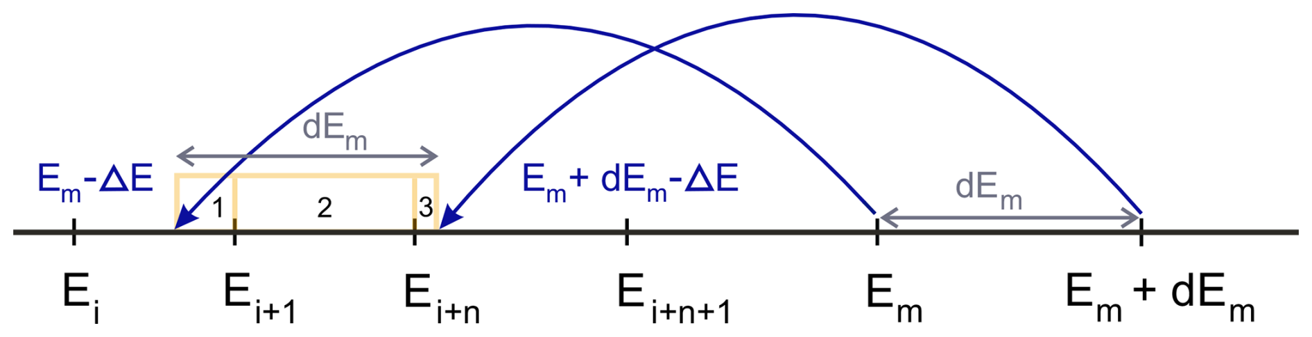
Figure 1 Electron degradation, where dE is energy resolution and ΔE is the excitation energy for the different types of inelastic collisions. We show electrons degrading from one energy bin with bin edges given by E_m(v_m) and E_m(v_m)+dE_m. The electrons lose energy according to the excitation energy and degrade to lower energy with bin edges E_m(v_m)−ΔE and $E_m\left(v_m\right)+{\text{dE}}_m-\mathrm{\Delta }E$.

When $f^i=f^{i+\mathrm{1}}$, then fⁱ⁺¹ solves Eq. (16). That the iteration scheme described in Eq. (18) converges is not guaranteed. However, with a slowed downed iteration in the form of:

$$\begin{array}{}\text{(19)}& f_{\mathrm{0}}(v{)}^{i+\mathrm{2}}=c_{\mathrm{s}}{f}_{\mathrm{0}}(v{)}^i+(\mathrm{1}-c_{\mathrm{s}})f_{\mathrm{0}}(v{)}^{i+\mathrm{1}}\end{array}$$

where c_s lies between 0 and 1, the convergence turns out to be more well-behaved. In our experience for ionospheric condition, this scheme converges well within 60 iterations.

To solve Eq. (16), one must account for inelastic collision, where electrons lose the excitation energy $\mathrm{\Delta }{E}_l^j$ of state j for neutral constituent l, thereby degrading to lower energies. This is achieved by computing the inelastic collision integral given in Eq. (9) for vibrational excitation, electronic excitation and excitation of fine structure levels. For elastic collisions between electrons and neutrals, as well as rotational excitation, we apply the approximated expressions from Eqs. (6) and (8), respectively. In this paper, a finite element representation of the phase space density f(v)d³v is used, together with cross sections that are continuous in energy. To accurately account for energy degradation of electrons losing energy ΔE from velocity bins $[v_m,v_m+\mathrm{d}v]$ with energies in the range $m_{\mathrm{e}}/\mathrm{2}[v_m^{\mathrm{2}},(v_m+\mathrm{d}v{)}^{\mathrm{2}}]$ to velocity bins covering energies between $m_{\mathrm{e}}/\mathrm{2}[v_m^{\mathrm{2}}-\mathrm{\Delta }E,(v_m+\mathrm{d}v{)}^{\mathrm{2}}-\mathrm{\Delta }E]$, we partition the contribution of the degrading electrons into the respective bins. Additionally, we carefully consider the misalignment between the velocity grid and the velocity limits of the degrading electrons, as illustrated in Fig. 1.

Our solution of the Boltzmann equations is rather similar to the one presented by Stubbe (1981). The main difference lies in our use of continuous cross sections for all inelastic processes, and the consequential partition of electrons into bins after collision. This approach contrasts with the discrete delta spike approach used by Stubbe (1981), where electrons at a discrete velocity degrade by the excitation energy to a discrete velocity with lower energy. Another distinction is our use of slightly different factors in Eq. (16), as the definitions provided in Eqs. (15) and (16) by Stubbe (1981) have incorrect units. For a detailed derivation of the electron velocity distribution, refer to Appendix B. See Stubbe (1981) for the original derivation.

3 Monte Carlo simulation

To validate our solution of the Boltzmann equation, a Monte Carlo simulation has been implemented. The simulation integrates the electron momentum equation with acceleration by an oscillating electric field of a HF-wave between collisions with neutrals, where the collision cross sections are taken from Gustavsson (2022). The time between collisions is drawn from exponentially distributed random numbers with expected values corresponding to the mean free path. Collisions are either elastic, leading to a change in direction without loss of energy, or inelastic with loss of energy. The scattering is assumed to be isotropic, which is a good approximation for electrons with energies below 5 eV (Brunger and Buckman, 2002; Dehmel et al., 1976). This procedure is repeated for 10⁶ electrons, starting with a thermal electron velocity distribution that fairly quickly becomes non-Maxwellian due to the combined effects of HF-heating and elastic and inelastic collisions. In this way, it is possible to observe the initial response of the electrons just after onset of HF-heating. The electrons are traced well into steady conditions. Note that the time required to reach steady state varies with altitude due to changes in the electron-neutral collision frequency.

4 Electron temperature

For a phase space density that differs significantly from a Maxwellian, defining an electron temperature is not straightforward. One way to characterize the electron temperature is by taking the second moment of the non-Maxwellian distribution:

$$\begin{array}{}\text{(20)}& T_{\mathrm{2}\text{nd}}={\displaystyle \frac{\mathrm{4}\mathit{\pi }}{\mathrm{3}}}{\displaystyle \frac{m_{\mathrm{e}}}{k_b}}\underset{\mathrm{0}}{\overset{\mathrm{\infty }}{\int }}{f}_{\mathrm{0}}\left(v\right)v^{\mathrm{4}}\mathrm{d}v/\mathrm{4}\mathit{\pi }\underset{\mathrm{0}}{\overset{\mathrm{\infty }}{\int }}{f}_{\mathrm{0}}\left(v\right)v^{\mathrm{2}}\mathrm{d}v\end{array}$$

which represents the total thermal energy in the electron gas. However, for a non-Maxwellian distribution, the phase space density varies with energy in a more complicated manner and to capture this, a more general “effective temperature” T_eff that varies with energy can be introduced (Gurevich et al., 1985):

$$\begin{array}{}\text{(21)}& T_{\text{eff}}\left(E\right)=-{\displaystyle \frac{f_{\mathrm{0}}\left(E\right)}{{\displaystyle \frac{d{f}_{\mathrm{0}}}{\text{dE}}}}}\end{array}$$

where f₀ is the non-Maxwellian distribution. Note that for a Maxwellian distribution, T_eff reduces to the standard electron temperature, which remains constant with energy.

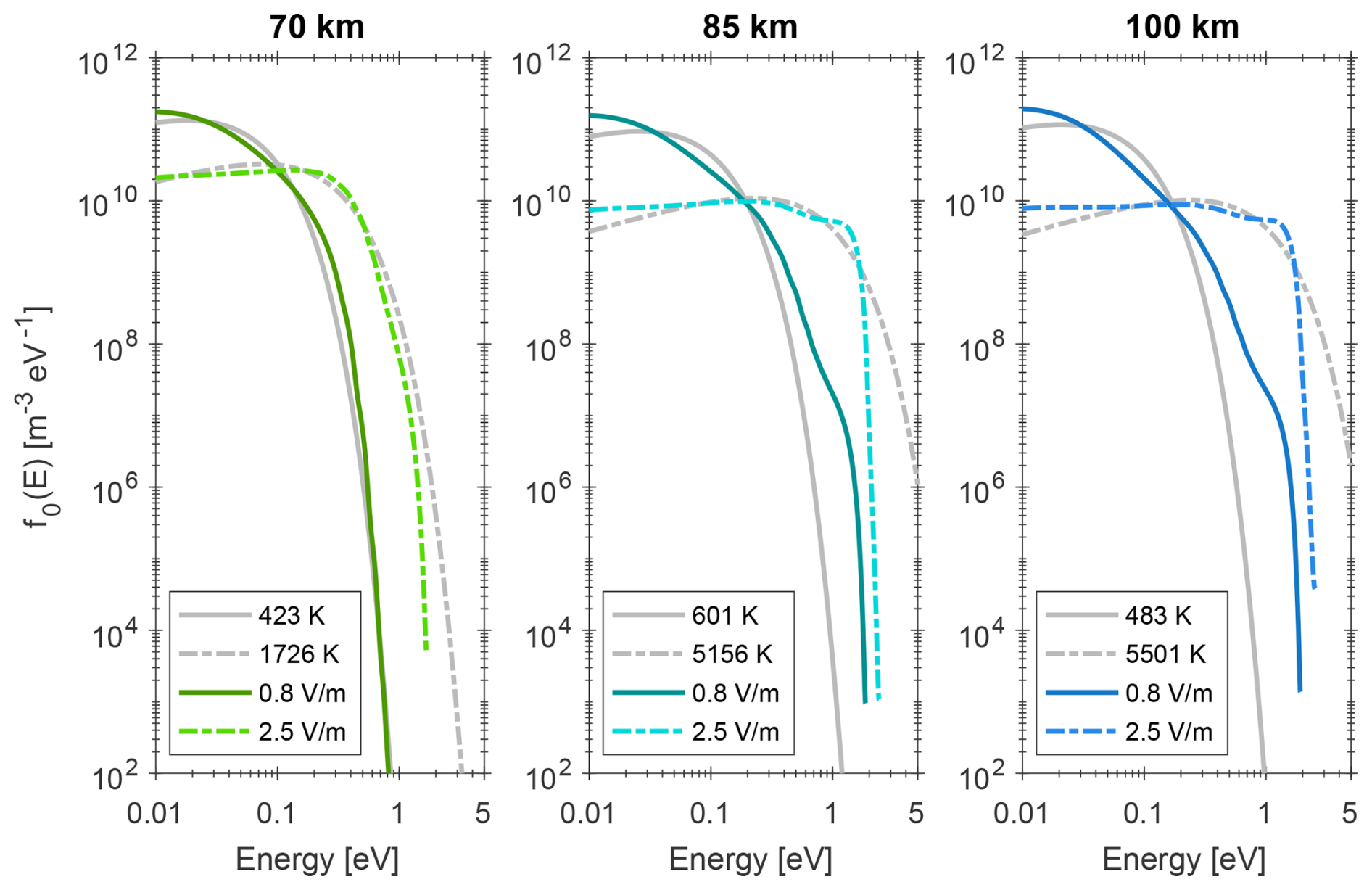
Figure 2 Non-Maxwellian energy distributions (coloured curves) from Eq. (16) at 70, 85 and 100 km, electric fields 0.8 and 2.5 V m⁻¹, and frequency 4.6 MHz. Maxwellian energy distributions (grey curves) at the non-Maxwellian second moment temperature T_2nd. The solid or dashed-dotted curves represents the non-Maxwellian and its corresponding Maxwellian at T_2nd.

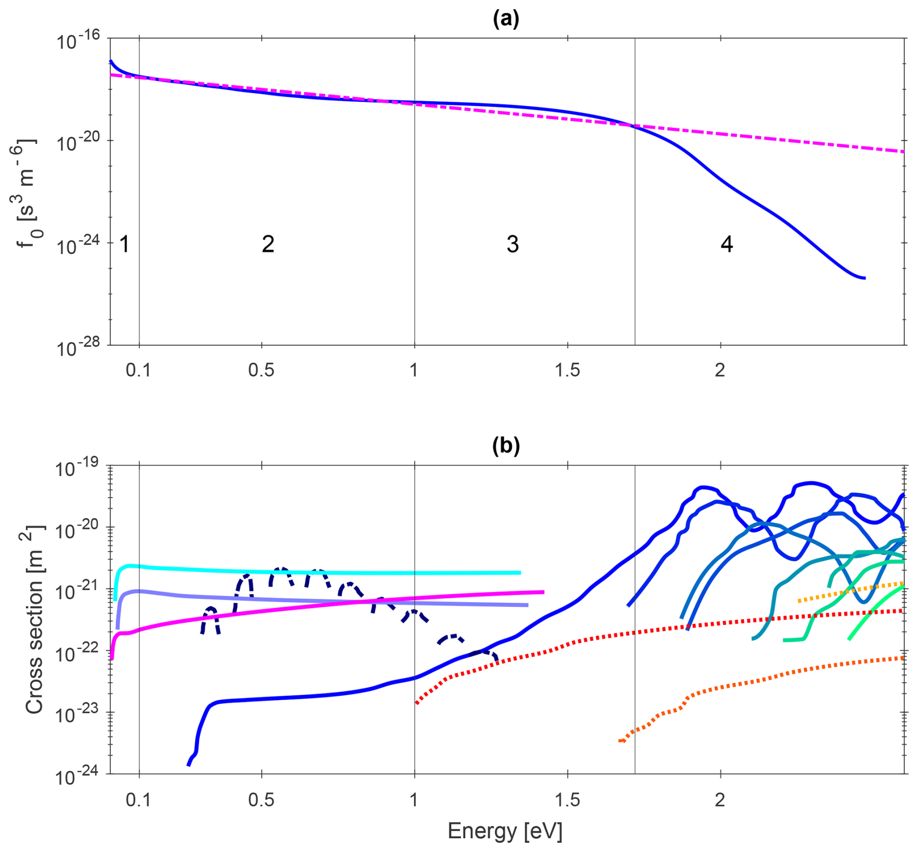
Figure 3 Panel (a): Non-Maxwellian distribution (blue solid curve) at 90 km, electric field 2.0 V m⁻¹ and frequency 4.6 MHz, and Maxwellian distribution (magenta dashed curve) at 5124 K, which is the second moment temperature T_2nd. Panel (b): Inelastic cross sections, which are the same as in Fig. A1. The black vertical lines in both panels marks different energy regions: 1: below 0.1 eV, 2: 0.1–1.0 eV, 3: 1.0–1.8 eV and 4: above 1.8 eV.

5 Results

5.1 Electron distribution

Non-Maxwellian and Maxwellian energy distributions at three altitudes and for two electric field amplitudes are compared in Fig. 2. The temperature of the Maxwellian is taken to be T_2nd (Eq. 20) of the corresponding non-Maxwellian distributions. All the non-Maxwellian distributions in Fig. 2 share some common features, primarily the sharp reduction in phase space density at approximately 2 eV, creating an effective cut-off. This cut-off is caused by the excitation of vibrational states in N₂ with an energy loss of approximately 0.2888 eV per vibrational level. The non-Maxwellian distributions at 70 km appear more Maxwellian, especially for the smaller electric field of 0.8 V m⁻¹. However, with an electric field of 2.5 V m⁻¹ the cut-off become apparent. At 70 km, the neutral density is higher, and all the cooling processes are more effective due to the higher electron-neutral collision frequency. This, in turn, leads to a lower temperature at steady state, even for high electric fields. For electron distributions that are only moderately heated, the deviations from a Maxwellian are less pronounced. The distributions at 85 and 100 km of altitude, which contain more thermal energy, deviates quite significantly from a Maxwellian distribution for both electrical fields. To explain the deviation from a Maxwellian, Fig. 3a shows a non-Maxwellian distribution at 90 km with T_2nd of 5124 K, together with a Maxwellian distribution at the same temperature. Figure 3b shows inelastic cross sections. The vertical black lines in both panels separate four energy regions. By comparing the cross sections to the non-Maxwellian distribution, the deviations from a Maxwellian distribution for the different energy regions can be explained as follows:

• 1.

  Below 0.1 eV: The second term in the numerator (“collision term”) of Eq. (16) is small but non-zero due to excitation of fine structure levels in O and a small contribution from vibrational excitation of N₂ 0-1. In this energy region, the term m_ev is larger than the collision term. The second term in the denominator (“heating term”) is small but still dominates over the collision term. Consequently, the distribution is higher than the Maxwellian at 5124 K. For very small energies close to 0 eV, both the collision term and heating term are zero, while the m_ev and k_bT_n terms are non-zero. As a result, the distribution approximately follows a Maxwellian distribution at the temperature of the neutral gas.

• 2.

  0.1–1.0 eV: Both the excitation of fine structure levels in O and vibrational excitation of O₂ are non-zero. The vibrational excitation of O₂ exhibits resonance peaks in this region, causing electrons to degrade to lower energies by the excitation energy. Here, the collision term is gaining in weight, and as a consequence, the distribution decreases and becomes lower than the Maxwellian.

• 3.

  1.0–1.8 eV: The cross sections for excitation of fine structure levels of O and the vibrational excitation of O₂ decreases, while the vibrational excitation of N₂ and electronic excitation of O₂ remain low. Electrons with energies higher than 2.0 eV degrade to this energy range due to vibrational excitation of N₂. This causes the distribution to fall of more slowly than a Maxwellian.

• 4.

  1.8–2.7 eV: In this energy range, the cross sections for vibrational excitation of N₂ are large, resulting in a significant fraction of electrons exciting vibrational states in N₂ and losing energy. Therefore, the distribution decreases sharply, effectively leading to a cut-off.

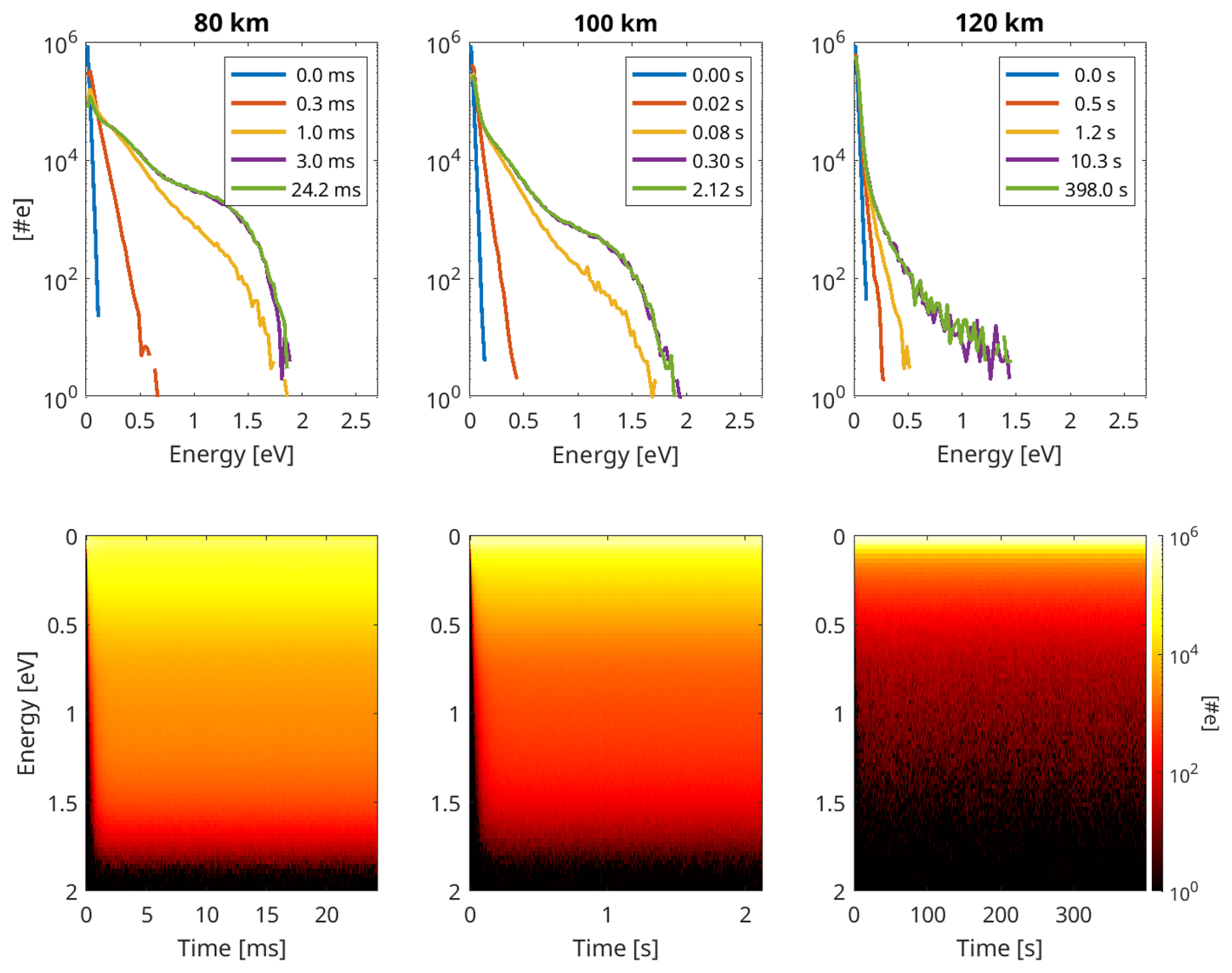
Figure 4 Monte Carlo simulation with an electric field of 1.40 V m⁻¹ at 80 km, 1.12 V m⁻¹ at 100 km and 0.93 V m⁻¹ at 120 km, and frequency 4.6 MHz. First row: Number of electrons per energy bin for different time steps from 0 s to steady state, where steady state is reached at around 3 ms for 80 km, 0.3 s for 100 km and 10 s for 120 km. Second row: Energy of the electrons as a function of time.

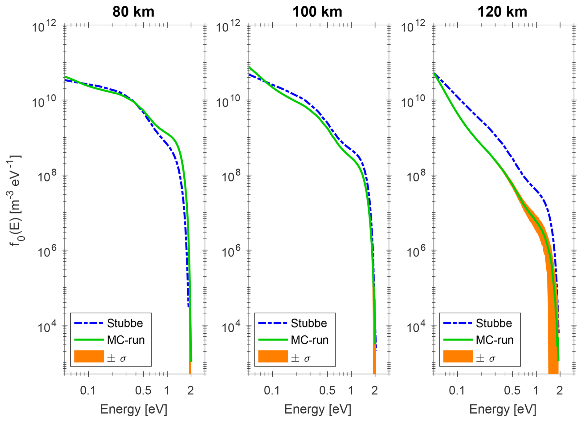
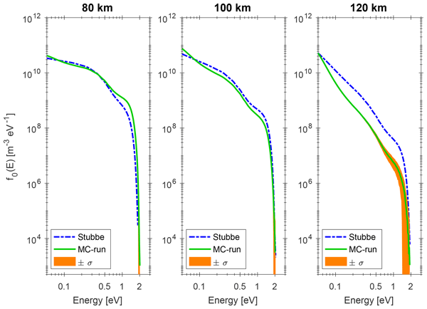
Figure 5 Energy distributions at 80, 100 and 120 km comparing the Monte Carlo simulations to the numerical solution of Boltzmann equation from Eq. (16). The frequency and electric field is the same as Fig. 4. The standard deviation for the Monte Carlo simulation is marked as orange. The electron temperature T_2nd is 1752 K at 80 km, 1232 K at 100 km and 350 K at 120 km for the Boltzmann solver, while for the Monte Carlo simulation T_2nd is 2129 K at 80 km, 934 K at 100 km and 219 K at 120 km.

Figure 4 shows a run of the Monte Carlo simulations at 80, 100 and 120 km. The first row shows the number of electrons per energy bin for different time steps, while the second row shows the energy of the electrons as a function of time. The radio wave has a frequency of 4.6 MHz and an effective radiated power (ERP) of 200 MW. To compute the electric field amplitudes at height z, we use a simplified version of Eq. (16) from Shoucri et al. (1984), given by:

$$\begin{array}{}\text{(22)}& \left|E\right(z\left)\right|=\mathrm{0.25}{\displaystyle \frac{(\mathit{\beta }\cdot W\cdot G{)}^{\mathrm{1}/\mathrm{2}}}{D}}\end{array}$$

where β is the reduction due to absorption at low altitude, assuming no loss in the D region so that β=1, W is the average radiated power, G is the gain of the antenna, and D is the altitude from the ground. Here W⋅G is the ERP. In principle, the actual electric field will depend on the electron density at lower altitudes, which determines how much of the Poynting flux has been absorbed. Here, we choose a representative electric field amplitude to be able to compare the shape of the phase space density for the Monte Carlo simulation and the solution based on Boltzmann equation, and to be able to compare the response at different altitudes. Using Eq. (22) results in an electric field amplitude of 1.40 V m⁻¹ at 80 km, 1.12 V m⁻¹ at 100 km and 0.93 V m⁻¹ at 120 km. The initial time step at 0 s represents a Maxwellian distribution at 300 K. Subsequently, the electrons are accelerated by the HF radio wave. Due to collisions with neutrals, the electrons absorb some energy from the wave, increasing the thermal energy of the electron gas and hence the temperature. At a time step of 0.3 ms for 80 km, 0.02 s for 100 km and 0.5 s for 120 km, the temperature begins to increase. By 1.0 ms for 80 km, 0.08 s for 100 km and 1.2 s for 120 km, the distribution approaches a steady state. After approximately 3.0 ms for 80 km, 0.3 s for 100 km and 10.0 s for 120 km, the distribution effectively reaches a steady state, as the same amount of heat is added by the radio wave and lost through inelastic collisions with neutrals. As shown in the second row of Fig. 4, once electron distribution reaches a steady state, it remains constant over time as long as the heating wave continues to supply energy. The counting statistics of the Monte Carlo simulation at 80 and 100 km are relatively good. However, at energies above approximately 1.8 eV, the number of electrons is small, leading to random fluctuations and a higher standard deviation for the phase space density, as shown in Fig. 5. For 120 km, the spread is much wider even at lower energies, with a significantly higher standard deviation compared to 80 and 100 km, due to the temperature being lower. In addition, the Monte Carlo simulation also allowed us to verify that the phase space density is isotropic to a good degree of accuracy.

Figure 5 presents a comparison between the solution of the Boltzmann equation and the Monte Carlo simulation at 80, 100 and 120 km, using the same frequency and electric field as Fig. 4. At 80 and 100 km, there is a reasonably good agreement between the Monte Carlo simulation and the solution of Boltzmann equation for energies above 0.1 eV. However, the two models differs for energies below 0.1 eV, with the discrepancy decreasing with altitude. This difference might be due to the solution of Boltzmann equation using approximate expressions for rotational excitation and elastic collisions, whereas the Monte Carlo Simulation employs accurate cross sections. Rotational excitation and elastic collisions are more significant at lower altitude due to higher neutral density, which explains why the difference decreases with increasing altitude. At 120 km, the Monte Carlo simulation shows a lower temperature of 219 K compared to 350 K for the Boltzmann solver. This discrepancy arises because electrons gain less energy from the HF radio wave at this altitude, as the electron neutral collision frequency is lower than the gyro-frequency. This violates the assumption in the Boltzmann solution that our electrons are unmagnetized, while the Monte Carlo simulation accounts for the magnetic field. However, the electron-neutral collision frequency becomes slightly lower than the gyro-frequency already at 100 km, where the Boltzmann solver begins to overestimate to some extent. When the electron-neutral collision frequency becomes much lower than the gyro-frequency at 120 km, it becomes evident that the Boltzmann solver overestimates significantly.

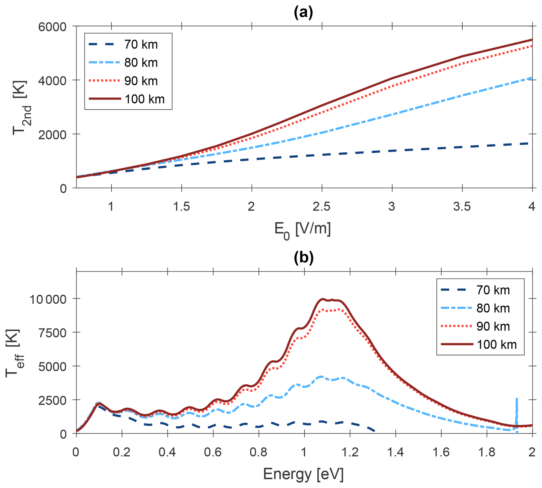
Figure 6 Panel (a): Electron temperature T_2nd, the second moment of the non-Maxwellian distribution, as a function of electric field E₀ at 70–100 km. Panel (b): Electron temperature T_eff as function of energy at 70, 80, 90 and 100 km and electric field 2.0 V m⁻¹.

5.2 Electron temperature

Figure 6a presents T_2nd from Eq. (20) for different heights and electric fields. It is apparent that T_2nd increases with the electric field, i.e. the energy input into the electron gas. However, the temperature increase varies with altitude. For the lowest altitude at 70 km, T_2nd increases from around 400 K with E₀ = 0.75 V m⁻¹ to 1600 K with E₀ = 4.0 V m⁻¹. Meanwhile, at 90–100 km, T_2nd increases from 200–400 K with E₀ = 0.75 V m⁻¹ to 5000–6000 K with E₀ = 4.0 V m⁻¹. The lower heating rates at 70 km can be explained by the very high electron-neutral collision frequency, which causes electrons to collide before they gain much energy from the HF radio wave, thereby reducing the electron heating rate (Kero et al., 2000). In addition, the very high neutral density at this altitude leads to larger cooling rates. At 80–100 km, the electron temperatures are higher because the collision frequency is low enough for electrons to pick up energy between collisions. Furthermore, the lower neutral density at these altitudes reduces the electron cooling rates.

The effective temperature, T_eff (Eq. 21), for an electric field of 2.0 V m⁻¹ at 70, 80, 90 and 100 km is presented in Fig. 6b. T_eff of the non-Maxwellian varies significantly with energy. This variation can be understood by examining T_eff at 90 km, along with the phase space density and cross sections shown in Fig. 3. In the energy range between 1.8 and 2.7 eV, where the cross sections for vibrational excitation of N₂ are large, the temperature is low because a large number of electrons collide with N₂, losing energy and degrading to lower energies. Consequently, the phase density decreases sharply. These electrons degrade to the energy range below 1.8 eV, where the phase space density is relatively flat, causing T_eff to become really high, reaching a peak of around 10 000 K at approximately 1.1 eV. The temperature undulation between 0.1 and 1.2 eV are caused by resonance peaks in the cross sections of vibrational excitation of O₂. The peak at around 0.1 eV is also attributed to the vibrational excitation of O₂, which causes many electrons to degrade down to this energy. At the lowest energies, T_eff approaches to the neutral temperature.

6 Discussion

In this paper, we show that the electron distribution at D region height deviates significantly from a simple Maxwellian, especially when the electrons are heated, by for example high power HF radio waves. The energy variations of the vibrational cross sections of N₂ and O₂ are the main cause of these deviations. While the characteristic shape of Maxwellian distributions remains the same as the temperature increases, the shape of the non-Maxwellian distribution presented in this paper varies with altitude and the energy input to the electron gas. A larger energy input leads to more pronounced deviations. The most eye-catching feature of the distribution is the cut-off at approximately 2 eV, which effectively truncates the distribution. This feature becomes prominent when enough heat is added to the electron gas, allowing a high enough number of electrons to reach energies of 2 eV and above, subsequently exciting vibrational states in N₂. At lower energies, other inelastic collisions, primarily vibrational excitation of O₂, causes additional deviations.

The shape of the Maxwellian is uniquely determined by a single temperature. For a non Maxwellian, it is possible to calculate the second moment, which provides a measure of the thermal energy of the electron gas. However, this second moment does not uniquely determine the shape of the non-Maxwellian distribution since the energy variation of the distribution is not uniform at all heights. A more detailed temperature measure is T_eff (Eq. 21), as defined by Gurevich et al. (1985). For the non-Maxwellian, this temperature varies significantly with energy. On the other hand, for a Maxwellian, T_eff is constant and identical to the standard temperature. These points demonstrate that the standard Maxwellian temperature is not sufficient to describe non-Maxwellian distributions. Furthermore, it is not appropriate to use macroscopic properties, such as cooling rates, calculated from Maxwellian distributions to describe the macroscopic properties of the non-Maxwellian distributions. In the accompanying Part 2, we calculate electron cooling rates for the non-Maxwellian distribution.

These results have been obtained using a solver for the Boltzmann equation, re-implemented from Stubbe (1981) with updated collision cross sections. This version of Boltzmann solver assumes that the electron collision frequency is much higher than the gyro-frequency. While this assumption is valid in the D region, the method must be updated to be applicable for E and F region altitudes, where the electrons are magnetized. To validate the calculated distributions, we compare them with results from a Monte Carlo simulation that integrates the full momentum equation between collisions. In addition to incorporating the effects of the magnetic field, a never ending maintenance task for tools like this is the need to continuously update cross sections.

7 Summary

This work presents non-Maxwellian distributions calculated using a re-implemented numerical Boltzmann equation solver based on Stubbe (1981) with accurate cross sections for inelastic collisions between electrons and neutrals, and an accurate handling of electron energy degradation from higher to lower energies during inelastic collisions. The electron distribution at D region height deviates significantly from a Maxwellian distribution when heated to temperatures exceeding 500–600 K. To quantify the thermal energy of the non-Maxwellian distribution, we use a second moment temperature. However, we demonstrate that no single temperature is sufficient to fully describe these non-Maxwellian distribution.

Appendix A: Cross sections for elastic and inelastic collisions

The cross sections for collisions between electrons and neutrals used in this paper are shown in Fig. A1. These include vibrational excitation of N₂ and O₂, excitation of fine structure levels in O and excitation of electronic levels in O₂ and O. For the excitation of N₂ from the vibrational ground state to levels 1 to 8 in the resonance region 1.5.-5 eV, we use data from Fig. 1 in Campbell et al. (2004). For excitation of the 1. vibrational level from the ground state, we use data from Fig. 2 in Campbell et al. (2004) for the low energy tail region 0.5–1.5 eV and data from Fig. 6.1 in Itikawa et al. (1986) for the high energy tail region 5–100 eV. Cross sections for the vibrational excitation of O₂ are taken from Fig. 6.1 in Itikawa et al. (1989) for the excitation of the vibrational ground state to level 1 in the low energy region below 3 eV, and for higher energies we use a sum of excitation from the ground state to higher levels. For the excitation of fine structure levels in O from the ground state e+O(³P₂) to level 0 and 1, we use data from Fig. 5.1 in Itikawa and Ichimura (1990). For electronic excitation of O₂, we use Fig. 7.2 for the excitation of O₂(a¹Δ_g) and Fig. 7.3 for excitation of ${\mathrm{O}}_{\mathrm{2}}\left(b^{\mathrm{1}}{\sum }_{\mathrm{g}}^{+}\right)$, both from Itikawa et al. (1989). Cross sections for electronic excitation of $\mathrm{O}{(}^{\mathrm{3}}P)\to \mathrm{O}{(}^{\mathrm{1}}S{,}^{\mathrm{1}}D)$ are taken from Fig. 5.2 in Itikawa and Ichimura (1990).

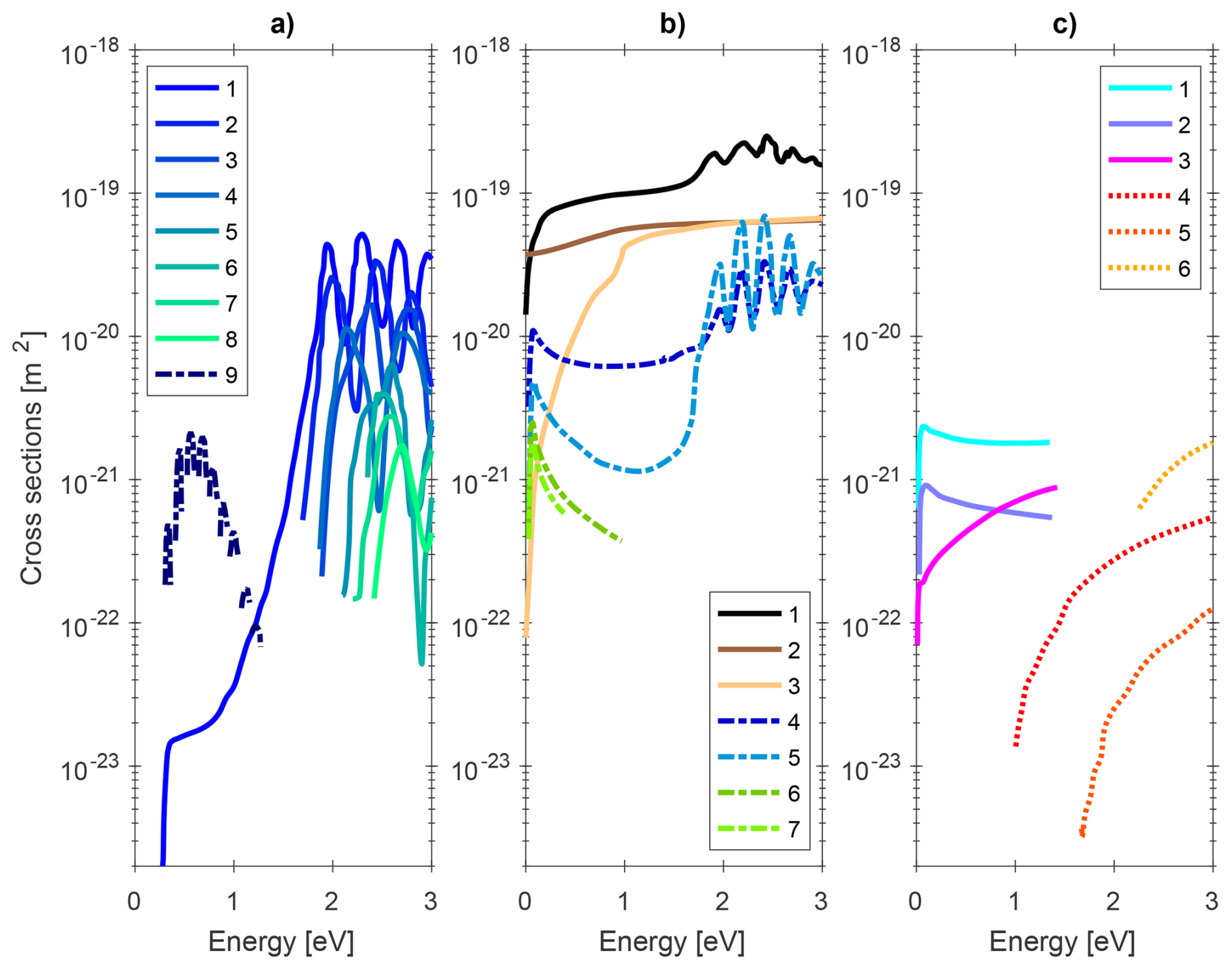
Figure A1 Cross sections for collisions between electrons and neutrals: N₂, O₂ and O. Panel (a) show vibrational cross sections: 1–8. vibrational excitation 0-8 (N₂) and 9. vibrational excitation 0-1 (O₂). Panel (b) show elastic and rotational cross section: 1. elastic (N₂), 2. elastic (O₂), 3. elastic (O) and 4-7. rotational excitation 0-2, 0-4, 0-6 and 0-8 (N₂). Panel (c) show fine structure and electronic cross sections: 1–3. Fine structure excitation of O(³P₂) for 2-1, 2-0 and 1-0, 4. O₂(a¹Δ_g), 5. ${\mathrm{O}}_{\mathrm{2}}\left(b^{\mathrm{1}}{\mathrm{\Sigma }}_{\mathrm{g}}^{+}\right)$ and 6. O(¹D).

In the Monte Carlo simulation, we use the same inelastic cross sections. Additionally, we incorporate cross sections for elastic collisions and rotational excitation of N₂. Cross sections for elastic collisions with N₂ are taken from Fig. 4.2 for energies in the resonance region 1–4 eV and from Fig. 4.1 for energies outside the resonance region; both figures are taken from Itikawa et al. (1986). Furthermore, cross sections for elastic collision with O₂ are taken from Fig. 4.2 in Itikawa et al. (1989), while cross sections for elastic collisions with O are taken from Fig. 4.1 in Itikawa and Ichimura (1990). For the rotational excitation of N₂ (level $\mathrm{0}\to \mathrm{2},\mathrm{4}$), we use data from Fig. 5.2 in Itikawa et al. (1986) for the resonance region 1.4–3 eV. Cross sections outside the resonance region are taken from from Fig. 5.1 in Itikawa et al. (1986) for the excitation of level 0→2 (Born approximation) and for excitation of level $\mathrm{0}\to \mathrm{4},\mathrm{6},\mathrm{8}$ (Onda, 1985).

Appendix B: Derivation of the electron distribution from kinetic theory

The derivation begins with Boltzmann equation:

$$\begin{array}{}\text{(B1)}& \begin{array}{rl}{\displaystyle \frac{\partial }{\partial t}}f(\mathit{r},\mathit{v},t)& +(\mathit{v}\cdot {\mathbf{\nabla }}_{\mathit{r}})f(\mathit{r},\mathit{v},t)\\ & +\left[{\displaystyle \frac{\mathit{F}}{m}}\cdot {\mathbf{\nabla }}_{\mathit{v}}\right]f(\mathit{r},\mathit{v},t)={\left({\displaystyle \frac{\partial f}{\partial t}}\right)}_{\text{coll}}\end{array}\end{array}$$

where $f(\mathit{r},\mathit{v},t)$ is the phase space density, varying in time due to the non-zero velocity of the electrons, external forces acting on the electrons and due to collisions between electrons, neutrals and ions. For external forces we assume that an artificial heating radio wave with an oscillating electric field acts on the electrons:

$$\begin{array}{}\text{(B2)}& \mathit{E}=E_{\mathrm{0}}{\mathit{e}}_{\mathit{x}}\cos \left(\mathit{\omega }t\right)\end{array}$$

Here E₀ is the amplitude of the electric field and ω is the angular frequency of the artificial heating radio wave. For the D region we can assume a cold, weakly ionized, homogenous plasma. Since the neutral density is significantly higher in the D region, electron-neutral collisions dominate over electron-electron and electron-ion collisions, therefore we can neglect the effects of electron-electron and electron-ion collision. In addition, we neglect the influence of Earth's magnetic field since the electron-neutral collision frequency is much higher than the electron gyro-frequency, which means that the electrons are unlikely to complete a gyro-orbit between collisions. With our assumptions for the D region, the Boltzmann equation simplifies to:

$$\begin{array}{}\text{(B3)}& {\displaystyle \frac{\partial f}{\partial t}}+\mathit{\gamma }\cos \left(\mathit{\omega }t\right){\displaystyle \frac{\partial f}{\partial v_x}}={\left({\displaystyle \frac{\partial f}{\partial t}}\right)}_{\text{el}}+{\left({\displaystyle \frac{\partial f}{\partial t}}\right)}_{\text{ie}}\end{array}$$

where f(v,t) is the distribution function in velocity space and γ is the electron acceleration by the heating wave:

$$\begin{array}{}\text{(B4)}& \mathit{\gamma }={\displaystyle \frac{-q_{\mathrm{e}}{E}_{\mathrm{0}}}{m_{\mathrm{e}}}}\end{array}$$

with −q_e as the elementary charge of an electron and m_e as the electron mass. Note that we have neglected the convection term $(\mathit{v}\cdot {\mathbf{\nabla }}_{\mathit{r}})f(\mathit{r},\mathit{v},t)$ since the high collision frequency in the D region gives us a short mean free path l_mfp such that:

$$\begin{array}{}\text{(B5)}& \left|{\displaystyle \frac{\mathrm{\nabla }f\cdot l_{\text{mfp}}}{f}}\right|\ll \mathrm{1}\end{array}$$

and therefore the phase space density evolution will be dominated by local effects. In addition, since E⟂k_HF and the heated beam pattern is wide, the ionosphere appears horizontally smooth.

It is possible to solve f(v,t) by expansion in spherical harmonics with Legendre polynomials and Fourier series (Mintzer, 1964), keeping the first two terms f₀(v) and $f_{\mathrm{1}}(v_x,v,t)$ in the expansion, which leads to:

$$\begin{array}{}\text{(B6)}& \begin{array}{rl}f(\mathit{v},t)& =f_{\mathrm{0}}\left(v\right)+f_{\mathrm{1}}(v_x,v,t)\\ & =f_{\mathrm{0}}\left(v\right)+\mathit{\gamma }{v}_x\left[g_{\mathrm{1}}\right(v\left)\cos \right(\mathit{\omega }t)+h_{\mathrm{1}}(v\left)\sin \right(\mathit{\omega }t\left)\right]\end{array}\end{array}$$

where f₀(v) is the symmetric part of the distribution function and $f_{\mathrm{1}}(v_x,v,t)$ is the asymmetric part of the distribution function (the perturbation term). It is worthwhile to note that f₀, g₁ and h₁ only depends upon the magnitude of $v=\left|\mathit{v}\right|$, as stated in Mintzer (1964) and in Milikh and Dimant (2003), because the distribution is close to being spherically symmetric as a result of repeated elastic collisions. Furthermore, Stubbe (1981) makes the simplifying assumption that:

$$\begin{array}{}\text{(B7)}& \begin{array}{rl}& {\left({\displaystyle \frac{\partial f}{\partial t}}\right)}_{\text{el}}+{\left({\displaystyle \frac{\partial f}{\partial t}}\right)}_{\text{ie}}\\ & \textcolor{red}{}\end{array}\end{array}$$

since f₀ is almost perfectly isotropic and elastic collisions only change the direction of the electron velocity, it follows that $(\partial f_{\mathrm{0}}/\partial t{)}_{\text{el}}=\mathrm{0}$. Furthermore, since elastic cross section are larger than inelastic cross sections, $(\partial f_{\mathrm{1}}/\partial t{)}_{\text{ie}}$ can be neglected.

To get a expression for the elastic collision integral, Stubbe (1981) uses the Lorentz approximation. The Lorentz approximation is based on the assumption that since m_e≪M, where m_e is the mass of the electron and M is the mass of the neutral, the electron velocity is much higher than the velocity of neutrals. The relative velocity between electrons and neutrals can then be replaced with the electron velocity. In addition, it is assumed that the electron and neutral velocity will remain the same before and after collision with no energy exchange between electrons and neutrals. The starting point for the derivation is the Boltzmann collision integral for elastic collisions from Mintzer (1964):

$$\begin{array}{}\text{(B8)}& \begin{array}{rl}{\left({\displaystyle \frac{\partial f_{\mathrm{1}}}{\partial t}}\right)}_{\text{el}}=& -\int \left[f\left(\mathit{v}\right)F\left(\mathit{V}\right)-f\left({\mathit{v}}^{\prime }\right)F\left({\mathit{V}}^{\prime }\right)\right]\\ & \times g\stackrel{\mathrm{̃}}{b}\mathrm{d}\stackrel{\mathrm{̃}}{b}\mathrm{d}\mathit{ϵ}\mathrm{d}\mathit{V}\end{array}\end{array}$$

where F(V) is a Maxwellian distribution function for the neutrals, and un-primed velocities are before collision and primed velocities are after collision. Moreover, the parameter $\stackrel{\mathrm{̃}}{b}$ is the impact parameter, g is the relative velocity between electrons and neutrals, and ϵ is an angle that takes into account collisions for all directions. Differentiating f₁ from Eq. B6 with regard to time gives for the elastic collision integral:

$$\begin{array}{}\text{(B9)}& {\left({\displaystyle \frac{\partial f_{\mathrm{1}}}{\partial t}}\right)}_{\text{el}}=\mathit{\gamma }\cos \mathit{\omega }t\left({\displaystyle \frac{\partial v_x{g}_{\mathrm{1}}}{\partial t}}\right)+\mathit{\gamma }\sin \mathit{\omega }t\left({\displaystyle \frac{\partial v_x{h}_{\mathrm{1}}}{\partial t}}\right)\end{array}$$

for the perturbation terms v_xg₁ and v_xh₁. Inserting the perturbation terms in Eq. (B8) and applying the Lorentz approximation gives:

$$\begin{array}{}\text{(B10)}& \begin{array}{rl}& \left({\displaystyle \frac{\partial v_x{h}_{\mathrm{1}}}{\partial t}}\right)=-h_{\mathrm{1}}\left(v\right)v_x\mathit{\nu }\left(v\right)\\ & \left({\displaystyle \frac{\partial v_x{g}_{\mathrm{1}}}{\partial t}}\right)=-g_{\mathrm{1}}\left(v\right)v_x\mathit{\nu }\left(v\right)\end{array}\end{array}$$

with the electron-neutral collision frequency for momentum transfer given by:

$$\begin{array}{}\text{(B11)}& \mathit{\nu }\left(v\right)=\mathrm{2}\mathit{\pi }{N}_{\mathrm{n}}v\underset{\mathrm{0}}{\overset{\mathrm{\infty }}{\int }}[\mathrm{1}-cos\mathit{\theta }(v,\stackrel{\mathrm{̃}}{b}\left)\right]\stackrel{\mathrm{̃}}{b}d\stackrel{\mathrm{̃}}{b}\end{array}$$

where $N_{\mathrm{n}}={\mathrm{N}}_{\mathrm{2}}+{\mathrm{O}}_{\mathrm{2}}+\mathrm{O}$ is the neutral density and N₂ and O₂ are the number density of N₂ or O₂, respectively, and O is the number density of O. Finally, by putting Eq. (B10) in Eq. (B9) we get:

$$\begin{array}{}\text{(B12)}& \begin{array}{rl}{\left({\displaystyle \frac{\partial f_{\mathrm{1}}}{\partial t}}\right)}_{\text{el}}=& -\mathit{\gamma }{v}_x\mathit{\nu }\left(v\right)\left[g_{\mathrm{1}}\right(v\left)\cos \right(\mathit{\omega }t)\\ & +h_{\mathrm{1}}\left(v\right)\sin \left(\mathit{\omega }t\right)]\end{array}\end{array}$$

As in Stubbe (1981), we use an approximate expression from Phelps and Pack (1959) and Hake and Phelps (1967) for the electron-neutral collision frequency ν(v) instead of Eq. (B11):

$$\begin{array}{}\text{(B13)}& \mathit{\nu }\left(v\right)=b{N}_{\mathrm{n}}{v}^{\mathrm{2}}\end{array}$$

where b = 2.8 × 10⁻²³ cm s⁻¹.

The inelastic collision integral consists of several parts: rotational excitation, vibrational excitation, electron excitation and excitation of fine structure levels in atomic oxygen. For excitation (disregarding de-excitation) the general form of the inelastic collision integral is given by (Gurevich, 1978; Holstein, 1946):

$$\begin{array}{}\text{(B14)}& {\displaystyle }\begin{array}{rl}& {\left({\displaystyle \frac{\partial f_{\mathrm{0}}}{\partial t}}\right)}_{\text{ie}}\\ =& -\underset{\text{loss\hspace{0.17em}\hspace{0.17em}of\hspace{0.17em}\hspace{0.17em}phase\hspace{0.17em}\hspace{0.17em}space\hspace{0.17em}\hspace{0.17em}density\hspace{0.17em}\hspace{0.17em}from\hspace{0.17em}\hspace{0.17em}energy\hspace{0.17em} }E}{\underbrace{\sum _l\sum _{k=\mathrm{0}}^{M-\mathrm{1}}\sum _{j=k+\mathrm{1}}^M{N}_l^k{\displaystyle \frac{\mathrm{2}}{m_{\mathrm{e}}v\left(E\right)}}E{f}_{\mathrm{0}}\left(E\right){\mathit{\sigma }}_l^{k\to j}\left(E\right)}}\end{array}\text{(B15)}& {\displaystyle }+\underset{\begin{array}{c}\text{contribution\hspace{0.17em}\hspace{0.17em}to\hspace{0.17em}\hspace{0.17em}phase\hspace{0.17em}\hspace{0.17em}space\hspace{0.17em}\hspace{0.17em}density\hspace{0.17em}\hspace{0.17em}at\hspace{0.17em} }E\\ \text{from\hspace{0.17em}\hspace{0.17em}higher\hspace{0.17em}\hspace{0.17em}energies}\end{array}}{\underbrace{\begin{array}{c}\sum _l\sum _{k=\mathrm{0}}^{M-\mathrm{1}}\sum _{j=k+\mathrm{1}}^M{N}_l^k\frac{\mathrm{2}}{m_{\mathrm{e}}v(E+\mathrm{\Delta }{E}_l^{k\to j})}\\ \times \left(E+\mathrm{\Delta }{E}_l^{k\to j}\right)f_{\mathrm{0}}\left(E+\mathrm{\Delta }{E}_l^{k\to j}\right){\mathit{\sigma }}_l^{k\to j}\\ \times (E+E_k^j)\end{array}}}\end{array}$$

where the neutral constituent $N_l^k$ is excited from energy state k→j, M is the total number of energy states, $E=\frac{\mathrm{1}}{\mathrm{2}}{m}_{\mathrm{e}}{v}^{\mathrm{2}}$ is the electron energy, $\mathrm{\Delta }{E}_l^{k\to j}$ is the excitation energy and ${\mathit{\sigma }}_l^{k\to j}$ is the cross section. Rotational excitation can be simplified (Gurevich, 1978) because $\mathrm{\Delta }{E}_l^{k\to j}\ll E$:

$$\begin{array}{}\text{(B16)}& {\left({\displaystyle \frac{\partial f_{\mathrm{0}}}{\partial t}}\right)}_{\text{rot}}={\displaystyle \frac{\mathrm{4}{\mathit{\sigma }}_{\mathrm{0}}{B}_{\mathrm{0}}}{m_{\mathrm{e}}}}{N}_{\mathrm{n}\mathrm{2}}{\displaystyle \frac{\mathrm{1}}{v^{\mathrm{2}}}}{\displaystyle \frac{\partial }{\partial v}}\left[{\displaystyle \frac{k_b{T}_{\mathrm{n}}}{m_{\mathrm{e}}}}v{\displaystyle \frac{\partial f_{\mathrm{0}}}{\partial v}}+v^{\mathrm{2}}{f}_{\mathrm{0}}\right]\end{array}$$

where $N_{\mathrm{n}\mathrm{2}}={\mathrm{N}}_{\mathrm{2}}+{\mathrm{O}}_{\mathrm{2}}$. For excitation of vibrational states, electronic states and fine structure levels we only consider excitation from the ground state, which simplifies Eq. (B15) to:

$$\begin{array}{}\text{(B17)}& \begin{array}{rl}{\left({\displaystyle \frac{\partial f_{\mathrm{0}}}{\partial t}}\right)}_{\text{ie}}=& {\displaystyle \frac{\mathrm{2}}{m_{\mathrm{e}}v}}\sum _l{N}_l\sum _{j=\mathrm{1}}^{\mathrm{\infty }}[-E{f}_{\mathrm{0}}(E\left){\mathit{\sigma }}_l^j\right(E)\\ & +\left(E+\mathrm{\Delta }{E}_l^j\right)f_{\mathrm{0}}\left(E+\mathrm{\Delta }{E}_l^j\right)\\ & \times {\mathit{\sigma }}_l^j\left(E+\mathrm{\Delta }{E}_l^j\right)]\end{array}\end{array}$$

where $\mathrm{\Delta }{E}_l^j$ is the excitation energy from ground state to the state j with the cross section ${\mathit{\sigma }}_l^j$ for the different neutral constituents N_l of N₂, O₂ or O in the ground state.

We then proceed to derive an expression for the distribution function f(v,t), starting by differentiating the expression for the distribution given by Eq. (B6), which has been expanded in spherical harmonics. First, we differentiate with regard to time:

$$\begin{array}{}\text{(B18)}& {\displaystyle \frac{\partial f}{\partial t}}={\displaystyle \frac{\partial f_{\mathrm{0}}}{\partial t}}+\mathit{\gamma }{v}_x\mathit{\omega }[-g_{\mathrm{1}}(v\left)\sin \right(\mathit{\omega }t)+h_{\mathrm{1}}(v\left)\cos \right(\mathit{\omega }t\left)\right]\end{array}$$

and then with regard to v_x:

$$\begin{array}{}\text{(B19)}& \begin{array}{rl}{\displaystyle \frac{\partial f}{\partial v_x}}=& {\displaystyle \frac{\partial f_{\mathrm{0}}}{\partial v_x}}+\mathit{\gamma }\left[g_{\mathrm{1}}\right(v\left)\cos \right(\mathit{\omega }t)+h_{\mathrm{1}}(v\left)\sin \right(\mathit{\omega }t\left)\right]\\ & +\mathit{\gamma }{v}_x\left[{\displaystyle \frac{\partial g_{\mathrm{1}}}{\partial v_x}}\cos \left(\mathit{\omega }t\right)+{\displaystyle \frac{\partial h_{\mathrm{1}}}{\partial v_x}}\sin \mathit{\omega }t)\right]\end{array}\end{array}$$

which can be put into Boltzmann Eq. (B3), giving:

$$\begin{array}{}\text{(B20)}& \begin{array}{rl}& \textcolor{red}{}\\ & +\mathit{\gamma }\cos \left(\mathit{\omega }t\right){\displaystyle \frac{\partial f_{\mathrm{0}}}{\partial v_x}}+{\mathit{\gamma }}^{\mathrm{2}}\cos \left(\mathit{\omega }t\right)\left[g_{\mathrm{1}}\right(v\left)\cos \right(\mathit{\omega }t)\\ & +h_{\mathrm{1}}\left(v\right)\sin \left(\mathit{\omega }t\right)]+{\mathit{\gamma }}^{\mathrm{2}}\cos (\mathit{\omega }t)\\ & \times v_x\left[{\displaystyle \frac{\partial g_{\mathrm{1}}}{\partial v_x}}\cos \left(\mathit{\omega }t\right)+{\displaystyle \frac{\partial h_{\mathrm{1}}}{\partial v_x}}\sin \mathit{\omega }t)\right]\\ =& {\left({\displaystyle \frac{\partial f_{\mathrm{1}}}{\partial t}}\right)}_{\text{el}}+{\left({\displaystyle \frac{\partial f_{\mathrm{0}}}{\partial t}}\right)}_{\text{ie}}\end{array}\end{array}$$

The term containing the time derivative of f₀ have been left out because we are only interested in solving for the distribution function for steady state conditions. Then, the coefficient for each frequency component can be equated: the DC-term (ω=0), the heating frequency (ω) and the second harmonic (2ω). We start with ω:

$$\begin{array}{}\text{(B21)}& \begin{array}{rl}& \mathit{\gamma }{v}_x\mathit{\omega }[-g_{\mathrm{1}}(v\left)\sin \right(\mathit{\omega }t)+h_{\mathrm{1}}(v\left)\cos \right(\mathit{\omega }t\left)\right]\\ & +\mathit{\gamma }\cos \left(\mathit{\omega }t\right){\displaystyle \frac{\partial f_{\mathrm{0}}}{\partial v_x}}\\ & =-\mathit{\gamma }{v}_x\mathit{\nu }\left(v\right)\left[g_{\mathrm{1}}\right(v\left)\cos \right(\mathit{\omega }t)+h_{\mathrm{1}}(v\left)\sin \right(\mathit{\omega }t\left)\right]\end{array}\end{array}$$

Note that the right hand side of this equation is the elastic collision integral from Eq. (B12). Terms with γcos (ωt) gives:

$$\begin{array}{}\text{(B22)}& \begin{array}{rl}\mathit{\gamma }{v}_x\mathit{\omega }{h}_{\mathrm{1}}+\mathit{\gamma }{\displaystyle \frac{\partial f_{\mathrm{0}}}{\partial v_x}}& =-\mathit{\gamma }{v}_x\mathit{\nu }{g}_{\mathrm{1}}\Rightarrow g_{\mathrm{1}}\\ & =-{\displaystyle \frac{\mathit{\nu }}{{\mathit{\omega }}^{\mathrm{2}}+{\mathit{\nu }}^{\mathrm{2}}}}{\displaystyle \frac{\mathrm{1}}{v_x}}{\displaystyle \frac{\partial f_{\mathrm{0}}}{\partial v_x}}\end{array}\end{array}$$

while terms with γsin (ωt) gives:

$$\begin{array}{}\text{(B23)}& \begin{array}{rl}-\mathit{\gamma }{v}_x\mathit{\omega }{g}_{\mathrm{1}}& =-\mathit{\gamma }{v}_x\mathit{\nu }{h}_{\mathrm{1}}\Rightarrow h_{\mathrm{1}}={\displaystyle \frac{\mathit{\omega }{g}_{\mathrm{1}}}{\mathit{\nu }}}\\ & =-{\displaystyle \frac{\mathit{\omega }}{{\mathit{\omega }}^{\mathrm{2}}+{\mathit{\nu }}^{\mathrm{2}}}}{\displaystyle \frac{\mathrm{1}}{v_x}}{\displaystyle \frac{\partial f_{\mathrm{0}}}{\partial v_x}}\end{array}\end{array}$$

The DC-term and the second harmonic term results in:

$$\begin{array}{}\text{(B24)}& \begin{array}{rl}& {\mathit{\gamma }}^{\mathrm{2}}\cos \left(\mathit{\omega }t\right)\left[g_{\mathrm{1}}\right(v\left)\cos \right(\mathit{\omega }t)+h_{\mathrm{1}}(v\left)\sin \right(\mathit{\omega }t\left)\right]\\ & +{\mathit{\gamma }}^{\mathrm{2}}\cos \left(\mathit{\omega }t\right)v_x\left[{\displaystyle \frac{\partial g_{\mathrm{1}}}{\partial v_x}}\cos \left(\mathit{\omega }t\right)+{\displaystyle \frac{\partial h_{\mathrm{1}}}{\partial v_x}}\sin \mathit{\omega }t)\right]\\ =& {\left({\displaystyle \frac{\partial f_{\mathrm{0}}}{\partial t}}\right)}_{\text{ie}}\end{array}\end{array}$$

All the terms with h₁ disappear because averaging over a full period of the term cos (ωt)sin (ωt) is equal to zero, and then Eq. B24 leaves:

$$\begin{array}{}\text{(B25)}& {\displaystyle \frac{\mathrm{1}}{\mathrm{2}}}{\mathit{\gamma }}^{\mathrm{2}}\left(g_{\mathrm{1}}+v_x{\displaystyle \frac{\partial g_{\mathrm{1}}}{\partial v_x}}\right)={\left({\displaystyle \frac{\partial f_{\mathrm{0}}}{\partial t}}\right)}_{\text{ie}}\end{array}$$

where the term with g₁ becomes zero (Chapman and Cowling, 1939). Inserting Eq. (B22) into Eq. (B25):

$$\begin{array}{}\text{(B26)}& -{\displaystyle \frac{\mathrm{1}}{\mathrm{2}}}{\mathit{\gamma }}^{\mathrm{2}}{v}_x{\displaystyle \frac{\partial }{\partial v_x}}\left[{\displaystyle \frac{\mathit{\nu }}{{\mathit{\omega }}^{\mathrm{2}}+{\mathit{\nu }}^{\mathrm{2}}}}{\displaystyle \frac{\mathrm{1}}{v_x}}{\displaystyle \frac{\partial f_{\mathrm{0}}}{\partial v_x}}\right]={\left({\displaystyle \frac{\partial f_{\mathrm{0}}}{\partial t}}\right)}_{\text{ie}}\end{array}$$

By using the Laplacian in spherical coordinates:

$$\begin{array}{}\text{(B27)}& {\mathbf{\nabla }}_v^{\mathrm{2}}={\displaystyle \frac{\mathrm{1}}{v^{\mathrm{2}}}}{\displaystyle \frac{\partial }{\partial v}}\left(v^{\mathrm{2}}{\displaystyle \frac{\partial f}{\partial v}}\right)\end{array}$$

neglecting the terms with ϕ and θ since the distribution is assumed to be isotropic and assuming (Mintzer, 1964):

$$\begin{array}{}\text{(B28)}& v_x^{\mathrm{2}}={\displaystyle \frac{v^{\mathrm{2}}}{\mathrm{3}}}\end{array}$$

we get:

$$\begin{array}{}\text{(B29)}& -{\displaystyle \frac{\mathrm{1}}{\mathrm{6}}}{\displaystyle \frac{{\mathit{\gamma }}^{\mathrm{2}}}{v^{\mathrm{2}}}}{\displaystyle \frac{\partial }{\partial v}}\left[{\displaystyle \frac{\mathit{\nu }{v}^{\mathrm{2}}}{{\mathit{\omega }}^{\mathrm{2}}+{\mathit{\nu }}^{\mathrm{2}}}}{\displaystyle \frac{\partial f_{\mathrm{0}}}{\partial v}}\right]={\left({\displaystyle \frac{\partial f_{\mathrm{0}}}{\partial t}}\right)}_{\text{ie}}\end{array}$$

Multiplying Eq. (B29) with 4πv² and $\mathrm{1}/N_{\mathrm{n}\mathrm{2}}$ and integrating from zero to v:

$$\begin{array}{}\text{(B30)}& \begin{array}{rl}& -{\displaystyle \frac{{\mathit{\gamma }}^{\mathrm{2}}}{\mathrm{6}}}{\displaystyle \frac{\mathrm{1}}{N_{\mathrm{n}\mathrm{2}}}}\underset{\mathrm{0}}{\overset{v}{\int }}{\displaystyle \frac{\partial }{\partial v}}\left[{\displaystyle \frac{\mathit{\nu }{v}^{\mathrm{2}}}{{\mathit{\omega }}^{\mathrm{2}}+{\mathit{\nu }}^{\mathrm{2}}}}{\displaystyle \frac{\partial f_{\mathrm{0}}}{\partial v}}\right]\mathrm{d}v\\ =& {\displaystyle \frac{\mathrm{1}}{N_{\mathrm{n}\mathrm{2}}}}\underset{\mathrm{0}}{\overset{v}{\int }}{v}^{\mathrm{2}}{\left({\displaystyle \frac{\partial f_{\mathrm{0}}}{\partial t}}\right)}_{\text{ie}}\mathrm{d}v\end{array}\end{array}$$

and for simplification defining:

$$\begin{array}{}\text{(B31)}& G\left(v\right)={\displaystyle \frac{\mathrm{1}}{N_{\mathrm{n}\mathrm{2}}}}\underset{\mathrm{0}}{\overset{v}{\int }}{v}^{\mathrm{2}}{\left({\displaystyle \frac{\partial f_{\mathrm{0}}}{\partial t}}\right)}_{\text{vib}}\mathrm{d}v\end{array}$$

If we insert expressions for the inelastic collision integral for rotational excitation from Eq. (B16) and ν(v) from Eq. (B13), we obtain:

$$\begin{array}{}\text{(B32)}& \begin{array}{rl}& -{\displaystyle \frac{\mathrm{1}}{\mathrm{6}}}b{\displaystyle \frac{N_{\mathrm{n}}}{N_{\mathrm{n}\mathrm{2}}}}{\mathit{\gamma }}^{\mathrm{2}}\left[{\displaystyle \frac{v^{\mathrm{4}}}{{\mathit{\omega }}^{\mathrm{2}}+{\mathit{\nu }}^{\mathrm{2}}}}{\displaystyle \frac{\partial f_{\mathrm{0}}}{\partial v}}\right]\\ =& {\displaystyle \frac{\mathrm{1}}{N_{\mathrm{n}\mathrm{2}}}}\underset{\mathrm{0}}{\overset{v}{\int }}\left({\displaystyle \frac{\mathrm{4}{\mathit{\sigma }}_{\mathrm{0}}{B}_{\mathrm{0}}{N}_{\mathrm{n}\mathrm{2}}}{m_{\mathrm{e}}}}{\displaystyle \frac{\partial }{\partial v}}\left[{\displaystyle \frac{k_b{T}_{\mathrm{n}}}{m_{\mathrm{e}}}}v{\displaystyle \frac{\partial f_{\mathrm{0}}}{\partial v}}+v^{\mathrm{2}}{f}_{\mathrm{0}}\right]\right)\mathrm{d}v\\ & +G\left(v\right)\end{array}\end{array}$$

and defining $r_{\mathrm{N}}=N_{\mathrm{n}}/N_{\mathrm{n}\mathrm{2}}$. Then, we simplify the equation:

$$\begin{array}{}\text{(B33)}& \begin{array}{rl}& -{\displaystyle \frac{\mathrm{1}}{\mathrm{6}}}b{r}_{\mathrm{N}}{\mathit{\gamma }}^{\mathrm{2}}\left[{\displaystyle \frac{v^{\mathrm{4}}}{{\mathit{\omega }}^{\mathrm{2}}+{\mathit{\nu }}^{\mathrm{2}}}}{\displaystyle \frac{\partial f_{\mathrm{0}}}{\partial v}}\right]\\ & =\left({\displaystyle \frac{\mathrm{4}{\mathit{\sigma }}_{\mathrm{0}}{B}_{\mathrm{0}}}{m_{\mathrm{e}}}}\left[{\displaystyle \frac{k_b{T}_{\mathrm{n}}}{m_{\mathrm{e}}}}v{\displaystyle \frac{\partial f_{\mathrm{0}}}{\partial v}}+v^{\mathrm{2}}{f}_{\mathrm{0}}\right]\right)+G\left(v\right)\end{array}\end{array}$$

and multiply by $m_{\mathrm{e}}^{\mathrm{2}}$ and (4σ₀B₀vf₀)⁻¹:

$$\begin{array}{}\text{(B34)}& \begin{array}{rl}& -{\displaystyle \frac{m_{\mathrm{e}}^{\mathrm{2}}b{r}_{\mathrm{N}}{\mathit{\gamma }}^{\mathrm{2}}}{\mathrm{24}{\mathit{\sigma }}_{\mathrm{0}}{B}_{\mathrm{0}}v}}\left[{\displaystyle \frac{v^{\mathrm{4}}}{{\mathit{\omega }}^{\mathrm{2}}+{\mathit{\nu }}^{\mathrm{2}}}}\right]{\displaystyle \frac{\mathrm{1}}{f_{\mathrm{0}}}}{\displaystyle \frac{\partial f_{\mathrm{0}}}{\partial v}}\\ =& k_b{T}_{\mathrm{n}}{\displaystyle \frac{\mathrm{1}}{f_{\mathrm{0}}}}{\displaystyle \frac{\partial f_{\mathrm{0}}}{\partial v}}+m_{\mathrm{e}}v+{\displaystyle \frac{m_{\mathrm{e}}^{\mathrm{2}}G\left(u\right)}{\mathrm{4}{\mathit{\sigma }}_{\mathrm{0}}{B}_{\mathrm{0}}v{f}_{\mathrm{0}}}}\end{array}\end{array}$$

Rearranging:

$$\begin{array}{}\text{(B35)}& {\displaystyle \frac{\mathrm{1}}{f_{\mathrm{0}}}}{\displaystyle \frac{\partial f_{\mathrm{0}}}{\partial v}}=-\left({\displaystyle \frac{{\displaystyle }{m}_{\mathrm{e}}v+{\displaystyle \frac{m_{\mathrm{e}}^{\mathrm{2}}G\left(v\right)}{\mathrm{4}{\mathit{\sigma }}_{\mathrm{0}}{B}_{\mathrm{0}}v{f}_{\mathrm{0}}}}}{{\displaystyle }{k}_b{T}_{\mathrm{n}}+{\displaystyle \frac{m_{\mathrm{e}}^{\mathrm{2}}b{r}_{\mathrm{N}}{\mathit{\gamma }}^{\mathrm{2}}}{\mathrm{24}{\mathit{\sigma }}_{\mathrm{0}}{B}_{\mathrm{0}}}}{\displaystyle \frac{v^{\mathrm{3}}}{{\mathit{\omega }}^{\mathrm{2}}+{\mathit{\nu }}^{\mathrm{2}}}}}}\right)\end{array}$$

which we can try to treat as a separable differential equation. Integrating both sides:

$$\begin{array}{}\text{(B36)}& \underset{\mathrm{0}}{\overset{v}{\int }}{\displaystyle \frac{\mathrm{1}}{f_{\mathrm{0}}}}\mathrm{d}{f}_{\mathrm{0}}=-\underset{\mathrm{0}}{\overset{v}{\int }}\left({\displaystyle \frac{{\displaystyle }{m}_{\mathrm{e}}v+{\displaystyle \frac{m_{\mathrm{e}}^{\mathrm{2}}G\left(v\right)}{\mathrm{4}{\mathit{\sigma }}_{\mathrm{0}}{B}_{\mathrm{0}}v{f}_{\mathrm{0}}\left(v\right)}}}{{\displaystyle }{k}_b{T}_{\mathrm{n}}+{\displaystyle \frac{m_{\mathrm{e}}^{\mathrm{2}}b{r}_{\mathrm{N}}{\mathit{\gamma }}^{\mathrm{2}}}{\mathrm{24}{\mathit{\sigma }}_{\mathrm{0}}{B}_{\mathrm{0}}}}{\displaystyle \frac{v^{\mathrm{3}}}{{\mathit{\omega }}^{\mathrm{2}}+{\mathit{\nu }}^{\mathrm{2}}}}}}\right)\mathrm{d}v\end{array}$$

gives:

$$\begin{array}{}\text{(B37)}& {\displaystyle \frac{\log f_{\mathrm{0}}\left(v\right)}{\log \underset{\text{A}}{\underbrace{f_{\mathrm{0}}\left(\mathrm{0}\right)}}}}=-\underset{\mathrm{0}}{\overset{v}{\int }}\left({\displaystyle \frac{{\displaystyle }{m}_{\mathrm{e}}v+{\displaystyle \frac{m_{\mathrm{e}}^{\mathrm{2}}G\left(v\right)}{\mathrm{4}{\mathit{\sigma }}_{\mathrm{0}}{B}_{\mathrm{0}}v{f}_{\mathrm{0}}\left(v\right)}}}{{\displaystyle }{k}_b{T}_{\mathrm{n}}+{\displaystyle \frac{m_{\mathrm{e}}^{\mathrm{2}}b{r}_{\mathrm{N}}{\mathit{\gamma }}^{\mathrm{2}}}{\mathrm{24}{\mathit{\sigma }}_{\mathrm{0}}{B}_{\mathrm{0}}}}{\displaystyle \frac{v^{\mathrm{3}}}{{\mathit{\omega }}^{\mathrm{2}}+{\mathit{\nu }}^{\mathrm{2}}}}}}\right)\mathrm{d}v\end{array}$$

and by taking the exponent on both sides finally gives:

$$\begin{array}{}\text{(B38)}& f_{\mathrm{0}}\left(v\right)=A\exp \left\{-{\displaystyle }\underset{\mathrm{0}}{\overset{v}{\int }}{\displaystyle \frac{{\displaystyle }{m}_{\mathrm{e}}v+{\displaystyle \frac{m_{\mathrm{e}}^{\mathrm{2}}G\left(v\right)}{\mathrm{4}{\mathit{\sigma }}_{\mathrm{0}}{B}_{\mathrm{0}}v{f}_{\mathrm{0}}\left(v\right)}}}{{\displaystyle }{k}_b{T}_{\mathrm{n}}+{\displaystyle \frac{m_{\mathrm{e}}^{\mathrm{2}}b{r}_{\mathrm{N}}{\mathit{\gamma }}^{\mathrm{2}}}{\mathrm{24}{\mathit{\sigma }}_{\mathrm{0}}{B}_{\mathrm{0}}}}{\displaystyle \frac{v^{\mathrm{3}}}{{\mathit{\omega }}^{\mathrm{2}}+{\mathit{\nu }}^{\mathrm{2}}}}}}\mathrm{d}v\right\}\end{array}$$