Estimating the source altitude of auroral precipitation from dispersed Alfvén waves in the dayside ionosphere

The VISIONS-2 sounding rockets performed in-situ measurements of the active dayside auroral region. Numerous broadband dispersed signatures up to keV energies are visible in the electron electrostatic analyser data, typical of Alfvénic precipitation. In order to characterize the region where the particles are accelerated, we estimate source altitudes based on different fits of the observed energy–time dispersions. Additionally, a method based on pitch-angle–time dispersions is developed, which relaxes the assumption that all electron energies are released simultaneously. Both approaches are found to yield similar source altitudes. For most of the analysed dispersed precipitation structures, these are found to lie between 1000 and 3000 km, and increase in height for larger electron energies. Variations across events suggest differences in the plasma and/or wave conditions in the acceleration region. Finally, a comparison with previous observational studies and theoretical predictions is performed, and our estimated source altitudes are found to be generally consistent with some inertial Alfvén wave velocity profiles, particularly those associated with relatively small O⁺ scale heights.

Overall, the results presented here provide further detail about the Alfvénic auroral acceleration region on the dayside. The developed method also opens the possibility of inferring the plasma density profiles and essential wave parameters above the spacecraft.

1 Introduction

Alfvén waves are thought to be a significant driver of auroral precipitation, particularly for small-scale dynamic structures (e.g. Kataoka et al., 2021, and references therein). Using FAST spacecraft traversals of the polar regions, Chaston et al. (2007a) estimated Alfvén waves to power on average 25 % to 39 % of the auroral electron energy, and even to be the dominant mechanism around the noon and midnight sectors under active conditions (e.g. substorms). As such, particle acceleration by Alfvén waves seems to be an important coupling mechanism between the magnetospheric and ionospheric systems, contributing to the dissipation of magnetospheric energy through the acceleration of electrons into the ionosphere (Wygant et al., 2000).

In order to interact and accelerate electrons along the field lines to auroral energies (hundreds of eV to several keV), Alfvén waves must carry a parallel electric field component. While impossible in the MHD limit, this becomes possible when the waves have small perpendicular scales and become dispersive (Stasiewicz et al., 2000). In magnetospheric plasmas where the electron thermal velocity $v_{\mathrm{e}}=(\mathrm{2}{T}_e/m_e{)}^{\mathrm{1}/\mathrm{2}}$ is greater than the Alfvén velocity $V_{\mathrm{A}}=\frac{B}{({\mathit{\mu }}_{\mathrm{0}}{n}_i{m}_i{)}^{\mathrm{1}/\mathrm{2}}}$, i.e. V_A<v_e, the waves become dispersive at perpendicular scales on the order of the ion acoustic gyroradius ${\mathit{\rho }}_s=c_{\mathrm{s}}/{\mathrm{\Omega }}_i$ (Hasegawa, 1976), where $c_{\mathrm{s}}=(T_e/m_i{)}^{\mathrm{1}/\mathrm{2}}$ is the ion acoustic speed and ${\mathrm{\Omega }}_i=eB/m_i$ is the ion gyrofrequency. As kinetic effects dominate, these waves are commonly referred to as kinetic Alfvén waves (KAWs) (Stasiewicz et al., 2000). In plasmas where V_A>v_e, which is typically the case under 3–4 R_E (Earth radii), the waves become dispersive at perpendicular scales on the order of the electron inertial length (skin-depth) ${\mathit{\lambda }}_{\mathrm{e}}=c/{\mathit{\omega }}_e$ (Goertz and Boswell, 1979), where ${\mathit{\omega }}_e=(n_e{e}^{\mathrm{2}}/m_e{\mathit{ϵ}}_{\mathrm{0}}{)}^{\mathrm{1}/\mathrm{2}}$ is the plasma frequency. As inertial effects dominate, these waves are commonly referred to as inertial Alfvén waves (IAWs) (Stasiewicz et al., 2000). In both regimes, dispersive Alfvén waves (DAWs) can accelerate electrons to parallel velocities up to V_A through Landau resonance (Chaston et al., 2003a; Lysak, 2023) and up to $\mathrm{2}{V}_{\mathrm{A}}-v_{{\parallel }_{\mathrm{0}}}$ through Fermi-like resonant processes (Kletzing, 1994; Kletzing and Hu, 2001; Chen et al., 2005; Watt et al., 2005, 2006), thereby producing keV electrons. Here, $v_{{\parallel }_{\mathrm{0}}}$ is the initial parallel velocity of the resonant electron in the laboratory frame.

The wave-particle interaction below a few Earth radii in the inertial regime has been extensively studied and modelled (Hui and Seyler, 1992; Kletzing, 1994; Kletzing and Hu, 2001; Chaston et al., 2002a, b; Watt et al., 2005; Watt and Rankin, 2007), confirming the ability of the Fermi-like resonance process to produce keV electron energies, as well as reproduce the morphology of observations. These simulations find the acceleration to high energies (keV) to take place around and above 5000 km (Kletzing and Hu, 2001; Chaston et al., 2003a). Other studies have also shown that KAWs above a few Earth radii were capable of accelerating electrons to several keV and to reproduce a morphology similar to observations made closer to the ionosphere (Watt and Rankin, 2010).

On the observational side, in-situ measurements from sounding rockets or satellites can be used to try to infer the location of wave-particle interaction. This identification can help constrain and better understand the underlying acceleration mechanisms, and ultimately improve our understanding of the energy transfer from the magnetosphere to the ionosphere. In time-energy spectrograms of the electron flux, signatures of Alfvénic precipitation are typically broadband in energy and dispersed in time, with higher-energy electrons arriving first and lower-energy electrons arriving later (Kletzing and Torbert, 1994; Andersson et al., 2002). It is important to note, however, that inverse dispersions (lower energies before higher energies) have also been reported (Cameron and Knudsen, 2016; Wu et al., 2021). These energy–time dispersions are frequently analysed to estimate the altitude of interaction using a method based on a linear fit of the electron arrival times (e.g. McFadden et al., 1987; Clemmons et al., 1994; Arnoldy et al., 1999; Lynch et al., 1999, 2012; Andersson et al., 2002; Tanaka et al., 2005a; Motoba and Hirahara, 2016; Hirahara et al., 2024; Feltman et al., 2025; Michell et al., 2025). Source altitudes inferred with this method are typically on the order of several thousand kilometers, consistent with results from IAWs modelling cited above. This method assumes that electrons at all energies were emitted simultaneously at one altitude. The limitations of this assumption for representing a moving wave-particle interaction are known (Andersson et al., 2002), and Tanaka et al. (2005a) showed that higher-order quadratic curves provided a better fit of the energy–time dispersions they observed on the dayside. Feltman et al. (2025) recently repeated the method and reported the same findings for dispersions observed on the nightside. Compared to linear fits, quadratic fits allow the inferred source altitude to vary with energy, yielding a range of possible interaction altitudes, although still under the assumption of a simultaneous release from all altitudes.

In this study, dayside auroral precipitation observed by the Visualizing Ion Outflow via Neutral Atom Sensing-2 (VISIONS-2) sounding rocket mission is analysed, with the aim of improving our understanding of the conditions around acceleration processes related to DAWs. The rocket intersected numerous energy–time dispersed precipitation events (Gavazzi et al., 2026), on which we apply the classical linear fit, the quadratic fit proposed by Tanaka et al. (2005a), as well as a logarithmic fit, and results from these methods are compared. In order to relax the assumption of simultaneous release at all energies inherent to these techniques, a method using observed pitch-angle–time dispersions to estimate independently the source altitude for each energy is also introduced. The source altitudes obtained from the energy and pitch-angle methods applied to the same events are compared and evaluated. Source altitudes across events are then compared and discussed in the context of Alfvén speed profiles derived from density models and prior estimates of acceleration altitudes from other studies.

The outline of the paper is the following. Section 2 presents an overview of the observational data. Section 3 describes the different methods of source altitude estimation from energy–time dispersions (Sect. 3.1) and pitch-angle–time dispersions (Sect. 3.2). Section 4 presents the results of the methods applied to different events. In Sect. 5, the methods being used as well as the source altitudes being found are discussed.

2 Overview

The VISIONS-2 mission consists of a pair of sounding rockets launched from Ny-Ålesund, Svalbard, on 7 December 2018. The high-flyer (NASA 35.039) was launched at 11:06 UTC and the low flyer (NASA 35.040) was launched at 11:08 UTC, which corresponds to around 13.5 MLT. Both rockets flew towards the south-west through the active dayside auroral region (Takahashi et al., 2022). The high-flyer and the low-flyer reached an apogee of 806.6 and 601.2 km, respectively. The low-flyer carried a top-hat electron electrostatic analyser (EESA) that measured the electron energy flux in time, energy and pitch-angle. The analyser swept through a series of 49 energy steps distributed exponentially from 3 eV to 28.6 keV, completing a full sweep in 50 ms. The instrument design (Carlson et al., 1982) allowed for each energy measurement to be realized simultaneously across 20 pitch-angle directions from 0 to 360°, with 0° corresponding to field-aligned down towards Earth and 180° corresponding to field-aligned up. The pitch-angle bins had various sizes which allowed for a higher resolution around certain angles. The exact pitch-angle direction and width of each bin can be found in Table A1 in the Appendix. A pitch-angle indexing offset in the instrument data was adjusted following Gavazzi et al. (2026), and can be inspected in the reproducibility material available from the code and data availability section of the present article.

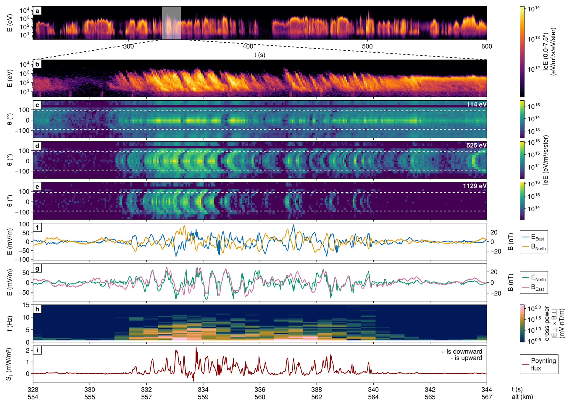
Figure 1 Data from the low-flyer (NASA 35.040) EESA and field instruments. (a–b) Differential electron energy flux over time and energy, for 0–7.5° pitch-angle. (c–e) Differential electron energy flux over time and pitch-angle, different panels correspond to different energies (114, 525 and 1129 eV) as indicated in the top right corner of each panel. (f–g) Perpendicular components of the electric and magnetic fields. DC components have been removed using a 6th-order high-pass Butterworth filter with a cut-off frequency of 0.2 Hz. (h) Cross-power spectrogram $|E_{⟂}\times B_{⟂}|$ of the perpendicular fields (short-time Fourier transform, 2 s Hann window). (i) Field-aligned Poynting flux. Positive values correspond to a downward flux into the ionosphere. The bottom axis is labelled with both flight time since launch (t) and rocket altitude (alt).

To provide context, Fig. 1a shows the differential electron energy flux measured by the low-flyer EESA, plotted over energy and time for electrons with pitch-angles of 0 to 7.5°, for the whole flight. Figure 1b–i present a subset of that data from 328 to 344 s after launch. Numerous broadband energy structures are visible between 331 and 340 s in Fig. 1b, with the shared characteristic that higher energy electrons are measured first followed by lower energy electrons, resulting in energy–time dispersions. The structures observed have peak energies ranging from a few hundred eV to a few keV and typical durations less than 0.5 s. Figure 1c, d and e show the differential electron energy flux at fixed energies (114, 525 and 1129 eV), plotted over pitch-angle and time. Horizontal white dashed lines mark pitch-angles of ±90°. Angles between these lines correspond to down-going electrons, while angles above and below correspond to up-going electrons. A band with no data is visible at 135° due to a dead channel. Numerous semicircular structures are visible in Fig. 1d and e (at 525 and 1129 eV), where field-aligned electrons are measured first, and the time-of-arrival increases with pitch-angle. These pitch-angle–time dispersions coincide with the energy–time dispersions observed in Fig. 1b. The semicircular structures are not visible in Fig. 1c (114 eV), but enhancements in the field-aligned flux (around 0°) can be observed at the same time as the structures are seen in Fig. 1d and e. Coincident electromagnetic wave activity is visible in Fig. 1f and g which present measurements from the fields instrument onboard the same rocket (E_East and B_North in panel f, E_North and B_East in panel g). The DC components have been removed using a high-pass filter with a 0.2 Hz cut-off. The cross-power spectrogram of E_⟂ and B_⟂ shown in Fig. 1h reveals broadband fluctuations in the interval between 331 and 340 s, with most of the power concentrated under ∼ 10 Hz (in the spacecraft frame). In the same time interval, panel Fig. 1i shows bursts in the downward Poynting flux (positive values), calculated from the field measurements shown in Fig. 1f and g.

A comprehensive wave analysis is beyond the scope of this paper. However, for completeness, a short cross-spectral analysis of the perpendicular fields over the 331–340 s interval is presented in Appendix A. The calculated $E_{⟂}/B_{⟂}$ ratio lies around 2500–3000 km s⁻¹ between 1 and 8 Hz, which lies close to a first-order estimation of the local MHD Alfvén speed V_A≈2730 km s⁻¹ at the rocket position and altitude (∼ 560 km). In that same frequency band, the perpendicular field pairs E_East–B_North (Fig. 1f) and E_North–B_East (Fig. 1g) present high coherence and cross-phases consistent with downward wave propagation (Wygant et al., 2000; Chaston et al., 2003a). Together with the downward field-aligned Poynting flux (Fig. 1i) and the time-dispersed electron signatures (Fig. 1b–e), these elements support an interpretation of predominantly downward-propagating Alfvén waves associated with the precipitation.

3 Dispersions fitting

In the rest of this paper, source altitudes are reported as geodetic heights above ground. Dispersion fits yield path-lengths along magnetic field lines (electron travel path), which we convert to geodetic height. For the high-latitudes and altitude ranges considered here, the difference is of around 1 % (e.g. a distance of 3000 km along a magnetic field line corresponds to an altitude above ground of approximately 2960 km).

We further note that, in the accepted picture of resonant acceleration by DAWs, electrons gain energy progressively while travelling with the wave and can therefore be transported and energized over substantial distances along magnetic field lines (Chaston et al., 2003a; Watt et al., 2006; Schroeder et al., 2021). Accordingly, the source altitudes derived from the dispersion fits are best interpreted as effective release altitudes, from which the electrons leave the resonant interaction with the wave and propagate to the rocket without further energization.

In the following sub-sections, we describe two classes of methods for estimating source altitude of Alfvénic precipitation. The first one is based on fitting energy–time dispersions, and the second uses pitch-angle–time dispersions. The combined results of both methods applied to dispersions measured by VISIONS-2 are shown in Sect. 4.

3.1 Energy–time dispersions

Estimation of source altitude through a linear fit of the time-of-flight (TOF) slope of energy–time dispersions is a method widely used in the literature (e.g. McFadden et al., 1987; Clemmons et al., 1994; Arnoldy et al., 1999; Lynch et al., 1999, 2012; Andersson et al., 2002; Tanaka et al., 2005a; Motoba and Hirahara, 2016; Hirahara et al., 2024; Feltman et al., 2025; Michell et al., 2025). It assumes that electrons of different energies are released simultaneously from a single altitude, so that differences in arrival time arise only from the differences in time-of-flight between electrons with different velocities. This assumption does not accurately represent the expected spatial and temporal characteristics of a wave-particle interaction, which is thought to happen over a wide range of altitudes as DAWs propagate downward toward the ionosphere (Kletzing and Hu, 2001). These limitations are known (e.g. Kletzing, 1994; Andersson et al., 2002; Tanaka et al., 2005a; Feltman et al., 2025), but the method remains useful as it provides a single characteristic distance that can be compared across events and studies. Using the Akaike Information Criterion (AIC), Tanaka et al. (2005a) showed that a 2nd order polynomial (quadratic curve) is frequently a better fit to the dispersion curves of the delay in arrival time Δt over the inverse of the electron velocity $(\mathrm{1}/v)$ than the classical linear fit. This suggests that the relationship between arrival time and inverse velocity is not strictly linear, which is expected if acceleration occurs over a range of altitudes rather than at a single point (Tanaka et al., 2005a). The fitted curve can then be differentiated to obtain a range of source altitudes varying with electron energy, though this still implies a simultaneous release at all energies over the range.

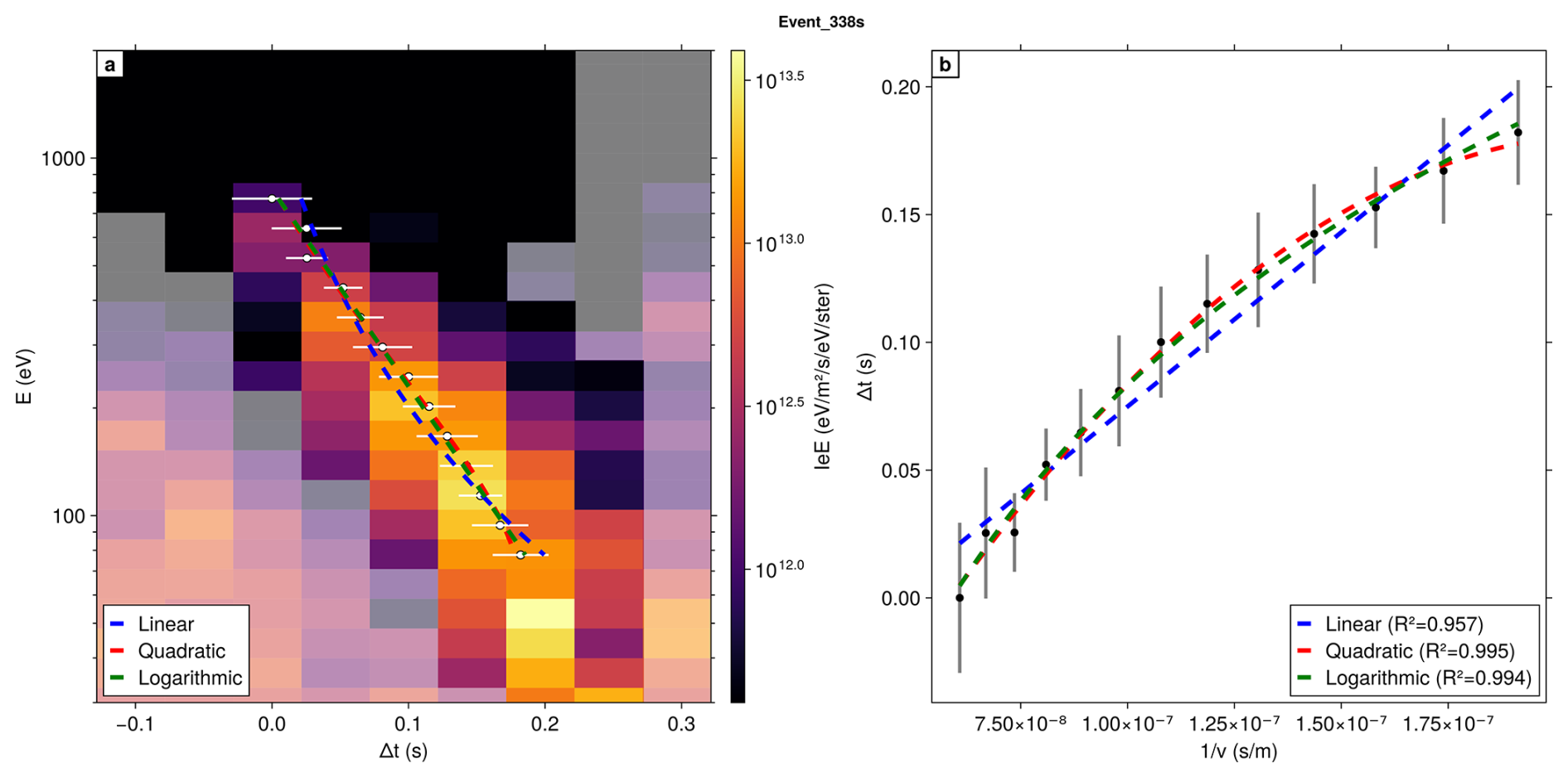
Figure 2 (a) Zoom-in on the energy-time dispersed structure visible in Fig. 1b at 338 s. Data surrounding the structure and not taken into account in the analysis are shown with a high transparency. White dots indicate the mean arrival time Δt of each energy, and the white horizontal bars indicate the width in time of the structure as given by the standard deviation around the mean. (b) Mean arrival times Δt plotted over corresponding $\mathrm{1}/v$. Gray vertical bars indicate one standard deviation as in panel (a). The blue, red and green curves in both panels indicate respectively the best linear, quadratic and logarithmic fit of Δt over $\mathrm{1}/v$.

As shown in Fig. 1, numerous distinct time–energy dispersed structures are visible in the VISIONS-2 data, to which the TOF fitting methods described above can be applied. Figure 2 presents an illustrative example using one event identified at around 338 s (Fig. 1b). Figure 2a shows the energy–time dispersed structure. Measurements on either side of the structure (displayed with higher transparency) are excluded from the analysis, as we attribute them to adjacent precipitation. For each energy slice, the electron arrival time is determined by calculating the flux-weighted mean time. These mean values are marked with white dots in Fig. 2a, and the white horizontal bars indicate the width in time of the structure as given by the square root of the weighted second moment calculated around each mean (standard deviation). Figure 2b shows the same mean arrival time, Δt, and estimated widths, plotted in Δt over $\mathrm{1}/v$ space. The blue curve shows the best linear fit of the form $\mathrm{\Delta }t=a+b(\mathrm{1}/v)$, while the red curve shows the best quadratic fit of the form $\mathrm{\Delta }t=a+b(\mathrm{1}/v)+c(\mathrm{1}/v{)}^{\mathrm{2}}$ where a, b and c are the best fit parameters, following the approach proposed by Tanaka et al. (2005a). In addition, we fit a logarithmic curve of the form $\mathrm{\Delta }t=a-b\ln (\mathrm{1}/v)$, shown in green in Fig. 2. This curve corresponds to a straight line in an energy-time space plotted on a semi-log scale such as in Fig. 2a, which seems to visually correspond well with several events in our dataset. Arrival times for energies under 70 eV are excluded from the analysis. Measurements at these lower energies are generally noisier, making the identification of well-defined peaks in arrival time more challenging. Tests made by varying the cut-off value from 50 to 100 eV did not change the overall trend of the results significantly, indicating that the analysis is not strongly sensitive to the exact value of this threshold. A more detailed discussion of this choice is provided in Sect. 4.

Following Tanaka et al. (2005a) and Feltman et al. (2025), a range of source altitudes can be estimated using the function ℱ relating Δt and $\frac{\mathrm{1}}{v}$ through $\mathrm{\Delta }t=\mathcal{F}\left(\frac{\mathrm{1}}{v}\right)$. Taking the derivative $\frac{d\mathcal{F}}{d\left(\frac{\mathrm{1}}{v}\right)}$ provides an estimate of the source distance at any given $\mathrm{1}/v$ via a local linear TOF approximation of the form $\mathrm{\Delta }t=d\frac{\mathrm{1}}{v}$, where d corresponds to the slope of the tangent of ℱ at that point. For the linear fit, this slope is constant, yielding the same source altitude for all energies. In contrast, the slope varies with $\mathrm{1}/v$ for the non-linear fits, resulting in different altitudes for different energies. Both methods, however, still rely on the assumption of an instantaneous electron release over the inferred altitude range.

3.2 Pitch-angle–time dispersions

Although the energy–time linear TOF method as described in the previous section is frequently used, fewer studies have exploited pitch-angle–time dispersions for source altitude estimation. The advantage of such a method would be that, as long as the dispersions are resolved across multiple energy channels, the source altitude can be estimated independently for each electron energy. This is a relaxation of the assumption of simultaneous release across energies that underlies the energy–time methods described in the previous section. For instance, Tanaka et al. (2005a) attempted to estimate source altitudes from the different arrival times of electrons at 0° and 30° pitch-angle, but the resulting source altitude estimates carried large uncertainties (several thousand kilometers), which were attributed to insufficient time and angular resolution. They concluded that measurements with higher resolution were necessary. The time resolution of our measurements (∼ 50 ms) is similar to theirs (∼ 41 ms), but the angular resolution of the EESA onboard VISIONS-2 (see Table A1) allows us to resolve clear pitch-angle–time dispersions across a higher number of pitch-angle channels (from −110 to 110°) as seen in Fig. 1.

Here, we test and further expand on the idea of using pitch-angle–time dispersions by developing and using a simple forward model, with two main components.

The first component simulates the propagation of electrons from a source altitude z_source to a measurement altitude z_meas. The electrons, all with the same kinetic energy, are launched simultaneously from z_source with a range of pitch-angles. The magnetic mirroring force is accounted for by conservation of the magnetic moment, using the IGRF-14 model (International Association of Geomagnetism and Aeronomy, 2024) for the magnetic field strength, which is close to a dipole field model over the heights of interest. As such, the pitch-angle is allowed to evolve along the particle trajectory, which can change the total path-length.

The second component models the detector response. A Gaussian with width σ_t is centered on the computed time-of-arrival of each electron, representing an injection at source altitude extended in time. Electrons arriving within a certain pitch-angle and time window are then integrated to produce a simulated total count for each detector pixel. The time windows are 1 ms wide and repeated every 50 ms to reproduce the behaviour of the instrumental energy sweep. The pitch-angle window widths match the angular resolution of the instrument channels. Since the absolute time of injection is unknown, a free offset parameter t_offset is applied uniformly to all arrival times.

For each energy channel, electron trajectories are computed and the three model parameters z_source, σ_t and t_offset are varied. The advantage of this approach is that, unlike with the energy-time dispersion fits, each energy bin will have an independently fit release height and time. The best fitting values are found by minimizing the sum of squared errors (SSE) between the normalized observed and modelled pitch-angle–time dispersions. Because the intensity distribution across pitch-angle in the source population is not constrained by the model, each pitch-angle channel is normalized by its total flux count before computing the SSE. This normalization also mitigates potential differences in sensitivity between pitch-angle channels in the observed data. As a result, the optimization compares only the morphology of the pitch-angle–time dispersions, rather than their absolute amplitudes.

In this work, we restrict the forward model to the down-going pitch-angle channels (−70, −45, −20, −5, 0, 5, 20, 45, 70°). As mentioned above, the dispersed structures are typically visible in a higher number of channels, from −110 to 110°, which also includes up-going channels (mirroring electrons). As a general rule, more channels lead to better constraints on the forward model. However, because the Alfvénic precipitation is strongly field-aligned, the differential flux decreases with increasing pitch-angle. Additionally, the channels of this specific EESA are narrower in angular width close to −90 and 90° (Table A1). The resulting lower signal-to-noise ratio (SNR) of these channels could potentially degrade the quality of the fits rather than improve them, and it was decided not to include them. We note that future instruments with higher sensitivity might be able to exploit the information contained in these high pitch-angle and up-going channels and further improve the quality of the results.

An example of the application of the forward model is shown in Fig. 3. The event is the same as the one whose energy–time dispersion was presented in Fig. 2, and the energy slice considered here is taken at 358 eV. Figure 3a shows the observed pitch-angle–time dispersion after normalization, while Fig. 3b presents the best-fit modelled dispersion. Figure 3c–e illustrate the variation of the SSE as a function of each of the three model parameters z_source, σ_t and t_offset, with the remaining two parameters held fixed at their best-fit values. The best-fit value of each parameter is indicated by a vertical dashed line and an annotation. Finally, Fig. 3f shows the mapping between pitch-angles at the source altitude and those at the measurement altitude for the best-fit solution. In this example, electrons measured with a pitch-angle of 60° at the rocket altitude started with a pitch-angle of approximately 40° at the inferred source altitude.

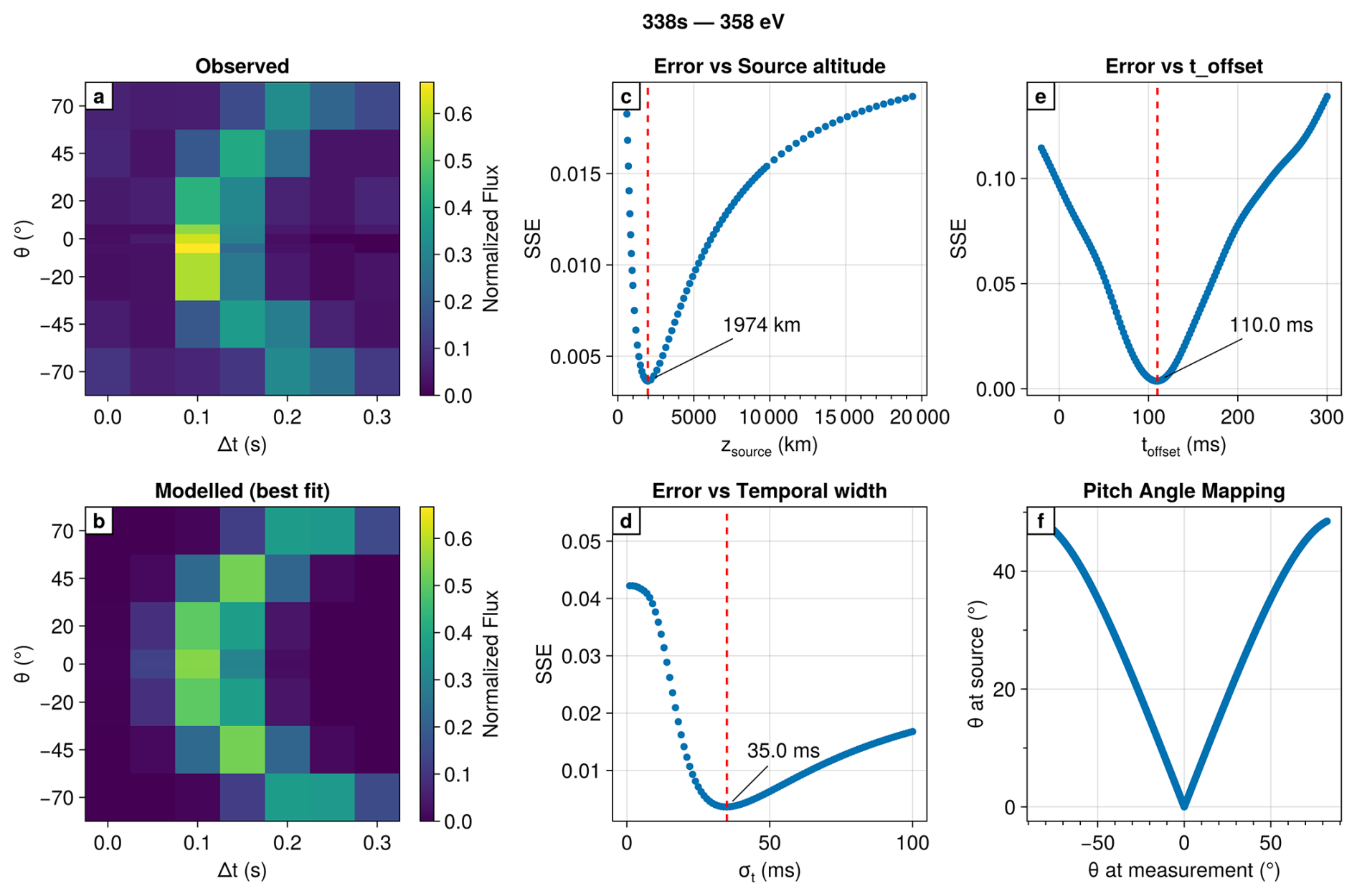
Figure 3 (a) Observed pitch-angle–time dispersion in the 358 eV slice of the event seen at 338 s in Fig. 1. The total flux in each pitch-angle channel has been normalized to 1. (b) Best-fitting simulated dispersion by the forward model, as found by the minimization of the SSE. (c) Variation of the SSE over the parameter z_source, for the best values of σ_t and t_offset. (d) Variation of the SSE over the parameter σ_t for the best values of z_source and t_offset. (e) Variation of the SSE over the parameter t_offset for the best values of z_source and σ_t. (f) Relation between the pitch-angle of electrons at the source altitude and measurement altitude.

Once the best-fitting parameters are found, the uncertainty in the estimated source altitude is obtained through a linearised uncertainty estimation (Aster et al., 2019). The parameter covariance matrix Σ_p is calculated as

$${\mathrm{\Sigma }}_{\mathrm{p}}={\mathit{\sigma }}_r^{\mathrm{2}}(J^{T}J{)}^{-\mathrm{1}}$$

where σ_r is the root mean square difference between the observed and best-fit modelled dispersions, and J is the Jacobian matrix of the model evaluated around the best-fit parameters. The standard error on the source altitude is then the square root of the first diagonal element of Σ_p.

4 Source altitudes

We now apply the energy–time and pitch-angle–time dispersion fitting methods as described in the previous section to events measured by the rocket. Figure 4a shows the source altitude as a function of electron energy found with the different methods applied to the event at 338 s. This is the event that was used to describe the fitting methods in Figs. 2 and 3. Figures 4b–f show results from other dispersed events, whose time in flight is indicated in the top-right corner of each panel. The blue, red, and green curves show results from respectively the linear, quadratic, and logarithmic energy–time TOF fits. For each event, the source altitude curve inferred from the best fitting model is indicated with a solid line while curves from the two others are dashed. Determining the best fitting model was done using the corrected Akaike Information Criterion (AICc) (Sugiura, 1978):

$$\begin{array}{}\text{(1)}& \mathrm{AICc}=\mathrm{AIC}+{\displaystyle \frac{\mathrm{2}{k}^{\mathrm{2}}+\mathrm{2}k}{n-k-\mathrm{1}}}\end{array}$$

where AIC $=\mathrm{2}k+n\ln \left(\mathrm{RSS}/n\right)$ is the standard Akaike Information Criterion (Akaike, 1974) with unknown variance, RSS is the residual sum of squares, n is the number of data points, and k is the number of parameters in the model being fitted (e.g. 3 for the quadratic fit: a, b and c). We use the AICc correction in place of the AIC as the number of data points per event is small (regularly fewer than 15), which can cause the standard AIC to overly favour complex models (Cavanaugh and Neath, 2019).

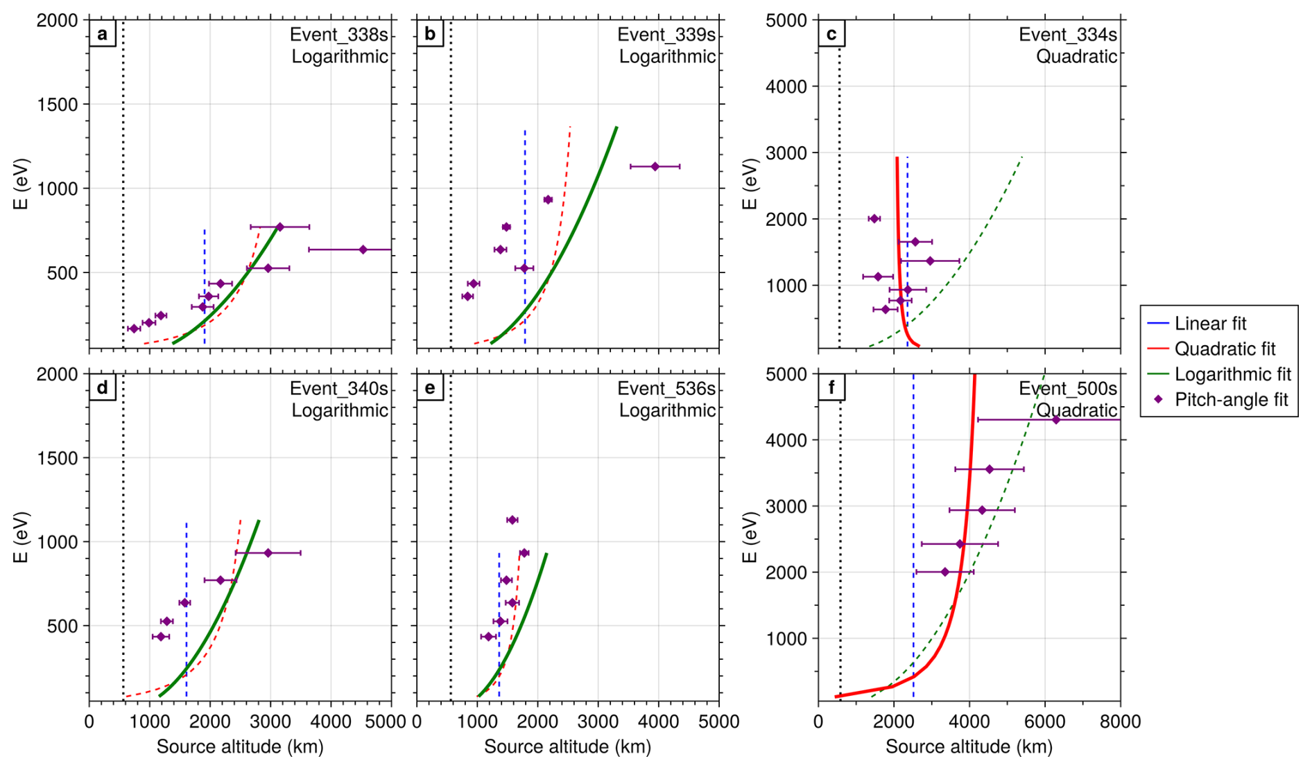
Figure 4 Results of the energy–time dispersion and pitch-angle–time dispersion analysis on a subset of events where both methods were applied. Each panel shows a different event whose time in the flight is indicated in the top-right corner. The blue, red and green curves indicate the source altitude as a function of energy for the linear, quadratic and logarithmic fits of the energy–time dispersions, respectively. The best model as found with the AICc is indicated in each panel with a solid line, while the two others are indicated by dashed lines. In addition, the name of the best model is also indicated in the top-right corner of each panel. Purple points indicate source altitude found with the pitch-angle–time dispersion modelling. Error bars indicate ±1 standard error in the source altitude estimation. The rocket altitude is shown in each panel with a vertical dotted black line.

The purple points show source altitudes estimated from the pitch-angle–time dispersion forward model, with error bars representing ±1 standard error. Results from the pitch-angle–time analysis generally follow those from the energy–time analysis across events, despite the two methods relying on different assumptions: the energy–time method assumes instantaneous release of field-aligned electrons at all energies over a range of altitudes, while the pitch-angle method assumes an independent release at each energy, but with a broader pitch-angle distribution. When departures are visible (e.g. the 339 s event shown in Fig. 4b), the differences in source altitude rarely surpass 1000 km. This relatively good agreement between the two types of methods strengthens the confidence in the estimated source altitudes.

We observe variations in the range of source altitudes between events. For example, clear differences are visible between the 338 s event (Fig. 4a) and the 334 s event (Fig. 4c). The 338 s event is best represented by a logarithmic fit, with source altitudes spanning a wider range (1400 to 3000 km). By contrast, the 334 s event is best represented with a quadratic fit very close to the linear fit, suggesting a narrow range of source altitudes (around 2200 km) across all energies, consistent with results from the pitch-angle analysis. For this event, the quadratic fit is slightly concave, i.e. its coefficient c is negative and it bends in the other way than for the other events visible in Fig. 4. This is consistent with the observations of Tanaka et al. (2005a) finding the quadratic curves to be in general convex, but with a few events being concave close to linear.

The general trend across events is that the source altitude increases with electron energy. For all events, the fitted t_offset parameter from the pitch-angle analysis tends to increase (not shown here) with the inverse of the electron energy, indicating a later time of release for the lower energy electrons. This is consistent with the source altitude profiles shown in Fig. 4 and the picture of a wave travelling down along the magnetic field line.

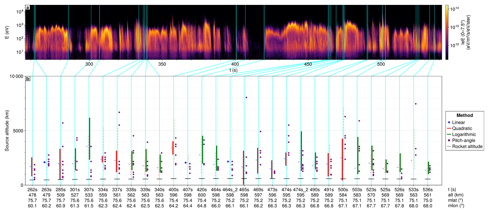
Figure 5 Summary of inferred source altitudes across 29 analysed events. (a) Differential electron energy flux over time and energy as measured by the low-flyer EESA (0–7.5° pitch-angle). Cyan bands mark the time span of each analysed event and are connected to the corresponding event columns in panel (b). (b) Source altitudes per event obtained from the different methods. The blue crosses indicate the result from linear fit. The red and green lines indicate the range of source altitudes found from the quadratic and logarithmic fits, respectively. The preferred model as found with the AICc is indicated with thicker lines and crosses. The purple dots indicate the source altitudes found with the pitch-angle method. The rocket altitude at the time of each measurement is indicated by a thin horizontal black line. The geomagnetic coordinates on the x-axis are computed from the geographic coordinates of the rocket and the geomagnetic pole (dipole approximation) location from IGRF-14.

In Fig. 5, we show a summary of the source altitude estimations across a large number of events for which energy–time and pitch-angle–time dispersions were easy to distinguish visually. Results from different energies are mixed, and the time of each event is indicated on the x-axis. Blue crosses show the source altitude from the linear TOF. Red and green lines indicate the range of source altitude from the quadratic and logarithmic fits, respectively. For each event, the preferred model according to the AICc is indicated with thicker lines and crosses. Purple dots show the source altitudes inferred from the pitch-angle forward model, and short horizontal bars indicate the rocket altitude at the time of the measurements.

With $\mathrm{12}/\mathrm{29}$ events best fitted by a quadratic curve, $\mathrm{14}/\mathrm{29}$ events best fitted by a logarithmic curve, and $\mathrm{3}/\mathrm{29}$ events best fitted by a linear curve, we observe that the non-linear fits are generally preferred to the linear fit, consistent with the findings of Tanaka et al. (2005a) and Feltman et al. (2025). Varying the lower energy cut-off described in Sect. 3.1 (set at 70 eV for the results shown in Fig. 5) with values from 50 to 100 eV causes the preferred curve model for some events to change. The general distribution of the favoured models and the range of source altitudes for each event is however generally unchanged.

It can be observed that for some events, the quadratic model infers source altitude for low-energy electrons below the rocket altitude, which is unphysical. This occurs because the local derivative of the quadratic $\mathrm{\Delta }t(\mathrm{1}/v)$ curve can become negative at high $\mathrm{1}/v$ values, yielding negative source distances at the lowest energies.

As already noted with the few events presented in Fig. 4, we also observe that the range of source altitudes found with the pitch-angle method generally agrees with those from the energy TOF methods, though some outliers at lower and higher altitudes are visible. We also notice that the grand majority of source altitudes found across events lie lower than 5000 km, frequently between 1000 and 3000 km. We will discuss these findings in the light of other studies and theoretical expectations in the next section.

5 Discussion

5.1 Reliability of the source altitude estimations

To infer at which altitude the acceleration of the electrons took place, we have used two types of methods, one based on energy–time dispersions and one on pitch-angle–time dispersions. Both approaches are subject to uncertainties, which we discuss below.

The first source of uncertainty relates to the finite resolution of measurements. The energy–time dispersions methods rely on fitting the arrival times of electrons at different energies. However, as can be seen in Fig. 2, the observed structures are often only a few pixels wide in time at each energy. Although we mitigate this by calculating a weighted mean, the limited time resolution still introduces uncertainty on the precise arrival time of each energy. We expect a higher temporal resolution to better constrain the dispersion fits and the inferred source altitudes. Similarly, the pitch-angle–time dispersion method is also affected by measurement resolution. This is visible in Fig. 4, where the uncertainties generally increase with source altitude (e.g. the large error bars in the 500 s event in Fig. 4f). This reflects the reduced sensitivity of the pitch-angle–time dispersion shape to source altitude at large distances. Higher resolution measurements in both time and pitch-angle would better constrain the forward model and reduce these uncertainties.

A second source of uncertainty concerns the interpretation made of the dispersed structures themselves: do they reflect temporal variations in the precipitation, or spatial structures sampled by the moving spacecraft. This distinction is a long-standing question in in-situ observational studies of auroral precipitation (e.g. Tanaka et al., 2005a; Wu et al., 2021). During the measurements, the rocket had a horizontal velocity of 1–2 km s⁻¹, implying that it covered spatial distances of roughly 0.5 to 1 km over the typical duration of these structures (< 0.5 s). Previous multi-point measurement studies have reported simultaneous measurement of similar precipitation signatures across payloads separated by ∼ 0.9–3 km (Arnoldy et al., 1999; Lynch et al., 1999, 2012), suggesting that these structures extend over larger spatial scale than the displacement of the rocket and therefore supporting a temporal interpretation. In addition, the coincident observation of dispersions in both energy and pitch-angle (Fig. 1) further strengthens a temporal origin (Arnoldy et al., 1999), as a purely spatial interpretation would imply simultaneous change across all pitch-angles.

A third source of uncertainty arises from the assumptions underlying each method. When deriving source altitudes from the energy–time dispersion fits, it is assumed that field-aligned electrons are released simultaneously over the whole source region, which is not fully consistent with the expected picture of a moving wave-particle interaction (Andersson et al., 2002). For the linear fit case, commonly used in the literature, this release is further assumed to occur from a single point. Similar to Tanaka et al. (2005a) and Feltman et al. (2025), we find that the non-linear fits of the energy–time dispersions are generally preferred over the linear fits, supporting the case of a wider range of source altitude. Nevertheless, we also observe that the point source altitudes inferred from the linear fits typically fall near the middle of the altitude ranges derived from the non-linear fits (Figs. 4, 5). As such, it seems that the linear fit can provide a convenient first-order estimate, straightforward to compute, and that can be used for a quick comparison across events and studies.

In order to relax the assumption of simultaneous release associated with the energy–time dispersion fits, we developed and applied a second method based on the pitch-angle–time dispersions. This approach allows the source altitude to be estimated independently for each electron energy, and instead assumes the instantaneous release of a broader pitch-angle distribution. We expect this assumption to be more accurate the higher the source altitudes. Indeed, at greater source distances, the injected electrons have a narrower pitch-angle distribution and are therefore more likely to originate from a similar altitude. For instance, the source altitude of the 4300 eV electrons of the 500 s event (Fig. 4f) is inferred to be around 6400 km, with pitch-angles at the source ranging from 0 to 25°, meaning that all the electrons had a field-aligned velocity component between cos (25°)≈0.9 and 1 of their total speed.

Despite the aforementioned uncertainties, we found both approaches, each with different underlying assumptions regarding electron injection, to yield comparable ranges of source altitudes across events (Figs. 4 and 5). This agreement between the two types of methods increases confidence in the inferred source altitudes.

5.2 Source altitudes in the context of previous studies

Having discussed the robustness and validity of the inferred source altitudes, we now examine how these results compare with previous observational studies and theoretical expectations.

The source altitudes inferred both from the energy–time and pitch-angle–time dispersions methods show some variability across events (Figs. 4 and 5), despite being observed during the same rocket flight. This suggests differences in plasma conditions and/or wave parameters along nearby magnetic field lines. Whether these differences arise from local temporal variations or a larger spatial structuring of the acceleration region remains unclear due to space-time ambiguities that cannot be resolved with a single sounding rocket. It is expected that conditions along field lines can evolve following earlier auroral precipitation (Chaston et al., 2000, 2003b, 2006), but also that these regions can present strong spatial structuring, such as in the ionospheric Alfvén resonator (IAR) (Streltsov and Lotko, 2008).

Despite this variability, our observations generally indicate source altitudes of ∼ 1000–3000 km for electrons with energies of a few hundred eV, and ∼ 2000–5000 km for electrons with energies of a few keV. The general trend is for high-energy electrons to be released at higher altitudes than low-energy electrons, consistent with expected Alfvén velocity profiles along magnetic field lines (Chaston et al., 2002a). However, these values lie on the lower end of theoretical predictions (e.g. Kletzing and Hu, 2001; Chaston et al., 2003a), especially for the dayside (Chaston et al., 2003b).

For comparison, from their observations also made on the dayside at a similar MLT (around 13.3 MLT) with a sounding rocket, Tanaka et al. (2005a) inferred source altitudes of ∼ 2000–3000 km for ∼ 30 eV electrons and ∼ 5000–6000 km for ∼ 200 eV electrons using a non-linear (quadratic) fit method. These values are more consistent with the theoretical estimations of Chaston et al. (2003b). However, the maximum electron energies in their dispersed structures were generally lower (a few hundred eV) than in our observations (up to several keV), suggesting different plasma and wave conditions in the acceleration-region between our studies.

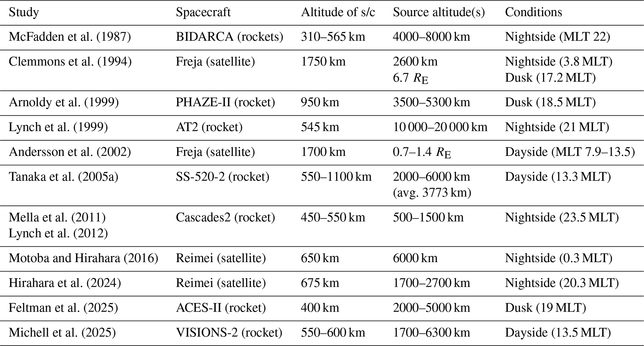
When compared with source altitudes reported in previous studies (Table 1) from linear fits of energy–time dispersions, our results also fall on the lower end of the observed range. Using the same linear fitting approach, our estimates typically lie between 1000 and 3000 km (blue crosses in Fig. 5). However, similar source altitudes have been reported in Hirahara et al. (2024) as well as Mella et al. (2011) and Lynch et al. (2012) for events measured on the nightside and reaching several keV. For comparison with the other results reported in Table 1, the VISIONS-2 rocket was at altitudes between 480 and 600 km and around a MLT of 13.5 during the observations of Fig. 5.

McFadden et al. (1987)Clemmons et al. (1994)Arnoldy et al. (1999)Lynch et al. (1999)Andersson et al. (2002)Tanaka et al. (2005a)Mella et al. (2011)Lynch et al. (2012)Motoba and Hirahara (2016)Hirahara et al. (2024)Feltman et al. (2025)Michell et al. (2025)

Table 1 Comparison of source altitudes across studies found with the linear fit method of energy–time dispersions (MLT: Magnetic Local Time).

The results of Michell et al. (2025) were obtained using data from the Acute Precipitating Electron Spectrometer (APES) instrument (Michell et al., 2016) onboard the same rocket as in our study. By design, their instrument resolves primarily the highest energy part of the dispersions (Michell et al., 2025). The source altitudes of the 8 events they report range from approximately 1700 to 6300 km, which is consistent with the higher-energy portion of the source altitudes we inferred from the non-linear energy fits and pitch-angle approaches presented here.

Overall, the wide range of source altitudes reported across studies (Table 1), from ∼ 500 km to several R_E, does not appear to clearly correlate with the spacecraft type (rocket vs. satellite), the spacecraft altitude, or the magnetic local time (MLT) of observations. Similar to the event-to-event variations observed in our data, these differences suggest different plasma and wave conditions along the magnetic field lines.

To further interpret our inferred source altitudes in terms of the plasma environment along the magnetic field lines, we compare our observations with theoretical expectations derived from different plasma density profiles in the acceleration region reported in the literature. Figure 6a shows the density profiles. All the profiles are based on the combination of an ionospheric exponential law for O⁺ and a magnetospheric power-law component for H⁺, with different parametrizations. The parametrizations of Kletzing et al. (1998), Chaston et al. (2002a) and Chaston et al. (2003a) result from statistical fits to spacecraft observations, whereas the parameters used by Thompson and Lysak (1996) and Lysak and Song (2008) were chosen to study specific plasma environments. In particular, the two profiles from Lysak and Song (2008) represent conditions inside and outside a density cavity. Figure 6b shows the magnetic field strength along the field line passing through the general rocket measurement region (taken at 76° N, 3° E and 100 km altitude), computed using the IGRF-14 model (International Association of Geomagnetism and Aeronomy, 2024). Figure 6c and d show the corresponding electron skin-depth ${\mathit{\lambda }}_{\mathrm{e}}=c/{\mathit{\omega }}_{\mathrm{p}}$ and Alfvén velocity profiles (solid lines), together with inertial Alfvén wave velocity profiles (dashed lines). The inertial Alfvén velocities were computed assuming a perpendicular wavelength ${\mathit{\lambda }}_{⟂\mathrm{0}}=\mathrm{5}$ km at 200 km altitude (following Chaston et al., 2002a), scaled with $\mathrm{1}/\sqrt{B}$ under the assumption of constant magnetic flux. This perpendicular scale should correspond to auroral structures with optical widths of ∼ 1–2 km (Chaston et al., 2002a, 2003b). Figure 6e compares these theoretical profiles with the source altitudes inferred from our observations, with the inertial Alfvén wave velocities expressed as equivalent electron kinetic energies $E=\frac{\mathrm{1}}{\mathrm{2}}{m}_e{v}_{\mathrm{AI}}^{\mathrm{2}}$, which corresponds to the assumption that electrons are accelerated to approximately the local inertial Alfvén speed. As discussed in the introduction, theoretical and modelling studies have shown that electrons can be accelerated through resonant interaction to parallel velocities greater than 1V_A, up to $\mathrm{2}{V}_{\mathrm{A}}-v_{{\parallel }_{\mathrm{0}}}$ (e.g. Kletzing, 1994; Kletzing and Hu, 2001; Chen et al., 2005; Watt et al., 2005, 2006), while we also expect electrons within the resonance window defined by the wave parallel electric field E_∥ to be possibly released before reaching the wave speed, i.e. at energies slightly below 1V_A. The curves of Fig. 6e should therefore be regarded as characteristic equivalent energies rather than strict bounds. The scatter points represent all source altitude estimates from Fig. 5 as a function of electron energy, derived from the pitch-angle method (purple), the quadratic fit (red), and logarithmic fit (green).

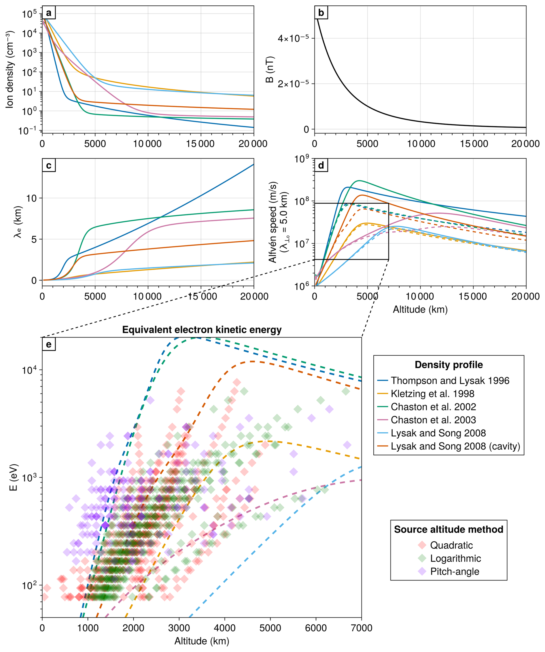
Figure 6 (a) Profiles of plasma density from the literature. (b) Profile of the magnetic field strength along the magnetic field line going through a point at 76° of latitude, 3° of longitude and 100 km of altitude, which corresponds to the region where the rocket is situated during the measurements. (c) Profiles of the electron skin-depth ${\mathit{\lambda }}_{\mathrm{e}}=c/{\mathit{\omega }}_{\mathrm{p}}$ obtained from the different density profiles. (d) Profiles of the corresponding Alfvén velocity (solid lines) and inertial Alfvén wave velocity (dashed lines). The inertial Alfvén wave velocities were calculated assuming a perpendicular wavelength of the wave λ_⟂0 of 5 km (similar to Chaston et al. (2002a)) at 200 km of altitude, then scaled in altitude with $\mathrm{1}/\sqrt{B}$ (constant magnetic flux assumption). (e) Zoom-in section of the velocity profiles from panel d. Only the inertial Alfvén waves profiles are shown. The y-axis values show what would be the equivalent kinetic electron energy calculated from $E=\frac{\mathrm{1}}{\mathrm{2}}{m}_e{v}_{\mathrm{AI}}^{\mathrm{2}}$. The scatter points show a compilation of all the source altitudes found as a function of energy for all the events shown in Fig. 5 for the pitch-angle method (purple), quadratic fit (red) and logarithmic fit (green). All the results are mixed.

Using the parameters described above, the inferred source altitudes from our events are consistent with the IAW velocities predicted using the density profiles of Thompson and Lysak (1996), Kletzing et al. (1998), Chaston et al. (2002a), and the cavity profile of Lysak and Song (2008). A smaller number of events are also consistent with the profile of Chaston et al. (2003a), which is the results of a statistical fitting of dayside measurements. In contrast, almost none of our source altitudes follow the outside-cavity conditions profile of Lysak and Song (2008). Taken together, the source altitudes inferred from our events are most consistent with profiles with the lowest O⁺ scale heights, leading to a transition to H⁺ dominated plasma at lower altitudes. If the plasma on surrounding field lines has a higher O⁺ scale height, e.g. as in the statistically fitted dayside profile from Chaston et al. (2003a), measurements from a satellite horizontal fly-by would resemble a locally depleted density region. This picture would be consistent with previous studies reporting observations from satellites between 1000 and 4000 km of altitude of Alfvén waves propagating inside density cavities and carrying intense parallel electric fields (Chaston et al., 1999, 2000, 2006, 2007b). The coupling between density cavities, Alfvén waves, and intense parallel electric fields has indeed been investigated and seemingly established in numerical studies (Génot et al., 2004; Lysak and Song, 2008; Mottez and Génot, 2011).

The comparison between inferred release altitudes and the Alfvén-wave phase velocity profiles of Fig. 6 suggests it is possible to fit the inferred energy, time, and height obtained from the pitch-angle dispersion fits described in Sect. 3.2 to the acceleration region parameters that influence the inertial Alfvén wave velocity: O⁺ and H⁺ density profiles and perpendicular wavelength. We can build such a fit assuming a plasma density profile in the topside ionosphere of the following form (Lysak and Song, 2008)

$$\begin{array}{}\text{(2)}& {\displaystyle }{n}_{O^{+}}=n_{\mathrm{0}}{e}^{-z/H}\text{(3)}& {\displaystyle }{n}_{H^{+}}=n_{\mathrm{1}}{\left({\displaystyle \frac{z+R_{\mathrm{E}}}{R_{\mathrm{E}}}}\right)}^{-\mathrm{1}}\text{(4)}& {\displaystyle }{n}_e=n_{{\mathrm{O}}^{+}}+n_{{\mathrm{H}}^{+}}\end{array}$$

with n₀ the O⁺ density constant, n₁ the H⁺ density constant, H the scale height of O⁺, R_E the radius of the Earth, and z the geodetic height (vertical distance above ground). Quasi-neutrality is assumed, so that the electron density n_e is determined by the total ion density. The inertial Alfvén speed is defined as

$$\begin{array}{}\text{(5)}& v_{\mathrm{AI}}={\displaystyle \frac{V_{\mathrm{A}}}{\sqrt{\mathrm{1}+k_{⟂}^{\mathrm{2}}{\mathit{\lambda }}_{\mathrm{e}}^{\mathrm{2}}}}}\end{array}$$

where $V_{\mathrm{A}}=B/\sqrt{{\mathit{\mu }}_{\mathrm{0}}(n_{O^{+}}{m}_{O^{+}}+n_{H^{+}}{m}_{H^{+}})}$ is the pure MHD Alfvén velocity determined by O⁺ and H⁺ mass density and the IGRF magnetic field strength B, and ${\mathit{\lambda }}_{\mathrm{e}}=c/\sqrt{n_e{e}^{\mathrm{2}}/m_e{\mathit{ϵ}}_{\mathrm{0}}}$ is the plasma skin-depth. The perpendicular wavenumber

$$\begin{array}{}\text{(6)}& k_{⟂}={\displaystyle \frac{\mathrm{2}\mathit{\pi }}{{\mathit{\lambda }}_{⟂\mathrm{0}}}}\sqrt{{\displaystyle \frac{B}{B_{\mathrm{0}}}}}\end{array}$$

is fixed by a perpendicular wavelength λ_⟂0 and magnetic field strength B₀ defined at an altitude of 200 km and scaled by $\mathrm{1}/\sqrt{B}$ assuming constant magnetic flux.

For each event, the pitch-angle fit provides independent release altitude estimates z_i for energy bins E_i. We assume that the release height of a discrete burst of Alfvénic precipitation with energy E is initiated at an altitude where the electron energy is matched to the equivalent inertial Alfvén velocity, i.e., $Z(E,n_{\mathrm{0}},n_{\mathrm{1}},H,{\mathit{\lambda }}_{⟂\mathrm{0}})=\arg {min}_z|E-\frac{\mathrm{1}}{\mathrm{2}}{m}_e{v}_{\mathrm{AI}}^{\mathrm{2}}(z,n_{\mathrm{0}},n_{\mathrm{1}},H,{\mathit{\lambda }}_{⟂\mathrm{0}}\left)\right|$. This definition adopts the simplifying assumption that electrons leave the resonant interaction when their parallel speed is equal to the local inertial Alfvén velocity (v_AI). In reality, the resonance window allows electrons to leave the interaction with speeds higher ($\mathrm{2}{V}_{\mathrm{A}}-v_{{\parallel }_{\mathrm{0}}}$) or lower than v_AI. An inferred source altitude should therefore probably more accurately be interpreted as an effective release altitude representing a finite local range of altitudes rather than a unique point. Under this approximation of release at 1 v_AI, it is now possible to search for plasma and wave parameters that best match the calculated source altitudes by minimizing the variance weighted sum of squares:

$$\begin{array}{}\text{(7)}& \begin{array}{rl}({\widehat{n}}_{\mathrm{0}},{\widehat{n}}_{\mathrm{1}},\widehat{H},{\widehat{\mathit{\lambda }}}_{⟂\mathrm{0}})& =\begin{array}{c}\arg \min \\ n_{\mathrm{0}},n_{\mathrm{1}},H,{\mathit{\lambda }}_{⟂\mathrm{0}}\end{array}\sum _i{\mathit{\sigma }}_i^{-\mathrm{2}}\left|z_i\right.\\ & {\left.-Z(E_i,n_{\mathrm{0}},n_{\mathrm{1}},H,{\mathit{\lambda }}_{⟂\mathrm{0}})\right|}^{\mathrm{2}}\end{array}\end{array}$$

where σ_i is the error standard deviation for the source height of energy bin i (error bars in Fig. 4), and $({\widehat{n}}_{\mathrm{0}},{\widehat{n}}_{\mathrm{1}},\widehat{H},{\widehat{\mathit{\lambda }}}_{⟂\mathrm{0}})$ are the values of the best fit parameters.

The parameters n₀, n₁, and H describe the background plasma density profile, while λ_⟂0 is the only fitted wave parameter. Other wave parameters (e.g. Poynting flux, frequency) as well as characteristics of the electron source population being accelerated (e.g. density, temperature) are expected to affect the morphology of the observed electron dispersions, notably their width, total intensity and maximum energy. However, of these quantities, only the background density and perpendicular wavelength enter the inertial Alfvén speed profile as given by Eq. (5). Consequently, we expect these latter parameters to dominantly influence the curvature/slope of the electron dispersions and as such their fits and the inferred release altitudes. Results from test-particle modelling performed by Tanaka et al. (2005b) seem to support this hypothesis as only variations in the wave perpendicular scale out of several wave parameters were found to significantly modify time–energy dispersion fits.

Figure 7 shows this fitting technique applied to the pitch-angle estimated source altitudes of the 338 s event (same event as in Figs. 2, 3, and 4a). Figure 7a shows the inferred source altitudes and their associated uncertainties (similar to Fig. 4a). The black curve corresponds to the best fitting IAW speed curve to the points following Eq. (7). The values of the best curve parameters are indicated in the top right corner of the panel, with the (25th, 75th) percentile interval of the accepted parameter set given in brackets. The accepted parameter set is defined by sampling the four fit parameters ($(n_{\mathrm{0}},n_{\mathrm{1}},H,{\mathit{\lambda }}_{⟂\mathrm{0}})$) directly from the error landscape explored by the grid search. Retained are all the parameter combinations whose weighted sum of squares (Eq. 7) satisfies $S<S_{\text{min}}+\mathrm{\Delta }S$ with ΔS=4, and each combination is weighted by $\exp (-(S-S_{\text{min}})/\mathrm{2})$. The faint grey curves correspond to 250 parameter sets drawn in this way. For this event, the fitted parameters are remarkably close to the values of the profiles from previous studies shown in Fig. 6, as well as expected perpendicular IAW scales (Chaston et al., 2003b). The density profiles of O⁺ and H⁺ and $n_{\mathrm{tot}}=n_{O^{+}}+n_{H^{+}}$ along the field line can be reconstructed from the best fitting parameters following Eqs. (2) and (3), as is shown in Fig. 7b. The thick solid green line and the dashed blue and yellow lines correspond to the best fit (thick solid black line in Fig. 7a), while the faint green lines correspond to the 250 sampled parameter sets (faint black profiles in Fig. 7a). The fitting technique was applied to all the events shown in Fig. 5, and approximately two-thirds of the cases were found to have fairly good, constrained fits as in Fig. 7, while the others remained less well constrained.

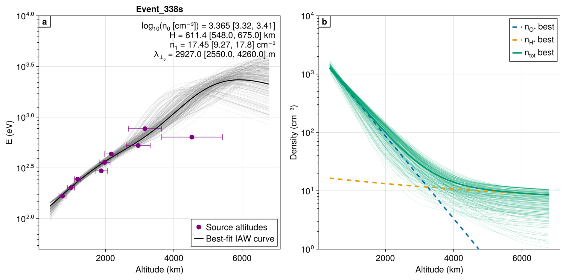
Figure 7 (a) Best-fit IAW speed profile (black curve) to the source altitudes estimated with the pitch-angle method applied to the event at 338 s. The best-fit values of the plasma and wave parameters are indicated in the top-right corner, with the (25th, 75th) percentile interval given in brackets of 250 parameter sets sampled from the fit-error landscape. The faint grey curves correspond to IAW speed profiles of the sampled parameter sets. (b) Reconstructed density profiles corresponding to the best-fit parameters of panel a, with faint curves showing the total density of the sampled parameter sets.

The parameter estimation presented here is based on the simplified assumption that electrons are accelerated to 1 V_A and that the density profiles follow the forms of Eqs. (2) and (3). Future work should determine the most appropriate acceleration assumptions and profile shapes, and assess whether this fitting approach can reliably infer topside plasma structuring.

We also want to highlight that the method relies on source-altitude estimates extracted from pitch-angle–time dispersions seen in multiple energy channels and that it therefore requires sufficient resolution in energy, time and, importantly, pitch-angle, as discussed in Sect. 5.1. As such, future missions carrying instruments with higher resolution could improve the precision of the inferred profiles. It could also be of interest to apply the technique on measurements from both rockets and satellites, where short-duration sounding rockets with state-of-the-art high-resolution instrumentation could provide tightly constrained profiles for individual auroral events, whereas satellite measurements may trade some accuracy for repeated observations over longer intervals and across a wider range of geomagnetic conditions and locations.

Both strategies would provide valuable information about the acceleration region, and the method presented here could become one of the few observation techniques capable of constraining plasma density profiles near the transition between O⁺ and H⁺ dominated plasma. Repeated measurements could then help characterize the spatial and temporal variability of this poorly sampled region of the auroral topside ionosphere.

6 Conclusions

In this study, we estimated the source altitude of auroral precipitation observed by the EESA top-hat instrument onboard the low-flyer of the VISIONS-2 sounding rocket campaign, launched on 7 December 2018 from Ny-Ålesund, Svalbard, into the active dayside auroral region (∼ 13.5 MLT). Numerous dispersed structures typical of auroral precipitation related to DAWs were observed. Their source altitudes were inferred using the standard linear fit of energy–time dispersions which assumes a point release, but also using non-linear fits to obtain ranges of source altitude varying with energy. The non-linear curves were found to generally better fit the dispersions according to the AICc, similar to the findings of Tanaka et al. (2005a), and supporting the hypothesis of an acceleration occurring across a range of altitudes.

In order to relax the assumption of simultaneous release of electrons from the whole range of source altitudes that is inherent to the energy–time dispersions fitting methods, we also developed a source altitude estimation method based on the forward modelling of pitch-angle–time dispersions. Using both complementary approaches, we obtained similar ranges of source altitudes despite the different underlying assumptions. We observed a common trend across events of higher energies mapping to higher source altitudes. Despite some variation across events, we calculated around 70 % of the source altitudes of our observations inferred with the pitch-angle method to lie between 1000 and 3000 km (Figs. 5 and 6e), for electrons with energies from hundreds of eV to a few keV. The variations in source altitudes observed across events suggest different plasma and wave conditions along the magnetic field lines where auroral acceleration takes place.

Although on the lower end, the source altitudes we found generally agree with previous observations (Table 1) and theoretical profiles of the IAW velocity (Fig. 6), especially those related to plasma density profiles with lower O⁺ scale heights. The method discussed in Sect. 5.2 opens the possibility to identify the best-fitting parameters for each event, and to extract the corresponding density profiles and perpendicular wave scale. This, combined with instrumental advancements offering higher-resolution measurements (e.g. Michell et al., 2016; Saito et al., 2017), could provide new clues about the plasma structures and processes occurring in the acceleration region.

Appendix A: Cross-spectral analysis of the perpendicular fields

Over the 331–340 s interval seen in Fig. 1, a short-time Fourier transform is applied to the perpendicular fields (2 s Hann windows, 75 % overlap, Δf≈0.5 Hz, ∼ 28 segments). The ratio $E_{⟂}/B_{⟂}$ is computed as the rotation-invariant total perpendicular power, $\sqrt{\langle |E_{\mathrm{North}}{|}^{\mathrm{2}}+|E_{\mathrm{East}}{|}^{\mathrm{2}}\rangle /\langle |B_{\mathrm{North}}{|}^{\mathrm{2}}+|B_{\mathrm{East}}{|}^{\mathrm{2}}\rangle }$, where 〈⋅〉 denotes averaging over segments. The magnitude-squared coherence γ²(f) and the cross-phase are computed for the two perpendicular field pairs, $E_{\mathrm{East}}/B_{\mathrm{North}}$ and $E_{\mathrm{North}}/B_{\mathrm{East}}$. The local Alfvén speed $V_{\mathrm{A}}=B/\sqrt{{\mathit{\mu }}_{\mathrm{0}}\mathit{\rho }}$ is evaluated from an IRI density profile (Bilitza et al., 2022) produced at the rocket location (using the full ion composition for the mass density ρ) and the IGRF-14 field strength (International Association of Geomagnetism and Aeronomy, 2024) along the traced field line, giving V_A≈2730 km s⁻¹ at the rocket altitude (∼ 560 km).

In the ∼ 1–8 Hz band (shaded in Fig. A1), $E_{⟂}/B_{⟂}\approx \mathrm{2500}$–3000 km s⁻¹ closely matches V_A (panel a), the perpendicular fields are coherent (panel b), and cross-phases lie close to 0 and 180° (panel c). Above ∼ 10 Hz the magnetic perturbation sinks into the magnetometer noise floor: the coherence collapses, the cross-phase randomises, and the ratio diverges from V_A.

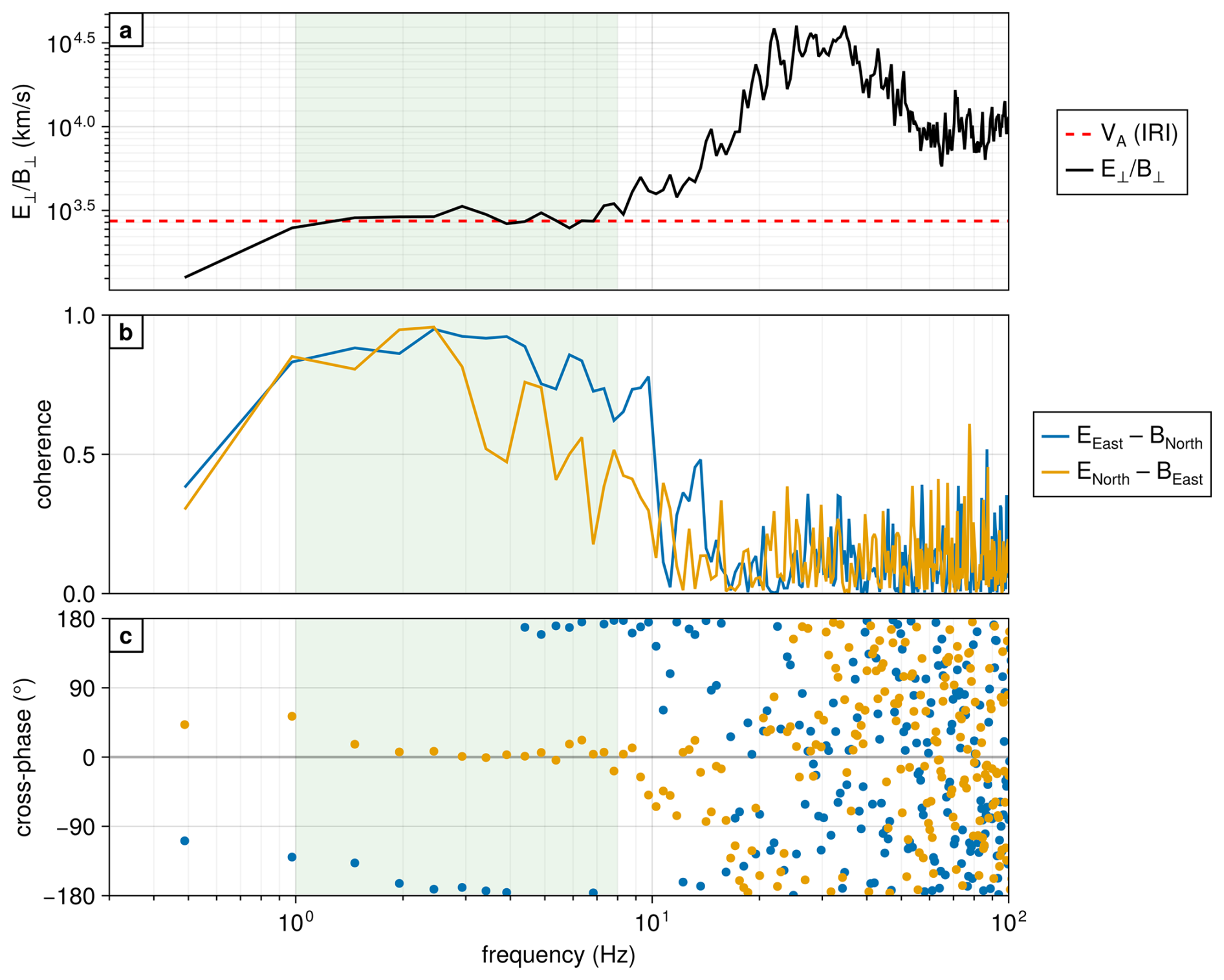
Figure A1 Cross-spectral analysis of the perpendicular fields over 331–340 s. (a) Ratio $E_{⟂}/B_{⟂}$ (black) and local MHD Alfvén speed V_A (red dashed). (b) Magnitude-squared coherence γ² for the two perpendicular-field pairings. (c) Cross-phase for the same pairings. The green band in all three panels marks the 1–8 Hz frequency range.

Table A1 Pitch-angle directions and widths of the channels of the low-flyer (35.040) EESA instrument.