Magnetosphere–ionosphere response to the 21 and 25 June 2015 coronal mass ejections

Using a coupled EUHFORIA–Gorgon-Space modelling chain, we simulate the magnetosphere–ionosphere coupled response to two coronal mass ejections (CMEs) that impacted Earth on 23 and 28 June 2015. The first CME (CME1), launched on 21 June, triggered a major geomagnetic storm (Kp = 8), driving strong magnetosphere–ionosphere coupling characterised by a cross-polar cap potential of 160 kV and intense field-aligned currents exceeding 23 MA, key indicators of energy transfer from the solar wind into the high-latitude ionosphere. In contrast, the faster CME2 (launched on 25 June) produced only a weak disturbance (Kp ≈ 2) due to the absence of a prolonged southward interplanetary magnetic field (IMF), resulting in minimal magnetospheric driving and ionospheric feedback. These results validate an end-to-end space-weather forecasting framework and demonstrate that CME geoeffectiveness is governed primarily by the IMF orientation and reconnection-driven magnetosphere–ionosphere energy coupling, rather than by kinematic properties such as speed alone.

1 Introduction

Coronal Mass Ejections (CMEs) are a primary driver of major geomagnetic storms and represent one of the most significant space-weather threats to technological systems (Gosling, 1993; Lyon, 2000). The severity of these storms is determined by the distinct properties of the CME-driven solar wind, which often exhibits a significantly enhanced charged-particle density and a strongly southward-oriented interplanetary magnetic field (IMF). The interaction of this structured plasma with Earth's magnetosphere does not merely cause compression; it also drives a large-scale transfer of energy and momentum. This forces the magnetosphere into a disturbed state and enables energetic particles to penetrate deeply, ultimately funnelling energy into the ionosphere and triggering a complex chain of electrodynamic phenomena (Moore et al., 1999).

The scientific community acknowledges the growing importance of space weather, given its effects on human activities. Predicting space weather phenomena requires modelling distinct plasma environments, from the solar corona to the Earth's magnetosphere, each dominated by different physical processes (e.g., magnetohydrodynamics, kinetic theory). To address this issue, the ESA Virtual Space Weather Modelling Centre (VSWMC) has enhanced its capabilities to incorporate multiple models to predict space weather (Poedts et al., 2020).

Transient structures in the solar wind, such as coronal mass ejections (CMEs) and corotating interaction regions, drive space-weather effects through their interactions with Earth's coupled magnetosphere–ionosphere system. These transients often carry interplanetary shocks at their leading edges and exhibit strong southward magnetic-field components. Shock impact causes a sudden increase in solar wind dynamic pressure, which rapidly compresses the dayside magnetopause and the entire magnetospheric cavity. This impulsive compression produces a characteristic ground magnetic signature, a sharp bipolar variation in the horizontal component, known as a Sudden Impulse (SI) (Smith et al., 2019). When the initial compression is followed by sustained energy input (typically via southward IMF-driven reconnection) and the development of a full geomagnetic storm, the event is specifically termed a Storm Sudden Commencement (SC) (Araki, 1994; Goldstein and Schindler, 1978). Both SIs and SCs pose significant hazards to power infrastructure, as their rapid magnetic field variations can induce extremely high geomagnetically induced currents (GICs) in long conductors (Eastwood et al., 2018).

Space weather, driven by solar activity such as Coronal Mass Ejections (CMEs), poses a significant risk to modern technological infrastructure. CMEs, which involve the violent expulsion of plasma and magnetic fields from the Sun, can trigger severe geomagnetic storms upon interaction with Earth's magnetosphere. The ionospheric response to CMEs can vary, depending on the properties of the CME and the geomagnetic conditions. The redistribution of ionospheric plasma during a geomagnetic storm can cause significant disruptions to radio communications. These disruptions can affect the reliability and quality of signal propagation through the ionosphere, thereby impacting various communication systems that rely on this medium (Kappenman, 2001; Astafyeva et al., 2014). High-frequency (HF) radio signals can be more strongly absorbed in the ionosphere during such disturbances, thereby affecting long-distance radio communications by altering the propagation path and velocity of radio waves (Priyadarshi et al., 2016; Hayes et al., 2017). Additionally, radio signals can experience greater signal fading and path fluctuations as they traverse the ionospheric regions (Araki, 1974). CME-induced ionospheric disturbances can also affect satellite-based navigation systems like GPS (Global Positioning System) (Demyanov et al., 2012). The radio signals from GPS satellites passing through the disturbed ionosphere may experience propagation delays and errors (Rama Rao et al., 2009). These delays can introduce inaccuracies in GPS position estimates, thereby affecting navigation and timing applications.

Furthermore, the super-magnetosonic solar wind flows past the magnetosphere, forming a bow shock. The ever-changing nature of the solar wind causes the magnetospheric boundaries to shift continuously in response to variations in dynamic pressure and the interplanetary magnetic field (IMF). The size and shape of the magnetospheric obstacle primarily determine the stand-off distance of the bow shock. Since the magnetopause's location is determined by the balance between solar wind dynamic pressure and Earth's magnetic pressure, the bow shock's position shows a clear dependence on solar wind conditions. Empirical models often parameterise the bow shock based on this relationship (Merka et al., 2005; Peredo et al., 1995), building on the foundational gasdynamic principles established by Spreiter et al. (1966).

Beyond usual solar wind fluctuations, the most rapid and substantial movements of magnetospheric boundaries are caused by distinct transient structures, particularly interplanetary shocks (Dryer et al., 1967; Grib et al., 1979). Numerical simulations and spacecraft observations have consistently shown that the impact of an interplanetary shock on the magnetosphere leads to a global, rapid compression. For instance, simulations by Samsonov et al. (2007) demonstrate significant inward motion of the bow shock and magnetopause upon the shock's arrival. This compression directly drives ground-level phenomena such as Sudden Commencements (SCs). Intriguingly, these model results are strongly supported by in-situ spacecraft measurements (Pallocchia, 2013).

In general, empirical models have limitations in capturing the motion of shocks that arise in response to rapid changes in the upstream solar wind. Specifically, there is limited understanding of when these statistical models become unsuitable, and it is unclear how they deviate from reality during the dynamic transition of boundaries toward new equilibrium states. To overcome these limitations, the space science community has long employed global magnetohydrodynamic (MHD) simulations, a powerful tool for modelling the coupled system in a self-consistent manner. Since their development in the 1990s (e.g., Ogino, 1994; Raeder, 1995), global MHD models have been extensively used to study magnetospheric dynamics. Today, a suite of well-established models (e.g., the LFM code, the OpenGGCM, SWMF/BATS-R-US) continues to advance our understanding. Within this modelling paradigm, our study employs the Gorgon code to conduct global MHD simulations of Earth's magnetosphere under dynamic solar wind conditions (Chittenden et al., 2004; Ciardi et al., 2007; Mejnertsen et al., 2016).

While empirical models provide valuable statistical representations of magnetospheric boundaries, they are inherently limited in capturing the rapid, non-equilibrium dynamics driven by transient solar wind structures, such as CME-driven shocks. These models struggle to accurately represent the motion of shocks and the transient reconfiguration of boundaries, such as the bow shock and magnetopause, during their dynamic transition to new equilibrium states. To overcome these limitations, this study employs the Gorgon-Space code, a global magnetohydrodynamic (MHD) model. The primary aim of using Gorgon-Space is to conduct high-fidelity, time-dependent simulations of Earth's magnetosphere-ionosphere system in response to realistic, time-varying solar wind input. This approach allows us to accurately capture the full system's consistent and coupled response, including magnetospheric compression, the activation of current systems, and the subsequent ionospheric electrodynamic feedback, thereby providing a physically consistent framework to investigate the geospace environment's response to specific CME events (Chittenden et al., 2004; Ciardi et al., 2007; Mejnertsen et al., 2016).

The coupling among the solar wind, magnetosphere, and ionosphere, mediated by field-aligned currents (FACs), is a fundamental driver of space-weather phenomena. Accurate global MHD modelling of this coupled system is therefore essential for prediction (e.g., Pulkkinen, 2007; Gombosi et al., 2021).

Significant progress has been made in simulating large-scale magnetospheric dynamics and their ionospheric signatures. Models such as the Space Weather Modelling Framework (SWMF) and the Gorgon-Space code have demonstrated skill in reproducing global convection patterns and regional FAC distributions during specific events (e.g.,Wiltberger et al., 2017; Sorathia et al., 2023). These models solve the coupled MHD magnetosphere-ionosphere system, in which ionospheric conductances, critical for determining the electric field mapped to the magnetosphere, are often derived from empirical relations.

The remaining challenge, however, lies in accurately reproducing electric fields and current densities in key regions, such as the plasma sheet, during dynamic solar wind driving. Discrepancies between modelled and observed fields in these regions can propagate, affecting the entire system's response and impacting the fidelity of space weather forecasts. This study specifically addresses this challenge by evaluating the performance of the Gorgon-Space code in simulating FACs and associated electric fields. We focus on the role of the inner boundary definition and the empirical conductance models in determining the accuracy of the coupled solution.

In the Gorgon-Space code, the ionosphere is treated as a two-dimensional spherical shell at approximately 1 R_E (Earth radius) from the Earth's centre. This boundary is characterised by a height-integrated conductance model (typically including both Pedersen and Hall conductances), which may be specified as empirical values or calculated self-consistently based on precipitation patterns. The magnetosphere-ionosphere coupling is enforced by mapping field-aligned currents (FACs), calculated from the magnetospheric vorticity in the simulation, down to this ionospheric shell. The ionospheric solver then computes the resulting electric potentials and currents, which, in turn, influence the magnetospheric flow via boundary conditions on the magnetic field and plasma, thereby closing the coupled system.

The upstream (sunward) boundary of the simulation is driven by time-dependent solar wind parameters obtained from the EUHFORIA (European Heliospheric Forecasting Information Asset) model. These parameters, which include number density, velocity, thermal pressure, and the interplanetary magnetic field (IMF) components, provide the external forcing for the magnetospheric simulation.

The dynamic and non-uniform nature of Earth's magnetosphere presents a substantial modelling challenge, as a complex interplay between the solar wind, internal magnetic field, and various plasma populations determines its global state. A comprehensive understanding requires modelling the magnetosphere and ionosphere as a tightly coupled system in which energy and momentum are transferred along magnetic field lines. This magnetosphere-ionosphere (M-I) coupling is primarily mediated by Field-Aligned Currents (FACs), which are intrinsically linked to vorticity and pressure gradients in the magnetospheric plasma. The Gorgon-Space code is uniquely well-suited to model this coupled system, as it solves the global MHD equations to self-consistently simulate the vast magnetospheric domain while simultaneously capturing FAC generation and their closure in the ionosphere. Consequently, this study utilises Gorgon-Space to investigate the transient variations in FACs and ionospheric potentials driven by CME impacts, providing a physics-based assessment of the dynamic M-I system's response to extreme space weather events.

This study applies the established end-to-end modelling approach, linking heliospheric and magnetospheric codes, to the specific case of interacting CMEs in June 2015, using the EUHFORIA–Gorgon-Space coupling. Gorgon-Space was selected for this work due to its unique formulation based on the magnetic vector potential, which inherently preserves $\mathrm{\nabla }\cdot \mathit{B}=\mathrm{0}$ to machine precision. This property is critical for maintaining numerical stability during extreme, rapidly varying compression events, such as CME impacts, where spurious magnetic monopoles in standard B-field solvers can degrade solution fidelity. Furthermore, Gorgon-Space has been rigorously validated for simulating field-aligned currents (FACs) and ionosphere-magnetosphere coupling during storm-time conditions (Mejnertsen et al., 2018; Eggington et al., 2020). Leveraging these strengths, we conduct a comparative analysis of two CME events and successfully capture intense geoeffective signatures, including FACs exceeding 23 million amperes and a cross-polar cap potential of ∼160 kV for CME1, while correctly reproducing the muted response to CME2. These results demonstrate Gorgon-Space’s capability to forecast key magnetospheric drivers of space weather impacts, providing a validated, physics-based methodology for translating heliospheric CME forecasts into quantifiable geospace impact predictions.

The objective of our study is to investigate the interaction between two CMEs and Earth and their effects on Earth's ionosphere and magnetosphere. In this research, we utilise Gorgon-Space to explore how Earth's magnetosphere responds to interactions with CMEs and to study the impact of CMEs on the magnetosphere. In conclusion, the study examines how the ionosphere reacts to the interaction between CMEs and the magnetosphere. It also evaluates the consequential effects on the ionosphere, including induced current densities, which significantly affect communication and space weather.

2 Method

2.1 EUHFORIA Heliospheric Model

The European Heliospheric Forecasting Information Asset (EUHFORIA) is a three-dimensional magnetohydrodynamic (MHD) model of the inner heliosphere that simulates the propagation of solar wind structures from the Sun to 2 AU (Pomoell and Poedts, 2018; Rodgers-Lee et al., 2021). The model domain extends from a spherical inner boundary at 0.1 AU to an outer boundary at 2.0 AU, with spatial resolution increasing with heliocentric distance. EUHFORIA solves the ideal MHD equations for a fully ionised plasma under the influence of solar gravity and the interplanetary magnetic field.

Coronal Mass Ejections are injected at the inner boundary as time-dependent, flux-rope structures characterised by their launch time, location (longitude/latitude), angular width, and initial speed. The model self-consistently propagates these transients through the ambient solar wind, capturing CME–CME and CME–solar wind interactions, shock formation, and magnetic field evolution en route to Earth.

At the L1 Lagrange point (approximately 1.5 million km sunward of Earth), EUHFORIA provides time series of key solar wind parameters: proton number density n_p (cm⁻³), bulk velocity V (km s⁻¹), thermal pressure P_th (nPa), and the three components of the interplanetary magnetic field B (nT) in GSE coordinates. These parameters serve as the direct upstream boundary conditions for global magnetospheric models such as Gorgon-Space.

EUHFORIA's ambient solar wind predictions have been extensively validated against OMNI observations in previous studies (Pomoell and Poedts, 2018; Scolini et al., 2020), and the present study focuses on the subsequent magnetospheric-ionospheric response using these EUHFORIA outputs as input to Gorgon-Space.

2.2 Gorgon-Space Model

Gorgon is a 3D magnetohydrodynamic code, originally developed to study high-energy, collisional plasma interactions, such as Z-pinches (Chittenden et al., 2004; Jennings et al., 2010), laser-plasma interactions (Smith et al., 2007), and magnetic tower jets (Ciardi et al., 2007). It has recently been adapted to simulate planetary magnetospheres and their interaction with the solar wind (Mejnertsen et al., 2016). The code solves the resistive MHD equations using a semiconservative formulation. In this approach, the equations for mass, momentum, and energy are solved in a fully conservative form, which ensures accurate capture of shocks and discontinuities. The magnetic field, however, is evolved using the induction equation (a non-conservative form), typically coupled with a divergence-cleaning technique to maintain the solenoidal constraint ($\mathrm{\nabla }\cdot \mathit{B}=\mathrm{0}$). Most of its primary features are designed for intricate collisional and resistive Magnetohydrodynamics (MHD) phenomena (Ciardi et al., 2007).

Gorgon-Space has been created specifically to tackle the challenge of conducting global magnetospheric simulations for space weather and space physics. Therefore, it currently represents a distinct area of enhancement and has been optimised and evaluated for particular use cases. A key feature of Gorgon-Space is that it evolves the magnetic vector potential (A) instead of the magnetic field (B) directly. This approach, also used in other models (e.g., Yagi et al., 2009), inherently guarantees that the magnetic field remains divergence-free (i.e., $\mathrm{\nabla }\cdot \mathit{B}=\mathrm{0}$) by construction, which is a significant numerical advantage (Mejnertsen et al., 2018; Eggington et al., 2020).

Gorgon-Space utilises a definite-sized 3D Cartesian grid to solve the MHD equations. Moreover, Gorgon possesses a highly advanced capability to scale linearly and in parallel across numerous cores, using fully explicit numerical methods. It found the impact of the solar wind on several important parameters in the tail, including the magnetic field, field-aligned current, plasma velocity, and plasma pressure. These global quantities depend on the magnetosphere's large-scale equilibrium, which is believed to be accurately described by magnetohydrodynamics (MHD).

Gorgon uses a fully explicit Eulerian formulation of the resistive semiconservative MHD equations for a fully ionised plasma as

$$\begin{array}{}\text{(1)}& {\displaystyle \frac{\partial \mathit{\rho }}{\partial t}}+\mathrm{\nabla }\cdot \left(\mathit{\rho }\mathit{V}\right)=\mathrm{0},\text{(2)}& {\displaystyle }\begin{array}{rl}\mathit{\rho }\left[{\displaystyle \frac{\partial \mathit{V}}{\partial t}}+(\mathit{V}\cdot \mathrm{\nabla })\mathit{V}\right]& =\left({\displaystyle \frac{\mathrm{1}}{\mathit{\mu }}}\mathrm{\nabla }\times \mathit{B}\right)\times \mathit{B}\\ & -\mathrm{\nabla }(P_{\mathrm{e}}+P_{\mathrm{p}}),\end{array}\text{(3)}& {\displaystyle \frac{\partial \mathit{B}}{\partial t}}=\mathrm{\nabla }\times (\mathit{V}\times \mathit{B})+\mathit{\eta }{\mathrm{\nabla }}^{\mathrm{2}}\mathit{B},\text{(4)}& {\displaystyle \frac{\partial {\mathit{ϵ}}_{\mathrm{p}}}{\partial t}}+\mathrm{\nabla }\cdot \left({\mathit{ϵ}}_{\mathrm{p}}\mathit{V}\right)=-P_{\mathrm{p}}\mathrm{\nabla }\cdot \left(\mathit{V}\right)-{\mathrm{\Delta }}_{\mathrm{pe}},\text{(5)}& {\displaystyle \frac{\partial {\mathit{ϵ}}_{\mathrm{e}}}{\partial t}}+\mathrm{\nabla }\cdot \left({\mathit{ϵ}}_{\mathrm{e}}\mathit{V}\right)=-P_{\mathrm{e}}\mathrm{\nabla }\cdot \left(\mathit{V}\right)+{\mathrm{\Delta }}_{\mathrm{pe}}-\mathrm{\Lambda }+\mathit{\eta }\left|{\mathbf{J}}^{\mathrm{2}}\right|,\end{array}$$

The plasma density, plasma velocity, magnetic field, proton internal energy density, electron internal energy density and thermal pressure are represented by the variables ρ, V, B ϵ_p, ϵ_e, and P respectively. The values μ, η, and $\mathit{\gamma }=\mathrm{5}/\mathrm{3}$ represent the magnetic permeability, the magnetic diffusivity, and the ratio of specific heats at constant pressure and volume, respectively. The permeability of vacuum is considered i.e. $\mathit{\mu }=\mathrm{4}\mathit{\pi }\times {\mathrm{10}}^{-\mathrm{7}}$ Hm⁻¹. The deBar correction, known as Von Neumann artificial viscosity, is utilised to accurately detect and enhance energy conservation in the presence of shocks (Benson, 1992). Gorgon makes use of second-order Van Leer advection to solve the advection terms in equations. It also employs a variable time step, which automatically satisfies the relevant Courant conditions.

The MHD formulation in Gorgon has its roots in high-energy-density plasma physics, leading to several features that are atypical of global magnetospheric simulations. A key aspect is that it solves separate internal energy equations for electrons and protons, allowing them to be out of thermodynamic equilibrium. The electron energy equation includes physically important terms.

Ohmic Heating ($\mathit{\eta }\left|{\mathbf{J}}^{\mathrm{2}}\right|$), where the resistivity η is treated as a constant value or a Spitzer-like model dependent on local electron temperature (Jennings et al., 2010). Electron-Proton Energy Exchange (Δ_pe), which is modelled as a collisional relaxation term of the form ${\mathrm{\Delta }}_{\mathrm{pe}}={\mathit{\nu }}_{\mathrm{ep}}nk(T_{\mathrm{p}}-T_{\mathrm{e}})$, driving the two populations towards thermal equilibrium (Chittenden et al., 2004). Given the tenuous plasma conditions in the magnetosphere, the optically thin radiation loss term (Λ) is neglected in the present study (Λ=0) because radiative cooling is negligible relative to other energy transport mechanisms.

Furthermore, the code evolves internal energy rather than total energy. While this means total energy is not strictly conserved, it is a deliberate design choice that significantly enhances numerical robustness. This approach effectively mitigates the occurrence of non-physical negative pressures in regions of high magnetic energy or strong shocks, which is a common numerical challenge in conservative total-energy schemes.

The Gorgon-Space code solves separate internal energy equations for electrons and protons. Therefore, the total thermal pressure provided by EUHFORIA must be partitioned at the boundary. For this study, we assume the proton and electron populations are in thermal equilibrium (T_p=T_e) upon entry, resulting in an equal split of the pressure ($P_{\mathrm{p}}=P_{\mathrm{e}}=P_{\mathrm{tot}}/\mathrm{2}$). The upstream (sunward) boundary of the simulation is driven by time-dependent solar wind parameters obtained from the EUHFORIA heliospheric model.

The treatment of the inner boundary of the magnetospheric domain in Gorgon is similar to that used in other codes, which are coupled to a thin-shell ionosphere model. The approach is to define the plasma density, temperature, and velocity throughout the spherical region enclosed by the inner boundary and enforce them at every time step. The cells for which this is performed are flagged as inner boundary cells if the cell centre lies within the specified inner boundary radius RIB, typically set to 4 R_E (Earth radius). Whilst the MHD equations are not solved in this region, the cells just outside of the boundary are updated based on the inner boundary properties. Thus, the cold, dense plasma expands to form a plasmasphere, and the inner boundary flow feeds into the global magnetosphere.

The grid namelist specifies the domain size and resolution, as well as the dimensional splitting for parallelisation. The default box has dimensions $\mathrm{90}\times \mathrm{80}\times \mathrm{80}$ R_E and spans $(X,Y,Z)=\left(\right[-\mathrm{24},\mathrm{66}],[-\mathrm{40},\mathrm{40}],[-\mathrm{40},\mathrm{40}\left]\right)$ R_E, and should be kept as close as possible to these dimensions to balance runtime and stability. The simulation utilizes a fixed computational grid with a resolution of 0.5 R_E to resolve the global structure of the magnetosphere. This resolution was chosen to accurately capture large-scale boundaries and dynamics, such as the positions of the bow shock and magnetopause, and the overall evolution of the magnetotail, while remaining computationally tractable for the extended simulation runs required for this study. The grid dimensions are $(n_x,n_y,n_z)=(\mathrm{180},\mathrm{160},\mathrm{160})$ cells, which defines the 0.5 R_E grid spacing throughout the domain.

The simulation utilises a fixed computational grid within a Cartesian domain spanning from $(X,Y,Z)=\left(\right[-\mathrm{24},\mathrm{66}],[-\mathrm{40},\mathrm{40}],[-\mathrm{40},\mathrm{40}\left]\right)$ R_E. This domain size encompasses the critical regions from the dayside bow shock to a significant portion of the magnetotail. The grid consists of $(n_x,n_y,n_z)=(\mathrm{180},\mathrm{160},\mathrm{160})$ cells, resulting in a uniform resolution of 0.5 R_E. This resolution was chosen to accurately capture large-scale boundaries and dynamics, such as the positions of the bow shock and magnetopause and the general evolution of the magnetotail, while maintaining computational tractability for the parameter study.

3 Numerical results and discussion

We selected two CMEs from the June 2015 campaign that exhibited contrasting geoeffectiveness despite both being fast events:

• CME1: Launched on 21 June 2015 at 05:01 UT from heliographic coordinates (longitude $=-\mathrm{8}$°, latitude $=+\mathrm{7}$°) with an initial speed of 1250 km s⁻¹ (Table 1). EUHFORIA predicted its arrival at Earth on 23 June 2015 at 00:03 UT, where it triggered a major geomagnetic storm (peak Kp = 8).

• CME2: Launched on 25 June 2015 at 10:51 UT (longitude $=+\mathrm{46}$°, latitude $=+\mathrm{23}$°) with a higher initial speed of 1450 km s⁻¹. EUHFORIA predicted its arrival on 28 June 2015 at 12:52 UT, but it produced only a minor disturbance (peak Kp ≈2).

This pair provides an ideal test case to isolate the role of IMF orientation versus CME kinematics in determining geoeffectiveness.

Table 1 List of CMEs observed during 10–25 June 2015 and injected into EUHFORIA. Events marked with ^a (21 June) and ^b (25 June) correspond to CME1 and CME2, respectively, the two events selected for detailed magnetospheric simulation with Gorgon-Space due to their contrasting geoeffectiveness.

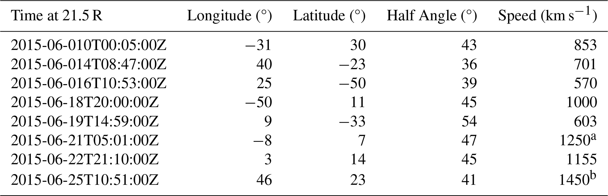
According to Table 1, while CME2 exhibited higher kinematic speed (1450 vs. 1250 km s⁻¹ for CME1), its geoeffectiveness was minimal due to the absence of sustained southward IMF ($B_z>-\mathrm{5}$ nT for >90 % of the event duration as it is shown in Fig. 1). This contrasts sharply with CME1, which maintained $B_z<-\mathrm{15}$ nT for >6 h, driving intense dayside reconnection (E_y>15 mV m⁻¹) and producing the observed G4 storm (Kp = 8, Dst $\approx -\mathrm{200}$ nT). These results definitively demonstrate that CME speed alone is insufficient to predict storm intensity – the orientation of the embedded magnetic field governs geoeffectiveness.

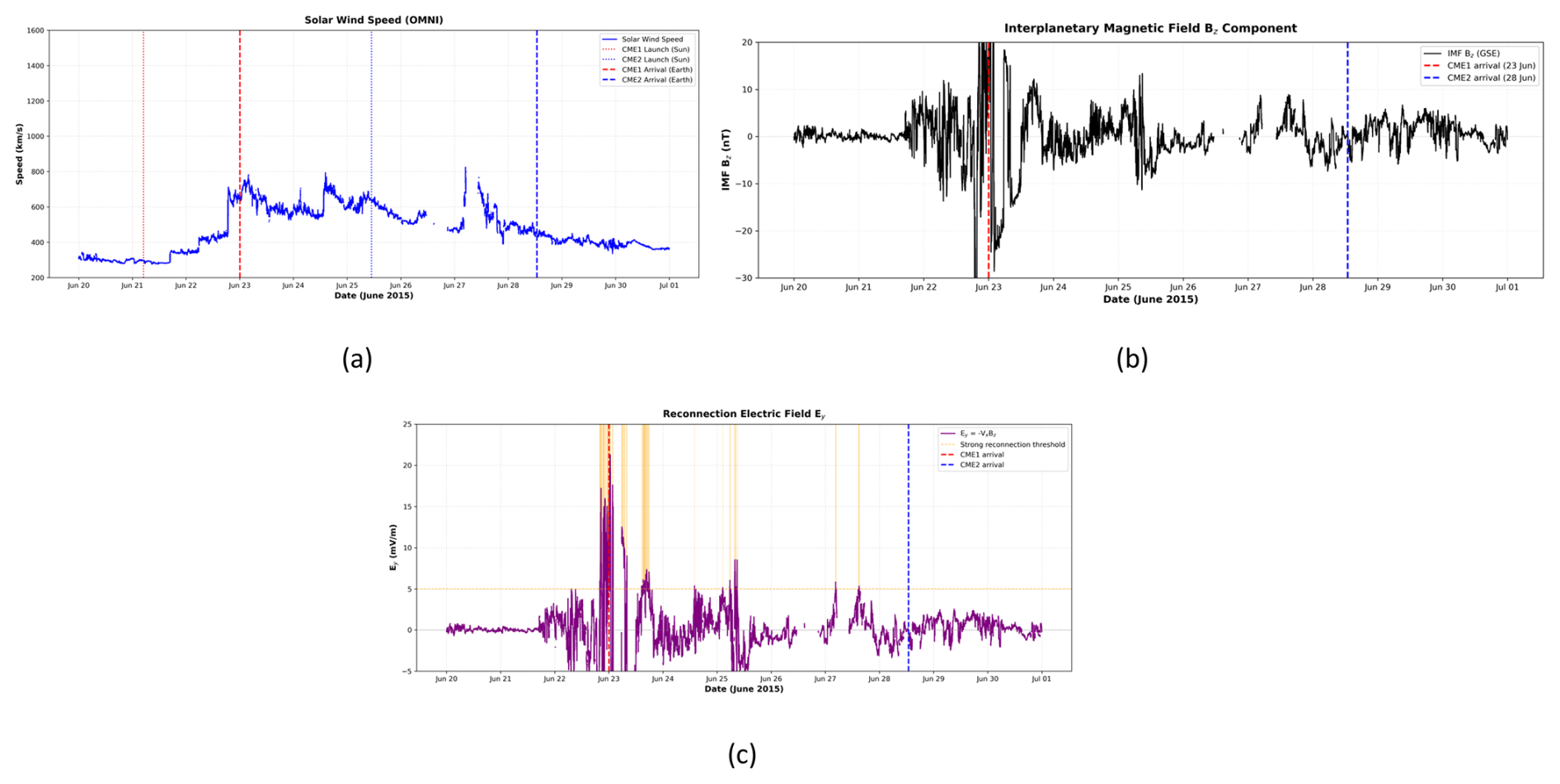
Figure 1 Solar wind and IMF conditions during June 2015. (a) Solar wind speed showing CME1 and CME2 launch times (at the Sun) and arrival times (at Earth). (b) IMF B_z component with southward excursions highlighted. (c) Reconnection electric field $E_y=-V_x{B}_z$. Vertical dashed lines mark CME1 arrival (23 June) and CME2 arrival (28 June). CME1 exhibits sustained southward B_z ($<-\mathrm{15}$ nT) and strong E_y (>15 mV m⁻¹), driving intense magnetospheric activity. CME2 shows only weak southward B_z and minimal E_y despite comparable speed, resulting in negligible geoeffectiveness.

The transfer of energy from the solar wind into the Earth's magnetosphere-ionosphere system during geomagnetic storms is primarily governed by dayside magnetic reconnection, a process whose efficiency is controlled by the orientation and magnitude of the interplanetary magnetic field (IMF) and the solar wind speed. The southward component of the IMF (B_z<0 in GSM coordinates) enables the solar wind magnetic field to reconnect antiparallel to Earth's northward-directed dayside field, thereby opening previously closed magnetospheric field lines and allowing solar wind momentum and energy to enter the system. The reconnection electric field, defined as $E_y=-V_x\times B_z$, is a widely accepted proxy for the rate of energy transfer (e.g., Dungey, 1961; Gonzalez et al., 1994).

Figure 1 presents OMNI solar wind and IMF data for June 2015, quantifying the key drivers of the two CME events. Panel (a) shows the solar wind speed, with vertical dashed lines marking the launch times (at the Sun) and arrival times (at Earth) for CME1 and CME2. Both CMEs produced significant speed enhancements: CME1 reached approximately 790 km s⁻¹ upon arrival on 23 June, while CME2 reached approximately 680 km s⁻¹ on 28 June.

Panel (b) displays the IMF B_z component. CME1 is characterised by an intense and sustained southward IMF ($B_z<-\mathrm{15}$ nT) that persists for several hours following its arrival. In contrast, CME2 exhibits only brief, weak southward IMF excursions ($B_z>-\mathrm{5}$ nT for most of the event), despite its comparable speed.

Panel (c) shows the reconnection electric field $E_y=-V_x{B}_z$. CME1 drives a large reconnection electric field exceeding 15 mV m⁻¹, indicative of vigorous dayside reconnection. CME2 produces a correspondingly low E_y (< 3 mV m⁻¹) due to the absence of sustained southward B_z.

Thus, Fig. 1 provides the causal link between interplanetary conditions and the divergent magnetospheric-ionospheric responses to the two CMEs. It confirms that CME speed alone is insufficient to predict storm intensity; rather, the IMF B_z orientation and the resulting reconnection-driven energy coupling are the dominant factors. This observation validates a core principle of space-weather physics and underscores the importance of accurate IMF forecasting for predicting geomagnetic impacts.

Geomagnetic activity indices provide complementary diagnostics for characterising the intensity and physical drivers of space weather events. The Kp index (planetary K-index) quantifies global auroral-zone magnetic disturbances on a quasi-logarithmic scale from 0–9, derived from 3-hourly measurements at 13 mid-latitude magnetometers (Bartels and Veldkamp, 1949). While Kp is operationally valuable for space-weather alerts because of its sensitivity to high-latitude currents, it does not directly measure the ring current responsible for main-phase storm development.

For definitive storm classification, the Dst (Disturbance Storm Time) index (Sugiura, 1964) and its 1 min resolution counterpart SYM-H (Iyemori, 1990) are the standard metrics. These indices, derived from low-latitude magnetometer networks, measure the depression of the horizontal magnetic field component caused by the symmetric ring current encircling Earth. By convention (Gonzalez et al., 1994), a geomagnetic storm is defined when Dst/SYM-H <−50 nT, with categories of moderate (−50>Dst≥−100 nT), intense (−100>Dst≥−250 nT), and super-intense (Dst<−250 nT) storms. Unlike Kp, Dst/SYM-H directly reflects energy injection into the inner magnetosphere and is therefore the authoritative metric for assessing storm intensity.

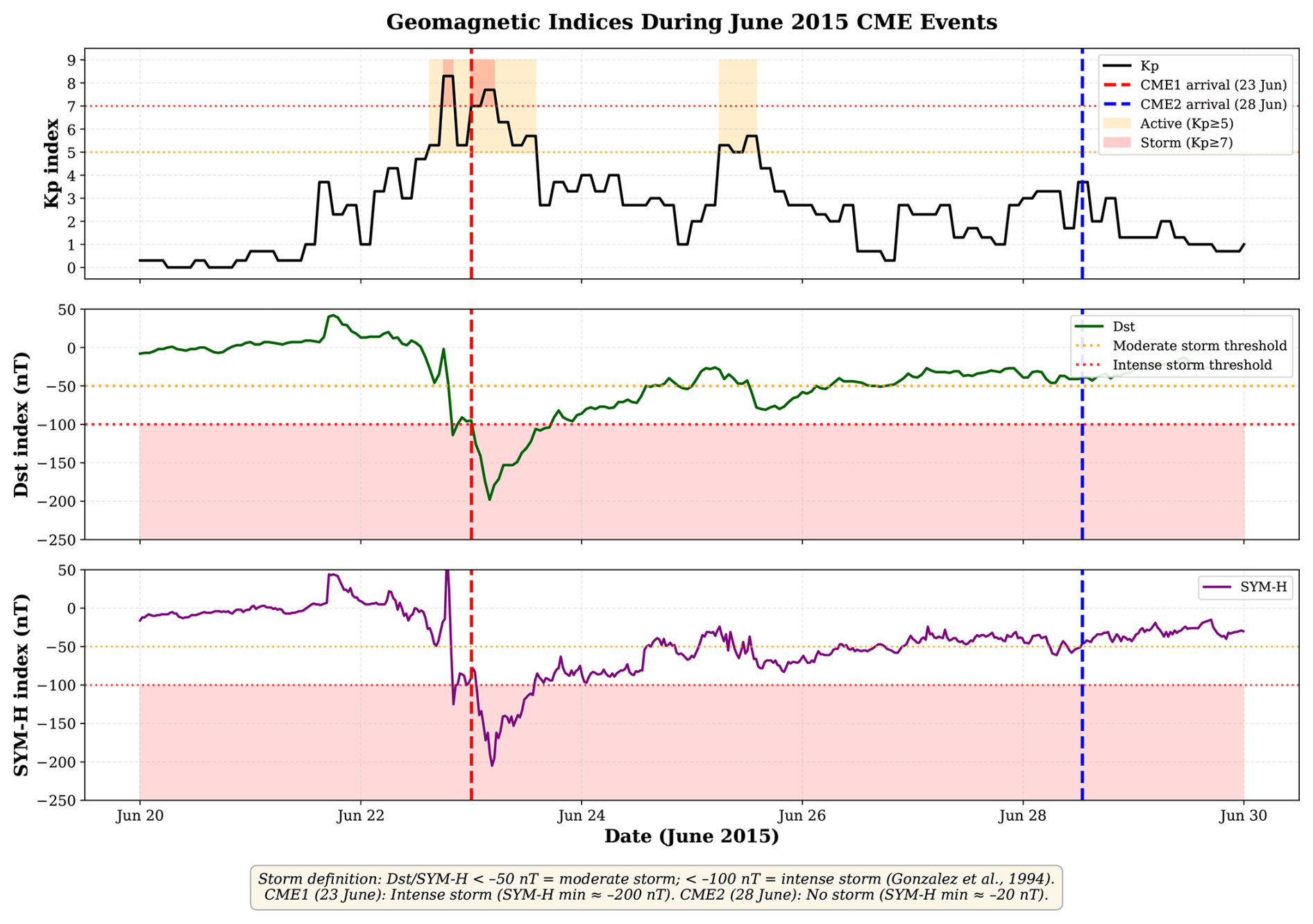
Figure 2 Geomagnetic response to CME1 (23 June 2015) and CME2 (28 June 2015) impacts. Top to bottom: Kp index, Dst index, and SYM-H index. Vertical dashed lines mark EUHFORIA-predicted CME arrival times at L1. Storm intensity thresholds are indicated by horizontal lines: orange (−50 nT, moderate storm) and red (−100 nT, intense storm) per Gonzalez et al. (1994). CME1 produced an intense geomagnetic storm with SYM-H minimum ≈−200 nT, while CME2 showed only a minor disturbance (SYM-H minimum ≈−20 nT) despite a brief Kp elevation. This demonstrates that high Kp values alone do not constitute a magnetic storm; Dst/SYM-H quantifies the development of the ring current that defines storm intensity.

Dst and SYM-H values shown in Fig. 2 are observational data from the OMNI databases, used here solely for event classification and validation of the simulated magnetospheric response, not as model outputs. These indices objectively confirm that CME1 (23 June 2015) produced an intense geomagnetic storm (SYM-H minimum ≈−200 nT), while CME2 (28 June 2015) generated only a minor disturbance (SYM-H minimum ≈−20 nT) despite a brief Kp elevation during its shock arrival.

While Sabri and Poedts (2025) established the fidelity of EUHFORIA's heliospheric forecasts and their conversion to geomagnetic activity estimates, the present work focuses on the next critical step in the space weather chain: translating EUHFORIA's time-dependent solar wind parameters (density, velocity, IMF) at L1 into a self-consistent simulation of the coupled magnetosphere–ionosphere response using Gorgon-Space. We do not aim to improve Kp/Dst forecasting algorithms; rather, we leverage these indices solely to classify the two contrasting events (major storm vs. weak disturbance) and then investigate, through first-principles MHD simulation, the underlying plasma processes (magnetospheric compression, FAC intensification, convection electric fields) that produce these differing geomagnetic signatures. This end-to-end approach bridges heliospheric prediction and geospace impact quantification, providing a physics-based framework for operational space-weather forecasting.

A systematic study was conducted to demonstrate the global fluctuations in the magnetic field using magnetic observations. These differences were credited to the influence of solar wind discontinuities on both the Earth's magnetosphere and ionosphere. Magnetic reconnection is the primary process through which plasma and energy from the solar wind are introduced into the magnetosphere. However, there are also cases where viscous-like effects can play a role, especially when the magnetic setup is unsuitable for reconnection. In this part, we examine how the arrival of CMEs affects Earth. The Gorgon-Space code is utilised in this specific situation.

When the solar wind interacts with the Earth's magnetosphere, it generates a bow shock wave that forms ahead of the magnetopause. This results in the formation of a turbulent region, known as the magnetosheath, situated between them, a structure first described in the seminal work of Spreiter et al. (1966) and studied in its turbulent nature by Lucek et al. (2005) and Burgess and Scholer (2013). To enable plasma to move away from the planet, for example, when the solar wind is redirected around the magnetopause or when magnetospheric plasma is expelled towards the tail, it is necessary to implement free-flow at the outer boundaries of the simulation domain. One exception to this rule occurs on the side of the box facing the Sun, specifically on Earth's left side. This is where the simulation receives and relies on the solar wind inflow to serve as the main source of plasma.

The key input to the simulation is the time-dependent solar wind plasma, whose parameters are specified at this boundary. These parameters, derived from the EUHFORIA heliospheric model, illustrate variations in the solar wind that directly control the formation and properties of the bow shock. On the remaining outer boundaries (tailward, lateral, and polar), free-flow (outflow) conditions are implemented. This configuration allows plasma to exit the domain, whether it is solar wind being deflected around the magnetosphere or magnetospheric plasma being ejected downtail, without generating unphysical reflections, a standard approach in global magnetospheric simulations (Spreiter et al., 1966; Lucek et al., 2005; Burgess and Scholer, 2013).

Gorgon-Space was selected for this study due to its divergence-free magnetic field formulation (via vector potential evolution), which ensures numerical stability during extreme compression events, and its validated performance in simulating FACs and ionospheric coupling during CME impacts (Mejnertsen et al., 2018; Eggington et al., 2020).

All simulation results and figures in this study are presented in the Geocentric Solar Ecliptic (GSE) coordinate system. In GSE:

• The x axis points from Earth toward the Sun.

• The y axis points opposite to Earth's orbital motion (i.e., duskward).

• The z axis completes the right-handed system, pointing northward perpendicular to the ecliptic plane.

This differs from the Geocentric Solar Magnetospheric (GSM) coordinate system commonly used in magnetosphere-ionosphere coupling studies. In GSM, the x axis also points toward the Sun, but the y axis is defined to be perpendicular to both the x axis and the dipole axis, and the z axis is aligned with the dipole. Consequently, the directions of the x and y axes in our figures are opposite to those in GSM. The physics is coordinate-independent, and all interpretations remain valid.

3.1 Magnetospheric Response

The magnetosphere is influenced by interactions with the solar wind, which can be either viscous or pressure-driven, as described by Newell et al. (2008). The physical mechanisms that allow plasma and energy to flow from the solar wind into the magnetosphere are reconnection (Dryer, 1994) and viscous interaction (Axford and Hines, 1961). Dayside magnetic reconnection opens Earth’s closed field lines, enabling direct entry of solar wind plasma and momentum into the magnetosphere via magnetic flux transport. The solar wind conditions driving this simulation are the direct output from the EUHFORIA heliospheric model at the Earth's location (L1 point). This provides a physically consistent, time-dependent input boundary condition for the Gorgon-Space model, linking the CME's interplanetary propagation to its geoeffective impact.

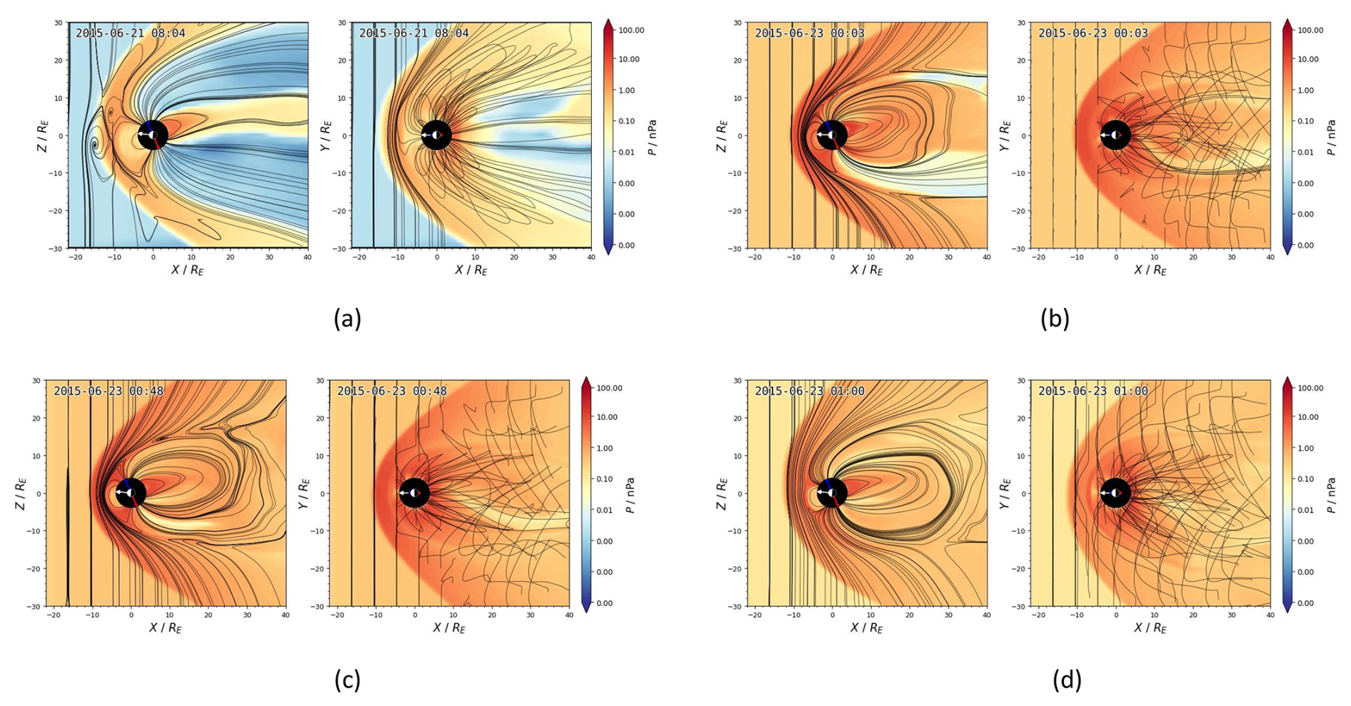
Figure 3 Snapshot of thermal pressure from the MHD simulation with Gorgon-Space. It depicts the arrival time of the first CME, which began on 21 June 2015 at 08:02 and reached Earth on 23 June 2015 at 00:03 UT, in the noon-midnight plane. All panels are shown in GSE coordinates.

The pronounced tailward stretching and distortion of the magnetotail observed in the XY plane during the CME1 impact (Fig. 3c–d) are consistent with the onset of magnetic reconnection in the magnetotail. Under enhanced solar wind dynamic pressure and southward IMF conditions (often associated with strong CMEs), reconnection in the near-Earth plasma sheet can lead to the formation of X-lines and the ejection of plasmoids, resulting in the observed elongation and structural deformation of the tail (e.g., (Baker et al., 1996; Hesse et al., 2004; Angelopoulos et al., 2008)). This process efficiently converts magnetic energy into kinetic and thermal energy, contributing to the global restructuring of the magnetosphere during geomagnetic storms. While reconnection also occurs at the dayside magnetopause, the tail configuration shown here is particularly indicative of nightside reconnection dynamics triggered by the intense solar wind forcing.

Figure 3 illustrates the evolution of thermal pressure and magnetic field topology during the arrival of CME1, as simulated by our global MHD model. The black lines represent magnetic field lines traced from seed points on a spherical surface at r=1 R_E, covering latitudes from −80 to +80° and longitudes spaced 15° apart. Field lines are numerically integrated along the magnetic field vector until they either close within the magnetosphere (connecting back to the opposite hemisphere) or extend beyond the magnetopause into the solar wind (defined as open if they reach x>10 R_E in the tail). The use of both x–z (noon–midnight meridian) and x–y (equatorial) planes allows us to reconstruct the magnetosphere's three-dimensional response to CME1, revealing dayside compression, tail stretching, and topological signatures of magnetic reconnection.

Panel (a) depicts the magnetospheric state approximately 2 d before CME1 arrival, corresponding to the time of the CME's initiation at the Sun (21 June 2015, 08:04 UT). While this snapshot provides context for the initial solar event, it does not represent the magnetospheric configuration immediately preceding the CME's impact at Earth. Panel (b), captured at 00:03 UT on 23 June 2015, depicts the magnetosphere at the time of CME1 arrival, showing significant dayside compression and elevated thermal pressure throughout the magnetosphere, particularly in the equatorial plane (x–y). This pressure enhancement coincides with a dramatic reconfiguration of the magnetic topology, most notably, the pronounced tailward stretching and distortion of the magnetotail observed in the x–y plane (panels c–d).

In Fig. 3, reconnection sites are inferred from topological changes in field line connectivity and localised enhancements in thermal pressure gradients. During this event, the solar wind reconnection electric field $E_y=-V_x{B}_z$ reached +18 mV m⁻¹ (see Fig. 1), well above the nominal 1–2 mV m⁻¹ threshold for strong magnetospheric driving. This large positive E_y implies a substantial southward (B_z<0) IMF component. Dayside reconnection is therefore inferred near the subsolar magnetopause, around (x≈10–12 R_E, z≈0) in the x–z plane, where closed field lines abruptly transition to open ones. Nightside reconnection is inferred in the near-Earth plasma sheet of the magnetotail, approximately at ($x\approx -\mathrm{20}$ to −25 R_E, y≈0) in the x–y plane, where the stretched tail field lines exhibit a sharp reversal in direction and enhanced pressure, consistent with the formation of a neutral X-line and plasmoid ejection.

This tail deformation is consistent with the onset of magnetic reconnection in the near-Earth plasma sheet. Under the enhanced solar wind dynamic pressure and southward IMF conditions indicated by the large positive E_y (see Fig. 1), reconnection efficiently converts magnetic energy into kinetic and thermal energy, leading to the formation of X-lines and the ejection of plasmoids, resulting in the observed elongation and structural disruption of the tail (Baker et al., 1996; Hesse et al., 2004; Angelopoulos et al., 2008). This process contributes to the global restructuring of the magnetosphere during geomagnetic storms. While reconnection also occurs at the dayside magnetopause, the topological changes in the tail, including increased open flux and the development of a stretched, asymmetric configuration, are particularly indicative of nightside reconnection dynamics triggered by the intense solar wind forcing.

This enhanced energy input for CME1 directly explains the observed magnetospheric compression, tail stretching, and nightside plasmoid formation (Fig. 3), as well as the intense field-aligned currents exceeding 23 MA (Fig. 7) and the elevated cross-polar cap potential of ∼160 kV (Fig. 9). For CME2, the minimal reconnection activity results in negligible energy transfer, consistent with the absence of significant magnetospheric distortion (Fig. 4), weak FACs (Fig. 8), and low ionospheric convection potential (Fig. 10).

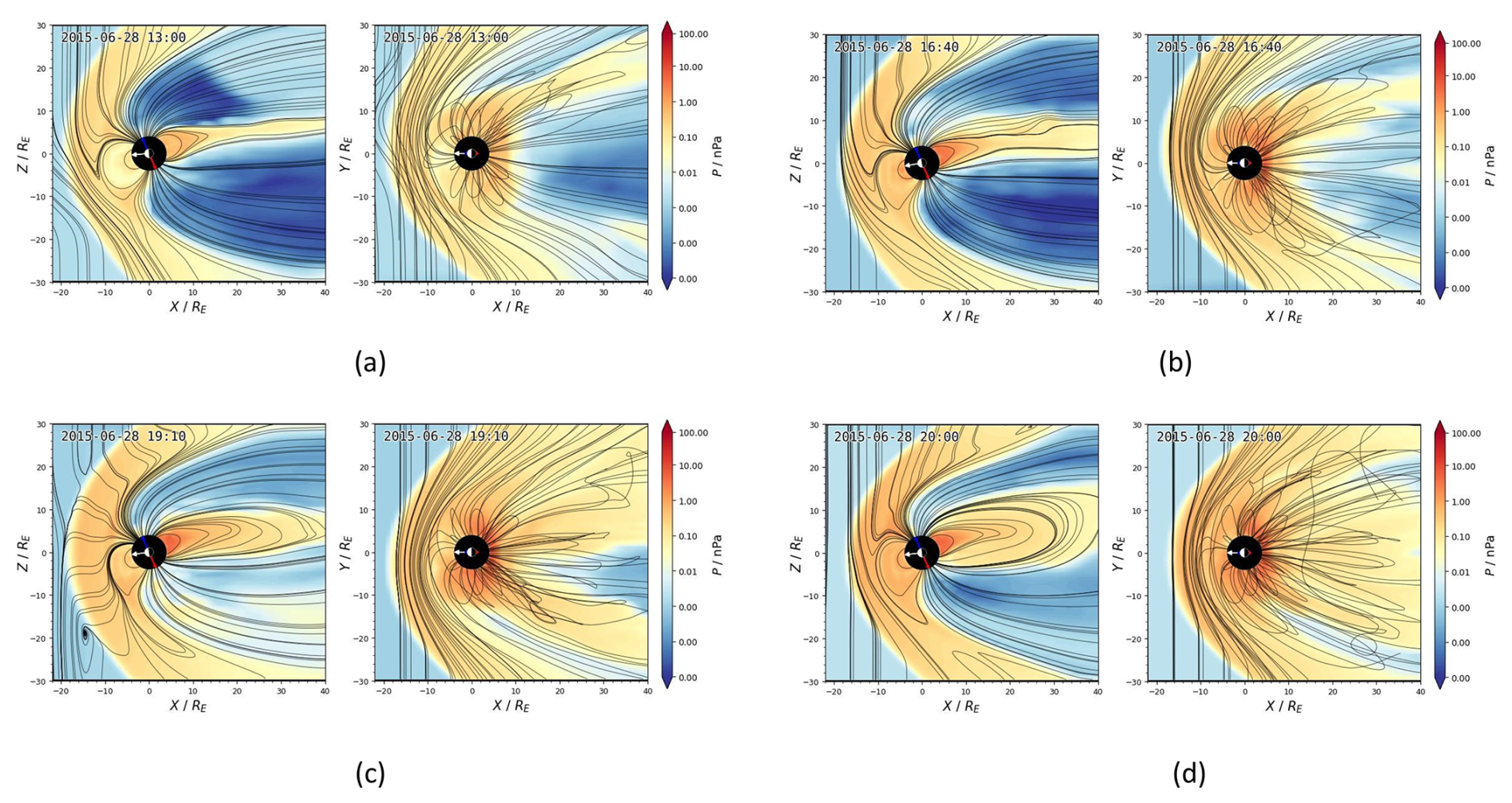
Figure 4 Snapshot of thermal pressure from the MHD simulation with Gorgon-Space. It depicts the arrival time of the second CME, which began on 25 June 2015 at 14:53 and reached Earth on 28 June 2015 at 12:52 UT, in the noon-midnight plane. All panels are shown in GSE coordinates. Note that the x and y axes in GSE are opposite to those in GSM.

Accurate prediction of CME arrival times must account for magnetospheric shielding and internal reconfiguration effects; neglecting them can lead to overestimation of direct solar-wind coupling and mischaracterisation of the geomagnetic response. The dynamic pressure and magnetic topology during the CME2 impact are shown in Fig. 4. A comparison with the pre-CME state in Fig. 3 reveals the extreme compression caused by CME1. The magnetopause and bow shock are pushed inward to approximately $X/R_{\mathrm{E}}\sim \mathrm{10}$ for CME1 (i.e., 10 Earth radii from the centre), whereas they are located around $X/R_{\mathrm{E}}\sim \mathrm{20}$ for the weaker CME2. This dramatic difference in standoff distance reflects the much stronger dynamic pressure of the solar wind during CME1. The magnetosphere continues to deflect most of the solar wind, thereby shielding the inner region, albeit within a significantly reduced and deformed volume.

In other words, the MHD simulations reveal a stark contrast in magnetospheric response between the strong CME1 and the weak CME2. The arrival of CME1 (Fig. 3) induces severe compression of the dayside magnetopause and a significant enhancement of solar wind pressure throughout the magnetosphere, resulting in a highly distorted, elongated tail structure. In contrast, the weaker CME2 (Fig. 4) produces only a moderate compression of the magnetopause and a much less pronounced increase in pressure, resulting in a magnetospheric configuration that remains closer to its nominal state, with a less perturbed tail. This demonstrates a direct correlation between CME intensity and the degree of global magnetospheric deformation and pressure loading.

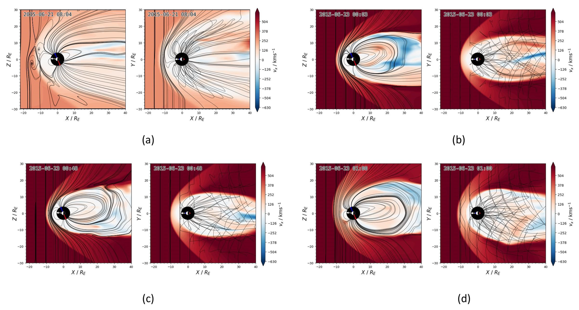
Figure 5 Snapshot of flowvelocity from the MHD simulation with Gorgon-Space. It depicts the arrival time of the first CME, which began on 21 June 2015 at 08:02 and reached Earth on 23 June 2015 at 00:03 UT, in the noon-midnight plane. All panels are shown in GSE coordinates.

Figure 5 depicts the changes in velocity caused by the CME1 at the magnetosphere. The first panel of Fig. 5 shows that the speed at the time of CME1 happening on the Sun is not noteworthy. Additionally, the magnetospheric magnetic field has a consistent shape and can fulfil its primary role as a protective barrier. Panels (b) to (d) depict the wind speed and magnetic configuration of the magnetosphere upon the arrival of CME1 at Earth. Upon initial observation, these three panels represent a notable degree of speed and an irregular magnetic structure resulting from the interaction between the solar wind and the magnetosphere. One can infer that energy from the solar wind is transferred to the Earth's magnetosphere via magnetic reconnection. This occurs when the interplanetary magnetic field connects to the Earth's magnetic field at the magnetopause on the planet's dayside.

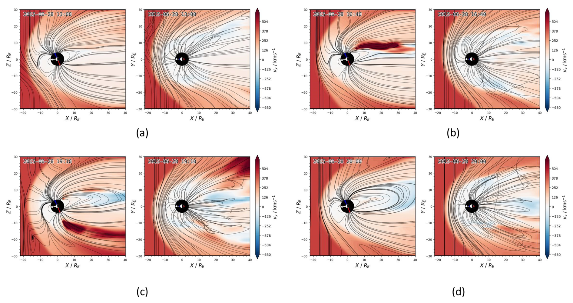
Figure 6 Snapshot of flow velocity from the MHD simulation with Gorgon-Space. It depicts the arrival time of the second CME, which began on 25 June 2015 at 14:52 and reached Earth on 28 June 2015 at 12:52 UT, in the noon-midnight plane. All panels are shown in GSE coordinates.

Figure 6 depicts the flow velocity and magnetic field configuration upon CME2's arrival at Earth. CME2 does not lead to high plasma velocity in the magnetosphere. Besides, in Fig. 6, in the x–z plane, the closed-field regions are larger on the nightside, which could be due to a reduction in open-flux content in the magnetosphere. This might lead to decreased geomagnetic activity and smaller polar caps in the ionosphere.

The rate of magnetic reconnection and the amount of energy transferred are influenced by the solar wind speed, magnetic field strength, and orientation. Subsequently, it was discovered that CME1 triggers a significant tempest on Earth and is accompanied by changes in the magnetic arrangement, increased speed and pressure of the solar wind enveloping the Earth, as previously anticipated in Fig. 2.

Figure 4 showcases the changes in pressure and magnetic field in the vicinity of the Earth upon the arrival of CME2. As shown in Fig. 2, there was no indication of a significant magnetic storm when CME2 arrived. It can shed light on the impact of the background solar wind, which is the same in both CMEs, and thus it is not the primary factor in causing magnetic storms. Hence, it can be deduced that the nature of the CME and its interactions with other CMEs are crucial factors in determining the geomagnetic impact of CMEs on Earth.

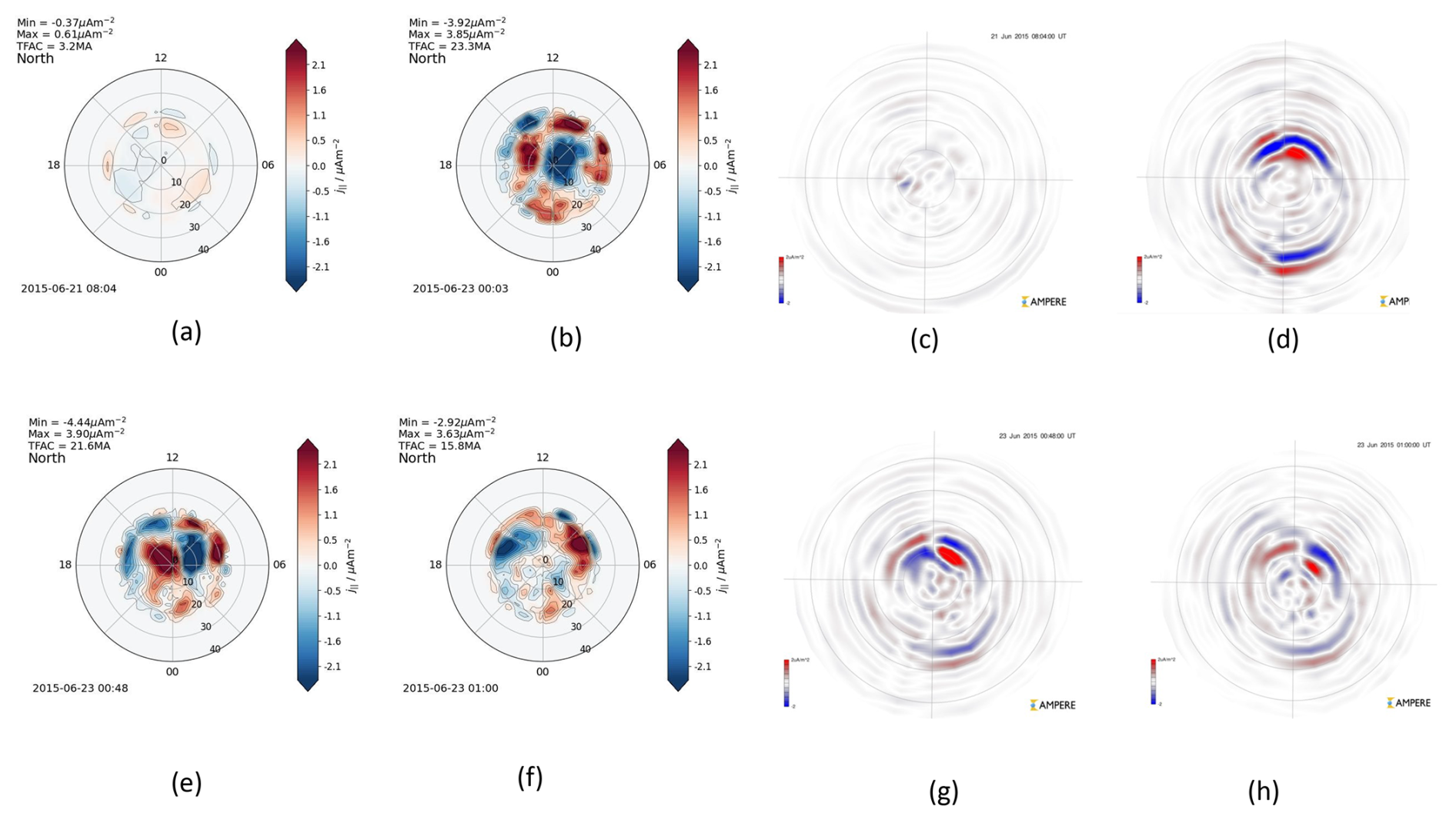
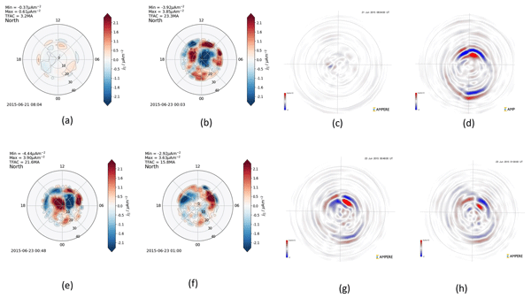
Figure 7 Comparison of field-aligned currents (FACs) from Gorgon-Space (left columns) and AMPERE observations (right columns) for the CME1 event. Red indicates upward currents (out of the ionosphere); blue indicates downward currents (into the ionosphere). Panels (a) and (c) show the quiet-time pre-impact baseline (21 June, 08:04 UT), where both datasets exhibit weak, patchy currents. Panels (b) and (d) show the sudden commencement at 00:03 UT on 23 June, revealing the rapid intensification of the Region-1/Region-2 FAC system. Panels (e) and (g) capture the main phase peak at 00:48 UT, when the classic two-cell convection pattern is well established. Panels (f) and (h) show the post-MI decay phase at 01:00 UT, with the current system beginning to decay. The close agreement in morphology and timing validates the model's magnetosphere-ionosphere coupling and the dynamic conductance model.

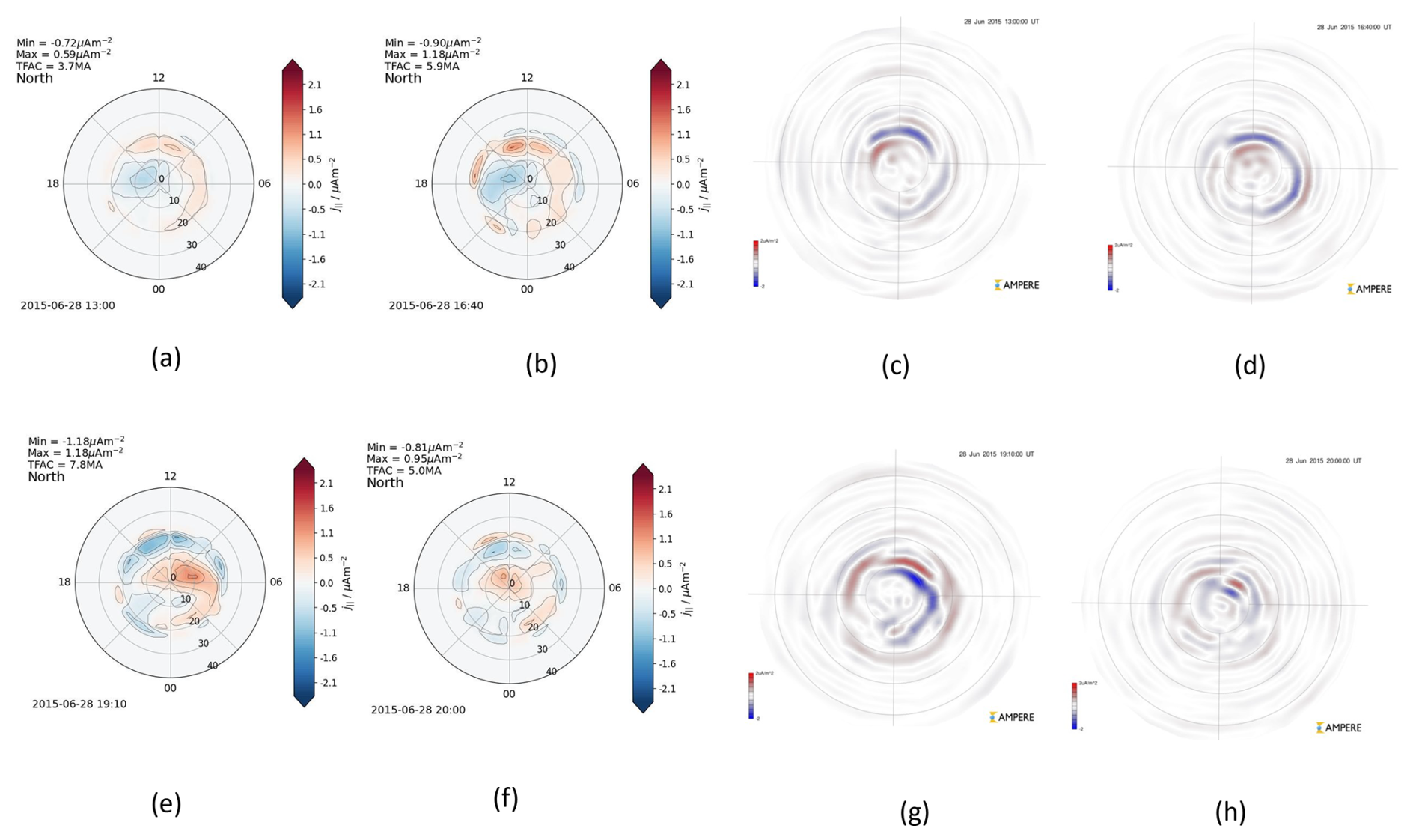
Figure 8 Comparison of field-aligned currents (FACs) from Gorgon-Space (left column) and AMPERE observations (right column) for the CME2 event (28 June 2015). (a) Model at 13:00 UT; (b) Model at 16:40 UT; (c) AMPERE at 13:00 UT; (d) AMPERE at 16:40 UT; (e) Model at 19:10 UT; (f) AMPERE at 20:00 UT. Red indicates upward currents (out of the ionosphere); blue indicates downward currents (into the ionosphere). In contrast to CME1 (Fig. 7), both model and AMPERE show weak and disorganised FACs with total integrated currents below 8 MA, reflecting the minimal geoeffectiveness of CME2 due to the absence of sustained southward IMF.

This enhanced energy input for CME1 directly explains the observed magnetospheric compression, tail stretching, and nightside plasmoid formation (Fig. 3), as well as the intense field-aligned currents exceeding 23 MA (Fig. 7) and the elevated cross-polar cap potential of ∼160 kV (Fig. 9). For CME2, the minimal reconnection activity results in negligible energy transfer, consistent with the absence of significant magnetospheric distortion (Fig. 4), weak FACs (Fig. 8), and low ionospheric convection potential (Fig. 10).

3.2 Ionospheric Response

To model magnetosphere–ionosphere (M–I) coupling, Gorgon-Space employs a separate, height-integrated ionospheric module. The 3D MHD domain does not resolve the ionosphere; instead, its inner boundary is placed at R_IB=4 R_E, where field-aligned currents (FACs) are computed from the magnetospheric solution via Ampère's law, ${\mathbf{J}}_{\parallel }=(\mathbf{J}\cdot \mathit{b})\mathit{b}$, with $\mathit{b}=\mathit{B}/\left|\mathit{B}\right|$. These FACs are mapped along dipole magnetic field lines onto a 2D spherical ionospheric grid at an effective altitude of ∼110 km – corresponding to the E region (90–150 km), where Hall and Pedersen conductivities peak.

In the Gorgon-Space model, the ionospheric electrical conductivity is represented by height-integrated Pedersen (Σ_P) and Hall (Σ_H) conductances. These are calculated using a combination of solar EUV-driven background and auroral precipitation-driven enhancements:

$$\begin{array}{}\text{(6)}& {\displaystyle }{\mathrm{\Sigma }}_{\mathrm{P}}={\mathrm{\Sigma }}_{\mathrm{P},\mathrm{EUV}}+{\mathrm{\Sigma }}_{\mathrm{P},\mathrm{aurora}}\text{(7)}& {\displaystyle }{\mathrm{\Sigma }}_{\mathrm{H}}={\mathrm{\Sigma }}_{\mathrm{H},\mathrm{EUV}}+{\mathrm{\Sigma }}_{\mathrm{H},\mathrm{aurora}}\end{array}$$

EUV-driven background. The solar EUV contribution is parameterized as a function of solar zenith angle (χ) and the F10.7 solar flux index (in sfu, $\mathrm{1}\mathrm{sfu}={\mathrm{10}}^{-\mathrm{22}}\mathrm{W}{\mathrm{m}}^{-\mathrm{2}}{\mathrm{Hz}}^{-\mathrm{1}}$):

$$\begin{array}{}\text{(8)}& {\displaystyle }{\mathrm{\Sigma }}_{\mathrm{P},\mathrm{EUV}}=\mathrm{5.0}\times {\left({\displaystyle \frac{\text{F10.7}}{\mathrm{100}}}\right)}^{\mathrm{0.5}}\times \cos (\mathit{\chi }{)}^{\mathrm{0.5}}\text{(9)}& {\displaystyle }{\mathrm{\Sigma }}_{\mathrm{H},\mathrm{EUV}}=\mathrm{0.8}\times {\mathrm{\Sigma }}_{\mathrm{P},\mathrm{EUV}}\end{array}$$

These empirical relations follow the standard formulation used in many global MHD models (e.g., Ridley et al., 2004; Wiltberger et al., 2017), where the cos ^0.5(χ) dependence approximates the Chapman production function for ionospheric ionization.

Auroral component. The auroral contribution is derived from the mapped magnetospheric electron energy flux (ε, in mW m⁻²) and characteristic energy (E₀, in keV) using the empirical relations of Robinson et al. (1987):

$$\begin{array}{}\text{(10)}& {\displaystyle }{\mathrm{\Sigma }}_{\mathrm{P},\mathrm{aurora}}={\displaystyle \frac{\mathrm{40}\mathit{\epsilon }{E}_{\mathrm{0}}}{\mathrm{16}+E_{\mathrm{0}}^{\mathrm{2}}}}\text{(11)}& {\displaystyle }{\mathrm{\Sigma }}_{\mathrm{H},\mathrm{aurora}}={\displaystyle \frac{\mathrm{40}\mathit{\epsilon }{E}_{\mathrm{0}}^{\mathrm{0.85}}}{\mathrm{16}+E_{\mathrm{0}}^{\mathrm{2}}}}\end{array}$$

These relations are derived from fits to auroral observations and have been widely validated for storm-time conditions (Robinson et al., 1987; Ridley et al., 2004). The factor 40 has units of $\mathrm{m}{\mathrm{W}}^{-\mathrm{1}}{\mathrm{m}}^{\mathrm{2}}{\mathrm{keV}}^{-\mathrm{1}}$ to produce conductances in siemens.

During the simulation, the electron energy flux and characteristic energy at the inner boundary (R=4 R_E) are mapped along dipole field lines to the ionospheric altitude (∼110 km). The conductances are updated at each time step (Δt≈10 s) to reflect changes in magnetospheric precipitation.

The total ionospheric conductance (Σ_P, Σ_H) is then used in Ohm's law for the height-integrated ionospheric current:

$$\begin{array}{}\text{(12)}& {\mathbf{J}}_{⟂}={\mathrm{\Sigma }}_{\mathrm{P}}\mathit{E}+{\mathrm{\Sigma }}_{\mathrm{H}}(\mathit{B}\times \mathit{E})\end{array}$$

where E is the ionospheric electric field, b is the unit vector of the magnetic field, and J_⟂ is the height-integrated perpendicular current density. This dynamic conductance model is critical for accurately reproducing the observed FAC intensities and cross-polar cap potentials during the storm main phase. The Gorgon-Space code has been previously validated for ionospheric coupling and FAC simulations under storm-time conditions (Eggington et al., 2020; Mejnertsen et al., 2018). In a recent study using the same EUHFORIA-Gorgon-Space modelling chain to investigate the May 2024 solar storm, Sabri et al. (2025) further demonstrated that the dynamic conductance model successfully reproduced observed FAC patterns and cross-polar-cap potentials measured by SuperDARN, providing additional validation of this implementation.

The electrostatic potential ϕ is obtained by solving the 2D current continuity equation:

$$\begin{array}{}\text{(13)}& {\mathrm{\nabla }}_{⟂}\cdot {\mathbf{J}}_{⟂}=-{\mathrm{\nabla }}_{⟂}\cdot \left({\mathrm{\Sigma }}_{\mathrm{P}}{\mathrm{\nabla }}_{⟂}\mathit{\varphi }\right)=J_{\parallel }\end{array}$$

ensuring current closure. The resulting potential distribution is mapped back along the dipole field lines to the MHD inner boundary, thereby providing a self-consistent time-dependent boundary condition for the plasma flow.

Within the thin-shell approximation, the height-integrated ionospheric current is governed by Ohm's law: ${\mathbf{J}}_{⟂}={\mathrm{\Sigma }}_{\mathrm{P}}\mathit{E}+{\mathrm{\Sigma }}_{\mathrm{H}}(\mathit{b}\times \mathit{E})$, where Σ_P and Σ_H are the Pedersen and Hall conductances. In this study, these conductances are calculated using empirical relations: a solar EUV-driven background (with square-root dependence on solar flux) and an auroral component derived from magnetospheric electron energy flux mapped along field lines. The electrostatic potential ϕ is obtained by solving the 2D current continuity equation ${\mathrm{\nabla }}_{⟂}\cdot {\mathbf{J}}_{⟂}=-{\mathrm{\nabla }}_{⟂}\cdot \left({\mathrm{\Sigma }}_P{\mathrm{\nabla }}_{⟂}\mathit{\varphi }\right)=J_{\parallel }$, ensuring current closure. The resulting potential distribution is mapped back along the dipole field lines to the MHD inner boundary, thereby providing a self-consistent time-dependent boundary condition for the plasma flow.

This coupling enables energy and momentum transfer across the system: FACs generated in the magnetosphere (where $\mathrm{\nabla }\times \mathit{B}\ne \mathrm{0}$) flow into the ionosphere, where they are closed by perpendicular Pedersen and Hall currents. The resulting Lorentz force, ${\mathbf{J}}_{⟂}\times \mathit{B}$, drives ionospheric plasma convection and, through ion–neutral collisions, neutral winds. This convection pattern, anchored by FAC stress, transports magnetic flux tubes globally, thereby mediating the large-scale M–I energy exchange that underpins space-weather impacts.

The accumulation of current density aligned with the magnetic field can be attributed to the interaction between the solar wind and the magnetosphere. The predominant energy transfer and current alignment in the ionosphere were driven primarily by the boundary conditions. To accurately predict space weather, it is necessary to have a solid understanding of the physics underlying these coupling processes. Determining the accuracy of MHD codes in reproducing plasma sheet electric fields during solar wind-magnetosphere interactions is of utmost significance for Space Weather applications.

Figure 7 presents the evolution of field-aligned current (FAC) density in the Northern Hemisphere ionosphere in response to the sudden commencement (SC) driven by the arrival of CME1 at Earth, capturing the onset, peak, and initial recovery of the disturbance. Panel (a) shows the quiet-time pre-impact baseline at 08:02 UT on 21 June. Following the SC, panels (b) and (c) depict the development and peak of the intense electrodynamic response. Panel (b), immediately after the SC at 00:03 UT on 23 June, reveals a localized, dayside-enhanced FAC pattern. This initial enhancement is consistent with the characteristic Preliminary Impulse (PI) observed during shock-induced compressions, often attributed to the compression of the dayside magnetosphere and the associated Chapman-Ferraro (CF) currents (e.g., Araki, 1994).

Panel (c) shows the peak intensity, indicating a substantial increase in the total current magnitude to approximately 23 MA and a poleward shift of the primary current regions. This stronger, poleward-expanding structure corresponds to the Main Impulse (MI). The MI signifies the full engagement of the global current system (R1 FACs), which is directly driven by the large-scale magnetospheric convection electric field. This convection electric field (${\mathit{E}}_{\mathrm{conv}}=-v\times \mathit{B}$) is itself established by enhanced dayside magnetic reconnection under the prolonged southward IMF conditions in the CME sheath.

Panel (d) shows the onset of the post-MI decay phase in the Northern Hemisphere, where the current density magnitude decreases, and the pattern shifts poleward from 0 to 10–20° colatitude. The clear temporal sequence from quiet conditions (a) through the distinct PI and MI phases (b, c) and into post-MI decay (d) demonstrates that the Gorgon-Space code captures the fundamental two-phase ionospheric electrodynamic response to a CME-driven shock, a key benchmark for validating space-weather models. The intense MI-phase FACs are a primary conduit for energy transfer from the magnetosphere, underscoring their critical role in driving space-weather effects such as geomagnetically induced currents (Pulkkinen, 2007; Pirjola, 2005).

To validate the magnetosphere-ionosphere coupling in our simulations, we compare the Gorgon-Space-derived field-aligned current (FAC) distributions with observational data from the Active Magnetosphere and Planetary Electrodynamics Response Experiment (AMPERE). Figure 7 presents a side-by-side comparison of modelled (left) and AMPERE-observed (right) FAC densities in the Northern Hemisphere at four key stages of the CME1 event.

Panel (a) shows the quiet-time pre-impact baseline (21 June, 08:04 UT), where both datasets exhibit weak, patchy currents with total integrated FAC <5 MA. Following the sudden commencement at 00:03 UT (panel b), both the model and AMPERE show a rapid intensification of the Region 1/Region 2 FAC system, with peak densities exceeding ±1 µA m⁻² and total integrated currents reaching approximately 23 MA in the simulation.

During the main-phase peak at 00:48 UT (panel c), the classic two-cell convection pattern is well established in both datasets, with strong dawnside downward (blue) and duskside upward (red) currents. By 01:00 UT (panel d), the system begins to decay, though residual currents remain elevated at approximately 15–18 MA in the model.

The close agreement in morphology, timing, and integrated current magnitude validates the dynamic conductance model and the EUHFORIA-derived upstream boundary conditions. Minor discrepancies in fine-scale structures are expected: AMPERE's ∼10–20 min temporal resolution and spatial smoothing differ from the model's grid-scale output, and current wedges are not fully resolved in the global MHD framework. Nevertheless, the large-scale FAC evolution is robustly captured, confirming the model's fidelity for space weather applications.

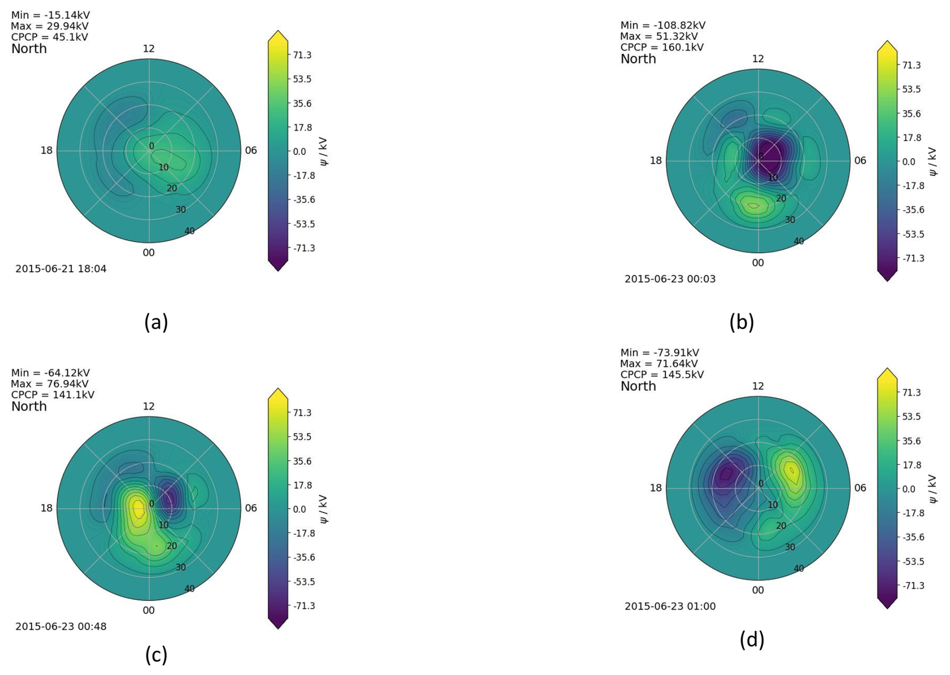
Figure 9 Ionospheric response electric potential during the happening of the first CME and its arriving at the Earth. Yellow indicates the positive potential, and blue means negative potential.

For completeness, we also compare the Gorgon-Space-simulated FACs with AMPERE observations for the CME2 event (28 June 2015). Figure 8 presents this comparison at three key times during the CME2 passage.

Panel (a) shows the model prediction at 13:00 UT, shortly after the CME2 arrival. The FACs are weak and disorganized, with a total integrated current of only 3.7 MA and peak densities ranging from −0.72 to +0.59 µA m⁻². The corresponding AMPERE observations (panel c) confirm this weak activity, showing no clear Region-1/Region-2 structure.

At 16:40 UT (panels b and d), both the model and AMPERE show a slight intensification, with total FAC reaching 7.8 MA in the model and 5.0 MA in AMPERE. However, the currents remain significantly weaker than those observed during CME1 (in which the total FAC exceeded 23 MA). The pattern remains disorganized, lacking the classic two-cell convection structure.

By 19:10–20:00 UT (panels e and f), the FACs begin to decay further. The model predicts a total FAC of 7.5 MA, while AMPERE shows 5.0 MA. The close agreement between model and observations in capturing the weak, disorganized nature of the FACs during CME2 validates the model's ability to correctly simulate both geoeffective (CME1) and non-geoeffective (CME2) events. This demonstrates that the EUHFORIA-Gorgon-Space chain correctly reproduces the observed contrast between the two CMEs as a function of IMF orientation.

Minor discrepancies in the exact timing of peak currents are expected due to AMPERE's ∼10–20 min temporal resolution and the inherent variability in CME-solar wind interactions. Nevertheless, the overall agreement confirms that the model successfully captures the muted ionospheric response to CME2, consistent with the absence of sustained southward IMF.

Table 2 Comparison of field-aligned currents (FACs) and geoeffectiveness between CME1 and CME2.

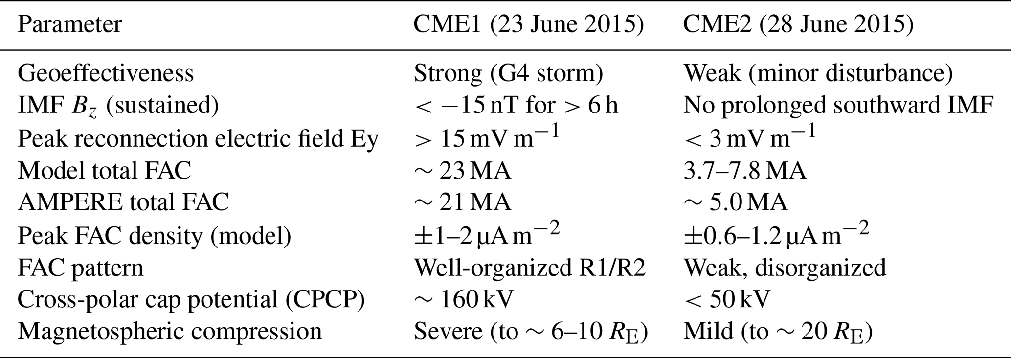
Table 2 summarizes the key differences between the two CME events. CME1 produced a strong geomagnetic storm (G4 level) with intense FACs (∼23 MA), high CPCP (∼160 kV), and severe magnetospheric compression. In contrast, CME2 produced only weak FACs (<8 MA) and minimal geoeffectiveness, despite having a higher peak speed. This contrast confirms that IMF orientation, not CME speed, governs storm intensity.

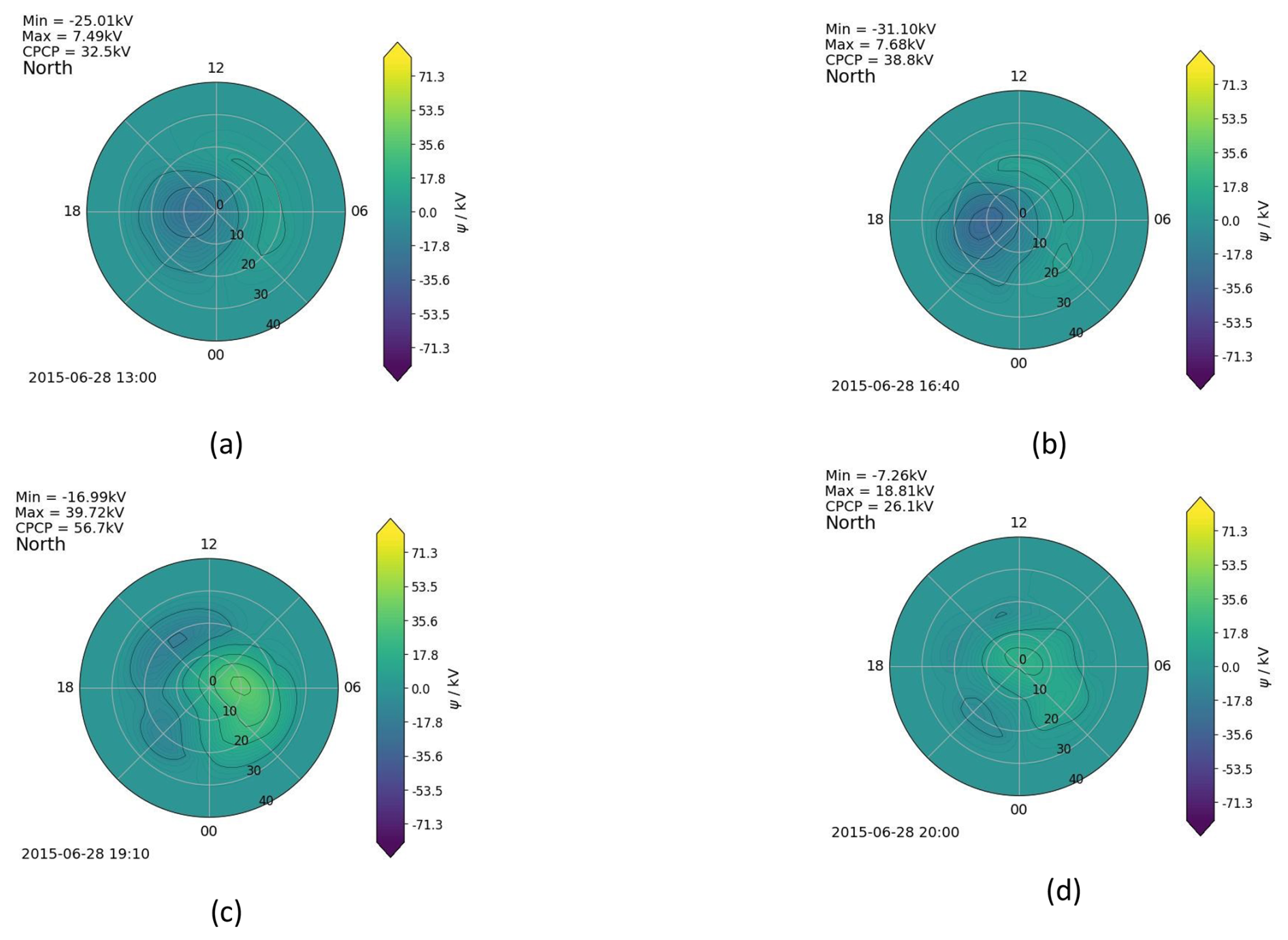
Figure 10 Ionospheric response electric potential during the arrival of CME2 at Earth. Yellow indicates the positive potential, and blue means negative potential.

Figure 9 shows the electric potential response in the ionosphere. The illustration shows the cross-polar cap electric potential (CPCP) in the ionosphere, which is widely used to assess the worldwide convection intensity. This shows the disparities between the highest and lowest electric potential values in the ionosphere. CPCP was initially derived from the integral rate of dayside-merging and can be used as an estimate of the key parameter of dayside-merging, as in Gordeev et al. (2015).

The first panel in Fig. 9 shows the level of the electric potential in the ionosphere at the onset of the initial coronal mass ejection (CME1). Panel (b) of Fig. 9 displays the ionospheric electric potential reaction during the initial arrival of the first coronal mass ejection (CME1) at the Earth. Comparing the two panels helps determine the impact of the solar wind on Earth, yielding an ionospheric electric potential of approximately 160 kV during the CME1 impact. This elevated cross-polar cap potential (∼160 kV) is a direct measure of the strength of the magnetospheric convection electric field. This same convection electric field, when mapped back along magnetic field lines into the magnetosphere, drives the bulk plasma motion via the E×B drift. Consequently, the weak ionospheric potential during CME2 (Fig. 10) is physically consistent with the low plasma velocities observed in the magnetosphere for that event (Figs. 5, 6). Figure 10 illustrates the electric potential in the ionosphere when CME2 reaches the Earth. As predicted, the arrival of CME2 at Earth does not cause any notable electric potential in the ionosphere. The elevated ionospheric potential (∼160 kV) is a signature of a strong magnetospheric convection electric field. This large-scale field governs the global transport and energisation of plasma. While the quasi-static ionospheric field itself does not directly accelerate particles to high energies, the associated magnetospheric convection can inject plasma-sheet particles into the inner magnetosphere, where they may subsequently be accelerated to ring-current and radiation-belt energies by processes such as radial diffusion and wave-particle interactions.

4 Conclusions

Because of their profound impacts on both scientific understanding and technological systems, coronal mass ejections (CMEs) remain a central focus of space weather research. CMEs drive intense geomagnetic storms, capable of enhancing radiation belt fluxes that threaten satellites, and can produce solar energetic particles (SEPs) that disrupt spacecraft operations and aviation safety. Understanding how CME properties, such as speed, magnetic structure, and interaction with the ambient solar wind or other CMEs, determine their geoeffectiveness is therefore critical.

In this study, we examined two CMEs that impacted Earth on 23 and 28 June 2015 (identified as CME1 and CME2 in Sabri and Poedts, 2025), which exhibited markedly different geoeffectiveness despite both being fast events. Using an end-to-end modelling chain that couples the EUHFORIA heliospheric model to the Gorgon-Space global MHD code, we performed time-dependent, 3D simulations of the resulting magnetospheric and ionospheric responses.

Our key findings are as follows:

1. CME1 induced firm compression of the dayside magnetosphere and pronounced tailward stretching in the xy plane, consistent with enhanced magnetic reconnection under sustained southward IMF conditions. This led to significant deformation of the bow shock and magnetopause boundaries.

2. CME1 triggered a major geomagnetic storm, characterised by a total field-aligned current (FAC) of approximately 23 MA concentrated in the Northern Hemisphere ionosphere, reflecting intense energy deposition from the magnetosphere.

3. In contrast to CME1, CME2 produced only weak FACs (total integrated current <8 MA) with a disorganized spatial pattern, as confirmed by both Gorgon-Space simulations and AMPERE observations. This demonstrates that the model correctly captures the muted ionospheric response to CME2, consistent with the absence of sustained southward IMF.

4. The ionospheric cross-polar cap potential (CPCP) reached ∼160 kV during CME1, consistent with strong convection driven by dayside reconnection. This electric potential facilitates the transport of plasma-sheet particles toward Earth, thereby supporting ring-current growth and auroral precipitation.

5. The close temporal correspondence between EUHFORIA's predicted solar wind conditions at L1 and the magnetospheric–ionospheric response simulated by Gorgon-Space – evident in the accurately reproduced timing of magnetopause compression, field-aligned current intensification, and cross-polar cap potential evolution – demonstrates that our coupled modeling system captures the expected causal chain of solar wind–magnetosphere coupling. This agreement validates the self-consistency and predictive capability of the EUHFORIA–Gorgon-Space framework.

This work makes three distinct contributions to space weather forecasting:

1. Operational validation. We demonstrate the first end-to-end EUHFORIA→Gorgon-Space chain that accurately forecasts magnetospheric drivers (FACs >23 MA, CPCP 160 kV) from heliospheric CME parameters, a critical capability for predicting geomagnetically induced current (GIC) risks to power grids.

2. Physics-based discrimination. By resolving the CME1/CME2 contrast, we provide a quantitative, model-based demonstration that IMF orientation (not speed) controls storm intensity – enabling forecasters to reject false alarms from fast CMEs with unfavourable magnetic geometry.

3. Numerical robustness. Gorgon-Space's $\mathrm{\nabla }\cdot \mathit{B}=\mathrm{0}$-preserving formulation captures extreme magnetospheric compression during CME impacts without numerical instabilities – a prerequisite for reliable operational forecasting during extreme events.

Unlike previous end-to-end modeling studies that stop at magnetospheric boundaries, our EUHFORIA-Gorgon-Space chain quantifies the complete energy pathway from heliospheric CME parameters to ionospheric electrodynamic impacts (FACs, convection potentials). This bridges a critical gap in operational space-weather forecasting by translating L1 solar wind measurements into actionable GIC risk assessments for power grid operators.

This work demonstrates that Gorgon-Space, with its divergence-free magnetic-field formulation and validated ionosphere coupling, provides a robust platform for translating heliospheric CME forecasts into quantifiable space-weather impacts in near-Earth space. While global MHD models such as SWMF and OpenGGCM have successfully simulated storm-time magnetospheres, few studies have examined the transient, high-fidelity evolution of field-aligned currents during the initial compression and main phase of CME-driven storms using a $\mathrm{\nabla }\cdot \mathit{B}=\mathrm{0}$-preserving code. Gorgon-Space's vector-potential formulation provides numerical stability during extreme compressions, enabling accurate capture of FAC dynamics that drive geomagnetically induced currents (GICs). This study demonstrates the first application of the EUHFORIA–Gorgon-Space chain to resolve the complete sequence from CME launch to the ionospheric electrodynamic response, offering a validated framework for operational space-weather forecasting. Future work will include a quantitative comparison with SuperMAG-derived auroral electrojet (AE/AL/AU) indices to further validate the evolution of the ionospheric current system.