High-latitude observations of ULF wave driven ion upflow

We present a comprehensive study of the first observations of ionospheric ion upflow generated by ultra-low frequency (ULF) wave driven auroral arcs (UAAs). Ground- and space-based instrumentation, together with inversion models, allow us to study the event at different length scales. This shows the complex dynamics of UAAs and their role in the ionosphere-magnetosphere coupling via ion upflow, field-aligned currents (FACs), and energy dissipation. The UAA event was observed as a series of six poleward moving arcs, primarily in the 630.0 nm emission line. At the northern extent of the arcs incoherent scatter radar (ISR) data indicated that the UAAs have driven type 2 ion upflow with low to medium fluxes of around 3.3×10¹³ particles m⁻² s⁻¹. Data from the ISR, spacecraft, and models, result in FAC magnitudes up to 6 µA m⁻², total energy fluxes up to 12 mW m⁻², and Joule heating rates up to 11 mW m⁻² associated with the arcs. These values mostly correspond to localized measurements, while at large-scale the values are up to 50 % smaller. In addition, ground-based magnetometers suggested that the UAA event is driven by small-scale ULF waves, while energy dissipation rates and FAC magnitudes are significant and comparable to previously reported large-scale wave events, indicating the importance of using a multi-instrument approach when investigating energy dissipation associated with ULF waves. This event thus shows that even small-scale ULF waves can drive ion upflow in the ionosphere.

1 Introduction

Ion outflow plays a fundamental role in the ionosphere – magnetosphere coupling and outflows contribute significantly to the magnetospheric plasma population (Bjoland et al., 2025). At high-latitudes, ions of ionospheric origin can be energized and lifted to higher altitudes (upflow) where they may escape into the magnetosphere and interplanetary region (outflow). Originally, ion upflow has been categorized into two types where the first is driven by ion heating (type 1) and the second by electron heating (type 2) (Wahlund et al., 1992). Type 1 upflow is characterized by strong perpendicular electric fields, enhanced ion temperatures down to the E region, and low electron densities below 300 km, suggesting a lack of auroral precipitation. The enhanced ion temperature can cause a pressure gradient that accelerates ions upward. Type 2 upflow is associated with enhanced electron temperatures and densities, and is related to auroral arcs. The enhanced electron temperature can lead to an increase in the ambipolar electric field, which then causes ion upflow. Later studies confirmed that these mechanisms often act simultaneously, showing both enhanced electron and ion temperatures and producing complex ionospheric signatures (Skjæveland et al., 2011).

The European Incoherent Scatter (EISCAT) Svalbard radar (ESR) has been a key instrument in quantifying ion upflow fluxes and statistical characterization of ion upflow (e.g. Ogawa et al., 2009; Ji et al., 2019; Ogawa et al., 2003; Skjæveland et al., 2011, 2014; David et al., 2018, 2024; Bjoland et al., 2025). Most upflow studies focus on the dayside ionosphere, but upflow can happen during all magnetic local times. To separate genuine upflow and downflow from noise in the ESR data, Ogawa et al. (2009) used a threshold of +100 m s⁻¹ (−100 m s⁻¹) at three or more consecutive heights along the profile to detect ion upflow (downflow). Subsequent long-term ESR data sets reveal that ion upflow fluxes above Svalbard typically average at 10¹³ particles m⁻² s⁻¹, but exhibit strong variability with magnetic local time, season, and geomagnetic activity (Ogawa et al., 2011; David et al., 2018). It is possible to divide ion upflow fluxes, f_i, into three categories: low ($\mathrm{1.0}\times {\mathrm{10}}^{\mathrm{13}}\le f_{\mathrm{i}}\le \mathrm{2.5}\times {\mathrm{10}}^{\mathrm{13}}$ m⁻² s⁻¹), medium ($\mathrm{2.5}\times {\mathrm{10}}^{\mathrm{13}}\le f_{\mathrm{i}}\le \mathrm{7.5}\times {\mathrm{10}}^{\mathrm{13}}$ m⁻² s⁻¹), and high ($f_{\mathrm{i}}\ge \mathrm{7.5}\times {\mathrm{10}}^{\mathrm{13}}$ m⁻² s⁻¹) (David et al., 2018). Low flux upflows occur most often, while medium and high fluxes are largely linked to enhanced geomagnetic conditions.

Ion upflow has been associated with auroral optical emissions in general (Zettergren et al., 2007), and more specifically poleward moving auroral forms (PMAFs) (Skjæveland et al., 2011), pulsating aurora (Godbole et al., 2022), continuum emission (Partamies et al., 2025), and auroral arcs (Lynch et al., 2007), among others.

Another important factor in the redistribution and transport of energy within the Earth's magnetosphere are ultra-low frequency (ULF) waves. ULF waves are oscillations ranging from 1 mHz to 1 Hz that can often be described with a magnetohydrodynamic (MHD) approximation, and can be observed as Alfvén and compressional waves. One of the most commonly observed types of ULF waves in the Earth's ionosphere is the field line resonance (FLR), a large-scale, standing Alfvén wave that occurs on closed magnetic field lines and transports energy and momentum along these field lines. The azimuthal scale size of ULF waves is described by the m-number ($m=\mathrm{2}\mathit{\pi }{R}_{\mathrm{E}}\cos \mathit{\theta }/{\mathit{\lambda }}_{\mathrm{az}}$, where R_E is the Earth's radius, θ the geographic latitude, and λ_az the azimuthal wavelength in the ionosphere). Waves can be classified according to their m-number, where low-m waves have large spatial scales and are predominantly toroidally polarized. Although there are no strict definitions regarding scale sizes, low-m waves typically have m numbers between 1–10 and include FLRs, which are most effectively driven by fast mode waves when m≈3 (Menk and Waters, 2013; Rubtsov et al., 2018). High-m waves, on the other hand, have small spatial scales and show poloidal polarization. Waves are generally considered high-m when m>15 (Yeoman et al., 2010), but in other cases even higher values such as $\mathrm{50}<m<\mathrm{150}$ are used for the high-m classification (Mager et al., 2019; Michael et al., 2024). In between low-m and high-m was, there is a class of intermediate-m waves ($\mathrm{10}\lesssim m\lesssim \mathrm{15}$) which can show characteristics of either low-m or high-m waves (Mager et al., 2019). Above Svalbard, at θ=77°, large-scale waves (m<10) correspond to azimuthal length scales of λ_az>900 km, while small-scale waves (m>15) are characterized by λ_az<600 km. Optically, ULF waves can be observed by a periodic series of poleward or equatorward moving auroral arcs, corresponding to ULF wave driven auroral arcs (UAAs) (Gillies et al., 2017, 2018; Van Hazendonk et al., 2025). Traditionally, UAA signatures are associated with FLRs as proposed by the model of Samson et al. (2003), in which the parallel electric fields associated with FLRs can accelerate electrons downward creating these periodic auroral arcs signatures. Recently, Van Hazendonk et al. (2024) indicated that smaller-scale ULF waves could also be associated with UAA signatures in both the dawn and dusk sectors. In addition, Fenrich et al. (2019) associated FLRs with field-aligned currents (FACs) and resolved the two-dimensional (2D) velocities and FACs associated with FLRs, finding typical peak FAC magnitudes around 2–4 µA m⁻², which occurred in localized latitudinal bands with widths of 1–2°. The energy transport of ULF waves consists of electromagnetic energy, as described by the Poynting vector, and kinetic energy (Hartinger et al., 2015; Van Hazendonk et al., 2024). Most studies on the energy budget of ULF waves solely focus on the energy fluxes into the ionosphere, and ignore any potential mass and/or energy flow out of the ionosphere.

In this comprehensive case study of the high-latitude ionosphere, we aim to determine whether UAA events can be associated with energy dissipation, ion upflow and/or outflow. We present a case study taking place on 16 November 2021 above Svalbard. This event was originally detected in the Meridian Scanning Photometer (MSP) statistical study by Van Hazendonk et al. (2025). Ground-based instrumentation, including the ESR, combined with satellite data and models are used to show the complicated nature of this UAA event and its implications on the role that ULF waves play both in terms of energy dissipation into the ionosphere and the flow of mass out of or upwards in the ionosphere.

2 Data

In this study, we used instruments and models with different scale sizes to put together an extensive overview of a UAA event above Svalbard. The ground-based instrumentation includes the EISCAT Svalbard radar (ESR), a meridian scanning photometer (MSP), and ground-based magnetometers. In addition to ground-based data, we used the Defense Meteorological Satellite Program (DMSP), Iridium, and Swarm spacecraft. Solar wind conditions are obtained from ACE and WIND data, shifted to the bow shock nose with 1 min temporal resolution. The DMSP spacecraft carry payloads to measure precipitating auroral particles (Special Sensor for Precipitating Electron and Ion Spectrometer; SSJ (Redmon et al., 2017)), plasma properties including ion drift velocities (Sensor for Ion and Electron Scintillation; SSIES), and optical emissions in ultraviolet and energy fluxes (Special Sensor Ultraviolet Spectrographic Images; SSUSI; (Paxton et al., 1992)), among others. Both the locations of the ground-based instruments as well as the DMSP overpasses are shown in Fig. 1. The ground-based magnetometers in Fig. 1 are from the International Monitor for Auroral Geomagnetic Effects (IMAGE) magnetometer network (Tanskanen, 2009) and are located in Tromsø (TRO), Sorøya (SOR), Bjørnøya (BJN), Hopen (HOP), Hornsund (HOR), Longyearbyen (LYR), and Ny-Ålesund (NAL). Part of the data are used in two models, the ELectron Spectrum (ELSPEC) method (Virtanen et al., 2018) and the Local Mapping of Polar Ionospheric Electrodynamics (Lompe) model (Laundal et al., 2022; Hovland et al., 2022), to determine FACs and energy fluxes.

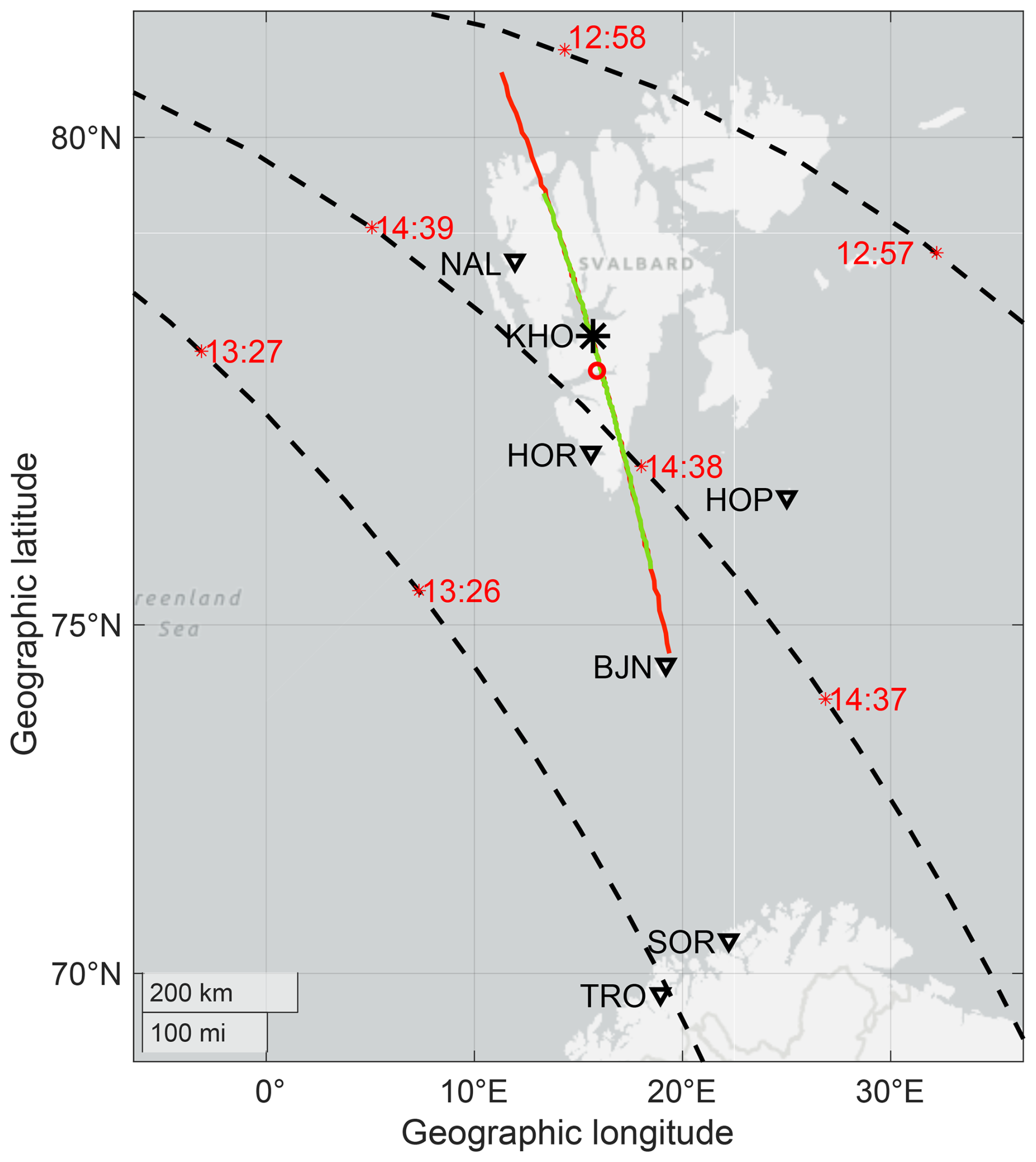
Figure 1 The location of KHO (black star), which coincides with the LYR ground-based magnetometer, and the MSP. The ESR beam at 250 km altitude (red circle), the MSP field-of-view for 557.7 and 630.0 nm (green and red lines), and ground-based magnetometers from the IMAGE chain (nabla signs) are shown. The black dashed lines give the DMSP overpasses with corresponding time stamps [UT] in red.

The MSP is located at the Kjell Henriksen Observatory (KHO) (78.09° N, 16.02° E geographic) near Longyearbyen (Herlingshaw et al., 2025), and the ESR is located 600 m north of KHO. The MSP records auroral intensity as a function of elevation angle as it scans along the geomagnetic meridian measuring auroral emissions at wavelengths of 630.0 and 557.7 nm. The auroral emission height is assumed at 250 km (120 km) for the 630.0 nm (557.7 nm) emission (Partamies et al., 2022), enabling conversion from elevation angle into geographic and/or geomagnetic coordinates resulting in the FOVs plotted in Fig. 1. The MSP data is plotted in keograms, which show the elevation angle or latitude as a function of time. These keograms can be used to detect UAA events using the detection method presented in Van Hazendonk et al. (2025). This method detects up to four frequency peaks in fast-Fourier transform power spectra with window length of 30 min or 1 h, derived from multiple time series of auroral intensity. These frequency peaks provide wave information such as frequency and propagation velocity and they can be used to reconstruct the wave fronts. More information on the MSP, including how the data were pre-processed for the detection algorithm, can be found in Van Hazendonk et al. (2025).

The ESR provides profiles of ionospheric plasma parameters including the electron density, N_e, electron and ion temperatures, T_e and T_i, and the ion line-of-sight velocity, v_i. We only used the non-steerable, field-aligned, parabolic dish (42 m antenna) of the ESR. The radar was running from 12:27–13:36 UT at an altitude range between 77–470 km, and the data is analyzed at a 1 min temporal resolution. At 250 km altitude, corresponding to the assumed 630.0 nm emission height, the ESR beam width is around 3.5 km width and pointing at 75° magnetic latitude (mlat) as shown in Fig. 1.

The ELectron Spectrum (ELSPEC) method (Virtanen et al., 2018) inverts the localized, field-aligned ESR electron density measurements between 80–150 km altitude to determine the differential fluxes of precipitating electrons ranging from 1–100 keV. With this information, the upward FACs and the total energy flux are estimated. For each fit, the goodness of the fit is monitored via the χ² value, for which a small χ² value indicates that the model fits the data well. The Lompe method, on the other hand, represents a larger-scale inversion model that can incorporate a variety of data sources to obtain FACs, convection velocities, and Joule heating rates, among others (Laundal et al., 2022; Hovland et al., 2022). In this paper, the conductance within the Lompe model is based on auroral precipitation, Σ_precip, as detected by DMSP/SSUSI, solar EUV, Σ_EUV, and a constant background conductance, Σ_BG (sometimes referred to as starlight conductance) of 2 mho (Robinson et al., 2021; Laundal et al., 2025) following

$$\begin{array}{}\text{(1)}& \mathrm{\Sigma }=\sqrt{{\mathrm{\Sigma }}_{\mathrm{BG}}^{\mathrm{2}}+{\mathrm{\Sigma }}_{\mathrm{EUV}}^{\mathrm{2}}+{\mathrm{\Sigma }}_{\mathrm{precip}}^{\mathrm{2}}}.\end{array}$$

In addition, magnetic field data from the ground, provided by SuperMAG (Gjerloev, 2012), and from space, specifically from Iridium, provided via the Active Magnetosphere and Planetary Electrodynamics Response Experiment (AMPERE; Anderson et al., 2017), and from Swarm, are added. In addition, convection data from SuperDARN is added. During our UAA event, we have three DMSP overpasses, at 12:57 and 14:38 UT (DMSP F17), and at 13:26 UT (DMSP F18), thus giving us three snapshots of the Lompe model. For each snapshot, the grid is defined such that it lies completely within the DMSP overpass to ensure that we have conductance data throughout the whole grid. The Lompe method combines ground- and space-based magnetometer measurements with measurements of plasma convection to derive the electric field within the analysis grid using the ionospheric Ohm's law, with an assumed conductance distribution. More information on how the different quantities are calculated can be found in Laundal et al. (2022).

The ion upflow flux can be determined with both the ESR and the DMSP/SSIES observations, using $f_{\mathrm{i}}=v_{\mathrm{i},\mathrm{upflow}}\times n_{\mathrm{i}}$. The upflow velocity, v_i,upflow is measured by ESR as the line-of-sight velocity, v_i, and by SSIES as the vertical ion drift, v_i,vert. The ion density, n_i, can be approximated by the electron density, N_e, (ESR) or the general plasma density, n, (DMSP/SSIES) using the quasi-neutrality assumption. In case of the DMSP/SSIES, electron fluxes from the DMSP/SSJ instrument are used to confirm the presence of auroral particle precipitation.

3 Results

The UAA event in this study takes place on 16 November 2021 between 13:00–14:30 UT under low geomagnetic activity as indicated by Kp = 2. It is identified using the detection algorithm by Van Hazendonk et al. (2025) in MSP data as shown in Figure 2. The original detection took place in the 630.0 nm channel (Figure 2a), in which the wave is detected from 13:00–14:30 UT between 72–75° mlat using a 1 h window. The reconstructed wave fronts are overlaid in red. The wave has a frequency of 1.1 mHz, and a poleward velocity of 740 m s⁻¹. Figure 2b shows that there is also detection in the 557.7 nm wavelength channel between 13:00–15:00 UT and 73–74° mlat using a 1 h window. To get a better understanding of this event, we studied data from the ESR to confirm the presence of ion upflow and quantify the ion upflow flux. The IMAGE ground-based magnetometer chain gives more insight on the nature of the UAA event. For insight into the energy dynamics, FAC magnitudes and total energy fluxes are determined both locally and globally using the ELSPEC and Lompe methods and the DMSP/SSUSI instrument. Lompe is also used to get an estimate of the Joule heating rates.

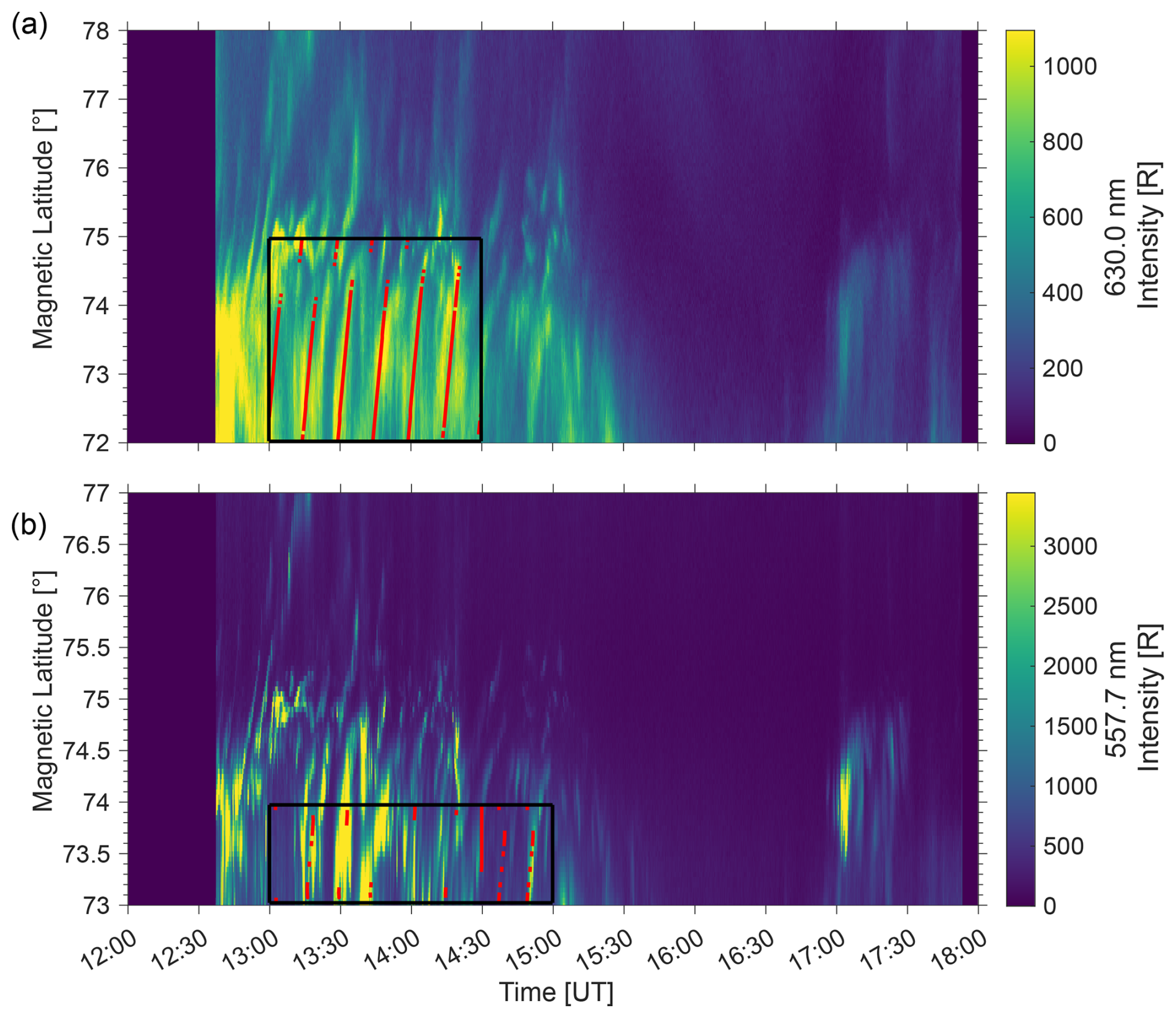
Figure 2 Detection of a UAA event in keograms of both the 630.0 and 557.7 nm channels of the MSP on 16 November 2021. The borders of the detected UAA event (in time and mlat) are shown in black and the reconstructed wavefronts are overlaid in red.

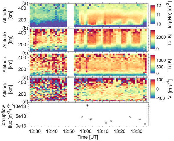
The ESR data are plotted in Fig. 3. The radar was running between 12:27–13:36 UT, except for a short interruption between 12:49 and 12:53 UT. Up to 12:55 UT, the ionosphere was quiet with low electron densities, as shown in Fig. 3a. From 12:55 UT onward, the electron density increases in the E and F-region ionosphere, indicative of particle precipitation. This precipitation is occurring periodically with a period of 10 min, which indicates the presence of UAAs in the radar beam. The precipitation causes the electron temperature (panel b) to increase with the same periodicity. However, no similar increases are visible in the ion temperature (panel c), suggesting a lack of frictional heating and/or Joule heating.

The observed periodicity in the ESR (10 min) is lower than that detected in the MSP (15 min). This is presumably caused by the fact that the localized ESR beam, which is pointing at 75° mlat, is located at the edge of the UAA event. The MSP keogram, Fig. 2a, shows that the auroral arcs at 75° mlat appear slightly more frequently between 13:00–13:30 UT compared to the bulk event around 73.5° mlat. The MSP data in Fig. 2a suggest that the emission intensity range remains constant throughout the wave field with maxima up to 1050 R. We thus assume that the ESR measurements provide a realistic estimation of the event despite its limited beam width.

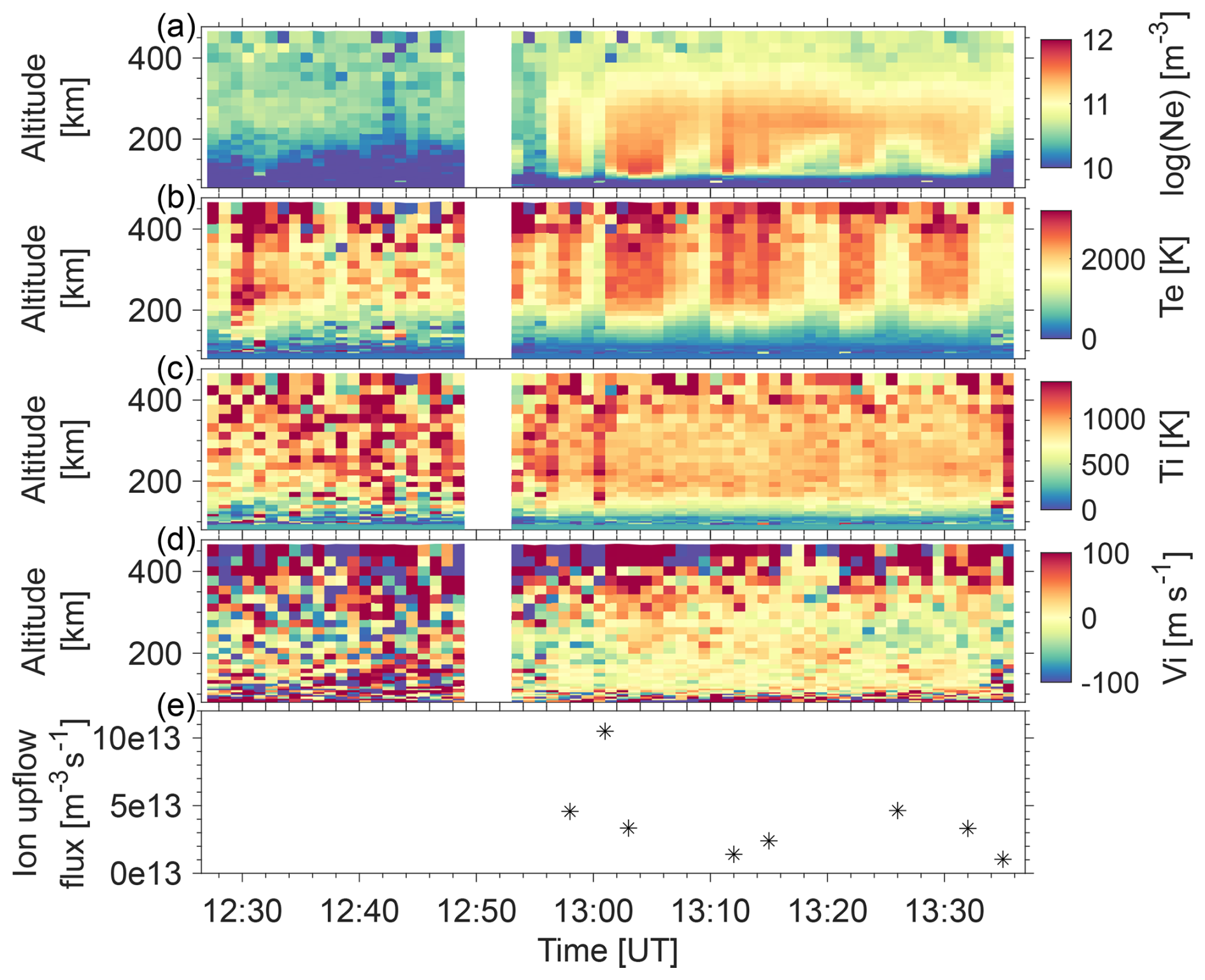
Figure 3 Ionospheric plasma parameters as measured by ESR on 16 November 2021 in panels (a)–(d). Panel (a) shows the logarithmic electron density, panel (b) and (c) the electron and ion temperature respectively, and panel (d) the ion line-of-sight velocity where positive velocities are away from the radar. Panel (e) shows the ion upflow flux calculated using the average electron density and ion velocity between 400–470 km altitude when the upflow criterium from Ogawa et al. (2009) is satisfied.

To further look into the nature of the UAA event, we have analyzed the variation in spectral power and phase with latitude using stations from the IMAGE magnetometer chain. At the wave frequency detected in the MSP, 1.1 mHz, the power and phase variations are shown in Fig. 4a. It can be seen that the spectral power (solid line) has a peak above the HOR (77° geographic latitude (glat); 74° mlat) and HOP (76.5° glat; 73° mlat) magnetometer stations, thus supporting the detection in the MSP between 72–75° mlat. The phase (dashed line) change in Fig. 4a between SOR (70.5° glat; 67.3° mlat) and LYR (78.2° glat; 75.1° mlat) is around 240°. Thus, it exceeds the expected 180° change for a classical FLR (Menk and Waters, 2013). This could be caused by the lack of ground-magnetometer stations between SOR and BJN (74.5° glat; 71.5° mlat). However, the phase change between BJN and HOP is almost zero, while these stations correspond to a steep gradient in spectral power. This indicates that, despite the event showing a clear power peak around HOR and HOP, the UAA event does not have a classic FLR nature. Figure 4b shows the individual power spectra, which are obtained by taking an FFT of the median filtered magnetometer data as shown in Fig. 4c. The individual power spectra show a wider frequency peak between 1.1–2 mHz in HOR and HOP indicating a more complicated dynamics. Magnetometers sense a larger area compared to the MSP, and each station integrates the effects of all currents within its field-of-view into one measurement. This makes it harder to distinguish the UAA signal. In addition, the magnetometers used in this study are located close to the ocean, making their signals sensitive to induced currents in the conducting ocean, which can make up 50 % of the signal (Juusola et al., 2020).

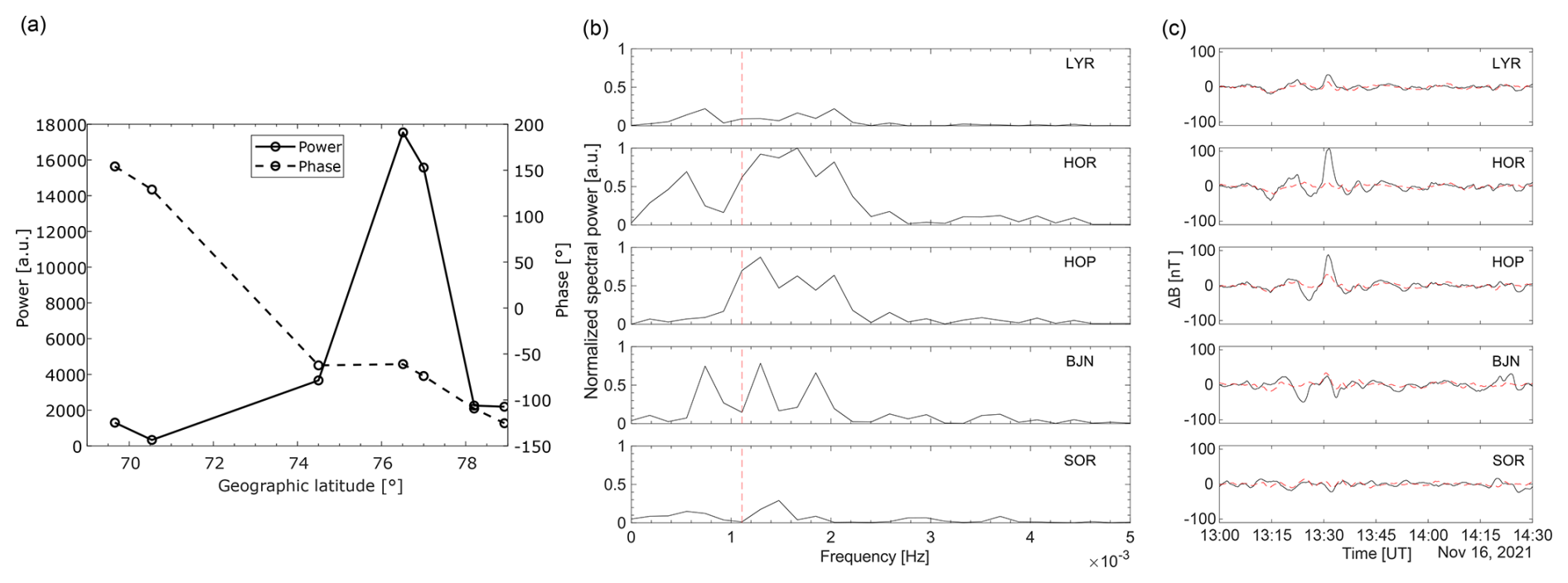
Figure 4 Panel (a): Variation of the spectral power (left y-axis; solid line) and phase (right y-axis; dashed line) at 1.1 mHz between 13:00–14:30 UT using the magnetometer stations TRO, SOR, BJN, HOP, HOR, LYR, and NAL. Panel (b) shows the spectral power between 0–5 mHz for the stations SOR, BJN, HOP, HOR, and LYR, in which the dashed red line indicates the 1.1 mHz frequency. Panel (c) shows the median filtered X (black) and Y (dashed red) components of the corresponding stations.

Figure 3e shows the ion upflow flux when the detection criterion by Ogawa et al. (2009) (i.e. at least three consecutive altitude bins of v_i, shown in Fig. 3d, exceeding 100 m s⁻¹) is satisfied and the flux exceeds 1×10¹³ m⁻² s⁻¹ in order to qualify as ion upflow flux (David et al., 2018). It can be seen that the periodic increases in N_e and T_e are accompanied by ion upflow fluxes ranging between $\mathrm{1}\times {\mathrm{10}}^{\mathrm{13}}-\mathrm{1}\times {\mathrm{10}}^{\mathrm{14}}$ m⁻² s⁻¹, with a median of 3.3×10¹³ m⁻² s⁻¹. One data point suggests the ion upflow to be strong, while the other fluxes fall into the medium and low category. The increased N_e at lower altitudes, indicative of precipitation, in combination with the T_e, and lack of T_i, enhancements suggests the upflow to be of type 2. This fits well with the general ion upflow behavior at 16:00 MLT (magnetic local time) as indicated by Ogawa et al. (2009, Figure 7 herein), which shows that statistically ion upflow at 16 MLT is most likely to occur with only enhancements in T_e. Based on the low geomagnetic activity (Kp=2) we would expect the ion upflow to be low (David et al., 2018).

To investigate whether the ion upflow could result in outflow, the three DMSP overpasses have been studied. DMSP/SSJ energetic electron data are shown in Fig. 5. Panel a indicates that the first overpass (12:57–12:58 UT) occurs on open field lines due to the lack of energetic electron precipitation after 12:57 UT. This overpass is located northeast of Svalbard and thus poleward of our UAA event. The energetic electron precipitation of the second (13:26–13:27 UT) and third (14:38–14:39 UT) overpass, as shown in Fig. 5 b and c, indicates that these overpasses, and thus our UAA event, take place on closed field lines. Densities and ion velocities from the DMSP/SSIES instrument (not shown), however, do not indicate ion outflow signatures for these overpasses. During the period of strongest upflow (around 13:00 UT), we do not have a corresponding DMSP overpass co-located with the UAA event. The co-located overpasses at 13:27 and 14:38 UT indicate that the ion upflow at those times was not strong enough to result in ion outflow.

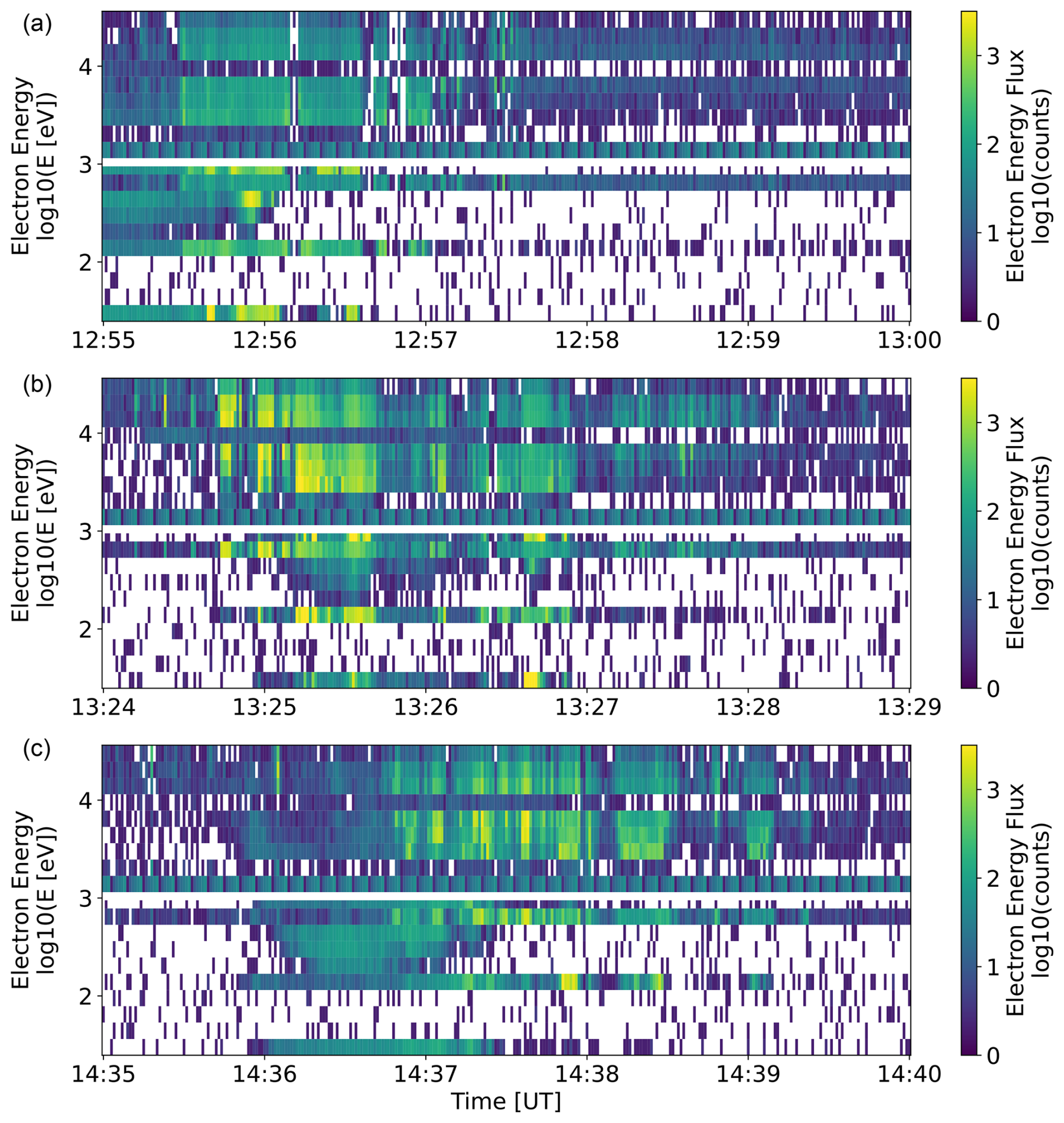
Figure 5 Electron spectrograms from three DMSP/SSJ overpasses between 12:55–13:00 UT (a), 13:24–13:29 UT (b), 14:35–14:40 UT (c). The electron energy flux is plotted as a function of logarithmic electron energy and time.

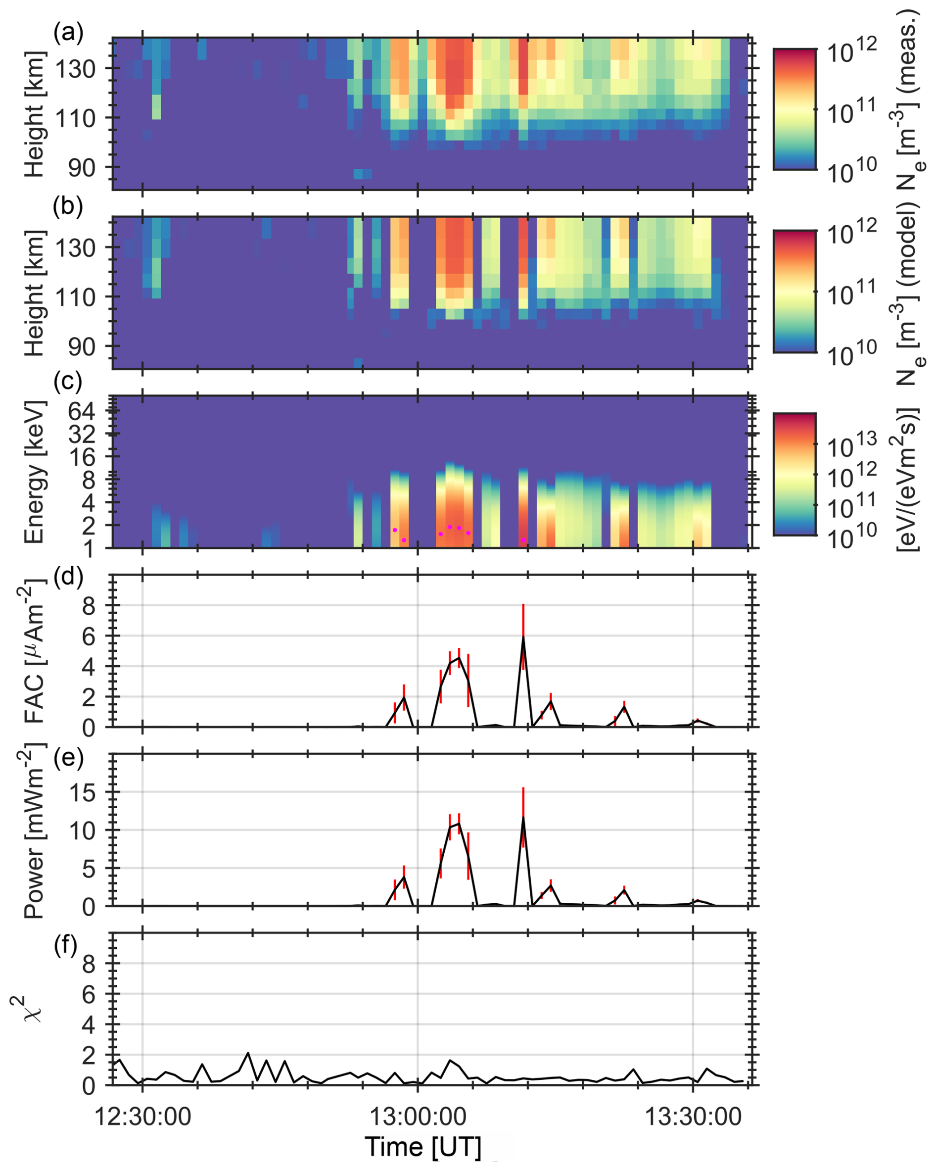
Figure 6 The ELSPEC method which shows: the observed electron density between 80–150 km altitude by the ESR (a), the electron density modeled in the inversion (b), the differential energy flux (c), the upward FACs (d), the total energy flux (e), and the χ² parameter (f). The red bars in (d) and (e) are 1σ error estimates.

FACs give an indication of ongoing energy coupling processes between the magnetosphere and the ionosphere. Both the ELSPEC method, based on EISCAT data, and the Lompe method provide estimates of FACs. However, they do so on different length scales. ELSPEC, as shown in Fig. 6, where panel (d) shows the FAC magnitudes, provides a localized measurement by inverting the EISCAT electron density. The measured value of N_e is depicted in Fig. 6a, while the modeled version is shown in panel (b). Generally, the ELSPEC model underestimates the FAC magnitude, because it only takes electrons with energies above 1 keV into account. The FAC magnitudes in the ELSPEC method range up to 6 µA m⁻². The Lompe method provides a larger-scale overview compared to ELSPEC. In our case, we have chosen the time stamps of the model based on the DMSP overpasses over Svalbard, resulting in three snapshots of which the relevant elements are shown in Fig. 7. The Lompe analysis are based on 5 min windows centered at 12:57, 13:27, and 14:38 UT. The top row of Fig. 7 corresponds to 12:57 UT, the middle row to 13:27 UT, and the bottom row to 14:38 UT. The full snapshots of the inversion can be found in Appendix A. The solutions in the Lompe method are dominated by ground-based magnetometers and Iridium, since there is very little SuperDARN data available in the analysis region, and none around Svalbard. In addition, only the last snapshot, at 14:38 UT, contains a few Swarm data points located at the northern edge of the grid, while for the other snapshots no Swarm data is available. The FACs in the Lompe inversion (Fig. 7a, e, and i; the blue and red color scale shows the FAC magnitudes, where red corresponds to upward and blue to downward FACs), show magnitudes up to ±3 µA m⁻² between 72–75° mlat. At 12:57 UT, Fig. 7a, the ESR beam (at 75° mlat) is located in an upward FAC (red) region, while at 13:27 and 14:38 UT (panels e and i), the ESR beam is located in regions of downward FACs. At these times upward FACs are observed further south in the UAA detection region. This corresponds well with the observed higher FAC values in the ELSPEC method around 13:00 UT. In general, the ELSPEC FAC magnitudes, despite their underestimation, exceed those of Lompe during times of auroral precipitation. Both FAC magnitudes compare well to previously reported values. In case of FLRs, values of 3–6 µA m⁻² (Gillies et al., 2018), 2–3 µA m⁻² (Lotko et al., 1998), up to 5 µA m⁻² (Walker et al., 1992), and 2–4 µA m⁻² (Fenrich et al., 2019) have been reported. For small-scale waves, FAC magnitudes of 1–4 µA m⁻² (Milan et al., 2001) and 0.8 µA m⁻² (Baddeley et al., 2017) have been found. The UAA event thus shows FAC strengths equaling those of FLRs.

Another feature of the FACs in the Lompe method is the alternating direction of the FACs above and just south of Svalbard. This feature is visible in all three Lompe snapshots, but most pronounced at 13:27 UT, as shown in Fig. 7e. The modeled FAC directions in Fig. 7e can be seen directly in an Iridium overpass right over Svalbard providing magnetic field measurements as shown in orange in Appendix A Fig. A1. Similar alternating FAC directionality has previously been observed in combination with a ULF wave event by Fenrich et al. (2019) using data from the SuperDARN radars and the Swarm spacecraft.

Furthermore, the Lompe inversion gives an estimation of the convection velocities. The detection in the MSP shows us that the UAA event is moving with a poleward velocity of around 740 m s⁻¹. This is comparable to the convection velocity in Lompe at 13:27 UT (Fig. 7e; the quiver field). At 12:57 UT (Fig. 7a), Svalbard is on the edge of the two convection cells, making it hard to extract precise velocities, while the convection velocity at 14:38 UT (Fig. 7i), after the detected UAA event has ended, is slightly lower.

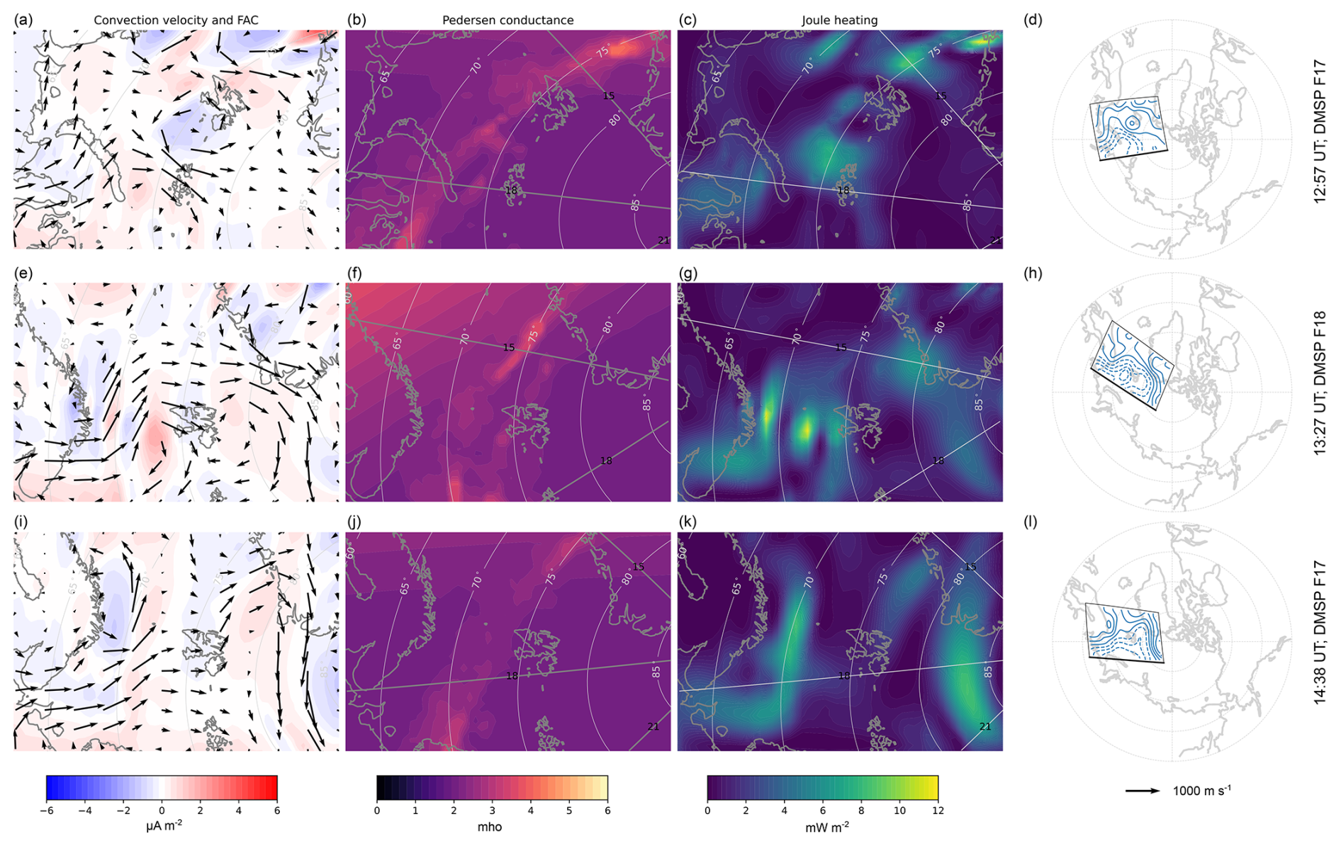
Figure 7 The Lompe inversion at 12:57 UT (top row; panels a–d), 13:27 UT (middle row; panels e–h), and 14:38 UT (bottom row; panels i–l). The first column (panels a, e, and i) shows the convection velocities (quiver field) and the FAC magnitudes (red/blue colormap). The second column (panels b, f, and j) provides the Pedersen conductance, and the third column (panels c, g, and k) the Joule heating. The last column (panels d, h, and l) shows the location of the grid with respect to the magnetic local time and magnetic coordinates. The full data panels of each run are given in Appendix A.

The ELSPEC method, as shown in Fig. 6, also gives an estimation of the total energy flux in the panel e. During the brightest auroral arcs, which take place between 13:00–13:15 UT, the total energy flux goes up to 12 mW m⁻². Outside of this time range, the maximum total energy flux is up to 5 mW m⁻². A similar energy estimate is provided using the DMSP/SSUSI instrument as shown in Fig. 8 for the first two overpasses. Around 12:57 UT, as shown in Fig. 8a, the electron energy flux around Svalbard just exceeds 10 mW m⁻², while it is around 3 mW m⁻² at 13:27 UT. Both the ELSPEC method and the DMSP/SSUSI instrument are thus giving comparable energy dissipation fluxes, showing the strongest energy fluxes around 13:00 UT and weaker fluxes around 13:30 UT. This indicates that the local features captured with the ESR are representative of the larger wavefronts of the UAA event as observed by the DMSP spacecraft. These energy flux magnitudes are comparable to the DMSP/SSUSI fluxes previously reported by Van Hazendonk et al. (2024), which equaled 8–10 mW m⁻² within the ULF wavefronts.

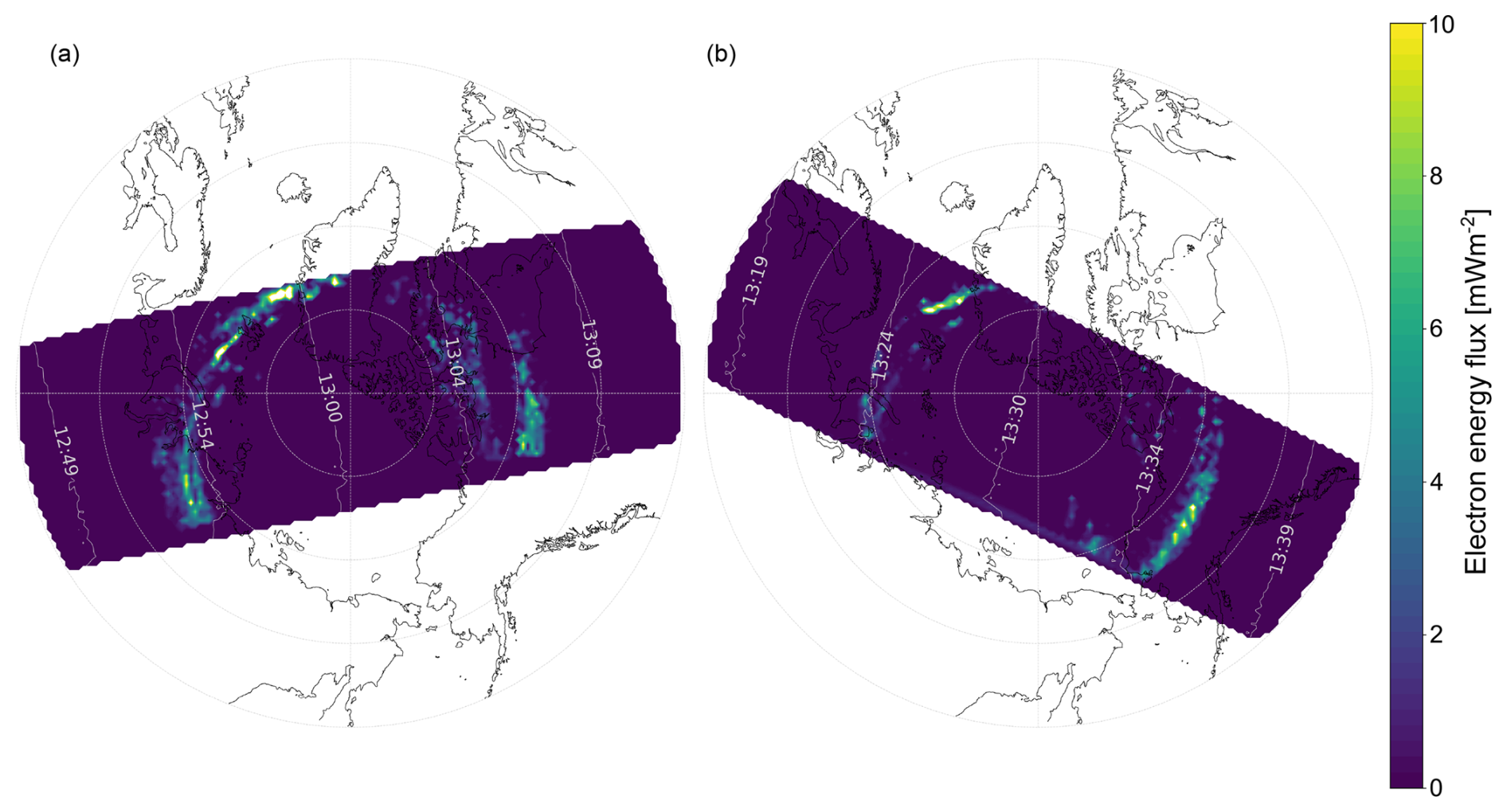
Figure 8 The dissipated electron energy flux measured by the DMSP/SSUSI instrument for overpass 1 (a) and overpass 2 (b).

To investigate how the total energy flux is dissipated, we determined the Joule heating using the Lompe method as shown in Fig. 7c, g, and h. Peak Joule heating rates range between 8–11 mW m⁻². The strongest Joule heating is found in regions between up- and downward FACs, as these areas are characterized by the horizontal Pedersen currents that close the current loops in the ionosphere. In between those regions, Joule heating is limited with base levels between 0.5–2 mW m⁻². The regions with alternating FAC directions, while partly located within the UAA detection region, are mostly found south of the ESR beam. This could explain the lack of T_i enhancements and thus the lack of Joule heating inside the narrow ESR beam. Outside of the ESR beam, the UAA event shows signs of Joule heating as indicated by Lompe. The Joule heating dissipation rates are comparable to those reported previously for ULF wave events with low/intermediate m-numbers and exceed those of high m-number waves as shown in the comparison of Table 1. Comparing to the statistical study by Aikio et al. (2012), our base Joule heating rates fall mostly into the quiet geomagnetic conditions category (Kp: 0–2⁺), thus corresponding well with the observed Kp value of 2, while the peaks indicate high geomagnetic activity (Kp $\ge {\mathrm{5}}^{-}$). This observation is in line with previous findings which showed that the presence of ULF waves increases the dissipation rates above the otherwise expected levels and that ULF waves contribute significantly to the energy budget (Rae et al., 2007; Hartinger et al., 2015; Van Hazendonk et al., 2024).

Van Hazendonk et al. (2024)Hartinger et al. (2015)Rae et al. (2007)Baddeley et al. (2005)Aikio et al. (2012)

Table 1 Previously reported Joule heating dissipation rates. A similar version of this table has been published in Van Hazendonk et al. (2024).

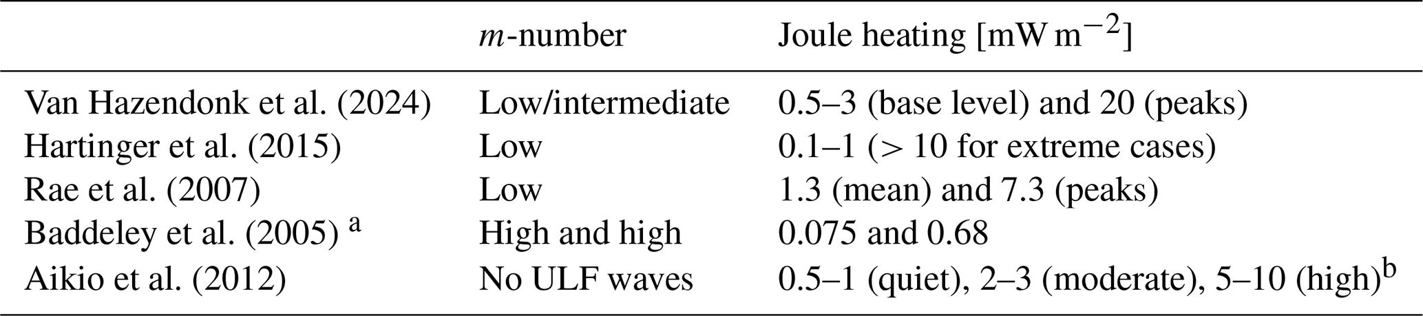
^a Baddeley et al. (2005) present two separate ULF wave events. ^b The rates from Aikio et al. (2012) are median values between 16:00–17:30 MLT. Peak values can be up to double the median values.

4 Discussion

The UAA event on 16 November 2021 13:00–14:30 UT (16:00–17:30 MLT) detected in the MSP is located between 72–75° mlat and has a frequency of 1.1 mHz. Observations in the ESR show the presence of auroral arcs via periodic electron precipitation in the E- and F-region combined with electron temperature increases. Associated with the arcs, type 2 ion upflow is located with predominantly low and medium fluxes. In general, the event shows a complicated dynamics with partly ambiguous observations across different instruments. On one hand, ground-based magnetometers suggest a non-FLR nature and thus indicate small-scale ULF waves. On the other hand, FAC magnitudes, total energy dissipation rates, and Joule heating rates are comparable to previous large-scale, possible FLR-like, events.

The ionospheric ion upflow observed in this paper provides its first direct link to UAAs. Previously, ion outflow has been observed in the inner magnetosphere at lower latitudes during storm time (Chaston et al., 2015). This outflow was connected to kinetic Alfvén waves, and it was hypothesized that simultaneous ionospheric outflow occurred. Our event shows that ionospheric upflow can indeed occur in relation to UAAs, thus fitting within the framework by Chaston et al. (2015). To understand the physical mechanisms explaining the connection between ionospheric ion upflow and UAAs, the model proposed by Samson et al. (2003) and expanded upon by Rankin et al. (2021), gives some insights. This model describes the connection between FACs and the FLR wave field, in which the FLR generates a parallel electric current that is supported by a parallel electric field. This parallel electric field accelerates electrons and ions into the ionosphere causing the UAAs. Based on this model, we expect to observe T_i enhancements in the ESR data, adjacent to the arcs, due to Joule heating caused by the Pedersen currents that close the FAC circuit in the ionosphere. As is seen from figure 3, whilst no T_i enhancements were observed between the arcs, electron density and temperature enhancements are observed, indicating particle acceleration into the ionosphere by a parallel E-field within the arcs.

All in all, the UAA event consists of enough energy input to cause ion upflow, but, based on the ESR data alone, not enough to cause significant Joule heating. This supports that the UAA event consists of smaller-scale ULF waves with a non-FLR nature as also indicated by the ground-based magnetometers. Instead of energy being predominantly deposited via Joule heating, ESR data indicate that part of the dissipated energy went into the acceleration of particles causing N_e and T_e enhancements. Similarly to Van Hazendonk et al. (2024), the kinetic flux might be more important than previously expected. An alternative explanation is that the ESR beam is located too far north to capture the bulk of the Joule heating.

The Lompe model indicates significant Joule heating within the UAA area, as shown in Fig. 7c, g, and k, but locates this Joule heating predominantly south of the ESR beam. These Joule heating rates are comparable to those previously found for large-scale ULF wave events. In our case, however, the Joule heating might be overestimated due to strong dependency on the conductance in the Lompe model. The very limited availability of convection data caused the outputs of the Joule heating and convection velocities to be heavily affected by small changes in conductance. Since the ionospheric currents, J, are mostly based on magnetic field data, an increase in conductance results in a decrease in electric field following Ohm's law: J=ΣE. The E×B drift then results in a reduced convection velocity. We calculated the conductance using Eq. (1), thus depending on the auroral precipitation, solar EUV, and the background conductance. The first term is based on input data from DMSP/SSUSI, while the second one is calculated using well-known empirical formulae as given by Moen and Brekke (1993). The background conductance, however, is a less-known term. Previously, Σ_BG=2 mho has been used (Robinson et al., 2021; Laundal et al., 2025). Recently, Juusola et al. (2025) used long EISCAT time series, both from Tromsø and Svalbard, to determine empirical conductances. The residual of the fit then provided background conductances of ${\mathrm{\Sigma }}_{\mathrm{BG},\mathrm{P}}=\mathrm{0.625}\pm \mathrm{0.008}$ mho and ${\mathrm{\Sigma }}_{\mathrm{BG},\mathrm{H}}=\mathrm{0.894}\pm \mathrm{0.011}$ mho for respectively the Pedersen and Hall background conductances. The ESR data indicate conductances around 0.5 mho before 12:50 UT, while increasing to 1–3 mho in between the auroral arcs during the UAA event. Convection flows are expected to be <1 km s⁻¹ as geomagnetic conditions are quiet. This lead us to use a background conductance of 2 mho, as background conductances ≤1 mho would imply convection flows >1 km s⁻¹, and Joule heating rates up to 25 mW m⁻². The strong dependence of the Joule heating and convection velocity on the background conductance, makes both results less reliable. The comprehensive picture of this event – including both the ESR, DMSP, and Lompe data – thus shows little evidence of large Joule heating especially within the narrow ESR beam. However, it does show enough energy input into the ionosphere to cause particle precipitation and ion upflow.

Furthermore, the input data to the Lompe model in our case mostly comes from ground- and space-based magnetometers. This provides two challenges. Firstly, the Lompe technique implicitly connects all magnetic field perturbations observed by magnetometers within the grid to ionospheric currents within the same grid (Laundal et al., 2022). This might not be true, since magnetometers sense large areas, which can extend across grid boundaries. Secondly, small-scale ULF waves are prone to ionospheric attenuation and thus not always visible in ground-based magnetometer data (e.g. Takahashi et al., 2013). As our event shows a non-FLR signature in the ground-based magnetometer data (Fig. 4), it is likely that the magnetometers, and thus the Lompe method, do not fully capture the ULF wave dynamics. Lastly, it should be noted that the Lompe solutions represent the electrodynamic state over a 5 min window, which is a significant part of the observed ULF wave periodicity of 15 min. As a result, the derived convection and current patterns correspond to an average over a fraction of the ULF wave cycle. This temporal smoothing may reduce the apparent amplitude of rapid variations and should be taken into account when interpreting the relationship between the electrodynamic response and ULF wave periodicities. Shorter time windows for the Lompe models are not feasible due to increased noise due to a reduction in mainly space based measurements and inconsistency of the temporal resolution of Lompe and the conductance as obtained using the DMSP spacecraft. We do therefore believe that the direct observations carry more weight than the outputs of the Lompe model, especially regarding the Joule heating rates and convection velocities.

The observed UAA event has a non-FLR nature, and exhibits small-scale signatures like ionospheric attenuation. This would indicate a generation mechanism internal to the Earth's magnetosphere. On the other hand, FAC magnitudes as provided by ELSPEC and Lompe could indicate larger-scale ULF waves. High solar wind speeds of around 600 km s⁻¹, as shown in Appendix A Fig. A4b, could cause external generation at the Kelvin-Helmholtz instability on the flanks of the magnetopause (Shi et al., 2020; Rae et al., 2005). The solar wind dynamic pressure, shown in Appendix A Fig. A4c, does not indicate that external pressure pulses play a role in the generation. In addition to internal generation mechanisms, phase mixing could contribute to the observed non-FLR nature of the ULF wave event. Characteristically, a FLR shows a narrow resonant frequency peak on the resonant field line that matches eigenfrequency of the wave. Wave growth on adjacent field lines is slower, causing broadening of the peak and phase mixing (Mann et al., 1995; Rankin et al., 2021). Phase mixing can thus redistribute wave energy and change its signature.

The periodic enhancements in both the MSP and ESR as well as the slanted and poleward moving structures in the MSP, indicate the presence of UAAs as explained in Van Hazendonk et al. (2025). However, poleward moving auroral forms (PMAFs) can appear similarly in MSP data (Xing et al., 2012). PMAFs are a dayside phenomena, mostly occurring on open magnetic field lines. However, negative B_y in combination with positive B_z, which is the case for our event as shown in Appendix A Fig. A4a, can cause an asymmetry towards post-noon, making it possible for PMAFs to occur during our event timing (Xing et al., 2012; Yang and Xiang, 2022). However, as discussed earlier, the DMSP/SSJ particle detector data (Fig. 5) show that the UAA event most likely takes place on closed-field lines as indicated by the overpasses at 13:27 and 14:38 UT. We do thus believe that the UAA event takes place on closed field lines and is unlikely to be a PMAF event.

5 Conclusions

In this paper, we presented a comprehensive study of a poleward moving ULF wave driven auroral arc event, utilizing ground-, and space-based instrumentation as well as models. The event takes place on 16 November 2021 between 13:00–14:30 UT (16:00–17:30 MLT) and is located on closed field lines between 72–75° mlat (above Svalbard). Its frequency of 1.1 mHz corresponds to a 15 min periodicity, and the poleward propagation velocity is 740 m s⁻¹. The UAA event provides a strong coupling between the ionosphere and magnetosphere, which is visible through ion upflow, FACs, and energy dissipation. The ion upflow flux falls within the low to medium category with fluxes of around 3.3×10¹³ m⁻² s⁻¹ without proof of outflow. The FACs can locally have magnitudes of at least 6 µA m⁻² as estimated from the ESR electron density measurements. At larger scales the Lompe output gives values around 3 µA m⁻², while also showing the alternating FAC directionality in 2D. The total energy flux peaks at 8 mW m⁻² (large-scale) and 12 mW m⁻² (small-scale), thus showing significant dissipation. Part of this energy is dissipated as kinetic energy via particle acceleration and precipitation as observed in the ESR. No co-located Joule heating was found due to lack of T_i enhancements in the ESR beam, but there is an indication of Joule heating up to 11 mW m⁻² outside this narrow radar beam.

Different measurements provide ambiguous information on the exact nature of the UAA event. On one hand, ground-based magnetometers indicate small-scale waves with a non-FLR nature and the lack of T_i enhancements suggests that most of the UAA energy is deposited via kinetic processes rather than Joule and/or frictional heating as expected for FLRs. On the other hand, FAC magnitudes and energy dissipation rates match those of large-scale, FLR-like events. This shows that the available instrumentation in combination with existing frameworks and models cannot fully capture the complicated UAA dynamics. Phase mixing may play a role in the apparent conflicting observations, in which case the frequency peak of an initial, externally generated-FLR is broadened and the wave exhibits characteristics more aligned with internally driven small-scale wave signatures. Additional instrumentation, such as auroral imaging from space or spatially extended incoherent scatter measurements, could provide more accurate conductivity estimations needed for improved understanding of the ULF wave energy budget and their role in the ionosphere–magnetosphere coupling. Ion upflow should be considered in these future, multi-instrument studies. To the best of our knowledge, this paper now provides the first direct observations of ionospheric ion upflow associated with UAAs.

Appendix A: Additional figures

In this section, the figures containing the full output of the Lompe method are included for the three different snapshots. In addition, the solar wind data is shown.

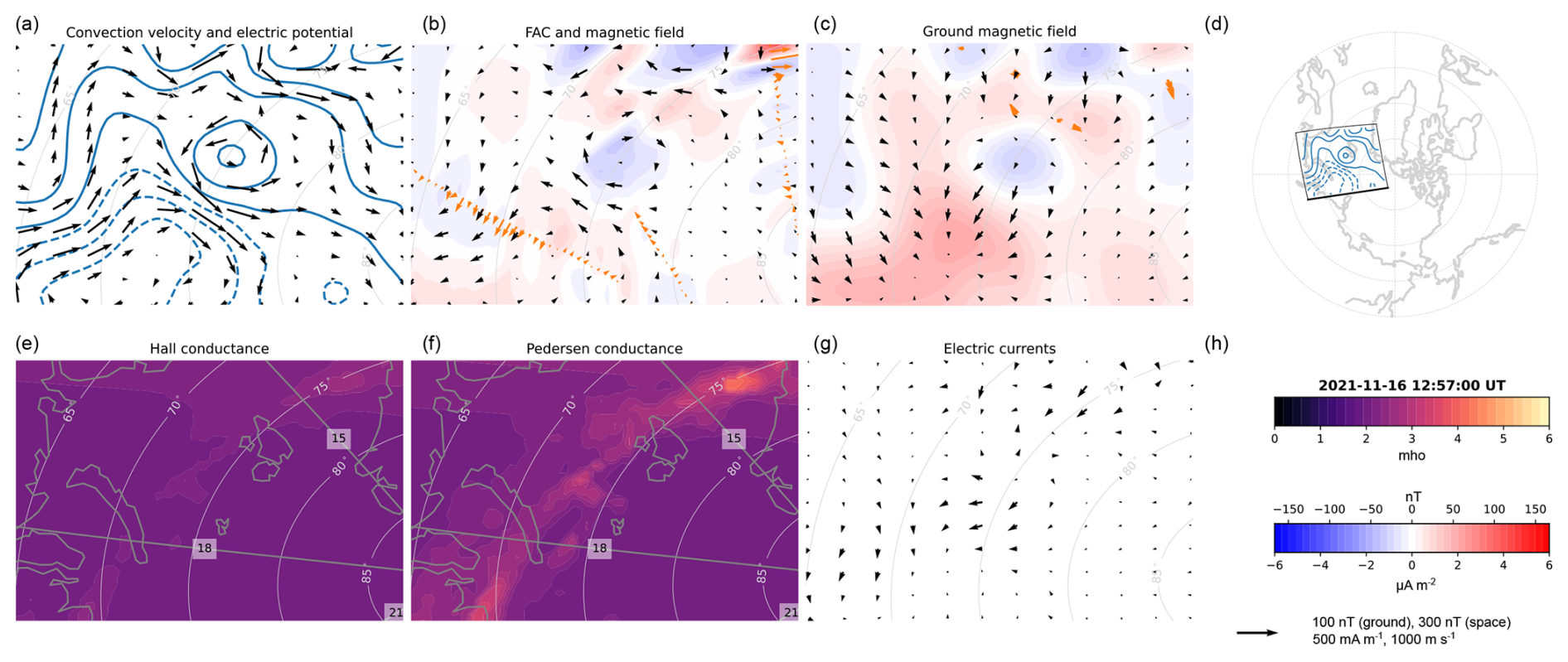
Figure A1 The full Lompe output for the 12:57 UT snapshot. Panel (a) shows the convection velocity (black arrows), and the electric potential contours. Panel (b) depicts the horizontal magnetic field disturbances at 110 km altitude (black arrows), the Iridium horizontal magnetic field measurements (orange arrows), and the FAC densities (color scale). Panel (c) gives the horizontal ground magnetic field perturbations (black arrows), the SuperMAG horizontal magnetic field perturbations in orange, and the radial magnetic field perturbations (color contours). Panel (d) shows the location of the grid with respect to the magnetic local time and magnetic coordinates. Panels (e) and (f) give the Hall and Pedersen conductance, respectively, and panel (g) the horizontal height-integrated ionospheric currents. Panel (h) gives the color and vector scales.

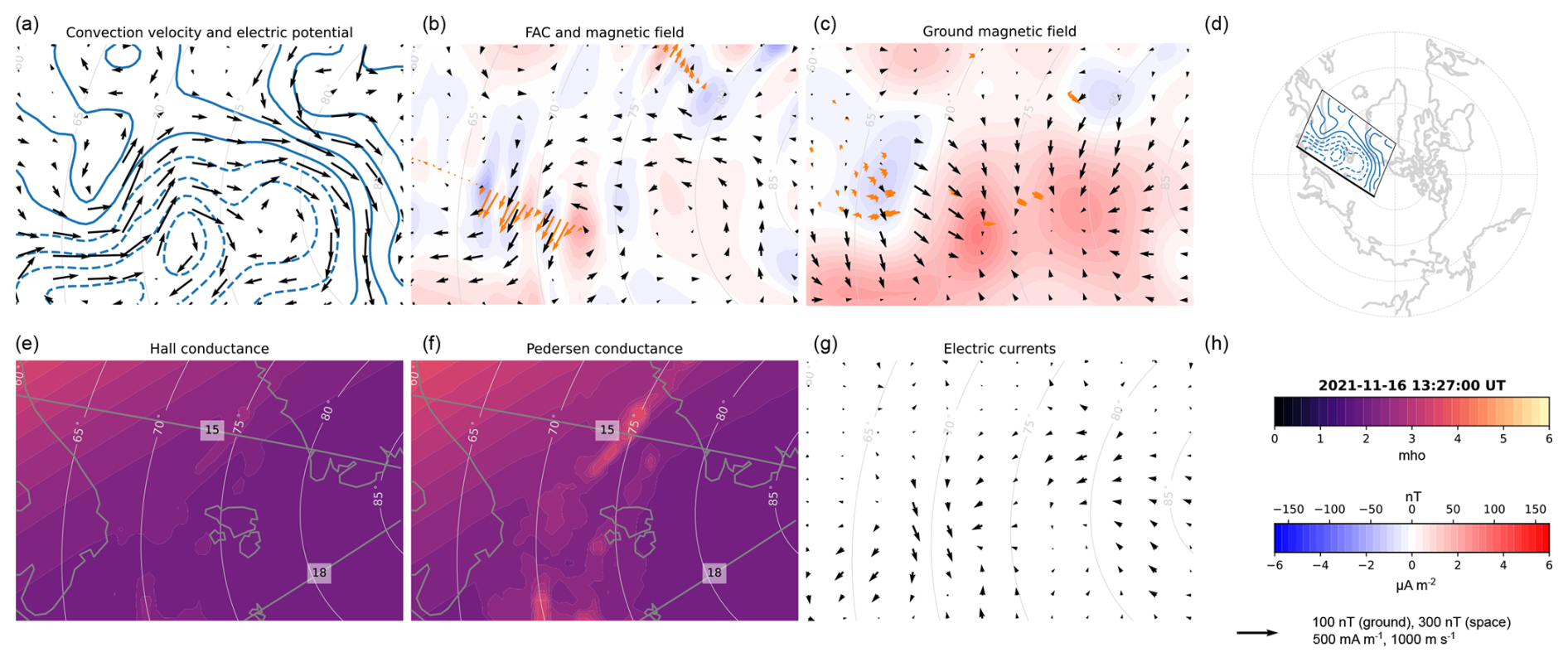
Figure A2 Same as Fig. A1, but for the 13:27 UT snapshot.

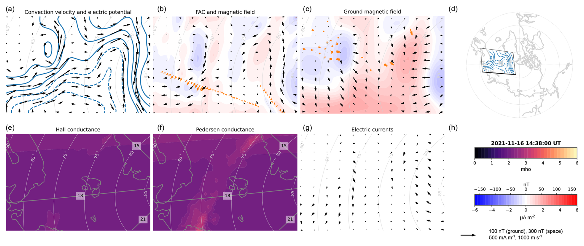
Figure A3 Same as Fig. A1, but for the 14:38 UT snapshot.

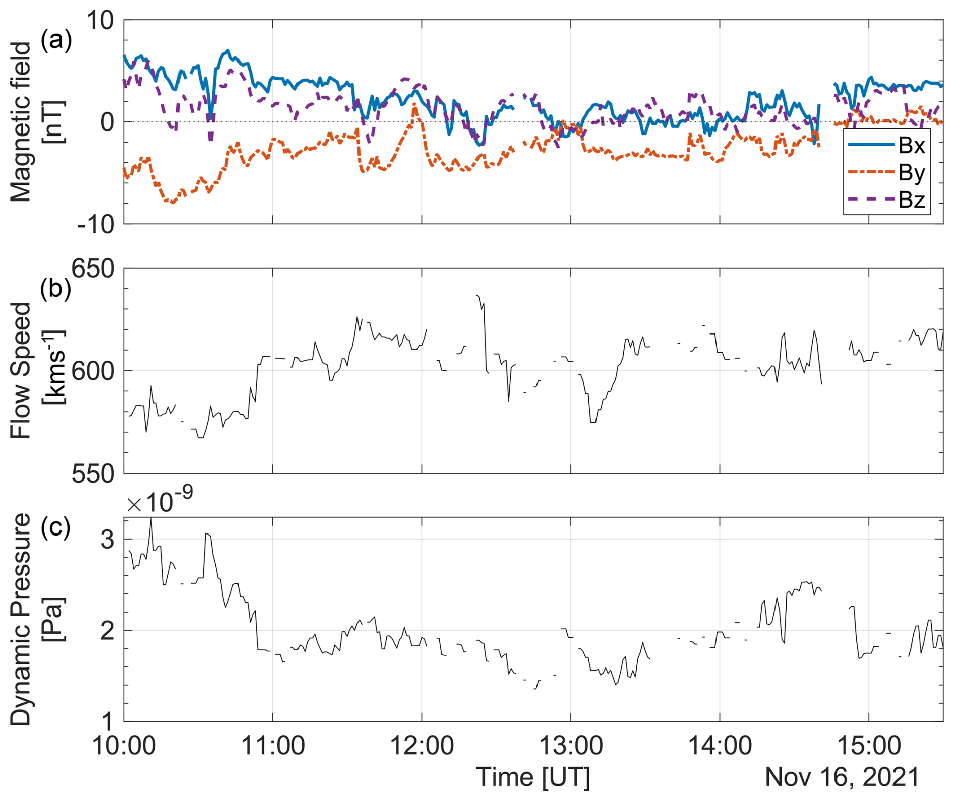
Figure A4 The solar wind data before and during the UAA event. Panel a shows the interplanetary magnetic field, panel b the solar wind velocity, and panel c the solar wind dynamic pressure.