A numerical model for solving the linearized gravity-wave equations by a multilayer method

We developed a numerical model for solving the linearized gravity-wave equations using a multilayer approach that explicitly accounts for viscosity, thermal conduction, and ion drag. The solution strategy is based on a matrix-exponential formalism and comprises two classes of methods: global matrix methods and scattering matrix methods. The model supports both single-frequency waves and time-dependent wave packets. Particular emphasis is placed on the global matrix method, which exploits the structured form of the multilayer system to achieve high computational efficiency while maintaining numerical accuracy. Numerical experiments demonstrate that all methods yield identical accuracy, although the global matrix method is significantly more efficient than the scattering matrix method, especially for time-dependent wave packets. The impact of ion drag on wave characteristics is quantified within this framework. The implementation is freely available as open-source code at https://github.com/AlexandruDoicu/Gravity-Waves (last access: 1 June 2026) and https://doi.org/10.5281/zenodo.21410453 (Doicu and Efremenko, 2026).

1 Introduction

Time-step methods (Liu et al., 2013; Heale et al., 2014; Fritts et al., 2015) are commonly used to solve fully nonlinear sets of governing equations for upper-atmospheric gravity waves, thereby allowing the modeling of wave breaking, secondary wave generation, and weakly nonlinear effects. However, as compared to linear methods for gravity waves (Midgley and Liemohn, 1966; Volland, 1969a, b; Francis, 1973; Yeh and Liu, 1974; Klostermeyer, 1972, 1980; Knight et al., 2024) they are computationally expensive. In Pütz et al. (2019) it was found that a time-step model took several hours to run, while a linear method only took several seconds. In this regard, linear methods are more suitable for analyzing measured data.

The linearized equations can be transformed into a linear system of ordinary differential equations with variable coefficients that depend on the background atmospheric parameters and their height derivatives. (The atmospheric parameters are assumed to be horizontally uniform but vertically varying.) A common technique for integrating the linearized equations is the multilayer method first applied by Pfeffer and Zarichny (1962). In this method, the atmosphere is divided into a sequence of thin layers, and in each layer, a linear system of ordinary differential equations with constant coefficients is solved. The analytic wave solutions in neighboring layers are matched by the continuity condition of the variables across the interface. There are two methods for deriving a linear system of ordinary differential equations with constant coefficients. These approaches are referred to as the physical multilayer method and the numerical multilayer method. It is worth noting that Hines (1973) used the terms standard and nonstandard multilayer methods, respectively, for these two approaches.

1. In the physical multilayer method, the atmospheric parameters, and in particular, the temperature and wind velocity, are assumed to be constant within each layer (Midgley and Liemohn, 1966; Volland, 1969a, b; Francis, 1973; Yeh and Liu, 1974). As a result of the piecewise constant approximation, the height derivatives of the atmospheric parameters are zero within each layer.

2. In the numerical multilayer method, the coefficients as a whole are approximated by their values in the middle of the layer (Klostermeyer, 1972). As a result, the height derivatives of the atmospheric parameters (approximated by their values in the middle of the layers) are also included in the resulting system of equations.

The criticism of physical multilayer methods by Hines (1973) concerns whether the equations describing the state variables in a layer are physically realistic. He concluded that it is impossible to find the appropriate variables when either (i) the viscosity and the wind velocity are nonzero or (ii) the thermal conductivity and the temperature height derivative are nonzero. However, as mentioned by Knight et al. (2022), Hines' concern about the physical meaning of the state variables is not relevant for a numerical multilayer method. The reason is that in a purely mathematical context, it is sufficient to prove that the method, converges to a correct solution in the infinitesimally thin layer limit. A justification of this result, based on a matrix–exponential representation for the solution, can be found in Klostermeyer (1980).

According to Volland (1969a), a layer is said to be isothermal if the background temperature is constant, and homogeneous if the kinematic viscosity is constant. In the simplified windless-atmosphere model considered by Midgley and Liemohn (1966); Volland (1969a, b); Francis (1973); Yeh and Liu (1974), the gradients of the background temperature and kinematic viscosity are neglected. In this case, the dispersion relation, associated to the system of ordinary differential equations, separates into three pairs of ascending and descending gravity-wave, viscosity-wave, and thermal conduction-wave modes. The viscosity-wave and thermal conduction-wave modes are also referred to as dissipative modes. The main distinction between the two pairs of dissipative modes and the pair of gravity-wave modes is that the latter have smaller vertical wavenumber imaginary parts. This means that ascending gravity-wave modes do not decrease in amplitude as rapidly with increasing altitude as dissipative modes. On the other hand, the assumption of locally constant kinematic viscosity is unrealistic as discussed in Knight et al. (2019). If one assumes instead that the dynamic viscosity is constant within each layer, it is generally not possible to distinguish between ascending and descending modes for certain wavenumbers, frequencies, and background parameters (Knight et al., 2022, 2019, 2021). In this context, Knight et al. (2022) explained that the problem of distinguishing ascending from descending modes is related to the problematic branch points of the root functions giving the vertical wavenumber as a function of complex frequency. Along this line, the authors proposed a technique called imaginary frequency shift to assist in achieving this separation.

The inclusion of dissipative modes in a linearized model produces a numerical swamping (Maeda, 1985) in which certain descending modes grow so rapidly in the upward direction that numerical overflow occurs when the system of differential equation is subject to lower and upper boundary conditions. Several methods have been proposed to reduce numerical swamping.

1. Midgley and Liemohn (1966) employed an iterative method that can be regarded as a Gauss–Seidel group iteration. However, the Gauss–Seidel iteration may fail to converge in certain situations, in particular when gravity and dissipative modes become strongly coupled, as discussed in Volland (1969a, b). Klostermeyer (1980) avoids this difficulty by introducing the concept of a transfer matrix, which relates the wave amplitudes at different altitude levels and provides a more robust framework for treating such coupling.

2. Volland (1969b) applied the scattering matrix formalism to a three-layer atmosphere assuming (i) abrupt changes in variables at the interfaces between the different layers and (ii) that certain background parameters remain constant in the lower and upper layers. Knight et al. (2019) also formulated the problem in terms of scattering matrices which are closely related to the reflection and transmission matrices appearing in seismology (Pérez-Álvarez and García-Moliner, 2004). However, in contrast to Volland, the authors used a more rigorous approach, i.e., a sequence of composed scattering matrices instead of just a one stand-alone scattering matrix.

3. Maeda (1985) defined numerical swamping as the annihilation of linear independence among supposedly independent solutions. To address this challenge and obtain a comprehensive set of special solutions that are linearly independent, he utilized a technique developed by Inoue and Horowitz (1966).

In radiative transfer, it is also necessary to solve a linear system of ordinary differential equations with constant coefficients. This arises by transforming the continuous dependence of radiance on direction into a dependence on a discrete set of directions. The standard methods for solving the linear system of ordinary differential equations are the discrete ordinate method (Stamnes, 1986; Wick, 1943; Chandrasekhar, 1960; Stamnes and Swanson, 1981) and the matrix operator method (Plass et al., 1973; Kattawar et al., 1973; van de Hulst, 1963; Nakajima and Tanaka, 1986). In the classical discrete ordinate method, the solution to these equations is expressed as a linear combination of characteristic solutions of the discretized problem. Conversely, the matrix operator method focuses on numerical computations of reflection and transmission matrices. Both methods can be formulated using the matrix exponential formalism. In the framework of the so called discrete ordinate method with matrix exponential, Doicu and Trautmann (2009a, b) designed stable numerical algorithms for computing the radiance field in a multi-layered atmosphere, while in the framework of the matrix operator method with matrix exponential, Budak et al. (2011, 2012) provided explicit and stable representations for the reflection and transmission matrices. A consistent overview of the matrix exponential description of radiative transfer can be found in Efremenko et al. (2017).

The main purpose of this article is to apply radiative transfer techniques to solve the linearized gravity-wave equations. As a prototype, we will consider the equations that describe gravity waves in the ionosphere, and that include viscosity, thermal conduction, and ion drag. In principle, a full wave model for the ionosphere comprises the hydrodynamic equations for the neutral atmosphere and the ionospheric equations. These two sets of equations are coupled through the ion drag, and should be solved together. However, to simplify the analysis, we decouple the two sets of equations by adopting a fast field-aligned diffusion approximation, which may be viewed as a generalization of an approximation originally proposed by Klostermeyer (1972).

Our paper is organized as follows. In Sect. 2, we present the derivation of the matrix exponential solution of the linearized equations, while Sect. 3 describes stable numerical methods for computing the complex amplitudes (hereafter referred to simply as amplitudes) of the characteristic solution in a stratified atmosphere. Section 4, which is largely inspired by the works of Knight et al. (2019, 2021, 2022, 2024), addresses the computation of the perturbed quantities for both harmonic and non-harmonic source functions, that is, for single-frequency waves and time-dependent wave packets. The concepts of causality and the imaginary frequency shift, which are rigorously treated in Knight et al. (2019, 2021, 2022), are also briefly discussed. Aspects of the numerical implementation are addressed in Sect. 5, and representative simulation results are presented in Sect. 6. Additional theoretical issues are discussed in the Appendices. Appendix A contains the linearized hydrodynamic equations for the neutral atmosphere and the derivation of the underlying system of differential equations. Appendix B outlines the linearized ionospheric equations and discusses the assumptions employed to decouple the hydrodynamic and ionospheric systems. Appendix C describes methods for computing grid-point values of the state vector in a stratified atmosphere. Appendix D addresses several implementation issues, including a practical, albeit heuristic, approach for determining the imaginary frequency shift.

2 Matrix exponential solution of the linearized equations

To design a full wave model for the ionosphere, we use the hydrodynamic equations for the neutral atmosphere and the ionospheric equations. In a linearized (perturbation) method, a quantity f is expressed as

$$\begin{array}{}\text{(1)}& f=f_{\mathrm{0}}+f^{\prime },\end{array}$$

where f₀ and f^′ are the unperturbed (background) and the perturbed quantity, respectively. The perturbations are assumed to be small so that it is justified to neglect all terms of higher than the first order.

Concretely, we solve the linearized hydrodynamic equations for the neutral atmosphere together with the linearized ion continuity and momentum equations. The linearized neutral-atmosphere equations are solved under the following assumptions:

• A1.

  The geographic and geomagnetic coordinates are identical.

• A2.

  The wave propagates in the meridional plane (the x-coordinate is positive southwards while the z-coordinate is positive upwards), i.e.,

  $$\begin{array}{}\text{(2)}& f=f(x,z,t).\end{array}$$
• A3.

  All background (unperturbed) quantities vary only in the z-direction, i.e.,

  $$\begin{array}{}\text{(3)}& f_{\mathrm{0}}=f_{\mathrm{0}}\left(z\right),\end{array}$$

  while all perturbations vary harmonically in time and the x-direction, i.e.,

  $$\begin{array}{}\text{(4)}& f^{\prime }=f^{\prime }(x,z,t)=\stackrel{\mathrm{‾}}{f}\left(z\right){\mathrm{e}}^{\mathrm{j}(\mathit{\omega }t-k_{x}x)},\end{array}$$

  where ω is the angular frequency and k_x the horizontal wavenumber. Note that in some gravity-wave studies, the opposite sign convention for frequency and horizontal wavenumber is used (e.g. Knight et al., 2025).

The linearization model is described in Appendix A. It provides a general framework that accounts for the altitude derivatives of the background velocity u₀, temperature T₀, density scale height H_ρ, and dynamic viscosity μ₀. Apart from the ion-drag terms, the formulation follows a structure similar to those employed by Vadas and Nicolls (2012) and Knight et al. (2024).

The computation of the ion-drag force and ion-drag heating is presented in Appendix B. The ion-drag terms are introduced in an approximate manner, with the explicit aim of decoupling the hydrodynamic and ion equation systems. To this end, we adopt the following assumptions:

• B1.

  In the ion continuity equation, the perturbed production and loss terms are neglected.

• B2.

  In the ion momentum equation, ion inertia and ion–ion collisions are neglected, and only transport parallel to the magnetic field lines is retained. Under these assumptions, the ion momentum equation reduces to the ambipolar diffusion equation.

• B3.

  To decouple the ion continuity equation from the diffusion equation, fast field-aligned diffusion is assumed, meaning that the field-aligned diffusion is sufficiently strong for the relative ion perturbation and the perturbed diffusion velocity to remain nearly constant along a magnetic field line.

The linearized equations lead to a linear system of ordinary differential equations, written in matrix form as

$$\begin{array}{}\text{(5)}& {\displaystyle \frac{\mathrm{1}}{k_x}}{\displaystyle \frac{\mathrm{d}\mathit{e}}{\mathrm{d}z}}=\mathbf{A}\mathit{e},\end{array}$$

where

$$\begin{array}{}\text{(6)}& \mathit{e}=[\widehat{u},\widehat{w},\widehat{T},\widehat{\mathcal{U}},\widehat{\mathcal{W}},\widehat{\mathcal{T}}{]}^T\end{array}$$

is the state vector, and A is the propagation matrix with altitude-independent elements within a thin atmospheric layer (whose expressions follow from Eqs. A41–A46 of Appendix A). In general, the unknowns (the hat quantities in Eq. 6) are defined through the relation

$$\begin{array}{}\text{(7)}& \stackrel{\mathrm{‾}}{f}\left(z\right)=C\left(z\right)\widehat{f}\left(z\right),\end{array}$$

where $\stackrel{\mathrm{‾}}{f}$ is defined by Eq. (4), and C is a known quantity that ensures that $\widehat{f}$ is dimensionless and that may or may not depend on altitude (here, we indicate that C depend on z). Specifically, for the background velocity ${\mathit{u}}_{\mathrm{0}}=(u_{\mathrm{0}},\mathrm{0},\mathrm{0})$, and the perturbed velocity ${\mathit{u}}^{\prime }=(u^{\prime },\mathrm{0},w^{\prime })$, we have (cf. Eqs. A39 and A40 of Appendix A)

$$\begin{array}{}\text{(8)}& {\displaystyle }\stackrel{\mathrm{‾}}{u}\left(z\right)& {\displaystyle }={\displaystyle \frac{{\mathit{\omega }}_{\mathrm{0}}}{k_x}}\widehat{u}\left(z\right),\text{(9)}& {\displaystyle }\stackrel{\mathrm{‾}}{w}\left(z\right)& {\displaystyle }={\displaystyle \frac{{\mathit{\omega }}_{\mathrm{0}}}{k_x}}\widehat{w}\left(z\right),\text{(10)}& {\displaystyle }\stackrel{\mathrm{‾}}{T}\left(z\right)& {\displaystyle }=T_{\mathrm{0}}\left(z\right)\widehat{T}\left(z\right),\end{array}$$

and

$$\widehat{\mathcal{U}}={\displaystyle \frac{\mathrm{d}\widehat{u}}{\mathrm{d}z}},\widehat{\mathcal{W}}={\displaystyle \frac{\mathrm{d}\widehat{w}}{\mathrm{d}z}},\widehat{\mathcal{T}}={\displaystyle \frac{\mathrm{d}\widehat{T}}{\mathrm{d}z}}.$$

where ω₀ is a reference frequency.

If (λ_n,v_n) is an eigenpair of the matrix A, i.e., Av_n=λ_nv_n for $n=\mathrm{1},\mathrm{\dots },N$, where N=dim(e), the general solution of Eq. (5) is a linear combination of the characteristic solutions exp (k_xλ_nz)v_n, that is,

$$\begin{array}{ll}{\displaystyle }\mathit{e}\left(z\right)& {\displaystyle }=\sum _{n=\mathrm{1}}^N{a}_n{\mathrm{e}}^{k_x{\mathit{\lambda }}_{n}z}{\mathit{v}}_n\\ {\displaystyle }& {\displaystyle }=\left[{\mathit{v}}_{\mathrm{1}},\mathrm{\dots }{\mathit{v}}_N\right]\left[\begin{array}{ccc}{\mathrm{e}}^{k_x{\mathit{\lambda }}_{\mathrm{1}}z}& \mathrm{\cdots }& \mathrm{0}\\ \mathrm{⋮}& \mathrm{\ddots }& \mathrm{⋮}\\ \mathrm{0}& \mathrm{\cdots }& {\mathrm{e}}^{k_x{\mathit{\lambda }}_{N}z}\end{array}\right]\left[\begin{array}{c}{a}_{\mathrm{1}}\\ \mathrm{⋮}\\ a_N\end{array}\right]\\ \text{(11)}& {\displaystyle }& {\displaystyle }=\mathbf{V}\text{diag}\left[{\mathrm{e}}^{k_x{\mathit{\lambda }}_{n}z}\right]\mathit{a},\end{array}$$

where

$$\begin{array}{}\text{(12)}& \mathbf{V}=[{\mathit{v}}_{\mathrm{1}},\mathrm{\dots },{\mathit{v}}_N],\text{diag}\left[{\mathrm{e}}^{k_x{\mathit{\lambda }}_{n}z}\right]=\left[\begin{array}{ccc}{\mathrm{e}}^{k_x{\mathit{\lambda }}_{\mathrm{1}}z}& \mathrm{\cdots }& \mathrm{0}\\ \mathrm{⋮}& \mathrm{\ddots }& \mathrm{⋮}\\ \mathrm{0}& \mathrm{\cdots }& {\mathrm{e}}^{k_x{\mathit{\lambda }}_{N}z}\end{array}\right],\end{array}$$

and $\mathit{a}=[a_{\mathrm{1}},\mathrm{\dots },a_N{]}^T$. At z=0, we have e(0)=Va; thus,

$$\begin{array}{}\text{(13)}& \mathit{a}={\mathbf{V}}^{-\mathrm{1}}\mathit{e}\left(\mathrm{0}\right),\end{array}$$

implying (cf. Eq. 11),

$$\begin{array}{}\text{(14)}& \mathit{e}\left(z\right)=\mathbf{V}\text{diag}\left[{\mathrm{e}}^{k_x{\mathit{\lambda }}_{n}z}\right]{\mathbf{V}}^{-\mathrm{1}}\mathit{e}\left(\mathrm{0}\right)={\mathrm{e}}^{k_x\mathbf{A}z}\mathit{e}\left(\mathrm{0}\right),\end{array}$$

and conversely,

$$\begin{array}{}\text{(15)}& \mathit{e}\left(\mathrm{0}\right)=\mathbf{V}\text{diag}\left[{\mathrm{e}}^{-k_x{\mathit{\lambda }}_{n}z}\right]{\mathbf{V}}^{-\mathrm{1}}\mathit{e}\left(z\right)={\mathrm{e}}^{-k_x\mathbf{A}z}\mathit{e}\left(z\right).\end{array}$$

From the theory of gravity waves within an isothermal, nondissipative atmosphere, it is generally known that the amplitude of an ascending modes increases like $\exp [z/(\mathrm{2}{H}_{\text{a}}\left)\right]$, where H_a is the atmospheric scale height (Hines, 1960). This is necessary to keep the wave energy constant in an atmosphere where the pressure decreases exponentially with height. In this regard, we define the vertical wavenumber k_zn through the relation

$$\begin{array}{}\text{(16)}& \text{diag}\left[{\mathrm{e}}^{k_x{\mathit{\lambda }}_{n}z}\right]=\text{diag}\left[{\mathrm{e}}^{z/\left(\mathrm{2}{H}_{\text{a}}\right)}{\mathrm{e}}^{-\mathrm{j}{k}_{zn}z}\right],\end{array}$$

yielding

$$\begin{array}{}\text{(17)}& {\mathit{\lambda }}_n=-{\displaystyle \frac{\mathrm{j}}{k_x}}{k}_{zn}+{\displaystyle \frac{\mathrm{1}}{\mathrm{2}}}\mathit{\alpha },\end{array}$$

and conversely,

$$\begin{array}{}\text{(18)}& k_{zn}=\mathrm{j}{k}_x\left({\mathit{\lambda }}_n-{\displaystyle \frac{\mathrm{1}}{\mathrm{2}}}\mathit{\alpha }\right),\end{array}$$

where $\mathit{\alpha }=\mathrm{1}/\left(k_x{H}_{\text{a}}\right)$. The characteristic equation $\text{det}(\mathbf{A}-\mathit{\lambda }{\mathbf{I}}_N)=\mathrm{0}$ has N=6 solutions. As shown in Appendix A, for a constant kinematic viscosity the solutions occur in pairs and correspond to (i) ascending and descending gravity-wave modes, (ii) ascending and descending viscosity-wave modes, and (iii) ascending and descending thermal-conduction wave modes (Volland, 1969b; Francis, 1973). In that appendix, this pairing is explicitly demonstrated by deriving the dispersion relation for the special case of an isothermal (constant background temperature), homogeneous (constant kinematic viscosity), and windless atmosphere without ion drag. This solution classification is made according to the imaginary part of the vertical wavenumber k_zn. In the more realistic case of a constant background dynamic viscosity, it is generally not possible to define ascending and descending modes as corresponding pairs (see Eq. A52 in Appendix A). However, in our model we will use the same rule as in the case of a homogeneous atmosphere, even though the traditional concept of classifying waves in pairs is no longer applicable. Specifically, we compute k_zn for $n=\mathrm{1},\mathrm{\dots },N$ by means of Eq. (18), and order the set $\mathit{\{}{k}_{zn}{\mathit{\}}}_{n=\mathrm{1}}^N$, and accordingly, $\mathit{\{}{\mathit{\lambda }}_n{\mathit{\}}}_{n=\mathrm{1}}^N$, such that

$$\begin{array}{}\text{(19)}& \begin{array}{rl}\text{Im}\left(k_{z\mathrm{3}}\right)& \le \text{Im}\left(k_{z\mathrm{2}}\right)\le \text{Im}\left(k_{z\mathrm{1}}\right)\le \text{Im}\left(k_{z\mathrm{4}}\right)\\ & \le \text{Im}\left(k_{z\mathrm{5}}\right)\le \text{Im}\left(k_{z\mathrm{6}}\right).\end{array}\end{array}$$

By convention, (i) the pairs $(k_{z\mathrm{1}}=k_{z\mathrm{1}}^{+},{\mathit{\lambda }}_{\mathrm{1}}={\mathit{\lambda }}_{\mathrm{1}}^{+})$ and $(k_{z\mathrm{4}}=k_{z\mathrm{1}}^{-},{\mathit{\lambda }}_{\mathrm{4}}={\mathit{\lambda }}_{\mathrm{1}}^{-})$ will correspond to ascending and descending gravity-wave modes, respectively, (ii) the pairs $(k_{z\mathrm{2}}=k_{z\mathrm{2}}^{+},{\mathit{\lambda }}_{\mathrm{2}}={\mathit{\lambda }}_{\mathrm{2}}^{+})$ and $(k_{z\mathrm{5}}=k_{z\mathrm{2}}^{-},{\mathit{\lambda }}_{\mathrm{5}}={\mathit{\lambda }}_{\mathrm{2}}^{-})$ to ascending and descending viscosity-wave modes, respectively, and (iii) the pairs $(k_{z\mathrm{3}}=k_{z\mathrm{3}}^{+},{\mathit{\lambda }}_{\mathrm{3}}={\mathit{\lambda }}_{\mathrm{3}}^{+})$ and $(k_{z\mathrm{6}}=k_{z\mathrm{3}}^{-},{\mathit{\lambda }}_{\mathrm{6}}={\mathit{\lambda }}_{\mathrm{3}}^{-})$ to ascending and descending thermal conduction-wave modes, respectively. Thus, the vertical wavenumber is an auxiliary quantity that is used only to identify the different modes. According to the notation introduced above, $\mathit{\{}{\mathit{\lambda }}_m^{+}{\mathit{\}}}_{m=\mathrm{1}}^M,$ where $M=N/\mathrm{2}$ is the number of modes, is the set of eigenvalues defining ascending modes, and $\mathit{\{}{\mathit{\lambda }}_m^{-}{\mathit{\}}}_{m=\mathrm{1}}^M$ is the set of eigenvalues defining descending modes. Because $\mathrm{Re}\left({\mathit{\lambda }}_n\right)=\text{Im}\left(k_{zn}\right)/k_x+\mathit{\alpha }/\mathrm{2}$, it is obvious that we can put aside the concept of vertical wavenumber when identifying the different wave modes. We can simply order the set $\mathit{\{}{\mathit{\lambda }}_n{\mathit{\}}}_{n=\mathrm{1}}^N$, such that

$$\begin{array}{}\text{(20)}& \begin{array}{rl}\mathrm{Re}\left({\mathit{\lambda }}_{\mathrm{3}}\right)& \le \mathrm{Re}\left({\mathit{\lambda }}_{\mathrm{2}}\right)\le \mathrm{Re}\left({\mathit{\lambda }}_{\mathrm{1}}\right)\le \mathrm{Re}\left({\mathit{\lambda }}_{\mathrm{4}}\right)\\ & \le \mathrm{Re}\left({\mathit{\lambda }}_{\mathrm{5}}\right)\le \mathrm{Re}\left({\mathit{\lambda }}_{\mathrm{6}}\right),\end{array}\end{array}$$

and use the same classification rule as above. A commonly cited interpretation of condition (20) is that, for increasing z, the exponential term exp(k_xλ_nz) will tend to be damped more for ascending modes than for descending modes; conversely, for decreasing z, the roles of ascending and descending modes are reversed. However, such a classification of upgoing and downgoing roots (e.g., Volland, 1969b and related works) was primarily heuristic and lacked a rigorous theoretical justification. By contrast, the approach of Knight et al. (2019), which is discussed in Sect. 4, introduces additional constraints beyond condition (20) that are explicitly related to causality and is therefore grounded in theoretical considerations rather than heuristic arguments.

To highlight the different wave modes, we organize the state vector e(z) as

$$\begin{array}{ll}{\displaystyle }& {\displaystyle }\mathit{e}\left(z\right)={\mathit{e}}_{+}\left(z\right)+{\mathit{e}}_{-}\left(z\right)\\ {\displaystyle }& {\displaystyle }=\left(\sum _{m=\mathrm{1}}^M{a}_m^{+}{\mathrm{e}}^{k_x{\mathit{\lambda }}_m^{+}z}{\mathit{v}}_m^{+}\right)+\left(\sum _{m=\mathrm{1}}^M{a}_m^{-}{\mathrm{e}}^{k_x{\mathit{\lambda }}_m^{-}z}{\mathit{v}}_m^{-}\right)\\ \text{(21)}& {\displaystyle }& {\displaystyle }=[{\mathbf{V}}_{+},{\mathbf{V}}_{-}]\left[\begin{array}{cc}\text{diag}\left[{\mathrm{e}}^{k_x{\mathit{\lambda }}_m^{+}z}\right]& {\mathbf{0}}_M\\ {\mathbf{0}}_M& \text{diag}\left[{\mathrm{e}}^{k_x{\mathit{\lambda }}_m^{-}z}\right]\end{array}\right]\left[\begin{array}{c}{\mathit{a}}_{+}\\ {\mathit{a}}_{-}\end{array}\right],\end{array}$$

where the eigenvector ${\mathit{v}}_m^{\pm }$ corresponds to the eigenvalue ${\mathit{\lambda }}_m^{\pm }$,

$$\begin{array}{}\text{(22)}& {\displaystyle }\mathbf{V}& {\displaystyle }=[{\mathbf{V}}_{+},{\mathbf{V}}_{-}],{\mathbf{V}}_{\pm }=[{\mathit{v}}_{\mathrm{1}}^{\pm },\mathrm{\dots },{\mathit{v}}_M^{\pm }],\text{(23)}& {\displaystyle }\mathit{a}& {\displaystyle }=\left[\begin{array}{c}{\mathit{a}}_{+}\\ {\mathit{a}}_{-}\end{array}\right],{\mathit{a}}_{\pm }=\left[\begin{array}{c}{a}_{\mathrm{1}}^{\pm }\\ \mathrm{⋮}\\ a_M^{\pm }\end{array}\right],\end{array}$$

and 0_M is the zero matrix of dimension M×M. Some useful relations are listed below

1. From Eq. (13), we find

   $$\begin{array}{}\text{(24)}& {\displaystyle }{\mathit{a}}_{+}& {\displaystyle }=[{\mathbf{I}}_M,{\mathbf{0}}_M]\mathit{a}=[{\mathbf{I}}_M,{\mathbf{0}}_M]{\mathbf{V}}^{-\mathrm{1}}\mathit{e}\left(\mathrm{0}\right),\text{(25)}& {\displaystyle }{\mathit{a}}_{-}& {\displaystyle }=[{\mathbf{0}}_M,{\mathbf{I}}_M]\mathit{a}=[{\mathbf{0}}_M,{\mathbf{I}}_M]{\mathbf{V}}^{-\mathrm{1}}\mathit{e}\left(\mathrm{0}\right),\end{array}$$

   where I_M is the identity matrix of dimension M×M.

2. From Eq. (21), that is,

   $$\begin{array}{}\text{(26)}& {\displaystyle }{\mathit{e}}_{\pm }\left(z\right){\displaystyle }=\sum _{m=\mathrm{1}}^M{a}_m^{\pm }{\mathrm{e}}^{k_x{\mathit{\lambda }}_m^{\pm }z}{\mathit{v}}_m^{\pm }={\mathbf{V}}_{\pm }\text{diag}\left[{\mathrm{e}}^{k_x{\mathit{\lambda }}_m^{\pm }z}\right]{\mathit{a}}_{\pm },\end{array}$$

   we deduce that

   $$\begin{array}{}\text{(27)}& {\mathit{e}}_{\pm }\left(\mathrm{0}\right)={\mathbf{V}}_{\pm }{\mathit{a}}_{\pm }.\end{array}$$

3. From Eq. (14), we obtain

   $$\begin{array}{}\text{(28)}& {\mathit{e}}_{+}\left(z\right)={\mathbf{T}}_{+}\mathit{e}\left(\mathrm{0}\right),\end{array}$$

   where

   $$\begin{array}{}\text{(29)}& {\displaystyle }{\mathbf{T}}_{+}{\displaystyle }=\mathbf{V}\left[\begin{array}{cc}\text{diag}\left[{\mathrm{e}}^{k_x{\mathit{\lambda }}_m^{+}z}\right]& {\mathbf{0}}_M\\ {\mathbf{0}}_M& {\mathbf{0}}_M\end{array}\right]{\mathbf{V}}^{-\mathrm{1}},\end{array}$$

   while from Eq. (15), we find

   $$\begin{array}{}\text{(30)}& {\mathit{e}}_{-}\left(\mathrm{0}\right)={\mathbf{T}}_{-}\mathit{e}\left(z\right),\end{array}$$

   where

   $$\begin{array}{}\text{(31)}& {\mathbf{T}}_{-}=\mathbf{V}\left[\begin{array}{cc}{\mathbf{0}}_M& {\mathbf{0}}_M\\ {\mathbf{0}}_M& \text{diag}\left[{\mathrm{e}}^{-k_x{\mathit{\lambda }}_m^{-}z}\right]\end{array}\right]{\mathbf{V}}^{-\mathrm{1}}.\end{array}$$

3 Solution of the linearized equations for a stratified atmosphere

Consider an equidistant discretization of the atmosphere, i.e., ${\widehat{z}}_i=z_{\text{min}}+(i-\mathrm{1})\mathrm{\Delta }\widehat{z}$ for $i=\mathrm{1},\mathrm{\dots },\mathrm{2}L+\mathrm{1}$. A layer l, where $l=\mathrm{1},\mathrm{\dots },L$ and L is the number of layers, is bounded from below and from above by the grid points $z_l={\widehat{z}}_{\mathrm{2}l-\mathrm{1}}$ and $z_{l+\mathrm{1}}={\widehat{z}}_{\mathrm{2}l+\mathrm{1}}$, respectively, and its center is located at the grid point ${\stackrel{\mathrm{‾}}{z}}_l={\widehat{z}}_{\mathrm{2}l}$. The atmosphere extends from $z_{min}=z_{\mathrm{1}}={\widehat{z}}_{\mathrm{1}}$ to $z_{max}=z_{L+\mathrm{1}}={\widehat{z}}_{\mathrm{2}L+\mathrm{1}}=z_{\text{min}}+L\left(\mathrm{2}\mathrm{\Delta }\widehat{z}\right)$. We adopt a numerical multilayer method (Klostermeyer, 1972; Knight et al., 2022, 2019), and approximate the altitude dependent matrix A in each layer l by its value at the layer center, i.e., ${\mathbf{A}}_l=\mathbf{A}\left({\stackrel{\mathrm{‾}}{z}}_l\right)$. The eigenpairs of the propagation matrix A_l are denoted by (λ_nl,v_nl) for $n=\mathrm{1},\mathrm{\dots },N$. The matrix differential equation (5) can be solved either (i) in terms of the amplitudes a_l, $l=\mathrm{1},\mathrm{\dots },L$ of the characteristic solutions, or (ii) in terms of the grid-point values e_l=e(z_l), $l=\mathrm{1},\mathrm{\dots },L$ of the state vector e(z). In the following we present the method based on the amplitude of the characteristic solutions, whereas the second method is described in Appendix C.

In the layers l and l+1, the solutions are given by (cf. Eq. 11)

$$\begin{array}{}\text{(32)}& {\mathit{e}}_l\left(z\right)={\mathbf{V}}_l\text{diag}\left[{\mathrm{e}}^{k_x{\mathit{\lambda }}_{nl}(z-z_l)}\right]{\mathit{a}}_l,z_l\le z\le z_{l+\mathrm{1}},\end{array}$$

and

$$\begin{array}{}\text{(33)}& \begin{array}{rl}{\mathit{e}}_{l+\mathrm{1}}\left(z\right)& ={\mathbf{V}}_{l+\mathrm{1}}\text{diag}\left[{\mathrm{e}}^{k_x{\mathit{\lambda }}_{n,l+\mathrm{1}}(z-z_{l+\mathrm{1}})}\right]{\mathit{a}}_{l+\mathrm{1}},\\ & z_{l+\mathrm{1}}\le z\le z_{l+\mathrm{2}},\end{array}\end{array}$$

respectively. The continuity condition at the interface $z=z_{l+\mathrm{1}}$,

$$\begin{array}{}\text{(34)}& {\mathit{e}}_l\left(z_{l+\mathrm{1}}\right)={\mathit{e}}_{l+\mathrm{1}}\left(z_{l+\mathrm{1}}\right),\end{array}$$

gives

$$\begin{array}{}\text{(35)}& {\mathbf{V}}_l^{-\mathrm{1}}{\mathbf{V}}_{l+\mathrm{1}}{\mathit{a}}_{l+\mathrm{1}}=\text{diag}\left[{\mathrm{e}}^{k_x{\mathit{\lambda }}_{n,l}{\mathrm{\Delta }}_l}\right]{\mathit{a}}_l,\end{array}$$

where ${\mathrm{\Delta }}_l=z_{l+\mathrm{1}}-z_l$. To obtain a stable system of equations, we define a scaling matrix ${\mathbf{K}}_l^{\mathrm{1}}$ with entries

$$\begin{array}{}\text{(36)}& [{\mathbf{K}}_l^{\mathrm{1}}{]}_{nn}=\left\{\begin{array}{l}{\mathrm{e}}^{-k_x{\mathit{\lambda }}_{nl}{\mathrm{\Delta }}_l},\\ \\ \mathrm{1},\end{array}\begin{array}{c}\mathrm{Re}\left({\mathit{\lambda }}_{nl}\right)>\mathrm{0}\\ \\ \mathrm{Re}\left({\mathit{\lambda }}_{nl}\right)\le \mathrm{0}\end{array}\right.,\end{array}$$

and a second scaling matrix ${\mathbf{K}}_l^{\mathrm{0}}$ by

$$\begin{array}{}\text{(37)}& \begin{array}{rl}{\mathbf{K}}_l^{\mathrm{0}}& ={\mathbf{K}}_l^{\mathrm{1}}\text{diag}\left[{\mathrm{e}}^{k_x{\mathit{\lambda }}_{nl}{\mathrm{\Delta }}_l}\right],\\ & \text{ i.e., }[{\mathbf{K}}_l^{\mathrm{0}}{]}_{nn}=\left\{\begin{array}{l}\mathrm{1},\\ \\ {\mathrm{e}}^{k_x{\mathit{\lambda }}_{nl}{\mathrm{\Delta }}_l},\end{array}\begin{array}{c}\mathrm{Re}\left({\mathit{\lambda }}_{nl}\right)>\mathrm{0}\\ \\ \mathrm{Re}\left({\mathit{\lambda }}_{nl}\right)\le \mathrm{0}\end{array}\right..\end{array}\end{array}$$

Multiplying Eq. (35) from the left with ${\mathbf{K}}_l^{\mathrm{1}}$ yields the continuity equation

$$\begin{array}{}\text{(38)}& {\mathbb{A}}_{l,l+\mathrm{1}}^{\mathrm{1}}{\mathit{a}}_{l+\mathrm{1}}-{\mathbb{A}}_{l,l+\mathrm{1}}^{\mathrm{0}}{\mathit{a}}_l={\mathit{0}}_{\mathrm{2}M},l=\mathrm{1},\mathrm{\dots },L-\mathrm{1},\end{array}$$

where 0_2M is the 2M-dimensional zero vector, and

$$\begin{array}{}\text{(39)}& {\displaystyle }{\mathbb{A}}_{l,l+\mathrm{1}}^{\mathrm{1}}& {\displaystyle }={\mathbf{K}}_l^{\mathrm{1}}\left({\mathbf{V}}_l^{-\mathrm{1}}{\mathbf{V}}_{l+\mathrm{1}}\right),\text{(40)}& {\displaystyle }{\mathbb{A}}_{l,l+\mathrm{1}}^{\mathrm{0}}& {\displaystyle }={\mathbf{K}}_l^{\mathrm{0}}.\end{array}$$

The scaling matrices ${\mathbf{K}}_l^{\mathrm{1}}$ and ${\mathbf{K}}_l^{\mathrm{0}}$ prevent a possible blow-up of the exponential terms for Re(λ_nl)>0 and Re(λ_nl)≤0, respectively. Such scaling techniques are standard in radiative transfer theory and are commonly used to obtain stable numerical algorithms for computing the radiance field in multilayered atmospheres (Doicu and Trautmann, 2009a, b).

Actually, we have L−1 continuity equations imposed at the levels $z_{\mathrm{2}},\mathrm{\dots },z_L$ for the L unknowns ${\mathit{a}}_{\mathrm{1}},\mathrm{\dots },{\mathit{a}}_L$. The two missing equations are obtained from the lower and upper boundary conditions.

1. At the lower boundary, i.e., at $z=z_{\mathrm{1}}(=z_{\text{min}})$, we assume that only the ascending wave modes transport energy upward. In this regard, we impose that in the layer l=1, we have $a_{\mathrm{1},l=\mathrm{1}}^{+}=s=\text{finite}$, and that the rest of $a_{m,l=\mathrm{1}}^{+}$ are zero, that is, $a_{m,l=\mathrm{1}}^{+}=\mathrm{0}$ for m≠1 (Klostermeyer, 1972). Note that $a_{\mathrm{1},l=\mathrm{1}}^{+}$ is the amplitude of the ascending gravity-wave modes, while the condition $a_{m,l=\mathrm{1}}^{+}=\mathrm{0}$ for m≠1 means that the amplitudes of the ascending viscosity-wave and thermal conduction-wave modes are assumed to be zero. In this case, the boundary condition for ascending modes is

   $$\begin{array}{ll}{\displaystyle }{\mathit{e}}_{l=\mathrm{1}}^{+}\left(z_{\mathrm{1}}\right)& {\displaystyle }=\left[\begin{array}{c}{\widehat{u}}_{l=\mathrm{1}}^{+}\left(z_{\mathrm{1}}\right)\\ {\widehat{w}}_{l=\mathrm{1}}^{+}\left(z_{\mathrm{1}}\right)\\ {\widehat{T}}_{l=\mathrm{1}}^{+}\left(z_{\mathrm{1}}\right)\\ {\widehat{\mathcal{U}}}_{l=\mathrm{1}}^{+}\left(z_{\mathrm{1}}\right)\\ {\widehat{\mathcal{W}}}_{l=\mathrm{1}}^{+}\left(z_{\mathrm{1}}\right)\\ {\widehat{\mathcal{T}}}_{l=\mathrm{1}}^{+}\left(z_{\mathrm{1}}\right)\end{array}\right]\\ \text{(41)}& {\displaystyle }& {\displaystyle }=\sum _{m=\mathrm{1}}^M{a}_{m,l=\mathrm{1}}^{+}{\mathit{v}}_{m,l=\mathrm{1}}^{+}=s{\mathit{v}}_{\mathrm{1},l=\mathrm{1}}^{+}.\end{array}$$

   Excluding for the moment the scale factor s, we express the boundary condition for amplitudes,

   $$\begin{array}{}\text{(42)}& {\mathit{a}}_{l=\mathrm{1}}^{+}=\left[\begin{array}{c}{a}_{\mathrm{1},l=\mathrm{1}}^{+}\\ a_{\mathrm{2},l=\mathrm{1}}^{+}\\ \mathrm{⋮}\\ a_{M,l=\mathrm{1}}^{+}\end{array}\right]={\mathit{i}}_{\mathrm{1}}\text{ with }{\mathit{i}}_{\mathrm{1}}=\left[\begin{array}{c}\mathrm{1}\\ \mathrm{0}\\ \mathrm{⋮}\\ \end{array}\right],\end{array}$$

   in matrix form as

   $$\begin{array}{}\text{(43)}& [{\mathbf{I}}_M,{\mathbf{0}}_M]{\mathit{a}}_{\mathrm{1}}=[{\mathbf{I}}_M,{\mathbf{0}}_M]\left[\begin{array}{c}{\mathit{a}}_{\mathrm{1}}^{+}\\ {\mathit{a}}_{\mathrm{1}}^{-}\end{array}\right]={\mathit{i}}_{\mathrm{1}},\end{array}$$

   where in general, ${\mathit{a}}_{l_{\mathrm{0}}}^{\pm }={\mathit{a}}_{l=l_{\mathrm{0}}}^{\pm }$, for $l_{\mathrm{0}}=\mathrm{1},\mathrm{\dots },L$. The boundary condition (41) is a modal (eigenvector-based) boundary condition, which imposes that the state at z₁ is exactly aligned with a chosen eigenmode. In this way, a pure mode is injected into the system.

2. A reasonable upper boundary condition is that there is no downgoing energy at great altitudes, so that the amplitudes of all descending wave modes must be zero at the upper boundary (Klostermeyer, 1972). In this regard, we impose $a_{m,l=L}^{-}=\mathrm{0}$ for all $m=\mathrm{1},\mathrm{\dots },M$, in which case, in the layer L, the boundary condition for descending modes is

   $$\begin{array}{}\text{(44)}& {\mathit{e}}_{l=L}^{-}\left(z\right)=\sum _{m=\mathrm{1}}^M{a}_{m,l=L}^{-}{\mathrm{e}}^{k_x{\mathit{\lambda }}_{m,l=L}^{-}(z-z_L)}{\mathit{v}}_{m,l=L}^{-}={\mathit{0}}_{\mathrm{2}M}\end{array}$$

   for all $z_L\le z\le z_{L+\mathrm{1}}$. In matrix form, the boundary condition for amplitudes

   $$\begin{array}{}\text{(45)}& {\mathit{a}}_{l=L}^{-}=\left[\begin{array}{c}{a}_{\mathrm{1},l=L}^{-}\\ a_{\mathrm{2},l=L}^{-}\\ \mathrm{⋮}\\ a_{M,l=L}^{-}\end{array}\right]={\mathit{0}}_M\end{array}$$

   is written as

   $$\begin{array}{}\text{(46)}& [{\mathbf{0}}_M,{\mathbf{I}}_M]{\mathit{a}}_L=[{\mathbf{0}}_M,{\mathbf{I}}_M]\left[\begin{array}{c}{\mathit{a}}_L^{+}\\ {\mathit{a}}_L^{-}\end{array}\right]={\mathit{0}}_M.\end{array}$$

Comments.

1. The scaling matrices defined by Eqs. (36) and (37) do not take into account a classification of the wave modes as ascending and descending (as defined by Eq. 20). Consequently, the continuity equation (38) do not account for this classification, and the only equations in which it is necessary to distinguish between ascending and descending modes are the boundary condition equations (43) and (46). From this point of view, the method is similar to finite-difference methods (Lindzen and Kuo, 1969; Hickey et al., 1998, 2009).

2. The eigenvectors are not uniquely defined and may be scaled by an arbitrary nonzero complex factor. When the LAPACK routine ZGEEV (Anderson et al., 1999) is used, the eigenvectors are returned with a built-in normalization, namely unit Euclidean norm together with a fixed phase convention. In the present work, following Knight et al. (2022), we normalize the eigenvectors with respect to a selected nonzero component q, i.e., assuming [v_n]_q≠0,

   $$\begin{array}{}\text{(47)}& [{\mathit{v}}_n{]}_{\mathrm{j}}\leftarrow {\displaystyle \frac{\mathrm{1}}{[{\mathit{v}}_n{]}_q}}[{\mathit{v}}_n{]}_{\mathrm{j}},j=\mathrm{1},\mathrm{\dots },N,\end{array}$$

   where [x]_q denotes the qth component of the vector x. With this normalization, the selected qth component of the eigenvector is set equal to unity, i.e., [v_n]_q=1.

3. An alternative type of lower boundary condition was proposed by Knight et al. (2022, 2019). In this approach, the lower boundary condition for ascending modes is prescribed in terms of M values b_1,k, $k=\mathrm{1},\mathrm{\dots },M$, according to (compare with Eq. 41)

   $$\begin{array}{}\text{(48)}& {\left[{\displaystyle \frac{{\mathrm{d}}^{k-\mathrm{1}}{\mathit{e}}_{l=\mathrm{1}}^{+}}{\mathrm{d}{z}^{k-\mathrm{1}}}}\left(z_{\mathrm{1}}\right)\right]}_q=b_{\mathrm{1},k},k=\mathrm{1},\mathrm{\dots },M.\end{array}$$

   In the present context, this refers to the first M components, corresponding to $\widehat{u}$ (q=1), $\widehat{w}$ (q=2), and $\widehat{T}$ (q=3). In Eq. (48), k denotes the derivative order, and in the case M=3, we have explicitly,

   $$\begin{array}{ll}{\displaystyle }{\left[{\mathit{e}}_{l=\mathrm{1}}^{+}\left(z_{\mathrm{1}}\right)\right]}_q& {\displaystyle }=b_{\mathrm{1},\mathrm{1}},{\left[{\displaystyle \frac{\mathrm{d}{\mathit{e}}_{l=\mathrm{1}}^{+}}{\mathrm{d}z}}\left(z_{\mathrm{1}}\right)\right]}_q=b_{\mathrm{1},\mathrm{2}},\\ \text{(49)}& {\displaystyle }& {\displaystyle }{\left[{\displaystyle \frac{{\mathrm{d}}^{\mathrm{2}}{\mathit{e}}_{l=\mathrm{1}}^{+}}{\mathrm{d}{z}^{\mathrm{2}}}}\left(z_{\mathrm{1}}\right)\right]}_q=b_{\mathrm{1},\mathrm{3}}.\end{array}$$

   Note that Eq. (48) generalizes Eq. (2.19) in Knight et al. (2022), which is formulated for the first state variable rather than for an arbitrary state variable. Using the relation

   $$\begin{array}{}\text{(50)}& \begin{array}{rl}{\displaystyle \frac{{\mathrm{d}}^{k-\mathrm{1}}{\mathit{e}}_{l=\mathrm{1}}^{+}}{\mathrm{d}{z}^{k-\mathrm{1}}}}\left(z_{\mathrm{1}}\right)& =\sum _{m=\mathrm{1}}^M{a}_{m,l=\mathrm{1}}^{+}(k_x{\mathit{\lambda }}_{m,l=\mathrm{1}}^{+}{)}^{k-\mathrm{1}}{\mathit{v}}_{m,l=\mathrm{1}}^{+},\\ & k=\mathrm{1},\mathrm{\dots },M,\end{array}\end{array}$$

   and selecting the qth component as that used in the normalization condition (47) ($[{\mathit{v}}_{m,l=\mathrm{1}}^{+}{]}_q=\mathrm{1}$), we find

   $$\begin{array}{}\text{(51)}& {\left[{\displaystyle \frac{{\mathrm{d}}^{k-\mathrm{1}}{\mathit{e}}_{l=\mathrm{1}}^{+}}{\mathrm{d}{z}^{k-\mathrm{1}}}}\left(z_{\mathrm{1}}\right)\right]}_q=\sum _{m=\mathrm{1}}^M{a}_{m,l=\mathrm{1}}^{+}(k_x{\mathit{\lambda }}_{m,l=\mathrm{1}}^{+}{)}^{k-\mathrm{1}},\end{array}$$

   We are led to the Vandermonde system of equations

   $$\begin{array}{}\text{(52)}& \sum _{m=\mathrm{1}}^M[\mathbf{B}{]}_{km}{a}_{m,l=\mathrm{1}}^{+}=b_{\mathrm{1},k},k=\mathrm{1},\mathrm{\dots }M,\end{array}$$

   where B is a matrix with entries

   $$\begin{array}{}\text{(53)}& [\mathbf{B}{]}_{km}=(k_x{\mathit{\lambda }}_{m,l=\mathrm{1}}^{+}{)}^{k-\mathrm{1}},k,m=\mathrm{1},\mathrm{\dots },M.\end{array}$$

   Setting ${\mathit{b}}_{\mathrm{1}}=[b_{\mathrm{1},\mathrm{1}},\mathrm{\dots },b_{\mathrm{1},M}{]}^T$, we consider the boundary condition for amplitudes

   $$\begin{array}{}\text{(54)}& {\mathit{a}}_{\mathrm{1}}^{+}={\mathbf{B}}^{-\mathrm{1}}{\mathit{b}}_{\mathrm{1}},\end{array}$$

   that is (compare with Eq. 43)

   $$\begin{array}{}\text{(55)}& [{\mathbf{I}}_M,{\mathbf{0}}_M]{\mathit{a}}_{\mathrm{1}}={\mathbf{B}}^{-\mathrm{1}}{\mathit{b}}_{\mathrm{1}}.\end{array}$$

   For the choice $b_{\mathrm{1},k}=\mathrm{0}$ with k≥2, the first component of the boundary-value vector b₁ can be identified with the scale factor s, that is, $s=b_{\mathrm{1},\mathrm{1}}$. Consequently, for a unit scale factor and M=3, we have ${\mathit{b}}_{\mathrm{1}}=[\mathrm{1},\mathrm{0},\mathrm{0}{]}^T$, and provided that the eigenvalues ${\mathit{\lambda }}_{\mathrm{1},l=\mathrm{1}}^{+}$, ${\mathit{\lambda }}_{\mathrm{2},l=\mathrm{1}}^{+}$, and ${\mathit{\lambda }}_{\mathrm{3},l=\mathrm{1}}^{+}$ are distinct. the solutions of the Vandermonde system of equation (52) are

   $$\begin{array}{}\text{(56)}& a_{\mathrm{1},l=\mathrm{1}}^{+}={\displaystyle \frac{{\mathit{\lambda }}_{\mathrm{2},l=\mathrm{1}}^{+}{\mathit{\lambda }}_{\mathrm{3},l=\mathrm{1}}^{+}}{({\mathit{\lambda }}_{\mathrm{2},l=\mathrm{1}}^{+}-{\mathit{\lambda }}_{\mathrm{1},l=\mathrm{1}}^{+})({\mathit{\lambda }}_{\mathrm{3},l=\mathrm{1}}^{+}-{\mathit{\lambda }}_{\mathrm{1},l=\mathrm{1}}^{+})}}\end{array}$$

   with analogous formulas for $a_{\mathrm{2},l=\mathrm{1}}^{+}$ and $a_{\mathrm{3},l=\mathrm{1}}^{+}$, obtained by cyclic permutation of the indices. The boundary condition (49) is a localized condition that prescribes the value of a single state variable while enforcing vanishing slope and curvature at the boundary. It effectively acts as an external driver applied to one variable and is appropriate for non-harmonic source functions. Note that this form of the lower boundary condition is used in the statement of Theorem 1 in Knight et al. (2019). For causality considerations, boundary conditions must be expressed in terms of state variables rather than modal amplitudes, since modes are defined in the frequency domain. The boundary condition defined by Eq. (49) is appropriate when the dissipative eigenvalues remain of moderate magnitude, so that the amplitudes obtained from the Vandermonde system can be computed accurately. For very small kinematic viscosity, corresponding to altitudes below 100 km, the atmosphere is nearly inviscid, and the dissipative eigenvalues may become very large in magnitude. Under these conditions, the dissipative-mode amplitudes, which are obtained from expressions containing differences of eigenvalues in the denominator (see Eq. 56), may become highly sensitive to roundoff errors. Consequently, the computed dissipative-mode amplitudes may attain unrealistically large values, even though the physical dissipation is negligible. As discussed in Sect. 4.3 of Knight et al. (2021), a more robust alternative in such situations is to use the modal boundary condition described in Item 1 above. Specifically, the dissipative-mode amplitudes are set to zero at the lower boundary, $a_{\mathrm{2},l=\mathrm{1}}^{+}=a_{\mathrm{3},l=\mathrm{1}}^{+}=\mathrm{0}$, and only the ascending gravity-wave mode is retained, $a_{\mathrm{1},l=\mathrm{1}}^{+}=s$. In contrast to Eq. (49), this approach does not require the specification of the first and second derivatives of a state variable at the lower boundary and avoids the numerical ill-conditioning associated with large dissipative eigenvalues.

Starting from the continuity equation (38), we will determine the amplitudes a_l by using two solution methods, namely, (i) the so-called global matrix method with matrix exponential and (ii) the scattering matrix method.

3.1 Global matrix method with matrix exponential

The continuity equations (38), and the boundary conditions (43) and (46) for a unit scale factor, are assembled into a system of equations for the stratified atmosphere, i.e.,

$$\begin{array}{}\text{(57)}& \mathbb{A}\mathit{a}=\mathit{b},\end{array}$$

where

$$\begin{array}{}\text{(58)}& {\displaystyle }\mathbb{A}& {\displaystyle }=\left[\begin{array}{ccccc}[{\mathbf{0}}_M,{\mathbf{I}}_M]& \mathrm{0}& \mathrm{\dots }& \mathrm{0}& \mathrm{0}\\ {\mathbb{A}}_{L-\mathrm{1},L}^{\mathrm{1}}& -{\mathbb{A}}_{L-\mathrm{1},L}^{\mathrm{0}}& \mathrm{\dots }& \mathrm{0}& \mathrm{0}\\ \mathrm{⋮}& \mathrm{⋮}& \mathrm{\ddots }& \mathrm{⋮}& \mathrm{⋮}\\ \mathrm{0}& \mathrm{0}& \mathrm{\dots }& {\mathbb{A}}_{\mathrm{12}}^{\mathrm{1}}& -{\mathbb{A}}_{\mathrm{12}}^{\mathrm{0}}\\ \mathrm{0}& \mathrm{0}& \mathrm{\dots }& \mathrm{0}& [{\mathbf{I}}_M,{\mathbf{0}}_M]\end{array}\right],\text{(59)}& {\displaystyle }\mathit{a}& {\displaystyle }=\left[\begin{array}{c}{\mathit{a}}_L\\ {\mathit{a}}_{L-\mathrm{1}}\\ \mathrm{⋮}\\ {\mathit{a}}_{\mathrm{2}}\\ {\mathit{a}}_{\mathrm{1}}\end{array}\right],\text{ and }\mathit{b}=\left[\begin{array}{c}{\mathit{0}}_M\\ {\mathit{0}}_{\mathrm{2}M}\\ \mathrm{⋮}\\ {\mathit{0}}_{\mathrm{2}M}\\ {\mathit{i}}_{\mathrm{1}}\end{array}\right].\end{array}$$

For the lower boundary condition (55), i₁ in Eq. (59) should be replaced by B⁻¹b₁, where, for a unit scale factor, ${\mathit{b}}_{\mathrm{1}}=[\mathrm{1},\mathrm{0},\mathrm{0}{]}^T$. The matrix 𝔸 has 3M−1 subdiagonals and 3M−1 superdiagonals (excluding the main diagonal) and can therefore be stored in banded form and treated using standard band-matrix techniques. To solve the resulting banded system of linear equations, we employed the LAPACK routines ZGBTRF and ZGBTRS (Anderson et al., 1999). The routine ZGBTRF performs an LU factorization with partial pivoting of the complex band matrix, and ZGBTRS subsequently uses this factorization to solve the linear system for the prescribed right-hand side. In this approach, the inverse of the full system matrix is not computed explicitly, which improves the computational efficiency.

After solving Eq. (57), we compute the state vector as

$$\begin{array}{}\text{(60)}& {\mathit{e}}_l=\mathit{e}\left(z_l\right)=\left[\begin{array}{c}\widehat{u}\left(z_l\right)\\ \widehat{w}\left(z_l\right)\\ \widehat{T}\left(z_l\right)\\ \widehat{\mathcal{U}}\left(z_l\right)\\ \widehat{\mathcal{W}}\left(z_l\right)\\ \widehat{\mathcal{T}}\left(z_l\right)\end{array}\right]={\mathbf{V}}_l{\mathit{a}}_l,l=\mathrm{1},\mathrm{\dots },L,\end{array}$$

and the wave amplitudes by means of the relation

$$\begin{array}{}\text{(61)}& \stackrel{\mathrm{‾}}{f}\left(z\right)=C\left(z\right)\widehat{f}\left(z\right),\end{array}$$

where f stands for u, w, and T. The ascending and descending solution modes are computed by using Eq. (27), that is,

$$\begin{array}{}\text{(62)}& {\mathit{e}}_l^{\pm }={\mathbf{V}}_l^{\pm }{\mathit{a}}_l^{\pm },l=\mathrm{1},\mathrm{\dots },L.\end{array}$$

3.2 Scattering matrix method

We consider the continuity equation (38) and partition the matrices ${\mathbb{A}}_{l,l+\mathrm{1}}^i$, with $i=\mathrm{0},\mathrm{1}$, as

$$\begin{array}{}\text{(63)}& {\mathbb{A}}_{l,l+\mathrm{1}}^i=\left[\begin{array}{cc}[{\mathbb{A}}_{l,l+\mathrm{1}}^i{]}_{\mathrm{11}}& [{\mathbb{A}}_{l,l+\mathrm{1}}^i{]}_{\mathrm{12}}\\ [{\mathbb{A}}_{l,l+\mathrm{1}}^i{]}_{\mathrm{21}}& [{\mathbb{A}}_{l,l+\mathrm{1}}^i{]}_{\mathrm{22}}\end{array}\right].\end{array}$$

Further, we define the scattering matrix at the interface between the layers l and l+1 (in fact, at the layer grid point z_l+1), ${\mathbf{S}}_{l,l+\mathrm{1}}$ through the relation

$$\begin{array}{}\text{(64)}& \left[\begin{array}{c}{\mathit{a}}_l^{-}\\ {\mathit{a}}_{l+\mathrm{1}}^{+}\end{array}\right]={\mathbf{S}}_{l,l+\mathrm{1}}\left[\begin{array}{c}{\mathit{a}}_l^{+}\\ {\mathit{a}}_{l+\mathrm{1}}^{-}\end{array}\right],\end{array}$$

where

$$\begin{array}{}\text{(65)}& {\mathbf{S}}_{l,l+\mathrm{1}}=\left[\begin{array}{cc}{\mathbf{R}}_{l,l+\mathrm{1}}^{+}& {\mathbf{T}}_{l,l+\mathrm{1}}^{-}\\ {\mathbf{T}}_{l,l+\mathrm{1}}^{+}& {\mathbf{R}}_{l,l+\mathrm{1}}^{-}\end{array}\right],\end{array}$$

and ${\mathbf{R}}_{l,l+\mathrm{1}}^{\pm }$ and ${\mathbf{T}}_{l,l+\mathrm{1}}^{\pm }$ with $\dim \left({\mathbf{R}}_{l,l+\mathrm{1}}^{\pm }\right)=\dim \left({\mathbf{T}}_{l,l+\mathrm{1}}^{\pm }\right)=M\times M$, are the reflection and transmission matrices, respectively. In analogy with radiative transfer theory (e.g., Budak et al., 2011, 2012), Eq. (64) is referred to as the interaction principle equation at the interface $(l,l+\mathrm{1})$. It shows that the scattering matrix ${\mathbf{S}}_{l,l+\mathrm{1}}$ relates the amplitudes ${\mathit{a}}_l^{-}$ and ${\mathit{a}}_{l+\mathrm{1}}^{+}$ of the waves leaving the interface with the amplitudes ${\mathit{a}}_l^{+}$ and ${\mathit{a}}_{l+\mathrm{1}}^{-}$ of the waves entering the interface. From Eqs. (38) and (64), we find

$$\begin{array}{}\text{(66)}& \begin{array}{rl}\left[\begin{array}{cc}{\mathbf{R}}_{l,l+\mathrm{1}}^{+}& {\mathbf{T}}_{l,l+\mathrm{1}}^{-}\\ {\mathbf{T}}_{l,l+\mathrm{1}}^{+}& {\mathbf{R}}_{l,l+\mathrm{1}}^{-}\end{array}\right]& ={\left[\begin{array}{cc}[{\mathbb{A}}_{l,l+\mathrm{1}}^{\mathrm{0}}{]}_{\mathrm{12}}& -[{\mathbb{A}}_{l,l+\mathrm{1}}^{\mathrm{1}}{]}_{\mathrm{11}}\\ [{\mathbb{A}}_{l,l+\mathrm{1}}^{\mathrm{0}}{]}_{\mathrm{22}}& -[{\mathbb{A}}_{l,l+\mathrm{1}}^{\mathrm{1}}{]}_{\mathrm{21}}\end{array}\right]}^{-\mathrm{1}}\\ & \times \left[\begin{array}{cc}-[{\mathbb{A}}_{l,l+\mathrm{1}}^{\mathrm{0}}{]}_{\mathrm{11}}& [{\mathbb{A}}_{l,l+\mathrm{1}}^{\mathrm{1}}{]}_{\mathrm{12}}\\ -[{\mathbb{A}}_{l,l+\mathrm{1}}^{\mathrm{0}}{]}_{\mathrm{21}}& [{\mathbb{A}}_{l,l+\mathrm{1}}^{\mathrm{1}}{]}_{\mathrm{22}}\end{array}\right].\end{array}\end{array}$$

We organize the computational process as an upward recurrence using the concept of a “stack”. The stack ${\mathcal{S}}_{l_{\mathrm{0}}l}$ with l₀<l, is a group of interfaces characterized by the interaction principle equation

$$\begin{array}{}\text{(67)}& \left[\begin{array}{c}{\mathit{a}}_{l_{\mathrm{0}}}^{-}\\ {\mathit{a}}_l^{+}\end{array}\right]=\left[\begin{array}{cc}{\mathcal{R}}_{l_{\mathrm{0}}l}^{+}& {\mathcal{T}}_{l_{\mathrm{0}}l}^{-}\\ {\mathcal{T}}_{l_{\mathrm{0}}l}^{+}& {\mathcal{R}}_{l_{\mathrm{0}}l}^{-}\end{array}\right]\left[\begin{array}{c}{\mathit{a}}_{l_{\mathrm{0}}}^{+}\\ {\mathit{a}}_l^{-}\end{array}\right],\end{array}$$

where the matrices ${\mathcal{R}}_{l_{\mathrm{0}}l}^{\pm }$ and ${\mathcal{T}}_{l_{\mathrm{0}}l}^{\pm }$ are obtained through a successive application of the interaction principle equation at the interfaces $(l_{\mathrm{0}},l_{\mathrm{0}}+\mathrm{1})$, $(l_{\mathrm{0}}+\mathrm{1},l_{\mathrm{0}}+\mathrm{2}),\mathrm{\dots },(l-\mathrm{1},l)$. Adding a new layer l+1, and taking into account that at the interface $(l,l+\mathrm{1})$, the reflection and transmission matrices are ${\mathbf{R}}_{l,l+\mathrm{1}}^{\pm }$ and ${\mathbf{T}}_{l,l+\mathrm{1}}^{\pm }$, respectively, we find that the interaction principle equation for the stack ${\mathcal{S}}_{l_{\mathrm{0}},l+\mathrm{1}}$, is

$$\begin{array}{}\text{(68)}& \left[\begin{array}{c}{\mathit{a}}_{l_{\mathrm{0}}}^{-}\\ {\mathit{a}}_{l+\mathrm{1}}^{+}\end{array}\right]=\left[\begin{array}{cc}{\mathcal{R}}_{l_{\mathrm{0}},l+\mathrm{1}}^{+}& {\mathcal{T}}_{l_{\mathrm{0}},l+\mathrm{1}}^{-}\\ {\mathcal{T}}_{l_{\mathrm{0}}.l+\mathrm{1}}^{+}& {\mathcal{R}}_{l_{\mathrm{0}}.l+\mathrm{1}}^{-}\end{array}\right]\left[\begin{array}{c}{\mathit{a}}_{l_{\mathrm{0}}}^{+}\\ {\mathit{a}}_{l+\mathrm{1}}^{-}\end{array}\right],\end{array}$$

where ${\mathcal{R}}_{l_{\mathrm{0}},l+\mathrm{1}}^{\pm }$ and ${\mathcal{T}}_{l_{\mathrm{0}},l+\mathrm{1}}^{\pm }$ are computed recursively by using of the “adding formulas”

$$\begin{array}{ll}\text{(69)}& {\displaystyle }{\mathcal{R}}_{l_{\mathrm{0}},l+\mathrm{1}}^{+}& {\displaystyle }={\mathcal{R}}_{l_{\mathrm{0}}l}^{+}+{\mathcal{T}}_{l_{\mathrm{0}}l}^{-}({\mathbf{I}}_M-{\mathbf{R}}_{l,l+\mathrm{1}}^{+}{\mathcal{R}}_{l_{\mathrm{0}}l}^{-}{)}^{-\mathrm{1}}{\mathbf{R}}_{l,l+\mathrm{1}}^{+}{\mathcal{T}}_{l_{\mathrm{0}}l}^{+},\text{(70)}& {\displaystyle }{\mathcal{T}}_{l_{\mathrm{0}},l+\mathrm{1}}^{-}& {\displaystyle }={\mathcal{T}}_{l_{\mathrm{0}}l}^{-}({\mathbf{I}}_M-{\mathbf{R}}_{l,l+\mathrm{1}}^{+}{\mathcal{R}}_{l_{\mathrm{0}}l}^{-}{)}^{-\mathrm{1}}{\mathbf{T}}_{l,l+\mathrm{1}}^{-},\text{(71)}& {\displaystyle }{\mathcal{T}}_{l_{\mathrm{0}},l+\mathrm{1}}^{+}& {\displaystyle }={\mathbf{T}}_{l,l+\mathrm{1}}^{+}({\mathbf{I}}_M-{\mathcal{R}}_{l_{\mathrm{0}}l}^{-}{\mathbf{R}}_{l,l+\mathrm{1}}^{+}{)}^{-\mathrm{1}}{\mathcal{T}}_{l_{\mathrm{0}}l}^{+},{\displaystyle }{\mathcal{R}}_{l_{\mathrm{0}},l+\mathrm{1}}^{-}& {\displaystyle }={\mathbf{R}}_{l,l+\mathrm{1}}^{-}+{\mathbf{T}}_{l,l+\mathrm{1}}^{+}({\mathbf{I}}_M-{\mathcal{R}}_{l_{\mathrm{0}}l}^{-}{\mathbf{R}}_{l,l+\mathrm{1}}^{+}{)}^{-\mathrm{1}}\\ \text{(72)}& {\displaystyle }& {\displaystyle }\times {\mathcal{R}}_{l_{\mathrm{0}}l}^{-}{\mathbf{T}}_{l,l+\mathrm{1}}^{-},\end{array}$$

for $l=l_{\mathrm{0}}+\mathrm{1},\mathrm{\dots },L-\mathrm{1}$. Note that Eqs. (69)–(72) are mathematically equivalent to Eqs. (4.30)–(4.33) in Knight et al. (2019). The procedure is initialized with ${\mathcal{R}}_{l_{\mathrm{0}},l_{\mathrm{0}}+\mathrm{1}}^{\pm }={\mathbf{R}}_{l_{\mathrm{0}},l_{\mathrm{0}}+\mathrm{1}}^{\pm }$ and ${\mathcal{T}}_{l_{\mathrm{0}},l_{\mathrm{0}}+\mathrm{1}}^{\pm }={\mathbf{T}}_{l_{\mathrm{0}},l_{\mathrm{0}}+\mathrm{1}}^{\pm }$, and is repeated until the last interface is added to the stack. For the stack 𝒮_1L, the interaction principle equation is

$$\begin{array}{}\text{(73)}& \left[\begin{array}{c}{\mathit{a}}_{\mathrm{1}}^{-}\\ {\mathit{a}}_L^{+}\end{array}\right]=\left[\begin{array}{cc}{\mathcal{R}}_{\mathrm{1}L}^{+}& {\mathcal{T}}_{\mathrm{1}L}^{-}\\ {\mathcal{T}}_{\mathrm{1}L}^{+}& {\mathcal{R}}_{\mathrm{1}L}^{-}\end{array}\right]\left[\begin{array}{c}{\mathit{a}}_{\mathrm{1}}^{+}\\ {\mathit{a}}_L^{-}\end{array}\right],\end{array}$$

and from the boundary conditions for amplitudes (42) and (45), that is, from the relations ${\mathit{a}}_{\mathrm{1}}^{+}={\mathit{i}}_{\mathrm{1}}$ and ${\mathit{a}}_L^{-}={\mathit{0}}_M$, respectively, we find

$$\begin{array}{}\text{(74)}& {\displaystyle }{\mathit{a}}_{\mathrm{1}}^{-}{\displaystyle }={\mathcal{R}}_{\mathrm{1}L}^{+}{\mathit{a}}_{\mathrm{1}}^{+}\text{ and }{\mathit{a}}_L^{+}={\mathcal{T}}_{\mathrm{1}L}^{+}{\mathit{a}}_{\mathrm{1}}^{+}.\end{array}$$

For the lower boundary condition (55), ${\mathit{a}}_{\mathrm{1}}^{+}$ in Eq. (74) is given by ${\mathit{a}}_{\mathrm{1}}^{+}=$ B⁻¹b₁, where, for a unit scale factor, ${\mathit{b}}_{\mathrm{1}}=[\mathrm{1},\mathrm{0},\mathrm{0}{]}^T$. To restore the entire set of amplitude vectors a_l, we consider the interaction principle equations for the stacks 𝒮_1l and 𝒮_lL, yielding

$$\begin{array}{}\text{(75)}& {\displaystyle }{\mathit{a}}_l^{+}& {\displaystyle }=({\mathbf{I}}_M-{\mathcal{R}}_{\mathrm{1}l}^{-}{\mathcal{R}}_{lL}^{+}{)}^{-\mathrm{1}}{\mathcal{T}}_{\mathrm{1}l}^{+}{\mathit{a}}_{\mathrm{1}}^{+},\text{(76)}& {\displaystyle }{\mathit{a}}_l^{-}& {\displaystyle }={\mathcal{R}}_{lL}^{+}{\mathit{a}}_l^{+},\end{array}$$

for $l=L-\mathrm{1},\mathrm{\dots },\mathrm{1}$. The state vector and the wave amplitudes are then computed by using Eqs. (60) and (61), respectively. In contrast to the previous method, this approach requires a clear differentiation between ascending and descending modes as defined by Eq. (20).

4 Source function

In the derivation so far, the amplitude vector is uniquely defined up to a multiplicative factor, namely the scale factor s. Accordingly, the general solution can be written as a_s=sa, where, here and in what follows, the subscript “s” indicates the dependence on s. Since a_s satisfies the equation 𝔸a_s=sb (cf. Eq. 57), the scale factor can be interpreted as a source factor. The source factor is constant in the case of a harmonic (monochromatic) source function, corresponding to a single-frequency wave, but is time dependent for a non-harmonic source function, corresponding to a time-dependent wave packet. In this section, we describe the computation of the perturbed quantities for both harmonic and non-harmonic source functions. We also present a brief overview of the causality condition and the imaginary frequency shift introduced by Knight et al. (2019), and latter extended and applied in Knight et al. (2021, 2022, 2024, 2025). Although it would be sufficient to simply refer to these works, we include a short discussion here because the underlying mathematical structure provides valuable insight into the method.

4.1 Non-harmonic source (time-dependent wave packet)

If the source term is not purely harmonic in time (i.e., it cannot be written as a single factor exp (jωt)), the perturbed quantity $f^{\prime }(x,z,t)$ is not a single-frequency wave with a specified angular frequency ω. In this case, the equations are treated in the frequency domain by considering the Fourier transform in time (Knight et al., 2019, 2021, 2022). This is defined by

$$\begin{array}{}\text{(77)}& \begin{array}{rl}{F}^{\prime }(x,z,\mathit{\omega })& =\underset{-\mathrm{\infty }}{\overset{\mathrm{\infty }}{\int }}{f}^{\prime }(x,z,t){\mathrm{e}}^{-\mathrm{j}\mathit{\omega }t}\mathrm{d}t\\ & =\mathcal{F}\left[f^{\prime }\right(x,z,t\left)\right](x,z,\mathit{\omega })\end{array}\end{array}$$

and its inverse by

$$\begin{array}{}\text{(78)}& \begin{array}{rl}{f}^{\prime }(x,z,t)& ={\displaystyle \frac{\mathrm{1}}{\mathrm{2}\mathit{\pi }}}\underset{-\mathrm{\infty }}{\overset{\mathrm{\infty }}{\int }}{F}^{\prime }(x,z,\mathit{\omega }){\mathrm{e}}^{\mathrm{j}\mathit{\omega }t}\mathrm{d}\mathit{\omega }\\ & ={\mathcal{F}}^{-\mathrm{1}}\left[F^{\prime }\right(x,z,\mathit{\omega }\left)\right](x,z,t).\end{array}\end{array}$$

Applying the Fourier transform and introducing the transformed variables according to

$$\begin{array}{}\text{(79)}& \mathcal{F}\left[{\displaystyle \frac{\partial f^{\prime }}{\partial t}}(x,z,t)\right](x,z,\mathit{\omega })=\mathrm{j}\mathit{\omega }{F}^{\prime }(x,z,\mathit{\omega }),\end{array}$$

together with

$$\begin{array}{}\text{(80)}& F^{\prime }(x,z,\mathit{\omega })=\stackrel{\mathrm{‾}}{F}(z,\mathit{\omega }){\mathrm{e}}^{-\mathrm{j}{k}_{x}x}\end{array}$$

as the counterpart of Eq. (A32) (in which the exponential term exp (jωt) is absorbed into $\stackrel{\mathrm{‾}}{f}\left(z\right)$), together with

$$\begin{array}{}\text{(81)}& \stackrel{\mathrm{‾}}{F}(z,\mathit{\omega })=C\left(z\right)\widehat{F}(z,\mathit{\omega })\end{array}$$

as the counterpart of Eq. (7), we are led to the system of differential equations (A41)–(A46) of Appendix A (or equivalently, to the matrix differential equation 5), but with $\widehat{F}(z,\mathit{\omega })$ replacing $\widehat{f}\left(z\right)$.

In the following, we assume that the lower boundary conditions are expressed in terms of state variables. This assumption excludes the low-viscosity regime in which the dissipative eigenvalues become excessively large and the modal boundary condition discussed above is preferred. Under this assumption, we consider at the lower boundary z₁ the following localized boundary conditions

$$\begin{array}{ll}{\displaystyle }{f}_{\mathrm{s}{q}_{\mathrm{0}}}^{\prime }(x,z_{\mathrm{1}},t)& {\displaystyle }=C_{q_{\mathrm{0}}}\left(z_{\mathrm{1}}\right)s(x,t),\\ {\displaystyle }& {\displaystyle }{\displaystyle \frac{\partial f_{\mathrm{s}{q}_{\mathrm{0}}}^{\prime }}{\partial z}}(x,z_{\mathrm{1}},t)=\mathrm{0},\\ \text{(82)}& {\displaystyle }& {\displaystyle }{\displaystyle \frac{{\partial }^{\mathrm{2}}{f}_{\mathrm{s}{q}_{\mathrm{0}}}^{\prime }}{\partial z^{\mathrm{2}}}}(x,z_{\mathrm{1}},t)=\mathrm{0},\end{array}$$

where q₀ takes the values 1, 2, and 3 for the horizontal velocity, vertical velocity, and temperature, respectively. In Eq. (82), the source function is given by

$$\begin{array}{}\text{(83)}& s(x,t)=\mathcal{A}s\left(t\right){\mathrm{e}}^{-\mathrm{j}{k}_{x}x},\end{array}$$

with 𝒜 denoting the scalar source amplitude and s(t) its prescribed time dependence. In our implementation, the time-dependent part of the source function is chosen as

$$\begin{array}{}\text{(84)}& s\left(t\right)={\mathrm{e}}^{\mathrm{j}{\mathit{\omega }}_{\mathrm{0}}(t-t_{\mathrm{0}})}{\mathrm{e}}^{-{\displaystyle \frac{(t-t_{\mathrm{0}}{)}^{\mathrm{2}}}{\mathrm{2}{\mathit{\sigma }}_t^{\mathrm{2}}}}}\end{array}$$

with the Fourier transform

$$\begin{array}{}\text{(85)}& S\left(\mathit{\omega }\right)={\displaystyle \frac{\sqrt{\mathrm{2}\mathit{\pi }}}{{\mathit{\sigma }}_{\mathit{\omega }}}}{\mathrm{e}}^{-\mathrm{j}\mathit{\omega }{t}_{\mathrm{0}}}{\mathrm{e}}^{-{\displaystyle \frac{(\mathit{\omega }-{\mathit{\omega }}_{\mathrm{0}}{)}^{\mathrm{2}}}{\mathrm{2}{\mathit{\sigma }}_{\mathit{\omega }}^{\mathrm{2}}}}},\end{array}$$

where ω₀ is the reference frequency (the central frequency in the Fourier spectrum), t₀ is the time at which the source function is maximum, and σ_t and ${\mathit{\sigma }}_{\mathit{\omega }}=\mathrm{1}/{\mathit{\sigma }}_t$ are the standard deviations in the time and frequency domains, respectively. The amplitude of the source function 𝒜 is specified by imposing the normalization condition:

$$\begin{array}{}\text{(86)}& \left|\mathrm{Re}\mathit{\right\{}{f}_{\mathrm{s}{q}_{\mathrm{0}}}^{\prime }(x=\mathrm{0},z_{\mathrm{1}},t_{\mathrm{0}})\mathit{\left\}}\right|=f_{\text{b}{q}_{\mathrm{0}}},\end{array}$$

where $f_{\text{b}{q}_{\mathrm{0}}}>\mathrm{0}$ is a prescribed physical amplitude. This condition ensures that the perturbation component q₀ attains the amplitude $f_{\text{b}{q}_{\mathrm{0}}}$ at the lower boundary z₁ and at the reference time t=t₀, corresponding to the maximum of the source envelope. The real part is used because the perturbations are represented in complex form, whereas the physical observables are real-valued quantities. The absolute value is introduced because $f_{\text{b}{q}_{\mathrm{0}}}$ represents a prescribed physical amplitude and is therefore positive by definition. The normalization condition thus prescribes the magnitude of the perturbation at the reference point. For example, in the case q₀=1, $f_{\text{b}{q}_{\mathrm{0}}}$ may be chosen as a fraction of the maximum horizontal velocity of neutrals in the south direction over the altitude range, whereas in the case q₀=3, $f_{\text{b}{q}_{\mathrm{0}}}$ may be chosen as a fraction of the maximum temperature of neutrals over the altitude range.

Applying the Fourier transform to Eq. (82) and using Eqs. (80) and (81), we obtain the following boundary conditions in the frequency domain (note that 𝒜S(ω) is the Fourier transform of 𝒜s(t)):

$$\begin{array}{ll}{\displaystyle }{\widehat{F}}_{\mathrm{s}{q}_{\mathrm{0}}}(z_{\mathrm{1}},\mathit{\omega })& {\displaystyle }=\mathcal{A}S\left(\mathit{\omega }\right),{\displaystyle \frac{\partial {\widehat{F}}_{\mathrm{s}{q}_{\mathrm{0}}}}{\partial z}}(z_{\mathrm{1}},\mathit{\omega })=\mathrm{0},\\ \text{(87)}& {\displaystyle }& {\displaystyle }{\displaystyle \frac{{\partial }^{\mathrm{2}}{\widehat{F}}_{\mathrm{s}{q}_{\mathrm{0}}}}{\partial z^{\mathrm{2}}}}(z_{\mathrm{1}},\mathit{\omega })=\mathrm{0}.\end{array}$$

Comparing Eqs. (87) and (49), we see that the latter corresponds to the choice $b_{\mathrm{1},\mathrm{2}}=b_{\mathrm{1},\mathrm{3}}=\mathrm{0}$. In this case, the source factor $s=b_{\mathrm{1},\mathrm{1}}$ can be identified with 𝒜S(ω). Following the approach used in Sect. 3, we introduce the quantities ${\widehat{F}}_q(z,\mathit{\omega })={\left[\mathit{e}(z,\mathit{\omega })\right]}_q$, $q=\mathrm{1},\mathrm{2},\mathrm{3}$, where e(z,ω) denotes the solution of the differential equation (5) for a unit source factor in the frequency domain (i.e., for ${\mathit{b}}_{\mathrm{1}}=[\mathrm{1},\mathrm{0},\mathrm{0}{]}^T$). The perturbed quantity $f_{\mathrm{s}q}^{\prime }(x,z,t)$ is then obtained by applying the inverse transform (78) to

$$\begin{array}{}\text{(88)}& F_{\mathrm{s}q}^{\prime }(x,z,\mathit{\omega })=\mathcal{A}S\left(\mathit{\omega }\right){\mathrm{e}}^{-\mathrm{j}{k}_{x}x}{C}_q\left(z\right){\widehat{F}}_q(z,\mathit{\omega }),\end{array}$$

that is,

$$\begin{array}{}\text{(89)}& \begin{array}{rl}{f}_{\mathrm{s}q}^{\prime }(x,z,t)& ={\displaystyle \frac{\mathrm{1}}{\mathrm{2}\mathit{\pi }}}\underset{-\mathrm{\infty }}{\overset{\mathrm{\infty }}{\int }}{F}_{\mathrm{s}q}^{\prime }(x,z,\mathit{\omega }){\mathrm{e}}^{\mathrm{j}\mathit{\omega }t}\mathrm{d}\mathit{\omega }\\ & =\mathcal{A}{\stackrel{\mathrm{‾}}{f}}_q(z,t){\mathrm{e}}^{-\mathrm{j}{k}_{x}x},\end{array}\end{array}$$

where

$$\begin{array}{}\text{(90)}& {\displaystyle }{\stackrel{\mathrm{‾}}{f}}_q(z,t){\displaystyle }={\displaystyle \frac{C_q\left(z\right)}{\mathrm{2}\mathit{\pi }}}\underset{-\mathrm{\infty }}{\overset{\mathrm{\infty }}{\int }}S\left(\mathit{\omega }\right){\widehat{F}}_q(z,\mathit{\omega }){\mathrm{e}}^{\mathrm{j}\mathit{\omega }t}\mathrm{d}\mathit{\omega }.\end{array}$$

For S(ω) as above, ${\stackrel{\mathrm{‾}}{f}}_q(z,t)$ can be written as

$$\begin{array}{}\text{(91)}& {\displaystyle }{\stackrel{\mathrm{‾}}{f}}_q(z,t){\displaystyle }={\displaystyle \frac{C_q\left(z\right)}{\mathrm{2}\mathit{\pi }}}\underset{-\mathrm{\infty }}{\overset{\mathrm{\infty }}{\int }}\mathcal{S}\left(\mathit{\omega }\right){\widehat{F}}_q(z,\mathit{\omega }){\mathrm{e}}^{\mathrm{j}\mathit{\omega }(t-t_{\mathrm{0}})}\mathrm{d}\mathit{\omega },\end{array}$$

with

$$\begin{array}{}\text{(92)}& \mathcal{S}\left(\mathit{\omega }\right)={\displaystyle \frac{\sqrt{\mathrm{2}\mathit{\pi }}}{{\mathit{\sigma }}_{\mathit{\omega }}}}{\mathrm{e}}^{-{\displaystyle \frac{(\mathit{\omega }-{\mathit{\omega }}_{\mathrm{0}}{)}^{\mathrm{2}}}{\mathrm{2}{\mathit{\sigma }}_{\mathit{\omega }}^{\mathrm{2}}}}}.\end{array}$$

The computation of ${\widehat{F}}_q(z,\mathit{\omega })$ can be performed using any of the methods presented in Sect. 3. The computed quantity is ${\stackrel{\mathrm{‾}}{f}}_q(z,t)$, the amplitude 𝒜>0, is determined from the normalization condition (86) as

$$\begin{array}{}\text{(93)}& \mathcal{A}={\displaystyle \frac{f_{\text{b}{q}_{\mathrm{0}}}}{\left|\mathrm{Re}\mathit{\right\{}{\stackrel{\mathrm{‾}}{f}}_{q_{\mathrm{0}}}(z_{\mathrm{1}},t_{\mathrm{0}})\mathit{\left\}}\right|}},\end{array}$$

and the perturbed quantity $f_{\mathrm{s}q}^{\prime }(x,z,t)$ is computed from Eq. (89).

4.2 Monochromatic source (single-frequency wave)

The case of a monochromatic source is obtained as a special case of the above approach by choosing

$$\begin{array}{}\text{(94)}& s\left(t\right)={\mathrm{e}}^{\mathrm{j}{\mathit{\omega }}_{\mathrm{0}}t},\end{array}$$

whose Fourier transform is

$$\begin{array}{}\text{(95)}& \begin{array}{rl}S\left(\mathit{\omega }\right)& =\underset{-\mathrm{\infty }}{\overset{\mathrm{\infty }}{\int }}s\left(t\right){\mathrm{e}}^{-\mathrm{j}\mathit{\omega }t}\mathrm{d}t=\underset{-\mathrm{\infty }}{\overset{\mathrm{\infty }}{\int }}{\mathrm{e}}^{-\mathrm{j}(\mathit{\omega }-{\mathit{\omega }}_{\mathrm{0}})t}\mathrm{d}t\\ & =\mathrm{2}\mathit{\pi }{\mathit{\delta }}_{\text{D}}(\mathit{\omega }-{\mathit{\omega }}_{\mathrm{0}}),\end{array}\end{array}$$

where δ_D denotes the Dirac delta distribution and the equality is understood in the sense of distributions.

The lower boundary conditions in the time domain are specified as

$$\begin{array}{ll}{\displaystyle }{f}_{\mathrm{s}{q}_{\mathrm{0}}}^{\prime }(x,z_{\mathrm{1}},t)& {\displaystyle }={\displaystyle \frac{\mathrm{1}}{\mathrm{2}\mathit{\pi }}}{C}_{q_{\mathrm{0}}}\left(z_{\mathrm{1}}\right)s(x,t),{\displaystyle \frac{\partial f_{\mathrm{s}{q}_{\mathrm{0}}}^{\prime }}{\partial z}}(x,z_{\mathrm{1}},t)=\mathrm{0},\\ \text{(96)}& {\displaystyle }& {\displaystyle }{\displaystyle \frac{{\partial }^{\mathrm{2}}{f}_{\mathrm{s}{q}_{\mathrm{0}}}^{\prime }}{\partial z^{\mathrm{2}}}}(x,z_{\mathrm{1}},t)=\mathrm{0},\end{array}$$

with

$$\begin{array}{}\text{(97)}& s(x,t)=\mathcal{A}s\left(t\right){\mathrm{e}}^{-\mathrm{j}{k}_{x}x}=\mathcal{A}{\mathrm{e}}^{\mathrm{j}({\mathit{\omega }}_{\mathrm{0}}t-k_{x}x)}.\end{array}$$

Applying the Fourier transform with respect to time yields a forcing term proportional to δ_D(ω−ω₀), showing that the excitation is concentrated at the single frequency ω₀. Consequently, the frequency-domain problem is solved only at the excitation frequency ω₀. The corresponding harmonic amplitude at the lower boundary is prescribed to be 𝒜, while the first and second vertical derivatives vanish, i.e.,

$$\begin{array}{}\text{(98)}& {\displaystyle }{\widehat{F}}_{\mathrm{s}{q}_{\mathrm{0}}}(z_{\mathrm{1}},{\mathit{\omega }}_{\mathrm{0}})& {\displaystyle }=\mathcal{A},{\displaystyle \frac{\partial {\widehat{F}}_{\mathrm{s}{q}_{\mathrm{0}}}}{\partial z}}(z_{\mathrm{1}},{\mathit{\omega }}_{\mathrm{0}})=\mathrm{0},\text{(99)}& {\displaystyle }& {\displaystyle }{\displaystyle \frac{{\partial }^{\mathrm{2}}{\widehat{F}}_{\mathrm{s}{q}_{\mathrm{0}}}}{\partial z^{\mathrm{2}}}}(z_{\mathrm{1}},{\mathit{\omega }}_{\mathrm{0}})=\mathrm{0}.\end{array}$$

Again, by comparing Eqs. (99) and (49), we see that the source factor $s=b_{\mathrm{1},\mathrm{1}}$ can be identified with 𝒜. In this regard, let ${\widehat{F}}_q(z,{\mathit{\omega }}_{\mathrm{0}})=\left[\mathit{e}\right(z,{\mathit{\omega }}_{\mathrm{0}}){]}_q$, $q=\mathrm{1},\mathrm{2},\mathrm{3}$, where e(z,ω₀) denotes the solution of the differential equation (5) for a unit source factor in the frequency domain. The perturbed quantity $f_{\mathrm{s}q}^{\prime }(x,z,t)$ is then obtained by the inverse Fourier transform (78) of $F_{\mathrm{s}q}^{\prime }(x,z,\mathit{\omega })$ (cf. Eq. 88), and the result is

$$\begin{array}{}\text{(100)}& {\displaystyle }{f}_{\mathrm{s}q}^{\prime }(x,z,t){\displaystyle }=\mathcal{A}{\stackrel{\mathrm{‾}}{f}}_{\mathrm{s}q}\left(z\right){\mathrm{e}}^{\mathrm{j}({\mathit{\omega }}_{\mathrm{0}}t-k_{x}x)},\end{array}$$

where

$$\begin{array}{}\text{(101)}& {\stackrel{\mathrm{‾}}{f}}_{\mathrm{s}q}\left(z\right)=C_q\left(z\right){\widehat{F}}_q(z,{\mathit{\omega }}_{\mathrm{0}}).\end{array}$$

Thus, the computed quantity is ${\stackrel{\mathrm{‾}}{f}}_{\mathrm{s}q}\left(z\right)$, and the amplitude 𝒜 is determined from the normalization condition

$$\begin{array}{}\text{(102)}& \left|\mathrm{Re}\mathit{\right\{}{f}_{\mathrm{s}{q}_{\mathrm{0}}}^{\prime }(x=\mathrm{0},z_{\mathrm{1}},t=\mathrm{0})\mathit{\left\}}\right|=f_{\text{b}{q}_{\mathrm{0}}},\end{array}$$

which yields

$$\begin{array}{}\text{(103)}& \mathcal{A}={\displaystyle \frac{f_{\text{b}{q}_{\mathrm{0}}}}{\left|\mathrm{Re}\mathit{\right\{}{\stackrel{\mathrm{‾}}{f}}_{\mathrm{s}{q}_{\mathrm{0}}}\left(z_{\mathrm{1}}\right)\mathit{\left\}}\right|}}.\end{array}$$

4.3 Causality and imaginary frequency shifting

Causality means that the wave field in response to any source function cannot be nonzero prior to the earliest time at which the source function is nonzero. According to the classification rule (20), we have

$$\begin{array}{}\text{(104)}& \mathrm{Re}\left[{\mathit{\lambda }}_{\mathrm{1}l}^{+}\right(\mathit{\omega }\left)\right]\le \mathrm{Re}\left[{\mathit{\lambda }}_{\mathrm{1}l}^{-}\right(\mathit{\omega }\left)\right],\end{array}$$

for any layer $l=\mathrm{1},\mathrm{\dots },L$ and any real frequency ω. To preserve causality in solutions of two-point boundary value problems, a stronger condition is required, namely

$$\begin{array}{}\text{(105)}& \underset{l=\mathrm{1},\mathrm{\dots },L}{max}\mathrm{Re}\left[{\mathit{\lambda }}_{\mathrm{1}l}^{+}\right(\mathit{\omega }\left)\right]<\underset{l=\mathrm{1},\mathrm{\dots },L}{min}\mathrm{Re}\left[{\mathit{\lambda }}_{\mathrm{1}l}^{-}\right(\mathit{\omega }\left)\right]\end{array}$$

for all ω∈ℝ. Equivalently, this condition requires that there exists a single real constant σ, such that

$$\begin{array}{}\text{(106)}& {\displaystyle }\mathrm{Re}\left[{\mathit{\lambda }}_{\mathrm{1}l}^{+}\right(\mathit{\omega }\left)\right]{\displaystyle }<\mathit{\sigma }<\mathrm{Re}\left[{\mathit{\lambda }}_{\mathrm{1}l}^{-}\right(\mathit{\omega }\left)\right],\end{array}$$

for all l and all ω∈ℝ.

In some situations, condition (106) is not satisfied on the real frequency axis but can be enforced by introducing an imaginary frequency shift $\mathit{\omega }\to \mathit{\omega }-\mathrm{j}\mathit{\delta }$. Following Knight et al. (2024), we adopt the Layerwise Causality (LC) condition. This condition requires that, at each layer l there is a σ_l such that

$$\begin{array}{}\text{(107)}& \mathrm{Re}\left[{\mathit{\lambda }}_{\mathrm{1}l}^{+}\right(\mathit{\omega }-\mathrm{j}\mathit{\delta }\left)\right]<{\mathit{\sigma }}_l<\mathrm{Re}\left[{\mathit{\lambda }}_{\mathrm{1}l}^{-}\right(\mathit{\omega }-\mathrm{j}\mathit{\delta }\left)\right],\end{array}$$

for all ω∈ℝ. A less restrictive condition is obtained by requiring that, at each layer l,

$$\begin{array}{}\text{(108)}& d_l\left(\mathit{\omega }\right)=\mathrm{Re}\left[{\mathit{\lambda }}_{\mathrm{1}l}^{-}\right(\mathit{\omega }-\mathrm{j}\mathit{\delta }\left)\right]-\mathrm{Re}\left[{\mathit{\lambda }}_{\mathrm{1}l}^{+}\right(\mathit{\omega }-\mathrm{j}\mathit{\delta }\left)\right]>\mathrm{0},\end{array}$$

for all ω∈ℝ, then the multilayer algorithm will still preserve causality. The LC condition requires a strict separation between the two eigenvalue families within each layer, but it does not require that the same separator works for all layers. Thus, each layer may have its own separating value σ_l. Equivalently, d_l(ω)>0 means that, in layer l, the real parts of the eigenvalues associated with the ascending and descending gravity waves remain separated (and therefore do not cross) as functions of the real frequency ω after the shift.

To summarize the approach for computing $f_{\mathrm{s}q}^{\prime }(x,z,t)$ in the case of imaginary frequency shifting, we introduce the shifted spectrum

$$\begin{array}{}\text{(109)}& \begin{array}{rl}{S}_{\mathit{\delta }}\left(\mathit{\omega }\right)& =S(\mathit{\omega }-\mathrm{j}\mathit{\delta })=\underset{-\mathrm{\infty }}{\overset{\mathrm{\infty }}{\int }}s\left(t\right){\mathrm{e}}^{-\mathrm{j}(\mathit{\omega }-\mathrm{j}\mathit{\delta })t}\mathrm{d}t\\ & =\underset{-\mathrm{\infty }}{\overset{\mathrm{\infty }}{\int }}\left[s\right(t\left){\mathrm{e}}^{-\mathit{\delta }t}\right]{\mathrm{e}}^{-\mathrm{j}\mathit{\omega }t}\mathrm{d}t,\end{array}\end{array}$$

which can be viewed as the analytic continuation of S(ω) to complex frequencies. Note that the shift $\mathit{\omega }\to \mathit{\omega }-\mathrm{j}\mathit{\delta }$ corresponds in the time domain to multiplication by exp (−δt).

Let

$$\begin{array}{}\text{(110)}& F_{\mathit{\delta }\mathrm{s}q}^{\prime }(x,z,\mathit{\omega })=\mathcal{A}S(\mathit{\omega }-\mathrm{j}\mathit{\delta })C_q\left(z\right){\widehat{F}}_q(z,\mathit{\omega }-\mathrm{j}\mathit{\delta }){\mathrm{e}}^{-\mathrm{j}{k}_{x}x}\end{array}$$

be the Fourier transform (in time) of the perturbed quantity with frequency shifting $f_{\mathit{\delta }\mathrm{s}q}^{\prime }(x,z,t)$, where as usual, ${\widehat{F}}_q(z,\mathit{\omega }-\mathrm{j}\mathit{\delta })={\left[\mathit{e}(z,\mathit{\omega }-\mathrm{j}\mathit{\delta })\right]}_q$ is solution of the differential equation (5) for a unit source factor in the frequency domain. Under the usual analyticity and decay assumptions (so that contour shifting is permitted), Cauchy's theorem yields the shift relation

$$\begin{array}{ll}{\displaystyle }{f}_{\mathit{\delta }\mathrm{s}q}^{\prime }(x,z,t)& {\displaystyle }={\displaystyle \frac{\mathrm{1}}{\mathrm{2}\mathit{\pi }}}\underset{-\mathrm{\infty }}{\overset{\mathrm{\infty }}{\int }}{F}_{\mathit{\delta }\mathrm{s}q}^{\prime }(x,z,\mathit{\omega }){\mathrm{e}}^{\mathrm{j}\mathit{\omega }t}\mathrm{d}\mathit{\omega }\\ \text{(111)}& {\displaystyle }& {\displaystyle }={\mathrm{e}}^{-\mathit{\delta }t}{f}_{\mathrm{s}q}^{\prime }(x,z,t),\end{array}$$

where $f_{\mathrm{s}q}^{\prime }$ is the perturbed quantity without frequency shifting given by Eq. (89). Equivalently, this implies the shift-invariance property

$$\begin{array}{}\text{(112)}& f_{\mathrm{s}q}^{\prime }(x,z,t)={\mathrm{e}}^{\mathit{\delta }t}{f}_{\mathit{\delta }\mathrm{s}q}^{\prime }(x,z,t).\end{array}$$

Summarizing, the computational steps for the frequency-shifting approach are as follows:

1. Compute $\mathit{e}(z,\mathit{\omega }-\mathrm{j}\mathit{\delta })$ as the solution of the differential equation (5) for a unit source factor, and set ${\widehat{F}}_q(z,\mathit{\omega }-\mathrm{j}\mathit{\delta })={\left[\mathit{e}(z,\mathit{\omega }-\mathrm{j}\mathit{\delta })\right]}_q$.

2. Compute $f_{\mathit{\delta }\mathrm{s}q}^{\prime }$ by taking the inverse Fourier transform of $F_{\mathit{\delta }\mathrm{s}q}^{\prime }$ given by Eq. (110),

   $$\begin{array}{ll}{\displaystyle }{f}_{\mathit{\delta }\mathrm{s}q}^{\prime }(x,z,t)& {\displaystyle }=\mathcal{A}{\mathrm{e}}^{-\mathrm{j}{k}_{x}x}{\displaystyle \frac{C_q\left(z\right)}{\mathrm{2}\mathit{\pi }}}\\ \text{(113)}& {\displaystyle }& {\displaystyle }\times \underset{-\mathrm{\infty }}{\overset{\mathrm{\infty }}{\int }}S(\mathit{\omega }-\mathrm{j}\mathit{\delta }){\widehat{F}}_q(z,\mathit{\omega }-\mathrm{j}\mathit{\delta }){\mathrm{e}}^{\mathrm{j}\mathit{\omega }t}\mathrm{d}\mathit{\omega }.\end{array}$$

3. Recover $f_{\mathrm{s}q}^{\prime }$ from the shift-invariance property (112).

For S(ω) as in Eq. (85), it is convenient to write the recovered solution in the form

$$\begin{array}{}\text{(114)}& {\displaystyle }{f}_{\mathrm{s}q}^{\prime }(x,z,t){\displaystyle }=\mathcal{A}{\stackrel{\mathrm{‾}}{f}}_{\mathit{\delta }q}(z,t){\mathrm{e}}^{-\mathrm{j}{k}_{x}x},\end{array}$$

where (compare with Eq. 91)

$$\begin{array}{}\text{(115)}& \begin{array}{rl}{\stackrel{\mathrm{‾}}{f}}_{\mathit{\delta }q}(z,t)& ={\mathrm{e}}^{\mathit{\delta }(t-t_{\mathrm{0}})}{\displaystyle \frac{C_q\left(z\right)}{\mathrm{2}\mathit{\pi }}}\\ & \times \underset{-\mathrm{\infty }}{\overset{\mathrm{\infty }}{\int }}\mathcal{S}(\mathit{\omega }-\mathrm{j}\mathit{\delta }){\widehat{F}}_q(z,\mathit{\omega }-\mathrm{j}\mathit{\delta }){\mathrm{e}}^{\mathrm{j}\mathit{\omega }(t-t_{\mathrm{0}})}\mathrm{d}\mathit{\omega },\end{array}\end{array}$$

and 𝒮 is given by Eq. (92). The computed quantity is ${\stackrel{\mathrm{‾}}{f}}_{\mathit{\delta }q}(z,t)$. The amplitude 𝒜>0 is determined from the normalization condition (86) with $f_{\text{b}{q}_{\mathrm{0}}}$ interpreted as a prescribed positive physical amplitude, according to

$$\begin{array}{}\text{(116)}& \mathcal{A}={\displaystyle \frac{f_{\text{b}{q}_{\mathrm{0}}}}{\left|\mathrm{Re}\mathit{\right\{}{\stackrel{\mathrm{‾}}{f}}_{\mathit{\delta }{q}_{\mathrm{0}}}(z_{\mathrm{1}},t_{\mathrm{0}})\mathit{\left\}}\right|}}.\end{array}$$

Finally, the perturbed quantity $f_{\mathrm{s}q}^{\prime }(x,z,t)$ is computed from Eq. (114). The Fourier integral in Eq. (115) is evaluated using a direct discrete Fourier transform (FT) rather than a fast Fourier transform (FFT). The frequency and time discretization used in the Fourier transform are discussed in Appendix D.

A potential numerical issue with this approach is that a large frequency shift δ, while ensuring the causality condition, may amplify rounding errors when recovering $f_{\mathrm{s}q}^{\prime }$ from $f_{\mathit{\delta }\mathrm{s}q}^{\prime }$ through the exponential term exp[δ(t−t₀)]. For large t, this may lead to an uncontrolled growth of the right-hand side of Eq. (115). Therefore, care is required in selecting δ: it must be large enough to ensure the layerwise causality condition, but not significantly larger than that. Rigorous methods for determining the minimum sufficient δ were described by Knight et al. (2019, 2021, 2022), while the numerical blow-up associated with the exponential growth term was discussed in Appendix B of Knight et al. (2021). In our implementation we employ a heuristic approach that combines (i) the Layerwise Causality (LC) condition applied at selected altitude levels, and (ii) a Source-Function Reconstruction (SFR) test.

First, an admissible interval $[{\mathit{\delta }}_{min},{\mathit{\delta }}_{max}]$ is constructed by enforcing the SFR criterion, and within this interval, the LC condition is applied at selected altitude levels to obtain a refined interval of admissible frequency shifts. In the final selection step, a discrete set of candidate shifts is evaluated, and for each candidate the LC condition is checked over the entire altitude range. Among all shifts that satisfy causality at all altitudes, the algorithm selects the one whose maximum-amplitude vector is closest to the center of mass of the admissible solutions. A detailed description of this approach is provided in Appendix D.

5 Numerical implementation

An implementation of the method is freely available as an open-source code at https://github.com/AlexandruDoicu/Gravity-Waves (last access: 1 June 2026) and https://doi.org/10.5281/zenodo.21410453 (Doicu and Efremenko, 2026). The code uses as input the data file produced by the International Reference Ionosphere (IRI) code available at https://ccmc.gsfc.nasa.gov/models/IRI~2016/ (last access: 1 June 2025) is used. From these data, we read

1. the date (year, month, and day) and the time,

2. the geographic latitude and longitude,

3. the magnetic dip angle,

4. the solar radio flux f10.7 and its 81 d averaged,

5. the number density of O⁺ ions as a function of altitude.

The IRI data file does not provide the background ion velocity. In the present implementation, the background field-aligned ion diffusion velocity (u_D0) is computed internally from the ambipolar-diffusion approximation derived in Appendix B and is used in the ion-continuity and ion-drag terms. In its present implementation, the IRI data files correspond to the locations summarized in Table 1. The altitude grid extends from $z_{min}=\mathrm{80}\text{km}$ to $z_{max}=\mathrm{500}\text{km}$ with a step size of dz=1.0 km. Users may generate custom data files by running the IRI code and specifying the corresponding file names in the input namelist.

Table 1 Geographic locations and heights of the IRI data sets.

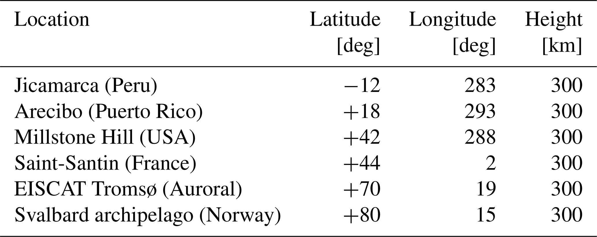
The IRI data are subsequently used in a manner analogous to that in the SAMI2 model of the Naval Research Laboratory (https://github.com/NRL-Plasma-Physics-Division/SAMI2, last access: 1 June 2025). In the present implementation, the ionospheric equations follow the SAMI2 framework originally developed by Huba et al. (2000) and described in detail by Huba (2023). In SAMI2, the neutral atmospheric parameters – namely the neutral number density, total mass density, and temperature – are specified using the MSIS family of models. In this study, these parameters are based on the MSIS formulation of Hedin (1987), while we note that more recent updates are provided by the NRLMSIS 2.0 model of Emmert et al. (2021). The meridional and zonal winds are specified using the Horizontal Wind Model. In the present implementation, we follow the formulation of Hedin et al. (1991), while more recent updates are described by Drob et al. (2015).

The derivatives of the background parameters are computed using central finite differences. Prior to the finite-difference calculations, the background parameters are smoothed using cubic smoothing splines with a regularization (roughness-penalty) term to suppress small-scale numerical fluctuations (Reinsch, 1967; Wahba, 1990).

Other features of the model are summarized as follows:

1. Two linearization models are included in the code:

   • a.

     a general model that accounts for the altitude derivatives of the background velocity, temperature, density scale height, and dynamic viscosity; and

   • b.

     a simplified model for a windless atmosphere without ion drag, in which the gradients of the background temperature and kinematic viscosity are neglected.

2. The methods for solving the linearized equations based on the matrix exponential formalism comprise:

   • a.

     the Global Matrix Method for the Amplitudes (GMMA) of the characteristic solutions, described in Sect. 3.1;

   • b.

     the Scattering Matrix Method for the Amplitudes (SMMA) of the characteristic solutions, described in Sect. 3.2; and

   • c.

     the Global Matrix Method for the Nodal (grid-point) values (GMMN) of the state vector, described in Appendix C.

3. At the lower boundary, we impose that a selected component of the state vector is finite and that its first and second derivatives with respect to height vanish. At the upper boundary, we assume that there is no downward energy propagation, i.e., the amplitudes of all descending wave modes are set to zero.

4. The code first computes the wave parameters for a single-frequency wave and then for a time-dependent wave packet.

5. Typical values of the horizontal wavelength lie in the range 300–700 km.

6. For a single-frequency wave, the output quantity of interest is $\mathcal{A}{\stackrel{\mathrm{‾}}{f}}_{\mathrm{s}q}\left(z\right)$, where ${\stackrel{\mathrm{‾}}{f}}_{\mathrm{s}q}\left(z\right)$ and 𝒜 are given by Eqs. (101) and (103), respectively, whereas for a time-dependent wave packet the corresponding output quantity is $\mathcal{A}{\stackrel{\mathrm{‾}}{f}}_{\mathit{\delta }q}(z,t)$, where ${\stackrel{\mathrm{‾}}{f}}_{\mathit{\delta }q}(z,t)$ and 𝒜 are given by Eqs. (115) and (116), respectively.

6 Numerical simulations

The simulations are performed using, as input, an IRI data file corresponding to the EISCAT Tromsø (auroral) location on 11 February 2012 at 10:00 UT. The solar zenith angle is 84.2°, the magnetic inclination angle is 78.28°, the daily solar radio flux F10.7 is 109.4 sfu, and the 81 d averaged solar radio flux is 116.9 sfu, where $\mathrm{1}\text{sfu}={\mathrm{10}}^{-\mathrm{22}}$ W m⁻² Hz⁻¹. The geomagnetic activity parameter Ap is set to 7.0, corresponding to slightly disturbed geomagnetic conditions. In the simulations, the Prandtl number is 0.66, and the horizontal wind model 14 implemented in SAMI2 is used. The altitude grid extends from 80 to 500 km and contains 801 grid points. The lower boundary can, in principle, be set to smaller altitudes (e.g., 50 km), but we choose 80 km because this level is typically adopted as the lower boundary for ionospheric equations. Unless stated otherwise, the horizontal wavelength is λ_x=400 km, the wave period is λ_t=40 min, and the imaginary frequency shift for a single-frequency wave is 10⁻⁶ s⁻¹. The lower boundary conditions are imposed on the vertical velocity with $f_{\text{b2}}=\mathrm{5}\times {\mathrm{10}}^{-\mathrm{2}}$ ms⁻¹ in Eqs. (86) and (102).

6.1 Accuracy and efficiency of the solution methods

Taking the global matrix method for amplitudes as a reference, we find that the relative root-mean-square errors in the perturbed temperature, vertical velocity, and horizontal velocity obtained with the other two solution methods are smaller than 10⁻⁶. Thus, all methods exhibit comparable accuracy. On the other hand, we find that the scattering matrix method is more time-consuming than the global matrix methods, particularly for time-dependent wave packets. This is because the scattering matrix approach requires numerous matrix operations in each layer, whereas solving a system of equations compressed into band storage is computationally less expensive.

6.2 Background atmospheric parameters

The numerical model uses altitude-dependent profiles of atmospheric and ionospheric parameters, including temperature, mass density, pressure, southward horizontal velocity, atmospheric scale height, density scale height, specific heat capacity, ratio of specific heats, sound speed, O⁺ ion number density, neutral–ion collision frequency, ion–neutral collision frequency, and the background field-aligned ambipolar diffusion velocity (see Appendix B). In addition, the altitude derivatives of temperature, horizontal velocity, mass density, pressure, density scale height, and ion number density are required. Figure 1 shows the background temperature T₀, horizontal velocity u₀ and the ion number density n_i0, together with their corresponding altitude derivatives.

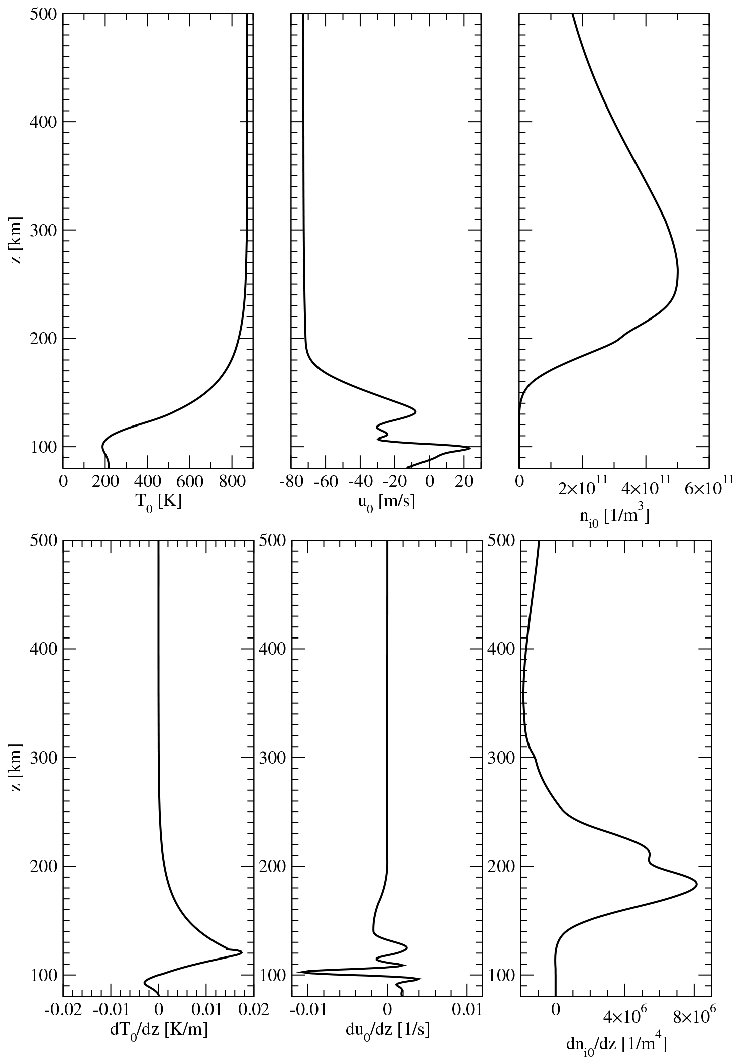
Figure 1 Background temperature T₀, horizontal velocity u₀ and ion number density n_i0 ($i={\text{O}}^{+}$) (upper panels), and their height derivatives (lower panels).

6.3 Pairwise classification of ascending and descending modes

Figure 2 compares the imaginary parts of the vertical wavenumbers associated with the ascending and descending gravity-wave modes. The upper panel shows the results obtained with the general model, including ion drag, while the second panel shows the corresponding results for the simplified model. In the general model, the imaginary parts of the ascending and descending vertical wavenumbers approach each other in the altitude range from approximately 80 to 170 km. To illustrate the degree of separation between these two modes, the third and fourth panels show the quantity Im(k_z4)−Im(k_z1) on a logarithmic scale for the general and simplified models, respectively. These plots demonstrate that the imaginary parts of the two gravity-wave modes remain separated at all altitudes, although the separation becomes very small in the transition region. A complete assessment of branch continuity, however, requires consideration of both the real and imaginary parts of the vertical wavenumbers. Additional numerical experiments indicate that the real parts of the ascending and descending gravity-wave modes cross near the altitudes (approximately 105 and 175 km) where sharp changes in the quantity Im(k_z4)−Im(k_z1) are observed. A detailed investigation of the root-tracking procedure and the influence of the imaginary frequency shift on branch continuity will be the subject of future research. Figure 3 shows the imaginary parts of the vertical wavenumbers for all wave modes $(k_{zn},n=\mathrm{1},\mathrm{\dots },\mathrm{6})$ computed using the general model. The plot illustrates the clear separation between the gravity-wave modes and the viscosity- and thermal-conduction modes. The latter two mode pairs approach each other most closely in the altitude range around 100 km.

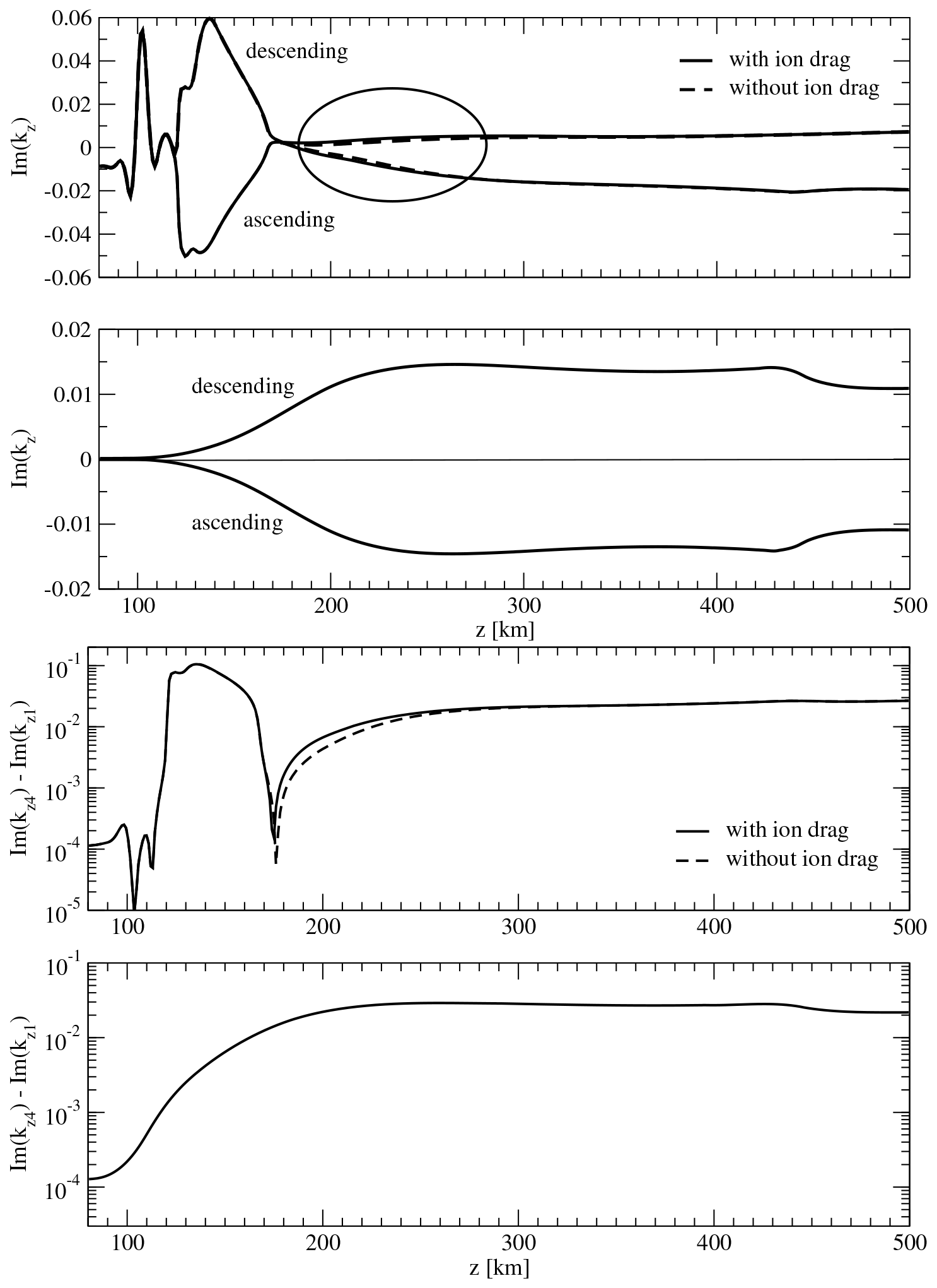
Figure 2 Comparison of the imaginary parts of the vertical wavenumbers associated with the ascending (k_z1) and descending (k_z4) gravity-wave modes. Upper panel: Im(k_z) computed using the general model, with and without ion drag. The oval indicates the altitude region where ion drag produces a small deviation in the vertical wavenumbers. Second panel: Im(k_z) for the ascending and descending gravity-wave modes computed using the simplified model. Third panel: logarithmic plot of Im(k_z4)−Im(k_z1) for the general model. Fourth panel: logarithmic plot of Im(k_z4)−Im(k_z1) for the simplified model. The results correspond to λ_x=400 km and λ_t=40 min.

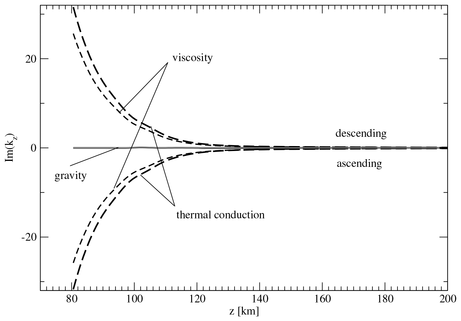
Figure 3 Imaginary parts of the vertical wavenumbers for all wave modes $(k_{zn},n=\mathrm{1},\mathrm{\dots },\mathrm{6})$ computed using the general model. The figure shows the gravity-wave modes together with the viscosity and thermal-conduction modes. The results correspond to λ_x=400 km and λ_t=40 min.

6.4 General and simplified models

The altitude profiles of the perturbed temperature, vertical velocity, and horizontal velocity computed using the general and simplified models are shown in Fig. 4. The plots show that, in the altitude range 150–300 km, the amplitudes obtained with the general model are larger than those obtained with the simplified model. If the imaginary parts of the vertical wavenumber for ascending gravity waves computed with the general and simplified models were plotted on the same graph (i.e. by merging the lower and middle panels of Fig. 2), it would be seen that the imaginary part of the vertical wavenumber corresponding to the general model is negative but larger (i.e., less negative) than that obtained with the simplified model. As a consequence, the exponential attenuation with altitude is weaker in the general model, leading to systematically larger wave amplitudes in this region. This behavior reflects the modified balance between wave propagation and dissipation introduced by the inclusion of altitude-dependent background properties and by relaxing the assumption of constant kinematic viscosity, which reduces the effective vertical damping relative to the simplified model. In addition to the amplitude differences, Fig. 4 exhibits substantial phase shifts between the solutions of the general and simplified models. These phase shifts can be attributed to differences in the imaginary part of the eigenvalue, or equivalently, in the real part of the vertical wavenumber of the ascending gravity-wave mode. Since the wave phase accumulates with altitude in proportion to the real part of the vertical wavenumber, even moderate differences between the gravity-wave roots of the two models lead to noticeable displacements of the extrema of the temperature and velocity perturbations.

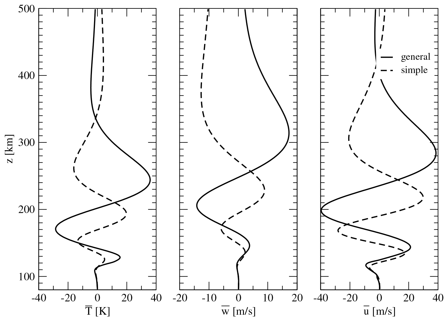
Figure 4 Altitude profiles of the perturbed temperature $\stackrel{\mathrm{‾}}{T}$, vertical velocity $\stackrel{\mathrm{‾}}{w}$, and horizontal velocity $\stackrel{\mathrm{‾}}{u}$ for the general and simplified models. The results correspond to λ_x=400 km and λ_t=40 min.

6.5 Ion Drag

The effect of ion drag on the perturbed temperature, vertical velocity, and horizontal velocity is illustrated in Fig. 5. A moderate attenuation is observed in the altitude range from 180 to 350 km, where the ion number density is relatively high. In the present model, E×B drift velocities are neglected, and the ion velocity is approximated by the field-aligned neutral velocity plus the field-aligned ambipolar diffusion velocity (see Appendix B). Consequently, the classical auroral-convection regime, in which E×B-driven ion motion transfers momentum and energy to the neutral atmosphere through ion drag, is not represented here (Richmond and Matsushita, 1975; Fuller-Rowell and Rees, 1984). Instead, ion drag arises primarily from field-aligned ambipolar diffusion and from relative ion–neutral motion induced by neutral winds. As a result, ion drag acts mainly as a secondary damping mechanism and does not constitute the dominant forcing of the neutral perturbations in the present simulations.

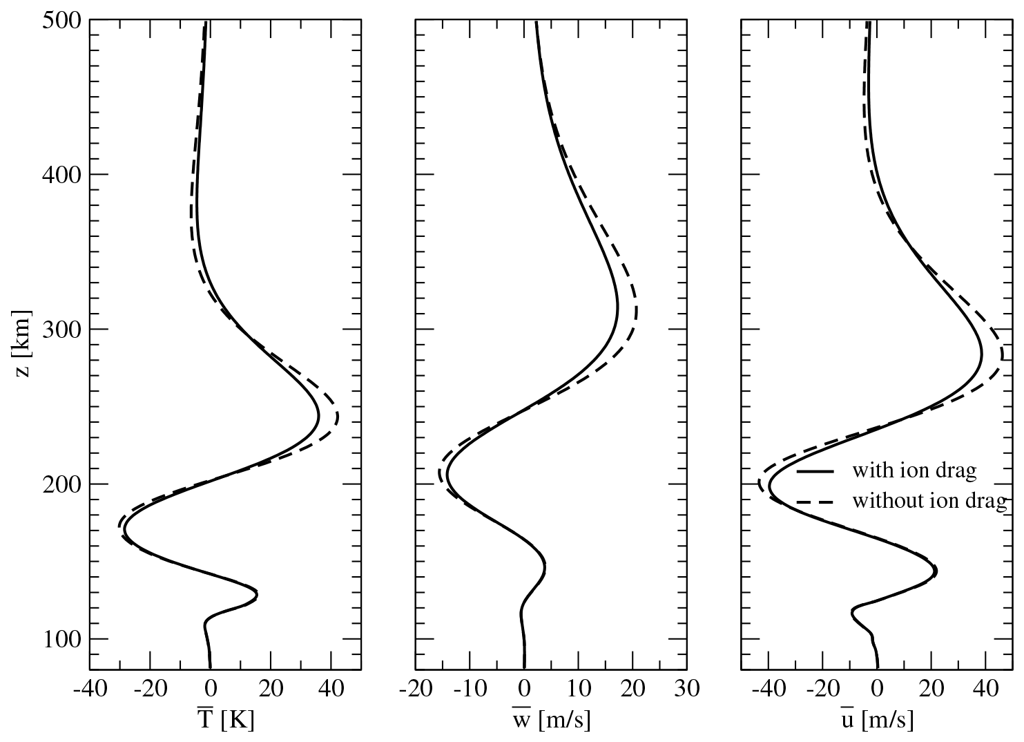
Figure 5 Altitude profiles of the perturbed temperature $\stackrel{\mathrm{‾}}{T}$, vertical velocity $\stackrel{\mathrm{‾}}{w}$, and horizontal velocity $\stackrel{\mathrm{‾}}{u}$ for the general model, with and without ion drag. The results correspond to λ_x=400 km and λ_t=40 min.

6.6 Horizontal wavelength and time period

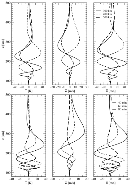
The influence of the horizontal wavelength λ_x and the wave period λ_t on the perturbed quantities is shown in Fig. 6. The results indicate that, for the same lower-boundary amplitude, waves with larger horizontal wavelengths and longer periods generally attain smaller amplitudes at higher altitudes. In the inviscid region, the altitude variation of the wave amplitude is controlled primarily by the density stratification through the $\mathrm{j}/\left(\mathrm{2}{H}_{\text{a}}\right)$ contribution to the vertical wavenumber (cf. Eq. 18) and is therefore largely independent of the horizontal wavelength and wave period. At higher altitudes, however, viscosity and thermal conduction become increasingly important, and the attenuation rate is determined by the imaginary part of the vertical wavenumber of the ascending gravity-wave mode. Since the horizontal wavelength and wave period modify the gravity-wave dispersion relation, they also modify the corresponding vertical wavenumber and its attenuation rate. Consequently, waves with different values of λ_x and λ_t experience different amounts of dissipation during upward propagation, leading to the amplitude differences observed in Fig. 6. The dependence on λ_x and λ_t can therefore be understood in terms of the corresponding gravity-wave roots computed by the model, whose imaginary parts determine the attenuation rates and whose real parts determine the phase propagation characteristics. Because the plotted quantities are signed perturbations, differences in the real part of the vertical wavenumber may also produce noticeable phase shifts between the profiles. Consequently, the 400 km profiles do not necessarily lie between the 300 and 500 km profiles, even though all solutions are normalized to the same prescribed lower-boundary amplitude $f_{\text{b}{q}_{\mathrm{0}}}$ of the selected perturbation component.

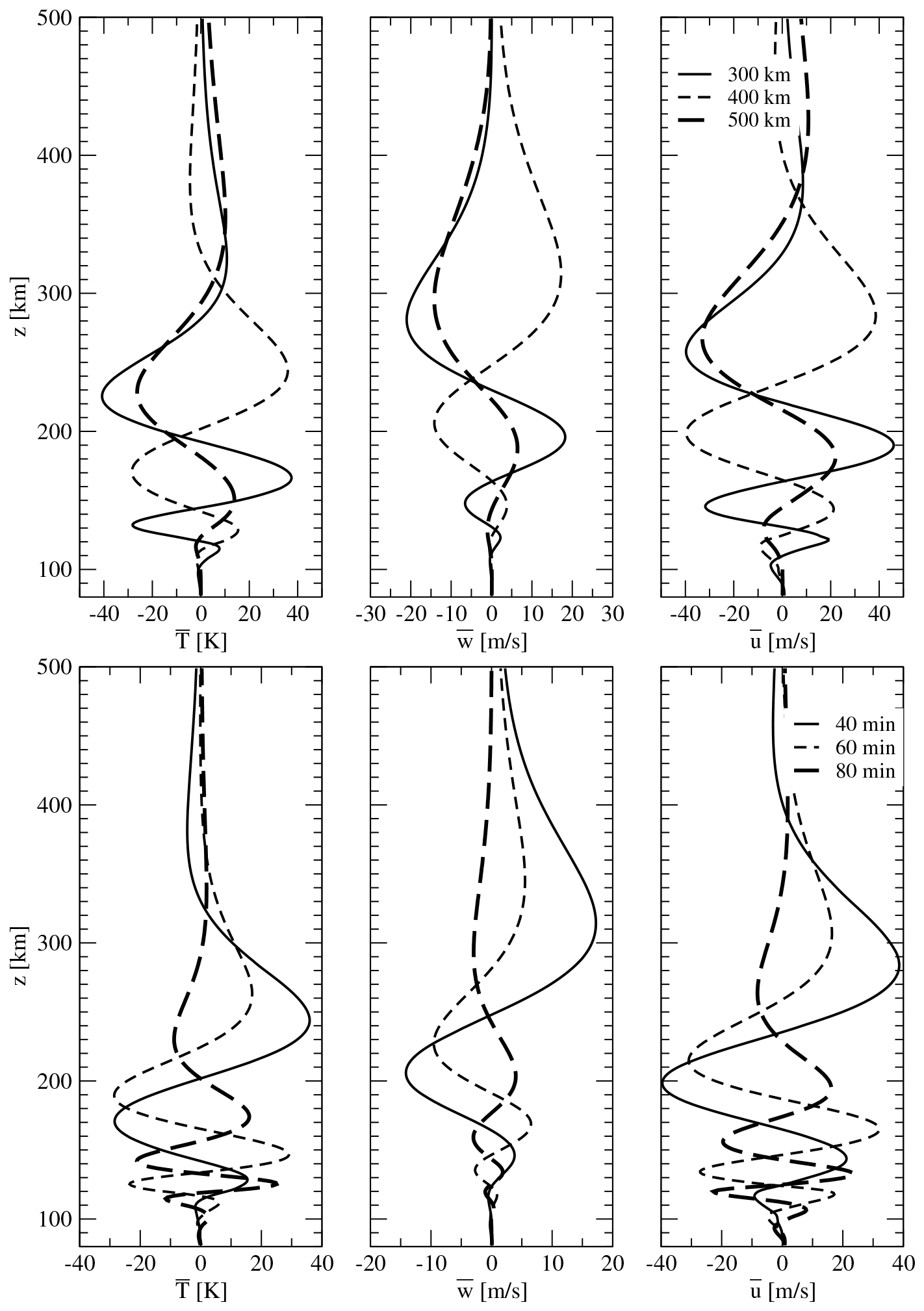
Figure 6 Altitude profiles of the perturbed temperature $\stackrel{\mathrm{‾}}{T}$, vertical velocity $\stackrel{\mathrm{‾}}{w}$, and horizontal velocity $\stackrel{\mathrm{‾}}{u}$ for (i) λ_x=300, 400, and 500 km with λ_t=40 min (upper panels), and (ii) λ_x=400 km with λ_t=40, 60, and 80 min (lower panels). The results correspond to the general model with ion drag.

6.7 Computing ascending and descending wave solutions

The ascending and descending wave contributions in layer l, denoted by ${\mathit{e}}_l^{+}$ and ${\mathit{e}}_l^{-}$, respectively, can be computed using the GMMA through Eq. (62) or using the GMMN via the recurrence relations (C11) and (C12). The total solution e_l, obtained from Eq. (60) in the GMMA formulation and by solving Eq. (C8) in the GMMN formulation, should satisfy the relation ${\mathit{e}}_l={\mathit{e}}_l^{+}+{\mathit{e}}_l^{-}.$ This identity was verified in all computations and was used as an internal consistency check of the code. Furthermore, the results shown in Fig. 7 indicate that the ascending-wave contribution is dominant, except in the altitude range between 120 km and 180 km in the case of the general model. This finding, which is consistent with the results presented by Knight et al. (2019) (see their Fig. 6), suggests that in a simplified model one may assume the ascending-wave contribution to be dominant at altitudes above 200 km, that is, ${\mathit{e}}_l\approx {\mathit{e}}_l^{+}$ for $l=\mathrm{1},\mathrm{\dots },L$. Under this assumption, the state vector can be computed using the upward recurrence relation (C11). In Knight et al. (2019), this approach was referred to as the transmission-only approximation, whereas in Knight et al. (2021) a related single-mode approximation was introduced.

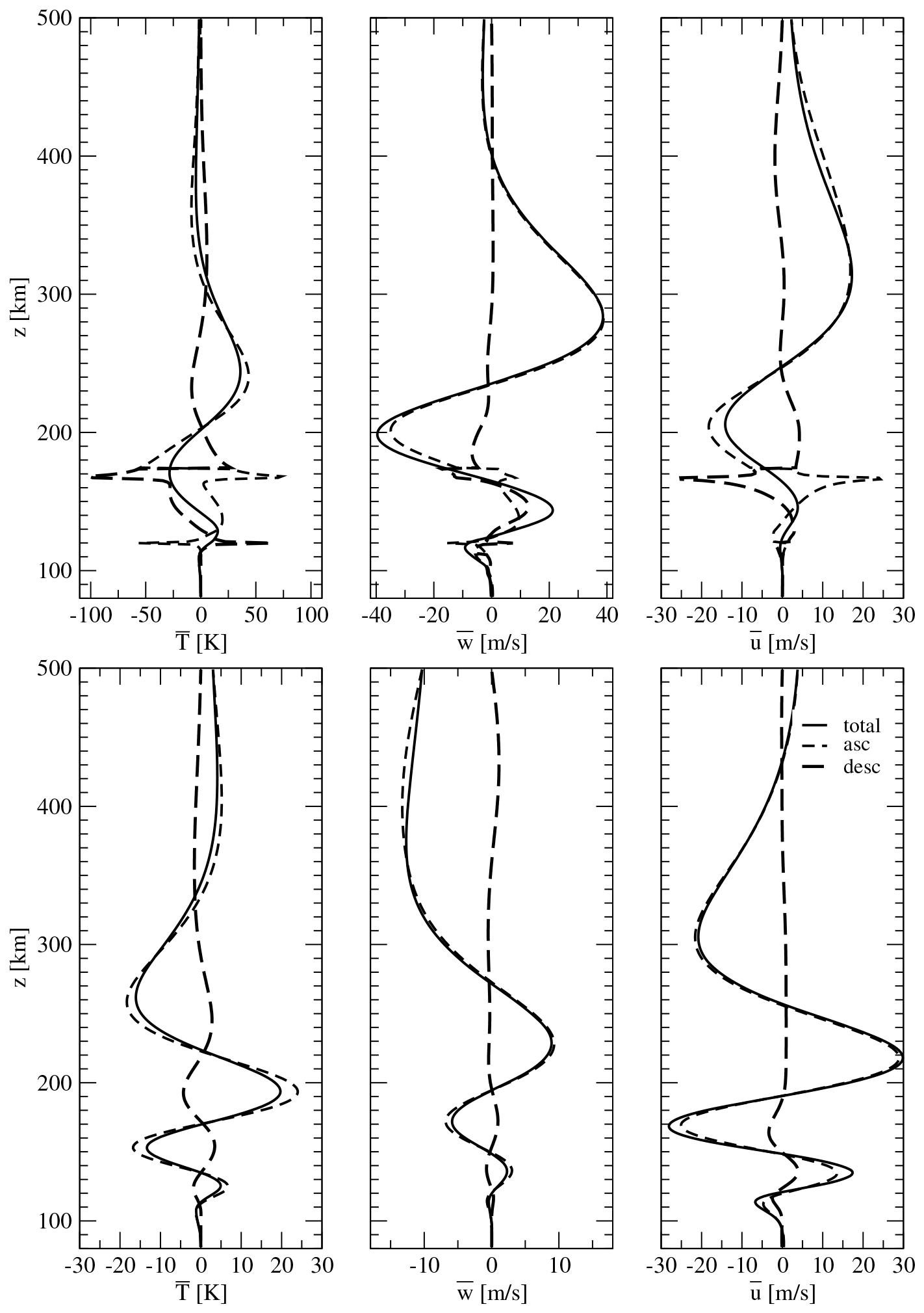
Figure 7 Altitude profiles of the perturbed temperature $\stackrel{\mathrm{‾}}{T}$, vertical velocity $\stackrel{\mathrm{‾}}{w}$, and horizontal velocity $\stackrel{\mathrm{‾}}{u}$ for the total solution (${\mathit{e}}_l={\mathit{e}}_l^{+}+{\mathit{e}}_l^{-}$ in layer l), the ascending-wave solution (${\mathit{e}}_l^{+}$), and the descending-wave solution (${\mathit{e}}_l^{-}$). The upper panels correspond to the general model, and the lower panels to the simplified model. The horizontal wavelength is λ_x=400 km and the wave period is λ_t=40 min.

6.8 Time-dependent wave packet

For the source function (83)–(84), Fig. 8 shows the perturbed temperature and vertical velocity as functions of time and altitude. Note the different time intervals used for each horizontal wavelength λ_x in these plots. The maximum values of the perturbed temperature are 32.21, 31.15, and 32.73 K for the horizontal wavelengths 300, 500, and 700 km, respectively, whereas the corresponding maximum values of the vertical velocity are 21.40, 16.21, and 12.08 m s⁻¹. The practical implementation of the wave-packet calculations, including the choice of the frequency and time discretizations used for the Fourier-transform evaluation, is described in Appendix D.

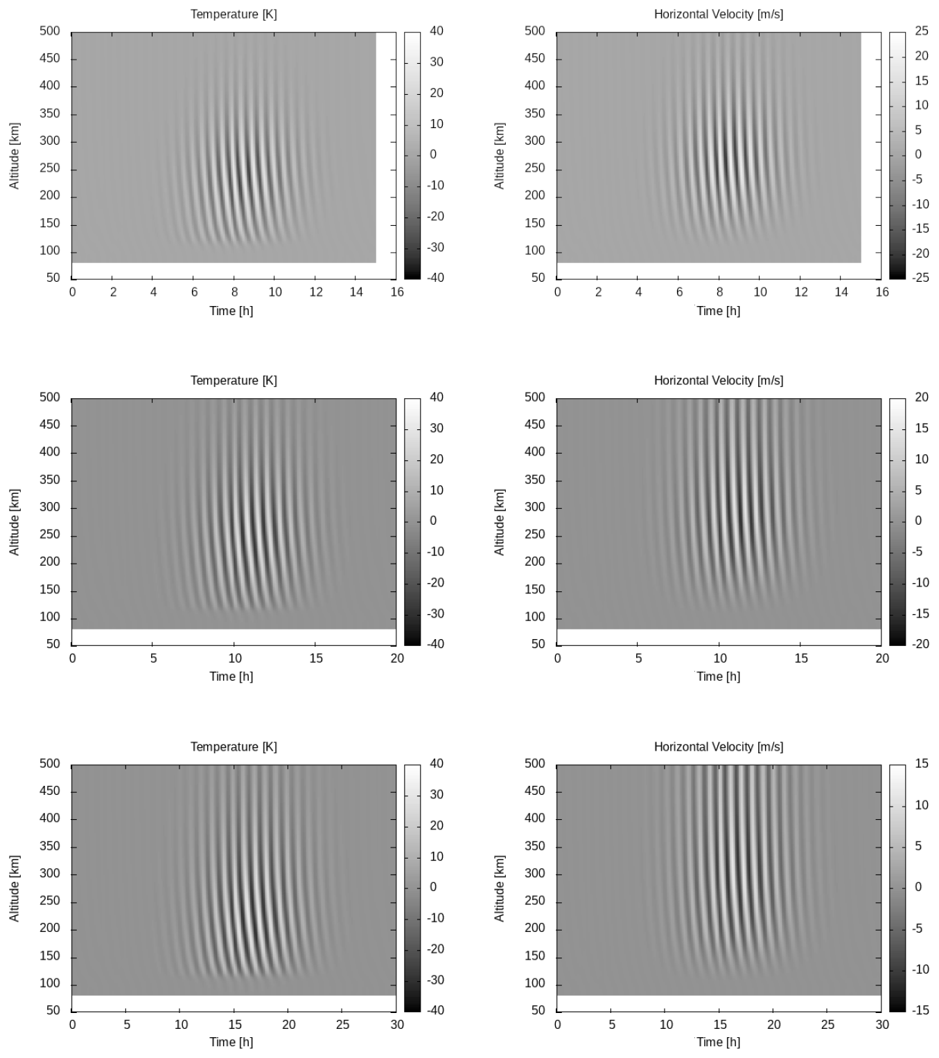
Figure 8 Perturbed temperature (left panels) and vertical velocity (right panels) as functions of time and altitude. The upper panels correspond to λ_x=300 km and λ_t=30 min, the middle panels to λ_x=500 km and λ_t=40 min, and the lower panels to λ_x=700 km and λ_t=60 min.

6.9 Imaginary frequency shift

The determination of the admissible interval of imaginary frequency shifts follows the procedure described in Appendix D. For the present case λ_x=500 km and λ_t=40 min, this procedure yields the interval $[{\mathit{\delta }}_{min}={\mathrm{10}}^{-\mathrm{6}}$ s${}^{-\mathrm{1}},{\mathit{\delta }}_{max}=\mathrm{32.24}\times {\mathrm{10}}^{-\mathrm{6}}$ s⁻¹], within which the search for admissible solutions is performed. Specifically, candidate solutions corresponding to values of δ in this interval are examined, and only those satisfying the layerwise causality condition throughout the entire altitude range are retained. Five equidistant values of the imaginary frequency shift δ within this interval were considered. For each value, the wave parameters were computed and the layerwise causality condition was verified throughout the entire altitude range. All five solutions satisfied this condition and produced nearly identical maximum values of the perturbed horizontal velocity, vertical velocity, and temperature (Table 2). This behavior is expected because, once the layerwise causality condition is satisfied, the physical solution is not expected to depend on the particular value of the imaginary frequency shift δ, provided that δ remains within the admissible interval (see Knight et al., 2022, following Eq. 2.58). To select a representative solution, we considered the three-dimensional space formed by the maximum amplitudes (${\stackrel{\mathrm{‾}}{u}}_{max},{\stackrel{\mathrm{‾}}{w}}_{max},{\stackrel{\mathrm{‾}}{T}}_{max}$). The final solution was chosen as the one whose amplitude vector is closest to the center of mass of the five candidate solutions. This criterion yields the third solution, corresponding to $\mathit{\delta }=\mathrm{16.62}\times {\mathrm{10}}^{-\mathrm{6}}$ s⁻¹. For this solution, the maxima occur at 11.06 h and 248.00 km for the horizontal velocity, 10.98 h and 303.64 km for the vertical velocity, and 10.90 h and 257.45 km for the temperature. To assess the sensitivity of the solution to the choice of δ, Fig. 9 shows the relative Root-Mean-Square (RMS) differences in the perturbed horizontal velocity, vertical velocity, and temperature between the selected solution and the remaining solutions. For each altitude, the relative RMS difference is computed over the entire time interval by dividing the RMS difference by the RMS value of the corresponding field of the selected solution over the same time interval.

Table 2 Maximum values of the perturbed horizontal velocity (${\stackrel{\mathrm{‾}}{u}}_{max}$), vertical velocity (${\stackrel{\mathrm{‾}}{w}}_{max}$), and temperature (${\stackrel{\mathrm{‾}}{T}}_{max}$) for different values of the imaginary frequency shift δ. The selected solution is the third solution corresponding to $\mathit{\delta }=\mathrm{16.62}\times {\mathrm{10}}^{-\mathrm{6}}$ s⁻¹.

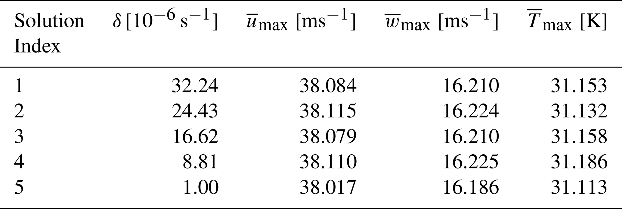
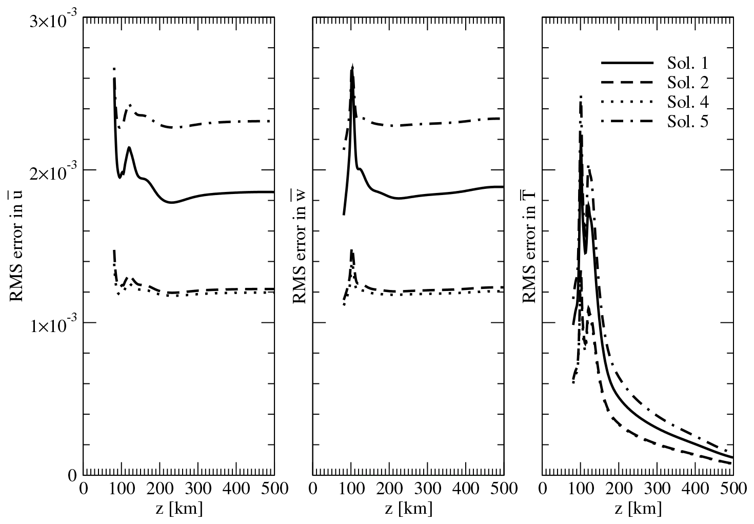
Figure 9 Relative Root-Mean-Square (RMS) differences in the perturbed horizontal velocity $\stackrel{\mathrm{‾}}{u}$, vertical velocity $\stackrel{\mathrm{‾}}{w}$, and temperature perturbation $\stackrel{\mathrm{‾}}{T}$ between the selected solution ($\mathit{\delta }=\mathrm{16.62}\times {\mathrm{10}}^{-\mathrm{6}}$ s⁻¹) and the remaining solutions corresponding to different values of the imaginary frequency shift δ. For each altitude, the relative RMS difference is computed over the entire simulation time interval by dividing the RMS difference by the RMS value of the corresponding field of the selected solution over the same time interval.

7 Conclusions

We designed a numerical model for solving the linearized gravity-wave equations using a multilayer method, which is freely available as open-source code at https://github.com/AlexandruDoicu/Gravity-Waves (last access: 1 June 2026) . To decouple the hydrodynamic equations for the neutral atmosphere from the ionospheric equations, which are coupled through ion drag, we adopt a fast field-aligned diffusion approximation. This approximation may be viewed as a generalization of an approach originally proposed by Klostermeyer (1972).

To solve the linearized equations, we employ (i) global matrix methods based on matrix exponentials and (ii) scattering matrix methods to determine either (a) the amplitudes of the characteristic solutions or (b) the grid-point values of the state vector. Ascending and descending wave modes are identified according to the criterion that the real parts of the eigenvalues of the characteristic equation for ascending modes are smaller than those for descending modes (or, equivalently, that the imaginary parts of the vertical wavenumbers are smaller). Global matrix methods using the scaling matrices (36) and (37) require the classification of ascending and descending modes only at the lower and upper boundaries, whereas scattering matrix methods require an explicit determination of the mode type at every altitude. The model is devoted to solving the linearized equations including viscosity, thermal conduction, and ion drag. A simplified model for a windless atmosphere without ion drag is also considered, in which the altitude derivatives of the background temperature and kinematic viscosity are neglected.

Depending on the form of the source function, either single-frequency waves or time-dependent wave packets can be analyzed. A heuristic approach for determining the imaginary frequency shift introduced by Knight et al. (2019) is also considered. This approach is based on (i) a layerwise causality condition applied at selected altitude levels, and (ii) a source-function reconstruction test.

Numerical simulations demonstrate that both global matrix and scattering matrix methods achieve comparable accuracy. However, the former are significantly more efficient than the latter, particularly in simulations involving time-dependent wave packets. Among the global matrix methods, the approach based on solving for the amplitudes of the characteristic solutions appears to provide the highest efficiency and accuracy.

The linearized equations on which the solution methods were tested correspond to ionospheric conditions. The ultimate goal of our research is to develop a comprehensive model for analyzing ionospheric gravity waves using satellite measurements. The approach presented in this paper represents only the first component of such a model. Two options are envisaged for extending it to a more complete formulation.

1. Fully coupled neutral–ion model. The linearized hydrodynamic equations would be solved together with the ion equations. In this case, the ion continuity equation would include perturbed production and loss terms, whereas ion inertia and ion–ion collisions would continue to be neglected in the ion momentum equation, and only transport parallel to the magnetic field lines would be retained. The state vector would then be augmented by two additional components, namely the perturbed ion number density and the ion diffusion velocity.

2. Two-step coupling strategy. In the first step, the neutral-atmosphere equations are solved using the fast field-aligned diffusion approximation. In the second step, the wave-induced perturbations obtained from the neutral solution are used as input to solve the ionospheric equations for the perturbed O⁺ ion density. The ionospheric equations may be solved using the SAMI2 model (Huba et al., 2000) for low latitudes, where the E×B drift is neglected, or the SAMI3 model (Huba et al., 2008) at higher altitudes, where the E×B drift is included and the electric field is determined from the solution of a two-dimensional potential equation. In this strategy, priority is given to the ionospheric equations of the SAMI framework, while wave-induced perturbations are handled using the approximate approach developed in the present study. Along similar lines, Knight et al. (2025) solved the neutral-atmosphere equations without ion drag in a first step, and subsequently addressed the ionospheric response using the Field-Line Interhemispheric Plasma (FLIP) model (Richards and Peterson, 2008).

The development and application of these complete models will be addressed in future papers.

Appendix A: Derivation of the linear system of ordinary differential equations

In this appendix, we derive the explicit representation of the linear system of ordinary differential equations (5).

A1 Hydrodynamic equations

The hydrodynamic equations for the neutral atmosphere consist in the continuity, momentum, heat, and ideal gas equations (e.g., Midgley and Liemohn, 1966; Volland, 1969b)

$$\begin{array}{}\text{(A1)}& {\displaystyle \frac{\mathrm{D}\mathit{\rho }}{\mathrm{D}t}}& {\displaystyle }=-\mathit{\rho }\mathrm{\nabla }\cdot \mathit{u},\text{(A2)}& {\displaystyle }\mathit{\rho }{\displaystyle \frac{\mathrm{D}\mathit{u}}{\mathrm{D}t}}& {\displaystyle }=-\mathrm{\nabla }p+\mathit{\rho }\mathit{g}+\mathrm{\nabla }\cdot \stackrel{\mathrm{‾}}{\mathit{\sigma }}-{\mathit{f}}_{\text{ID}},\text{(A3)}& {\displaystyle }\mathit{\rho }{c}_{\text{v}}{\displaystyle \frac{\mathrm{D}T}{\mathrm{D}t}}& {\displaystyle }=-p\mathrm{\nabla }\cdot \mathit{u}+\stackrel{\mathrm{‾}}{\mathit{\sigma }}:\mathrm{\nabla }\mathit{u}+\mathrm{\nabla }\cdot \left(\mathrm{\Lambda }\mathrm{\nabla }T\right)-q_{\text{ID}},\text{(A4)}& {\displaystyle }p& {\displaystyle }=\mathit{\rho }{R}_{M}T,\end{array}$$

where ρ is the density, p the pressure, T the temperature, u the velocity, g the gravitational acceleration vector, $\mathrm{D}/\mathrm{D}t=\partial /\partial t+\mathit{u}\cdot \mathrm{\nabla }$ the material (substantial) derivative, c_v the specific heat at constant volume, Λ the coefficient of thermal conductivity, R_M the specific gas constant, and $\stackrel{\mathrm{‾}}{\mathit{\sigma }}$ the viscous stress tensor. The quantities f_ID and q_ID denote the ion-drag force exerted by neutrals on ions per unit volume, and the frictional heating rate per unit volume arising from ion–neutral collisions, respectively. In a Cartesian coordinate system $(x_{\mathrm{1}},x_{\mathrm{2}},x_{\mathrm{3}})$, the components of the viscous stress tensor are given by

$$\begin{array}{}\text{(A5)}& {\mathit{\sigma }}_{ij}=\mathit{\mu }\left({\displaystyle \frac{\partial u_i}{\partial x_{\mathrm{j}}}}+{\displaystyle \frac{\partial u_{\mathrm{j}}}{\partial x_i}}-{\displaystyle \frac{\mathrm{2}}{\mathrm{3}}}{\mathit{\delta }}_{ij}\mathrm{\nabla }\cdot \mathit{u}\right),\end{array}$$

where μ is the dynamic viscosity and δ_ij the Kroneker delta. Accordingly, the double dot product of $\stackrel{\mathrm{‾}}{\mathit{\sigma }}={\sum }_{ij}{\mathit{\sigma }}_{ij}{\widehat{\mathit{x}}}_i\otimes {\widehat{\mathit{x}}}_{\mathrm{j}}$ with $\mathrm{\nabla }\mathit{u}={\sum }_{ij}\partial u_i/\partial x_{\mathrm{j}}{\widehat{\mathit{x}}}_i\otimes {\widehat{\mathit{x}}}_{\mathrm{j}}$ is

$$\begin{array}{}\text{(A6)}& \stackrel{\mathrm{‾}}{\mathit{\sigma }}:\mathrm{\nabla }\mathit{u}=\sum _{ij}{\mathit{\sigma }}_{ij}{\displaystyle \frac{\partial u_i}{\partial x_{\mathrm{j}}}}.\end{array}$$

Using the ideal-gas law p=ρR_MT so that $\mathrm{\nabla }p=\mathit{\rho }{R}_M\mathrm{\nabla }T+R_{M}T\mathrm{\nabla }\mathit{\rho }$, the momentum equation can be written as

$$\begin{array}{}\text{(A7)}& \begin{array}{rl}{\displaystyle \frac{\partial \mathit{u}}{\partial t}}& =-{\displaystyle \frac{R_{M}T}{\mathit{\rho }}}\mathrm{\nabla }\mathit{\rho }-R_M\mathrm{\nabla }T-(\mathit{u}\cdot \mathrm{\nabla })\mathit{u}\\ & +\mathit{g}+{\displaystyle \frac{\mathrm{1}}{\mathit{\rho }}}\mathrm{\nabla }\cdot \stackrel{\mathrm{‾}}{\mathit{\sigma }}-{\displaystyle \frac{\mathrm{1}}{\mathit{\rho }}}{\mathit{f}}_{\text{ID}}.\end{array}\end{array}$$

Moreover, using

$$\begin{array}{}\text{(A8)}& c_p=c_{\text{v}}+R_M,\mathit{\gamma }={\displaystyle \frac{c_p}{c_{\text{v}}}},\mathrm{\Lambda }={\displaystyle \frac{c_p\mathit{\mu }}{Pr}},\end{array}$$

where c_p is the specific heat at constant pressure, γ the ratio of specific heats, and Pr the Prandtl number, and assuming that c_p and Pr are constant, the heat equation becomes

$$\begin{array}{}\text{(A9)}& \begin{array}{rl}{\displaystyle \frac{\partial T}{\partial t}}& =-\left(\mathit{\gamma }-\mathrm{1}\right)T\mathrm{\nabla }\cdot \mathit{u}-\mathit{u}\cdot \mathrm{\nabla }T\\ & +{\displaystyle \frac{\mathrm{1}}{\mathit{\rho }{c}_{\text{v}}}}\stackrel{\mathrm{‾}}{\mathit{\sigma }}:\mathrm{\nabla }\mathit{u}+{\displaystyle \frac{\mathit{\gamma }}{\mathit{\rho }Pr}}\mathrm{\nabla }\cdot \left(\mathit{\mu }\mathrm{\nabla }T\right)-{\displaystyle \frac{\mathrm{1}}{\mathit{\rho }{c}_{\text{v}}}}{q}_{\text{ID}}.\end{array}\end{array}$$

In the momentum and heat equations, the ion-drag force and the corresponding heating per unit mass are given by

$$\begin{array}{}\text{(A10)}& {\displaystyle \frac{\mathrm{1}}{\mathit{\rho }}}{\mathit{f}}_{\text{ID}}& {\displaystyle }={\mathit{\nu }}_{ni}(\mathit{u}-{\mathit{u}}_i),\text{(A11)}& {\displaystyle \frac{\mathrm{1}}{\mathit{\rho }}}{q}_{\text{ID}}& {\displaystyle }={\displaystyle \frac{\mathrm{1}}{\mathit{\rho }}}{\mathit{f}}_{\text{ID}}\cdot (\mathit{u}-{\mathit{u}}_i)={\mathit{\nu }}_{ni}|\mathit{u}-{\mathit{u}}_i{|}^{\mathrm{2}},\end{array}$$

where ν_ni is the neutral-ion collision frequency (the collision frequency between a neutral particle and all kind of ions).

We choose a rectangular coordinate system such that the x-axis is directed to the geographic south, the y-axis to the east and the z-axis upward. The wave propagates in the meridional plane, i.e., in the (x,z) plane. The viscous terms per unit mass in the momentum equation are then given by

$$\begin{array}{ll}{\displaystyle \frac{\mathrm{1}}{\mathit{\rho }}}(\mathrm{\nabla }\cdot \stackrel{\mathrm{‾}}{\mathit{\sigma }}{)}_x& {\displaystyle }={\mathit{\mu }}_{\text{k}}\left[\left({\displaystyle \frac{{\partial }^{\mathrm{2}}u}{\partial x^{\mathrm{2}}}}+{\displaystyle \frac{{\partial }^{\mathrm{2}}u}{\partial z^{\mathrm{2}}}}\right)+{\displaystyle \frac{\mathrm{1}}{\mathrm{3}}}\left({\displaystyle \frac{{\partial }^{\mathrm{2}}u}{\partial x^{\mathrm{2}}}}+{\displaystyle \frac{{\partial }^{\mathrm{2}}w}{\partial x\partial z}}\right)\right]\\ \text{(A12)}& {\displaystyle }& {\displaystyle }+{\displaystyle \frac{\mathrm{1}}{\mathit{\rho }}}{\displaystyle \frac{\partial \mathit{\mu }}{\partial z}}\left({\displaystyle \frac{\partial u}{\partial z}}+{\displaystyle \frac{\partial w}{\partial x}}\right),{\displaystyle \frac{\mathrm{1}}{\mathit{\rho }}}(\mathrm{\nabla }\cdot \stackrel{\mathrm{‾}}{\mathit{\sigma }}{)}_z& {\displaystyle }={\mathit{\mu }}_{\text{k}}\left[\left({\displaystyle \frac{{\partial }^{\mathrm{2}}w}{\partial x^{\mathrm{2}}}}+{\displaystyle \frac{{\partial }^{\mathrm{2}}w}{\partial z^{\mathrm{2}}}}\right)+{\displaystyle \frac{\mathrm{1}}{\mathrm{3}}}\left({\displaystyle \frac{{\partial }^{\mathrm{2}}u}{\partial x\partial z}}+{\displaystyle \frac{{\partial }^{\mathrm{2}}w}{\partial z^{\mathrm{2}}}}\right)\right]\\ \text{(A13)}& {\displaystyle }& {\displaystyle }+{\displaystyle \frac{\mathrm{1}}{\mathit{\rho }}}{\displaystyle \frac{\partial \mathit{\mu }}{\partial z}}\left({\displaystyle \frac{\mathrm{4}}{\mathrm{3}}}{\displaystyle \frac{\partial w}{\partial z}}-{\displaystyle \frac{\mathrm{2}}{\mathrm{3}}}{\displaystyle \frac{\partial u}{\partial x}}\right),\end{array}$$

while the viscous dissipation term per unit mass appearing in the heat equation is

$$\begin{array}{ll}{\displaystyle \frac{\mathrm{1}}{\mathit{\rho }}}\stackrel{\mathrm{‾}}{\mathit{\sigma }}:\mathrm{\nabla }\mathit{u}& {\displaystyle }={\displaystyle \frac{\mathrm{4}}{\mathrm{3}}}{\mathit{\mu }}_{\text{k}}{\left({\displaystyle \frac{\partial u}{\partial x}}\right)}^{\mathrm{2}}-{\displaystyle \frac{\mathrm{4}}{\mathrm{3}}}{\mathit{\mu }}_{\text{k}}{\displaystyle \frac{\partial u}{\partial x}}{\displaystyle \frac{\partial w}{\partial z}}+{\displaystyle \frac{\mathrm{4}}{\mathrm{3}}}{\mathit{\mu }}_{\text{k}}{\left({\displaystyle \frac{\partial w}{\partial z}}\right)}^{\mathrm{2}}\\ \text{(A14)}& {\displaystyle }& {\displaystyle }+{\mathit{\mu }}_{\text{k}}{\left({\displaystyle \frac{\partial u}{\partial z}}\right)}^{\mathrm{2}}+\mathrm{2}{\mathit{\mu }}_{\text{k}}{\displaystyle \frac{\partial u}{\partial z}}{\displaystyle \frac{\partial w}{\partial x}}+{\mathit{\mu }}_{\text{k}}{\left({\displaystyle \frac{\partial w}{\partial x}}\right)}^{\mathrm{2}}.\end{array}$$

Here, ${\mathit{\mu }}_{\text{k}}=\mathit{\mu }/\mathit{\rho }$ is the kinematic viscosity, and we have assumed that the viscosity depends only on altitude, so that

$$\begin{array}{}\text{(A15)}& {\displaystyle \frac{\partial \mathit{\mu }}{\partial x}}=\mathrm{0}.\end{array}$$

Using Eqs. (A12)–(A14) together with assumption (A15), we express the momentum and heat equations as

$$\begin{array}{ll}{\displaystyle \frac{\partial u}{\partial t}}& {\displaystyle }=-{\displaystyle \frac{R_{M}T}{\mathit{\rho }}}{\displaystyle \frac{\partial \mathit{\rho }}{\partial x}}-R_M{\displaystyle \frac{\partial T}{\partial x}}-\left(u{\displaystyle \frac{\partial u}{\partial x}}+w{\displaystyle \frac{\partial u}{\partial z}}\right)\\ {\displaystyle }& {\displaystyle }+{\mathit{\mu }}_{\text{k}}\left[\left({\displaystyle \frac{{\partial }^{\mathrm{2}}u}{\partial x^{\mathrm{2}}}}+{\displaystyle \frac{{\partial }^{\mathrm{2}}u}{\partial z^{\mathrm{2}}}}\right)+{\displaystyle \frac{\mathrm{1}}{\mathrm{3}}}\left({\displaystyle \frac{{\partial }^{\mathrm{2}}u}{\partial x^{\mathrm{2}}}}+{\displaystyle \frac{{\partial }^{\mathrm{2}}w}{\partial x\partial z}}\right)\right]\\ \text{(A16)}& {\displaystyle }& {\displaystyle }+{\displaystyle \frac{\mathrm{1}}{\mathit{\rho }}}{\displaystyle \frac{\partial \mathit{\mu }}{\partial z}}\left({\displaystyle \frac{\partial u}{\partial z}}+{\displaystyle \frac{\partial w}{\partial x}}\right)-{\displaystyle \frac{\mathrm{1}}{\mathit{\rho }}}{f}_{\text{ID}x},\end{array}$$

$$\begin{array}{ll}{\displaystyle \frac{\partial w}{\partial t}}& {\displaystyle }=-{\displaystyle \frac{R_{M}T}{\mathit{\rho }}}{\displaystyle \frac{\partial \mathit{\rho }}{\partial z}}-R_M{\displaystyle \frac{\partial T}{\partial z}}-\left(u{\displaystyle \frac{\partial w}{\partial x}}+w{\displaystyle \frac{\partial w}{\partial z}}\right)-g\\ {\displaystyle }& {\displaystyle }+{\mathit{\mu }}_{\text{k}}\left[\left({\displaystyle \frac{{\partial }^{\mathrm{2}}w}{\partial x^{\mathrm{2}}}}+{\displaystyle \frac{{\partial }^{\mathrm{2}}w}{\partial z^{\mathrm{2}}}}\right)+{\displaystyle \frac{\mathrm{1}}{\mathrm{3}}}\left({\displaystyle \frac{{\partial }^{\mathrm{2}}u}{\partial x\partial z}}+{\displaystyle \frac{{\partial }^{\mathrm{2}}w}{\partial z^{\mathrm{2}}}}\right)\right]\\ \text{(A17)}& {\displaystyle }& {\displaystyle }+{\displaystyle \frac{\mathrm{1}}{\mathit{\rho }}}{\displaystyle \frac{\partial \mathit{\mu }}{\partial z}}\left({\displaystyle \frac{\mathrm{4}}{\mathrm{3}}}{\displaystyle \frac{\partial w}{\partial z}}-{\displaystyle \frac{\mathrm{2}}{\mathrm{3}}}{\displaystyle \frac{\partial u}{\partial x}}\right)-{\displaystyle \frac{\mathrm{1}}{\mathit{\rho }}}{f}_{\text{ID}z},\end{array}$$

$$\begin{array}{ll}{\displaystyle \frac{\partial T}{\partial t}}& {\displaystyle }=-\left(\mathit{\gamma }-\mathrm{1}\right)T\left({\displaystyle \frac{\partial u}{\partial x}}+{\displaystyle \frac{\partial w}{\partial z}}\right)-\left(u{\displaystyle \frac{\partial T}{\partial x}}+w{\displaystyle \frac{\partial T}{\partial z}}\right)\\ {\displaystyle }& {\displaystyle }+{\displaystyle \frac{\mathrm{1}}{c_{\text{v}}}}\left[{\displaystyle \frac{\mathrm{4}}{\mathrm{3}}}{\mathit{\mu }}_{\text{k}}{\left({\displaystyle \frac{\partial u}{\partial x}}\right)}^{\mathrm{2}}-{\displaystyle \frac{\mathrm{4}}{\mathrm{3}}}{\mathit{\mu }}_{\text{k}}{\displaystyle \frac{\partial u}{\partial x}}{\displaystyle \frac{\partial w}{\partial z}}+{\displaystyle \frac{\mathrm{4}}{\mathrm{3}}}{\mathit{\mu }}_{\text{k}}{\left({\displaystyle \frac{\partial w}{\partial z}}\right)}^{\mathrm{2}}\right.\\ {\displaystyle }& {\displaystyle }\left.+{\mathit{\mu }}_{\text{k}}{\left({\displaystyle \frac{\partial u}{\partial z}}\right)}^{\mathrm{2}}+\mathrm{2}{\mathit{\mu }}_{\text{k}}{\displaystyle \frac{\partial u}{\partial z}}{\displaystyle \frac{\partial w}{\partial x}}+{\mathit{\mu }}_{\text{k}}{\left({\displaystyle \frac{\partial w}{\partial x}}\right)}^{\mathrm{2}}\right]\\ \text{(A18)}& {\displaystyle }& {\displaystyle }+{\displaystyle \frac{{\mathit{\mu }}_{\text{k}}\mathit{\gamma }}{Pr}}\left({\displaystyle \frac{{\partial }^{\mathrm{2}}T}{\partial x^{\mathrm{2}}}}+{\displaystyle \frac{{\partial }^{\mathrm{2}}T}{\partial z^{\mathrm{2}}}}\right)+{\displaystyle \frac{\mathit{\gamma }}{\mathit{\rho }Pr}}{\displaystyle \frac{\partial \mathit{\mu }}{\partial z}}{\displaystyle \frac{\partial T}{\partial z}}-{\displaystyle \frac{\mathrm{1}}{c_v\mathit{\rho }}}{q}_{\text{ID}},\end{array}$$

where $\mathit{g}=-g\widehat{\mathit{z}}$, and f_IDx and f_IDz are the components of the ion drag force f_ID on the x- and z-axis, respectively.

In the above hydrodynamic equations, the Coriolis force has been neglected. For a two-dimensional wave geometry in which both the background flow and the perturbation velocities are confined to the vertical (x,z) plane and all variables are independent of the transverse horizontal coordinate y, the Coriolis acceleration associated with the Earth's rotation is directed entirely along the transverse direction and therefore does not enter the momentum equations considered here. More precisely, for $\mathit{u}=(u,\mathrm{0},w)$ and $\mathit{\Omega }=(-\mathrm{\Omega }\cos \mathit{\varphi },\mathrm{0},\mathrm{\Omega }\sin \mathit{\varphi })$, where ϕ is the geographic latitude and $\mathrm{\Omega }=\mathrm{7.29}\times {\mathrm{10}}^{-\mathrm{5}}$ s⁻¹ the Earth's angular velocity, the Coriolis force per unit mass is ${\mathit{f}}_{\text{C}}=-\mathrm{2}\mathit{\Omega }\times \mathit{u}=(\mathrm{0},\mathrm{2}\mathrm{\Omega }(\cos \mathit{\varphi }w+\sin \mathit{\varphi }u),\mathrm{0})$. Thus, the Coriolis acceleration is directed entirely along the transverse horizontal direction y and does not affect the two-dimensional (x,z) momentum equations.

A2 Linearized equations

To linearize the hydrodynamic equations, we assume that all background (unperturbed) quantities vary only in the z-direction and write

$$f(x,z,t)=f_{\mathrm{0}}\left(z\right)+f^{\prime }(x,z,t),$$

where f denotes any state variable. In particular, we assume

$$\begin{array}{}\text{(A19)}& \begin{array}{rl}{\mathit{u}}_{\mathrm{0}}\left(z\right)& =\left(u_{\mathrm{0}}\right(z),\mathrm{0},w_{\mathrm{0}}(z)=\mathrm{0}),{\mathit{\rho }}_{\mathrm{0}}={\mathit{\rho }}_{\mathrm{0}}\left(z\right),\\ & T_{\mathrm{0}}=T_{\mathrm{0}}\left(z\right).\end{array}\end{array}$$

Furthermore, we neglect the second derivative of the background horizontal wind and background temperature,

$$\begin{array}{}\text{(A20)}& {\displaystyle \frac{{\mathrm{d}}^{\mathrm{2}}{u}_{\mathrm{0}}}{\mathrm{d}{z}^{\mathrm{2}}}}=\mathrm{0},{\displaystyle \frac{{\mathrm{d}}^{\mathrm{2}}{T}_{\mathrm{0}}}{\mathrm{d}{z}^{\mathrm{2}}}}=\mathrm{0},\end{array}$$

1. The linearized continuity equation is

   $$\begin{array}{}\text{(A21)}& {\displaystyle \frac{\partial {\mathit{\rho }}^{\prime }}{\partial t}}=-u_{\mathrm{0}}{\displaystyle \frac{\partial {\mathit{\rho }}^{\prime }}{\partial x}}+{\displaystyle \frac{{\mathit{\rho }}_{\mathrm{0}}}{H_{\mathit{\rho }}}}{w}^{\prime }-{\mathit{\rho }}_{\mathrm{0}}\left({\displaystyle \frac{\partial u^{\prime }}{\partial x}}+{\displaystyle \frac{\partial w^{\prime }}{\partial z}}\right),\end{array}$$

   where H_ρ is the density scale height defined by

   $$\begin{array}{}\text{(A22)}& {\displaystyle \frac{\mathrm{1}}{H_{\mathit{\rho }}}}=-{\displaystyle \frac{\mathrm{1}}{{\mathit{\rho }}_{\mathrm{0}}}}{\displaystyle \frac{\mathrm{d}{\mathit{\rho }}_{\mathrm{0}}}{\mathrm{d}z}}.\end{array}$$

2. The linearized momentum equations are

   $$\begin{array}{ll}{\displaystyle \frac{\partial u^{\prime }}{\partial t}}& {\displaystyle }=-{\displaystyle \frac{\mathrm{d}{u}_{\mathrm{0}}}{\mathrm{d}z}}{w}^{\prime }-u_{\mathrm{0}}{\displaystyle \frac{\partial u^{\prime }}{\partial x}}-{\displaystyle \frac{c_{\mathrm{s}}^{\mathrm{2}}}{\mathit{\gamma }{\mathit{\rho }}_{\mathrm{0}}}}{\displaystyle \frac{\partial {\mathit{\rho }}^{\prime }}{\partial x}}-{\displaystyle \frac{c_{\mathrm{s}}^{\mathrm{2}}}{\mathit{\gamma }{T}_{\mathrm{0}}}}{\displaystyle \frac{\partial T^{\prime }}{\partial x}}\\ {\displaystyle }& {\displaystyle }+{\mathit{\mu }}_{\text{k}\mathrm{0}}\left[\left({\displaystyle \frac{{\partial }^{\mathrm{2}}{u}^{\prime }}{\partial x^{\mathrm{2}}}}+{\displaystyle \frac{{\partial }^{\mathrm{2}}{u}^{\prime }}{\partial z^{\mathrm{2}}}}\right)+{\displaystyle \frac{\mathrm{1}}{\mathrm{3}}}\left({\displaystyle \frac{{\partial }^{\mathrm{2}}{u}^{\prime }}{\partial x^{\mathrm{2}}}}+{\displaystyle \frac{{\partial }^{\mathrm{2}}{w}^{\prime }}{\partial x\partial z}}\right)\right]\\ {\displaystyle }& {\displaystyle }+\underset{\mathcal{X}}{\underbrace{{\displaystyle \frac{\mathrm{1}}{{\mathit{\rho }}_{\mathrm{0}}}}{\displaystyle \frac{\mathrm{d}{\mathit{\mu }}_{\mathrm{0}}}{\mathrm{d}z}}\left({\displaystyle \frac{\partial u^{\prime }}{\partial z}}+{\displaystyle \frac{\partial w^{\prime }}{\partial x}}\right)}}\\ \text{(A23)}& {\displaystyle }& {\displaystyle }\underset{\mathcal{P}}{\underbrace{+{\displaystyle \frac{\mathrm{1}}{{\mathit{\rho }}_{\mathrm{0}}}}{\displaystyle \frac{\mathrm{d}{u}_{\mathrm{0}}}{\mathrm{d}z}}{\displaystyle \frac{\partial {\mathit{\mu }}^{\prime }}{\partial z}}-{\displaystyle \frac{\mathrm{1}}{{\mathit{\rho }}_{\mathrm{0}}}}{\displaystyle \frac{\mathrm{d}{\mathit{\mu }}_{\mathrm{0}}}{\mathrm{d}z}}{\displaystyle \frac{\mathrm{d}{u}_{\mathrm{0}}}{\mathrm{d}z}}{\displaystyle \frac{{\mathit{\rho }}^{\prime }}{{\mathit{\rho }}_{\mathrm{0}}}}}}-{\left({\displaystyle \frac{\mathrm{1}}{\mathit{\rho }}}{f}_{\text{ID}x}\right)}^{\prime }\end{array}$$

   and

   $$\begin{array}{ll}{\displaystyle \frac{\partial w^{\prime }}{\partial t}}& {\displaystyle }=-{\displaystyle \frac{c_{\mathrm{s}}^{\mathrm{2}}}{\mathit{\gamma }{\mathit{\rho }}_{\mathrm{0}}}}{\displaystyle \frac{\partial {\mathit{\rho }}^{\prime }}{\partial z}}+{\displaystyle \frac{c_{\mathrm{s}}^{\mathrm{2}}}{\mathit{\gamma }{H}_{\mathit{\rho }}}}\left({\displaystyle \frac{T^{\prime }}{T_{\mathrm{0}}}}-{\displaystyle \frac{{\mathit{\rho }}^{\prime }}{{\mathit{\rho }}_{\mathrm{0}}}}\right)\\ {\displaystyle }& {\displaystyle }-{\displaystyle \frac{c_{\mathrm{s}}^{\mathrm{2}}}{\mathit{\gamma }{T}_{\mathrm{0}}}}{\displaystyle \frac{\partial T^{\prime }}{\partial z}}-u_{\mathrm{0}}{\displaystyle \frac{\partial w^{\prime }}{\partial x}}\\ {\displaystyle }& {\displaystyle }+{\mathit{\mu }}_{\text{k}\mathrm{0}}\left[\left({\displaystyle \frac{{\partial }^{\mathrm{2}}{w}^{\prime }}{\partial x^{\mathrm{2}}}}+{\displaystyle \frac{{\partial }^{\mathrm{2}}{w}^{\prime }}{\partial z^{\mathrm{2}}}}\right)+{\displaystyle \frac{\mathrm{1}}{\mathrm{3}}}\left({\displaystyle \frac{{\partial }^{\mathrm{2}}{u}^{\prime }}{\partial x\partial z}}+{\displaystyle \frac{{\partial }^{\mathrm{2}}{w}^{\prime }}{\partial z^{\mathrm{2}}}}\right)\right]\\ \text{(A24)}& {\displaystyle }& {\displaystyle }+\underset{\mathcal{X}}{\underbrace{{\displaystyle \frac{\mathrm{1}}{{\mathit{\rho }}_{\mathrm{0}}}}{\displaystyle \frac{\mathrm{d}{\mathit{\mu }}_{\mathrm{0}}}{\mathrm{d}z}}\left({\displaystyle \frac{\mathrm{4}}{\mathrm{3}}}{\displaystyle \frac{\partial w^{\prime }}{\partial z}}-{\displaystyle \frac{\mathrm{2}}{\mathrm{3}}}{\displaystyle \frac{\partial u^{\prime }}{\partial x}}\right)}}-{\left({\displaystyle \frac{\mathrm{1}}{\mathit{\rho }}}{f}_{\text{ID}z}\right)}^{\prime },\end{array}$$

   where

   $$\begin{array}{}\text{(A25)}& c_{\mathrm{s}}=\sqrt{\mathit{\gamma }{R}_M{T}_{\mathrm{0}}}\end{array}$$

   is the speed of sound, and $(f_{\text{ID}x}/\mathit{\rho }{)}^{\prime }$ and $(f_{\text{ID}z}/\mathit{\rho }{)}^{\prime }$ denote the perturbations of the x- and z-components, respectively, of the ion-drag force per unit mass $f_{\text{ID}x}/\mathit{\rho }$ and $f_{\text{ID}z}/\mathit{\rho }$.

3. The linearized heat equation is

   $$\begin{array}{ll}{\displaystyle \frac{\partial T^{\prime }}{\partial t}}& {\displaystyle }=-\left(\mathit{\gamma }-\mathrm{1}\right)T_{\mathrm{0}}\left({\displaystyle \frac{\partial u^{\prime }}{\partial x}}+{\displaystyle \frac{\partial w^{\prime }}{\partial z}}\right)-\left(u_{\mathrm{0}}{\displaystyle \frac{\partial T^{\prime }}{\partial x}}+{\displaystyle \frac{\mathrm{d}{T}_{\mathrm{0}}}{\mathrm{d}z}}{w}^{\prime }\right)\\ {\displaystyle }& {\displaystyle }+\underset{\mathcal{P}}{\underbrace{{\displaystyle \frac{\mathrm{2}{\mathit{\mu }}_{\text{k}\mathrm{0}}}{c_{\text{v}}}}{\displaystyle \frac{\mathrm{d}{u}_{\mathrm{0}}}{\mathrm{d}z}}\left({\displaystyle \frac{\partial u^{\prime }}{\partial z}}+{\displaystyle \frac{\partial w^{\prime }}{\partial x}}\right)+{\displaystyle \frac{{\mathit{\mu }}_{\mathrm{0}}}{c_{\text{v}}{\mathit{\rho }}_{\mathrm{0}}}}{\left({\displaystyle \frac{\mathrm{d}{u}_{\mathrm{0}}}{\mathrm{d}z}}\right)}^{\mathrm{2}}\left({\displaystyle \frac{{\mathit{\mu }}^{\prime }}{{\mathit{\mu }}_{\mathrm{0}}}}-{\displaystyle \frac{{\mathit{\rho }}^{\prime }}{{\mathit{\rho }}_{\mathrm{0}}}}\right)}}\\ {\displaystyle }& {\displaystyle }+{\displaystyle \frac{{\mathit{\mu }}_{\text{k}\mathrm{0}}\mathit{\gamma }}{Pr}}\left({\displaystyle \frac{{\partial }^{\mathrm{2}}{T}^{\prime }}{\partial x^{\mathrm{2}}}}+{\displaystyle \frac{{\partial }^{\mathrm{2}}{T}^{\prime }}{\partial z^{\mathrm{2}}}}\right)+{\displaystyle \frac{\mathit{\gamma }}{{\mathit{\rho }}_{\mathrm{0}}Pr}}\left(\underset{\mathcal{X}}{\underbrace{{\displaystyle \frac{\mathrm{d}{\mathit{\mu }}_{\mathrm{0}}}{\mathrm{d}z}}{\displaystyle \frac{\partial T^{\prime }}{\partial z}}}}+\underset{\mathcal{P}}{\underbrace{{\displaystyle \frac{\mathrm{d}{T}_{\mathrm{0}}}{\mathrm{d}z}}{\displaystyle \frac{\partial {\mathit{\mu }}^{\prime }}{\partial z}}}}\right)\\ \text{(A26)}& {\displaystyle }& {\displaystyle }-{\displaystyle \frac{\mathrm{1}}{c_{\text{v}}}}{\left({\displaystyle \frac{\mathrm{1}}{\mathit{\rho }}}{q}_{\text{ID}}\right)}^{\prime },\end{array}$$

   where $(q_{\text{ID}}/\mathit{\rho }{)}^{\prime }$ denotes the perturbation of the ion-drag heating per unit mass.

The linearized equations (A21), (A23), (A24), and (A26) are structurally consistent with Eqs. (7), (4), (5), and (6) in Vadas and Nicolls (2012), respectively, when the unlabelled terms and the terms labelled 𝒳 are considered (the terms labelled 𝒫 are not included). They are likewise related to Eqs. (3.5), (3.1), (3.3), and (3.4) in Knight et al. (2024), when only the unlabelled terms are considered (the additional contributions labelled 𝒳 and 𝒫 are not included).

Using the following representation for the dynamic viscosity μ (Dalgarno and Smith, 1962)

$$\begin{array}{}\text{(A27)}& {\displaystyle }\mathit{\mu }{\displaystyle }=\mathrm{3.34}\times {\mathrm{10}}^{-\mathrm{7}}{T}^{\mathrm{0.71}},\end{array}$$

we obtain

$$\begin{array}{}\text{(A28)}& \begin{array}{rl}{\mathit{\mu }}^{\prime }& =\mathrm{0.71}{\mathit{\mu }}_{\mathrm{0}}{\displaystyle \frac{T^{\prime }}{T_{\mathrm{0}}}},{\displaystyle \frac{\partial {\mathit{\mu }}^{\prime }}{\partial z}}=\mathrm{0.71}{\displaystyle \frac{\mathrm{d}{\mathit{\mu }}_{\mathrm{0}}}{\mathrm{d}z}}\left({\displaystyle \frac{T^{\prime }}{T_{\mathrm{0}}}}\right)\\ & +\mathrm{0.71}{\mathit{\mu }}_{\mathrm{0}}{\displaystyle \frac{\partial }{\partial z}}\left({\displaystyle \frac{T^{\prime }}{T_{\mathrm{0}}}}\right).\end{array}\end{array}$$

With these relations, the linearized x-momentum and heat equations can be written as follows:

1. x-momentum equation

   $$\begin{array}{ll}{\displaystyle \frac{\partial u^{\prime }}{\partial t}}& {\displaystyle }=-{\displaystyle \frac{\mathrm{d}{u}_{\mathrm{0}}}{\mathrm{d}z}}{w}^{\prime }-u_{\mathrm{0}}{\displaystyle \frac{\partial u^{\prime }}{\partial x}}-{\displaystyle \frac{c_{\mathrm{s}}^{\mathrm{2}}}{\mathit{\gamma }{\mathit{\rho }}_{\mathrm{0}}}}{\displaystyle \frac{\partial {\mathit{\rho }}^{\prime }}{\partial x}}-{\displaystyle \frac{c_{\mathrm{s}}^{\mathrm{2}}}{\mathit{\gamma }{T}_{\mathrm{0}}}}{\displaystyle \frac{\partial T^{\prime }}{\partial x}}\\ {\displaystyle }& {\displaystyle }+{\mathit{\mu }}_{\text{k}\mathrm{0}}\left[\left({\displaystyle \frac{{\partial }^{\mathrm{2}}{u}^{\prime }}{\partial x^{\mathrm{2}}}}+{\displaystyle \frac{{\partial }^{\mathrm{2}}{u}^{\prime }}{\partial z^{\mathrm{2}}}}\right)+{\displaystyle \frac{\mathrm{1}}{\mathrm{3}}}\left({\displaystyle \frac{{\partial }^{\mathrm{2}}{u}^{\prime }}{\partial x^{\mathrm{2}}}}+{\displaystyle \frac{{\partial }^{\mathrm{2}}{w}^{\prime }}{\partial x\partial z}}\right)\right]\\ {\displaystyle }& {\displaystyle }+{\displaystyle \frac{\mathrm{1}}{{\mathit{\rho }}_{\mathrm{0}}}}{\displaystyle \frac{\mathrm{d}{\mathit{\mu }}_{\mathrm{0}}}{\mathrm{d}z}}\left({\displaystyle \frac{\partial u^{\prime }}{\partial z}}+{\displaystyle \frac{\partial w^{\prime }}{\partial x}}\right)\\ {\displaystyle }& {\displaystyle }+{\displaystyle \frac{\mathrm{1}}{{\mathit{\rho }}_{\mathrm{0}}}}{\displaystyle \frac{\mathrm{d}{u}_{\mathrm{0}}}{\mathrm{d}z}}\left[\mathrm{0.71}{\displaystyle \frac{\mathrm{d}{\mathit{\mu }}_{\mathrm{0}}}{\mathrm{d}z}}{\displaystyle \frac{T^{\prime }}{T_{\mathrm{0}}}}+\mathrm{0.71}{\mathit{\mu }}_{\mathrm{0}}{\displaystyle \frac{\partial }{\partial z}}\left({\displaystyle \frac{T^{\prime }}{T_{\mathrm{0}}}}\right)\right]\\ \text{(A29)}& {\displaystyle }& {\displaystyle }-{\displaystyle \frac{\mathrm{1}}{{\mathit{\rho }}_{\mathrm{0}}}}{\displaystyle \frac{\mathrm{d}{\mathit{\mu }}_{\mathrm{0}}}{\mathrm{d}z}}{\displaystyle \frac{\mathrm{d}{u}_{\mathrm{0}}}{\mathrm{d}z}}{\displaystyle \frac{{\mathit{\rho }}^{\prime }}{{\mathit{\rho }}_{\mathrm{0}}}}-{\left({\displaystyle \frac{\mathrm{1}}{\mathit{\rho }}}{f}_{\text{ID}x}\right)}^{\prime },\end{array}$$

2. z-momentum equation

   $$\begin{array}{ll}{\displaystyle \frac{\partial w^{\prime }}{\partial t}}& {\displaystyle }=-{\displaystyle \frac{c_{\mathrm{s}}^{\mathrm{2}}}{\mathit{\gamma }{\mathit{\rho }}_{\mathrm{0}}}}{\displaystyle \frac{\partial {\mathit{\rho }}^{\prime }}{\partial z}}+{\displaystyle \frac{c_{\mathrm{s}}^{\mathrm{2}}}{\mathit{\gamma }{H}_{\mathit{\rho }}}}\left({\displaystyle \frac{T^{\prime }}{T_{\mathrm{0}}}}-{\displaystyle \frac{{\mathit{\rho }}^{\prime }}{{\mathit{\rho }}_{\mathrm{0}}}}\right)\\ {\displaystyle }& {\displaystyle }-{\displaystyle \frac{c_{\mathrm{s}}^{\mathrm{2}}}{\mathit{\gamma }{T}_{\mathrm{0}}}}{\displaystyle \frac{\partial T^{\prime }}{\partial z}}-u_{\mathrm{0}}{\displaystyle \frac{\partial w^{\prime }}{\partial x}}\\ {\displaystyle }& {\displaystyle }+{\mathit{\mu }}_{\text{k}\mathrm{0}}\left[\left({\displaystyle \frac{{\partial }^{\mathrm{2}}{w}^{\prime }}{\partial x^{\mathrm{2}}}}+{\displaystyle \frac{{\partial }^{\mathrm{2}}{w}^{\prime }}{\partial z^{\mathrm{2}}}}\right)+{\displaystyle \frac{\mathrm{1}}{\mathrm{3}}}\left({\displaystyle \frac{{\partial }^{\mathrm{2}}{u}^{\prime }}{\partial x\partial z}}+{\displaystyle \frac{{\partial }^{\mathrm{2}}{w}^{\prime }}{\partial z^{\mathrm{2}}}}\right)\right]\\ \text{(A30)}& {\displaystyle }& {\displaystyle }+{\displaystyle \frac{\mathrm{1}}{{\mathit{\rho }}_{\mathrm{0}}}}{\displaystyle \frac{\mathrm{d}{\mathit{\mu }}_{\mathrm{0}}}{\mathrm{d}z}}\left({\displaystyle \frac{\mathrm{4}}{\mathrm{3}}}{\displaystyle \frac{\partial w^{\prime }}{\partial z}}-{\displaystyle \frac{\mathrm{2}}{\mathrm{3}}}{\displaystyle \frac{\partial u^{\prime }}{\partial x}}\right)-{\left({\displaystyle \frac{\mathrm{1}}{\mathit{\rho }}}{f}_{\text{ID}z}\right)}^{\prime },\end{array}$$

3. heat equation

   $$\begin{array}{ll}{\displaystyle \frac{\partial T^{\prime }}{\partial t}}& {\displaystyle }=-\left(\mathit{\gamma }-\mathrm{1}\right)T_{\mathrm{0}}\left({\displaystyle \frac{\partial u^{\prime }}{\partial x}}+{\displaystyle \frac{\partial w^{\prime }}{\partial z}}\right)-\left(u_{\mathrm{0}}{\displaystyle \frac{\partial T^{\prime }}{\partial x}}+{\displaystyle \frac{\mathrm{d}{T}_{\mathrm{0}}}{\mathrm{d}z}}{w}^{\prime }\right)\\ {\displaystyle }& {\displaystyle }+{\displaystyle \frac{\mathrm{2}{\mathit{\mu }}_{\text{k}\mathrm{0}}}{c_{\text{v}}}}{\displaystyle \frac{\mathrm{d}{u}_{\mathrm{0}}}{\mathrm{d}z}}\left({\displaystyle \frac{\partial u^{\prime }}{\partial z}}+{\displaystyle \frac{\partial w^{\prime }}{\partial x}}\right)\\ {\displaystyle }& {\displaystyle }+{\displaystyle \frac{{\mathit{\mu }}_{\mathrm{0}}}{c_{\text{v}}{\mathit{\rho }}_{\mathrm{0}}}}{\left({\displaystyle \frac{\mathrm{d}{u}_{\mathrm{0}}}{\mathrm{d}z}}\right)}^{\mathrm{2}}\left(\mathrm{0.71}{\displaystyle \frac{T^{\prime }}{T_{\mathrm{0}}}}-{\displaystyle \frac{{\mathit{\rho }}^{\prime }}{{\mathit{\rho }}_{\mathrm{0}}}}\right)\\ {\displaystyle }& {\displaystyle }+{\displaystyle \frac{{\mathit{\mu }}_{\text{k}\mathrm{0}}\mathit{\gamma }}{Pr}}\left({\displaystyle \frac{{\partial }^{\mathrm{2}}{T}^{\prime }}{\partial x^{\mathrm{2}}}}+{\displaystyle \frac{{\partial }^{\mathrm{2}}{T}^{\prime }}{\partial z^{\mathrm{2}}}}\right)+{\displaystyle \frac{\mathit{\gamma }}{{\mathit{\rho }}_{\mathrm{0}}Pr}}{\displaystyle \frac{\mathrm{d}{\mathit{\mu }}_{\mathrm{0}}}{\mathrm{d}z}}{\displaystyle \frac{\partial T^{\prime }}{\partial z}}\\ {\displaystyle }& {\displaystyle }+{\displaystyle \frac{\mathit{\gamma }}{{\mathit{\rho }}_{\mathrm{0}}Pr}}{\displaystyle \frac{\mathrm{d}{T}_{\mathrm{0}}}{\mathrm{d}z}}\left[\mathrm{0.71}{\displaystyle \frac{\mathrm{d}{\mathit{\mu }}_{\mathrm{0}}}{\mathrm{d}z}}\left({\displaystyle \frac{T^{\prime }}{T_{\mathrm{0}}}}\right)+\mathrm{0.71}{\mathit{\mu }}_{\mathrm{0}}{\displaystyle \frac{\partial }{\partial z}}\left({\displaystyle \frac{T^{\prime }}{T_{\mathrm{0}}}}\right)\right]\\ \text{(A31)}& {\displaystyle }& {\displaystyle }-{\displaystyle \frac{\mathrm{1}}{c_{\text{v}}}}{\left({\displaystyle \frac{\mathrm{1}}{\mathit{\rho }}}{q}_{\text{ID}}\right)}^{\prime }.\end{array}$$

A3 Plane wave solution

We assume that all perturbations vary harmonically in time and in the x-direction, that is,

$$\begin{array}{}\text{(A32)}& f^{\prime }(x,z,t)=\stackrel{\mathrm{‾}}{f}\left(z\right){\mathrm{e}}^{\mathrm{j}(\mathit{\omega }t-k_{x}x)},\end{array}$$

where ω is the angular frequency and k_x the horizontal wavenumber. It then follows that

$$\begin{array}{}\text{(A33)}& {\displaystyle \frac{\partial f^{\prime }}{\partial t}}=\mathrm{j}\mathit{\omega }{f}^{\prime },{\displaystyle \frac{\partial f^{\prime }}{\partial x}}=-\mathrm{j}{k}_x{f}^{\prime },{\displaystyle \frac{{\partial }^{\mathrm{2}}{f}^{\prime }}{\partial x^{\mathrm{2}}}}=-k_x^{\mathrm{2}}{f}^{\prime }.\end{array}$$

The linearized continuity equation becomes

$$\begin{array}{}\text{(A34)}& {\displaystyle \frac{\stackrel{\mathrm{‾}}{\mathit{\rho }}}{{\mathit{\rho }}_{\mathrm{0}}}}={\displaystyle \frac{k_x}{\mathrm{\Omega }}}\stackrel{\mathrm{‾}}{u}-{\displaystyle \frac{\mathrm{j}}{\mathrm{\Omega }{H}_{\mathit{\rho }}}}\stackrel{\mathrm{‾}}{w}+{\displaystyle \frac{\mathrm{j}}{\mathrm{\Omega }}}{\displaystyle \frac{\mathrm{d}\stackrel{\mathrm{‾}}{w}}{\mathrm{d}z}},\end{array}$$

where

$$\begin{array}{}\text{(A35)}& \mathrm{\Omega }=\mathit{\omega }-k_x{u}_{\mathrm{0}}\end{array}$$

is the intrinsic frequency. Further, using

$$\begin{array}{}\text{(A36)}& {\displaystyle \frac{\mathrm{d}}{\mathrm{d}z}}\left({\displaystyle \frac{\stackrel{\mathrm{‾}}{\mathit{\rho }}}{{\mathit{\rho }}_{\mathrm{0}}}}\right)={\displaystyle \frac{\mathrm{1}}{{\mathit{\rho }}_{\mathrm{0}}}}{\displaystyle \frac{\mathrm{d}\stackrel{\mathrm{‾}}{\mathit{\rho }}}{\mathrm{d}z}}+{\displaystyle \frac{\mathrm{1}}{H_{\mathit{\rho }}}}{\displaystyle \frac{\stackrel{\mathrm{‾}}{\mathit{\rho }}}{{\mathit{\rho }}_{\mathrm{0}}}}\end{array}$$

together with

$$\begin{array}{}\text{(A37)}& {\displaystyle \frac{\mathrm{d}\mathrm{\Omega }}{\mathrm{d}z}}=-k_x{\displaystyle \frac{\mathrm{d}{u}_{\mathrm{0}}}{\mathrm{d}z}},{\displaystyle \frac{\mathrm{d}{\mathit{\rho }}_{\mathrm{0}}}{\mathrm{d}z}}=-{\displaystyle \frac{{\mathit{\rho }}_{\mathrm{0}}}{H_{\mathit{\rho }}}},\end{array}$$

we obtain

$$\begin{array}{ll}{\displaystyle \frac{\mathrm{1}}{{\mathit{\rho }}_{\mathrm{0}}}}{\displaystyle \frac{\mathrm{d}\stackrel{\mathrm{‾}}{\mathit{\rho }}}{\mathrm{d}z}}+{\displaystyle \frac{\mathrm{1}}{H_{\mathit{\rho }}}}{\displaystyle \frac{\stackrel{\mathrm{‾}}{\mathit{\rho }}}{{\mathit{\rho }}_{\mathrm{0}}}}& {\displaystyle }={\displaystyle \frac{k_x^{\mathrm{2}}}{{\mathrm{\Omega }}^{\mathrm{2}}}}{\displaystyle \frac{\mathrm{d}{u}_{\mathrm{0}}}{\mathrm{d}z}}\stackrel{\mathrm{‾}}{u}-{\displaystyle \frac{\mathrm{j}}{\mathrm{\Omega }{H}_{\mathit{\rho }}}}\\ {\displaystyle }& {\displaystyle }\times \left({\displaystyle \frac{k_x}{\mathrm{\Omega }}}{\displaystyle \frac{\mathrm{d}{u}_{\mathrm{0}}}{\mathrm{d}z}}-{\displaystyle \frac{\mathrm{1}}{H_{\mathit{\rho }}}}{\displaystyle \frac{\mathrm{d}{H}_{\mathit{\rho }}}{\mathrm{d}z}}\right)\stackrel{\mathrm{‾}}{w}\\ {\displaystyle }& {\displaystyle }+{\displaystyle \frac{k_x}{\mathrm{\Omega }}}{\displaystyle \frac{\mathrm{d}\stackrel{\mathrm{‾}}{u}}{\mathrm{d}z}}+{\displaystyle \frac{\mathrm{j}}{\mathrm{\Omega }}}\left({\displaystyle \frac{k_x}{\mathrm{\Omega }}}{\displaystyle \frac{\mathrm{d}{u}_{\mathrm{0}}}{\mathrm{d}z}}-{\displaystyle \frac{\mathrm{1}}{H_{\mathit{\rho }}}}\right)\\ \text{(A38)}& {\displaystyle }& {\displaystyle }\times {\displaystyle \frac{\mathrm{d}\stackrel{\mathrm{‾}}{w}}{\mathrm{d}z}}+{\displaystyle \frac{\mathrm{j}}{\mathrm{\Omega }}}{\displaystyle \frac{{\mathrm{d}}^{\mathrm{2}}\stackrel{\mathrm{‾}}{w}}{\mathrm{d}{z}^{\mathrm{2}}}}.\end{array}$$

In a first step, we use Eqs. (A34) and (A38), together with the linearized forms of the momentum and the heat equation given in Eqs. (A29), (A24), and (A31), to express the governing equations in terms of $\stackrel{\mathrm{‾}}{u}$, $\stackrel{\mathrm{‾}}{w}$, $\stackrel{\mathrm{‾}}{T}/T_{\mathrm{0}}$, and their vertical derivatives.

In a second step, we introduce the dimensionless state variables $\widehat{u}$, $\widehat{w}$, and $\widehat{T}$, defined by

$$\begin{array}{}\text{(A39)}& {\displaystyle }\stackrel{\mathrm{‾}}{u}\left(z\right)={\displaystyle \frac{{\mathit{\omega }}_{\mathrm{0}}}{k_x}}\widehat{u}\left(z\right),\stackrel{\mathrm{‾}}{w}\left(z\right)={\displaystyle \frac{{\mathit{\omega }}_{\mathrm{0}}}{k_x}}\widehat{w}\left(z\right),\stackrel{\mathrm{‾}}{T}\left(z\right)=T_{\mathrm{0}}\left(z\right)\widehat{T}\left(z\right),\end{array}$$

where ω₀ is a reference frequency, together with their vertical derivatives

$$\begin{array}{}\text{(A40)}& {\displaystyle }\widehat{\mathcal{U}}{\displaystyle }={\displaystyle \frac{\mathrm{d}\widehat{u}}{\mathrm{d}z}},\widehat{\mathcal{W}}={\displaystyle \frac{\mathrm{d}\widehat{w}}{\mathrm{d}z}},\widehat{\mathcal{T}}={\displaystyle \frac{\mathrm{d}\widehat{T}}{\mathrm{d}z}}.\end{array}$$

The state vector is organized as

$$\mathit{e}=[\widehat{u},\widehat{w},\widehat{T},\widehat{\mathcal{U}},\widehat{\mathcal{W}},\widehat{\mathcal{T}}{]}^T$$

and the corresponding system of ordinary differential equations is given by

$$\begin{array}{}\text{(A41)}& {\displaystyle }\left({\displaystyle \frac{\mathrm{1}}{k_x}}{\displaystyle \frac{\mathrm{d}\widehat{u}}{\mathrm{d}z}}\right)& {\displaystyle }={\displaystyle \frac{\mathrm{1}}{k_x}}\widehat{\mathcal{U}},\text{(A42)}& {\displaystyle }\left({\displaystyle \frac{\mathrm{1}}{k_x}}{\displaystyle \frac{\mathrm{d}\widehat{w}}{\mathrm{d}z}}\right)& {\displaystyle }={\displaystyle \frac{\mathrm{1}}{k_x}}\widehat{\mathcal{W}},\text{(A43)}& {\displaystyle }\left({\displaystyle \frac{\mathrm{1}}{k_x}}{\displaystyle \frac{\mathrm{d}\widehat{T}}{\mathrm{d}z}}\right)& {\displaystyle }={\displaystyle \frac{\mathrm{1}}{k_x}}\widehat{\mathcal{T}},\end{array}$$

$$\begin{array}{ll}{\displaystyle }{k}_x{\mathit{\mu }}_{\text{k}\mathrm{0}}& {\displaystyle }\left({\displaystyle \frac{\mathrm{1}}{k_x}}{\displaystyle \frac{\mathrm{d}\widehat{\mathcal{U}}}{\mathrm{d}z}}\right)=\\ {\displaystyle }& {\displaystyle }\left[\mathrm{j}\mathrm{\Omega }+{\displaystyle \frac{\mathrm{4}}{\mathrm{3}}}{k}_x^{\mathrm{2}}{\mathit{\mu }}_{\text{k}\mathrm{0}}+{\displaystyle \frac{k_x}{\mathrm{\Omega }}}\left(\underset{\mathcal{P}}{\underbrace{{\displaystyle \frac{\mathrm{1}}{{\mathit{\rho }}_{\mathrm{0}}}}{\displaystyle \frac{\mathrm{d}{\mathit{\mu }}_{\mathrm{0}}}{\mathrm{d}z}}{\displaystyle \frac{\mathrm{d}{u}_{\mathrm{0}}}{\mathrm{d}z}}}}-\mathrm{j}{k}_x{\displaystyle \frac{c_{\mathrm{s}}^{\mathrm{2}}}{\mathit{\gamma }}}\right)\right]\widehat{u}\\ {\displaystyle }& {\displaystyle }+\left[{\displaystyle \frac{\mathrm{d}{u}_{\mathrm{0}}}{\mathrm{d}z}}+\underset{\mathcal{X}}{\underbrace{\mathrm{j}{k}_x{\displaystyle \frac{\mathrm{1}}{{\mathit{\rho }}_{\mathrm{0}}}}{\displaystyle \frac{\mathrm{d}{\mathit{\mu }}_{\mathrm{0}}}{\mathrm{d}z}}}}-{\displaystyle \frac{\mathrm{j}}{\mathrm{\Omega }{H}_{\mathit{\rho }}}}\left(\underset{\mathcal{P}}{\underbrace{{\displaystyle \frac{\mathrm{1}}{{\mathit{\rho }}_{\mathrm{0}}}}{\displaystyle \frac{\mathrm{d}{\mathit{\mu }}_{\mathrm{0}}}{\mathrm{d}z}}{\displaystyle \frac{\mathrm{d}{u}_{\mathrm{0}}}{\mathrm{d}z}}}}-\mathrm{j}{k}_x{\displaystyle \frac{c_{\mathrm{s}}^{\mathrm{2}}}{\mathit{\gamma }}}\right)\right]\widehat{w}\\ {\displaystyle }& {\displaystyle }-{\displaystyle \frac{k_x}{{\mathit{\omega }}_{\mathrm{0}}}}\left(\mathrm{j}{k}_x{\displaystyle \frac{c_{\mathrm{s}}^{\mathrm{2}}}{\mathit{\gamma }}}+\underset{\mathcal{P}}{\underbrace{\mathrm{0.71}{\displaystyle \frac{\mathrm{1}}{{\mathit{\rho }}_{\mathrm{0}}}}{\displaystyle \frac{\mathrm{d}{\mathit{\mu }}_{\mathrm{0}}}{\mathrm{d}z}}{\displaystyle \frac{\mathrm{d}{u}_{\mathrm{0}}}{\mathrm{d}z}}}}\right)\widehat{T}-\underset{\mathcal{X}}{\underbrace{{\displaystyle \frac{\mathrm{1}}{{\mathit{\rho }}_{\mathrm{0}}}}{\displaystyle \frac{\mathrm{d}{\mathit{\mu }}_{\mathrm{0}}}{\mathrm{d}z}}}}\widehat{\mathcal{U}}\\ {\displaystyle }& {\displaystyle }+\left[{\displaystyle \frac{\mathrm{1}}{\mathrm{3}}}\mathrm{j}{k}_x{\mathit{\mu }}_{\text{k}\mathrm{0}}+{\displaystyle \frac{\mathrm{j}}{\mathrm{\Omega }}}\left(\underset{\mathcal{P}}{\underbrace{{\displaystyle \frac{\mathrm{1}}{{\mathit{\rho }}_{\mathrm{0}}}}{\displaystyle \frac{\mathrm{d}{\mathit{\mu }}_{\mathrm{0}}}{\mathrm{d}z}}{\displaystyle \frac{\mathrm{d}{u}_{\mathrm{0}}}{\mathrm{d}z}}}}-\mathrm{j}{k}_x{\displaystyle \frac{c_{\mathrm{s}}^{\mathrm{2}}}{\mathit{\gamma }}}\right)\right]\widehat{\mathcal{W}}\\ \text{(A44)}& {\displaystyle }& {\displaystyle }-\underset{\mathcal{P}}{\underbrace{\mathrm{0.71}{\displaystyle \frac{{\mathit{\mu }}_{\mathrm{0}}}{{\mathit{\rho }}_{\mathrm{0}}}}{\displaystyle \frac{\mathrm{d}{u}_{\mathrm{0}}}{\mathrm{d}z}}{\displaystyle \frac{k_x}{{\mathit{\omega }}_{\mathrm{0}}}}\widehat{\mathcal{T}}}}+{\displaystyle \frac{k_x}{{\mathit{\omega }}_{\mathrm{0}}}}\stackrel{\mathrm{‾}}{\left({\displaystyle \frac{\mathrm{1}}{\mathit{\rho }}}{f}_{\text{ID}x}\right)},\end{array}$$

$$\begin{array}{ll}{\displaystyle }{k}_x& {\displaystyle }\left({\displaystyle \frac{\mathrm{4}}{\mathrm{3}}}{\mathit{\mu }}_{\text{k}\mathrm{0}}-{\displaystyle \frac{\mathrm{j}{c}_{\mathrm{s}}^{\mathrm{2}}}{\mathit{\gamma }\mathrm{\Omega }}}\right)\left({\displaystyle \frac{\mathrm{1}}{k_x}}{\displaystyle \frac{\mathrm{d}\widehat{\mathcal{W}}}{\mathrm{d}z}}\right)=\\ {\displaystyle }& {\displaystyle }\left(\underset{\mathcal{X}}{\underbrace{-{\displaystyle \frac{\mathrm{2}}{\mathrm{3}}}\mathrm{j}{k}_x{\displaystyle \frac{\mathrm{1}}{{\mathit{\rho }}_{\mathrm{0}}}}{\displaystyle \frac{\mathrm{d}{\mathit{\mu }}_{\mathrm{0}}}{\mathrm{d}z}}}}+{\displaystyle \frac{c_{\mathrm{s}}^{\mathrm{2}}{k}_x^{\mathrm{2}}}{\mathit{\gamma }{\mathrm{\Omega }}^{\mathrm{2}}}}{\displaystyle \frac{\mathrm{d}{u}_{\mathrm{0}}}{\mathrm{d}z}}\right)\widehat{u}\\ {\displaystyle }& {\displaystyle }+\left[\mathrm{j}\mathrm{\Omega }+k_x^{\mathrm{2}}{\mathit{\mu }}_{\text{k}\mathrm{0}}-{\displaystyle \frac{\mathrm{j}{c}_{\mathrm{s}}^{\mathrm{2}}}{\mathit{\gamma }\mathrm{\Omega }{H}_{\mathit{\rho }}}}\left({\displaystyle \frac{k_x}{\mathrm{\Omega }}}{\displaystyle \frac{\mathrm{d}{u}_{\mathrm{0}}}{\mathrm{d}z}}-{\displaystyle \frac{\mathrm{1}}{H_{\mathit{\rho }}}}{\displaystyle \frac{\mathrm{d}{H}_{\mathit{\rho }}}{\mathrm{d}z}}\right)\right]\widehat{w}\\ {\displaystyle }& {\displaystyle }-{\displaystyle \frac{c_{\mathrm{s}}^{\mathrm{2}}}{\mathit{\gamma }}}{\displaystyle \frac{k_x}{{\mathit{\omega }}_{\mathrm{0}}}}\left({\displaystyle \frac{\mathrm{1}}{H_{\mathit{\rho }}}}-{\displaystyle \frac{\mathrm{1}}{T_{\mathrm{0}}}}{\displaystyle \frac{\mathrm{d}{T}_{\mathrm{0}}}{\mathrm{d}z}}\right)\widehat{T}+\left({\displaystyle \frac{\mathrm{1}}{\mathrm{3}}}\mathrm{j}{k}_x{\mathit{\mu }}_{\text{k}\mathrm{0}}+{\displaystyle \frac{k_x{c}_{\mathrm{s}}^{\mathrm{2}}}{\mathit{\gamma }\mathrm{\Omega }}}\right)\widehat{\mathcal{U}}\\ {\displaystyle }& {\displaystyle }+\left[{\displaystyle \frac{\mathrm{j}{c}_{\mathrm{s}}^{\mathrm{2}}}{\mathit{\gamma }\mathrm{\Omega }}}\left({\displaystyle \frac{k_x}{\mathrm{\Omega }}}{\displaystyle \frac{\mathrm{d}{u}_{\mathrm{0}}}{\mathrm{d}z}}-{\displaystyle \frac{\mathrm{1}}{H_{\mathit{\rho }}}}\right)-\underset{\mathcal{X}}{\underbrace{{\displaystyle \frac{\mathrm{4}}{\mathrm{3}}}{\displaystyle \frac{\mathrm{1}}{{\mathit{\rho }}_{\mathrm{0}}}}{\displaystyle \frac{\mathrm{d}{\mathit{\mu }}_{\mathrm{0}}}{\mathrm{d}z}}}}\right]\widehat{\mathcal{W}}\\ \text{(A45)}& {\displaystyle }& {\displaystyle }+{\displaystyle \frac{c_{\mathrm{s}}^{\mathrm{2}}}{\mathit{\gamma }}}{\displaystyle \frac{k_x}{{\mathit{\omega }}_{\mathrm{0}}}}\widehat{\mathcal{T}}+{\displaystyle \frac{k_x}{{\mathit{\omega }}_{\mathrm{0}}}}\stackrel{\mathrm{‾}}{\left({\displaystyle \frac{\mathrm{1}}{\mathit{\rho }}}{f}_{\text{ID}z}\right)},\end{array}$$

$$\begin{array}{ll}{\displaystyle }{k}_x& {\displaystyle \frac{{\mathit{\mu }}_{\text{k}\mathrm{0}}\mathit{\gamma }}{Pr}}\left({\displaystyle \frac{\mathrm{1}}{k_x}}{\displaystyle \frac{\mathrm{d}\widehat{\mathcal{T}}}{\mathrm{d}z}}\right)={\mathit{\omega }}_{\mathrm{0}}\left[-\mathrm{j}\left(\mathit{\gamma }-\mathrm{1}\right)+\underset{\mathcal{P}}{\underbrace{{\displaystyle \frac{\mathrm{1}}{\mathrm{\Omega }}}{\displaystyle \frac{{\mathit{\mu }}_{\mathrm{0}}}{c_{\text{v}}{T}_{\mathrm{0}}{\mathit{\rho }}_{\mathrm{0}}}}{\left({\displaystyle \frac{\mathrm{d}{u}_{\mathrm{0}}}{\mathrm{d}z}}\right)}^{\mathrm{2}}}}\right]\widehat{u}\\ {\displaystyle }& {\displaystyle }+{\displaystyle \frac{{\mathit{\omega }}_{\mathrm{0}}}{k_x}}\left[{\displaystyle \frac{\mathrm{1}}{T_{\mathrm{0}}}}{\displaystyle \frac{\mathrm{d}{T}_{\mathrm{0}}}{\mathrm{d}z}}+\underset{\mathcal{P}}{\underbrace{\mathrm{j}{\displaystyle \frac{\mathrm{2}{\mathit{\mu }}_{\text{k}\mathrm{0}}{k}_x}{c_{\text{v}}{T}_{\mathrm{0}}}}{\displaystyle \frac{\mathrm{d}{u}_{\mathrm{0}}}{\mathrm{d}z}}-{\displaystyle \frac{\mathrm{j}}{\mathrm{\Omega }{H}_{\mathit{\rho }}}}{\displaystyle \frac{{\mathit{\mu }}_{\mathrm{0}}}{c_{\text{v}}{T}_{\mathrm{0}}{\mathit{\rho }}_{\mathrm{0}}}}{\left({\displaystyle \frac{\mathrm{d}{u}_{\mathrm{0}}}{\mathrm{d}z}}\right)}^{\mathrm{2}}}}\right]\widehat{w}\\ {\displaystyle }& {\displaystyle }+\left[\mathrm{j}\mathrm{\Omega }+{\displaystyle \frac{{\mathit{\mu }}_{\text{k}\mathrm{0}}\mathit{\gamma }}{Pr}}{k}_x^{\mathrm{2}}-C_{\mathrm{1}}{\displaystyle \frac{\mathit{\gamma }}{{\mathit{\rho }}_{\mathrm{0}}Pr}}{\displaystyle \frac{\mathrm{d}{\mathit{\mu }}_{\mathrm{0}}}{\mathrm{d}z}}{\displaystyle \frac{\mathrm{1}}{T_{\mathrm{0}}}}{\displaystyle \frac{\mathrm{d}{T}_{\mathrm{0}}}{\mathrm{d}z}}\right.\\ {\displaystyle }& {\displaystyle }\left.-\underset{\mathcal{P}}{\underbrace{\mathrm{0.71}{\displaystyle \frac{{\mathit{\mu }}_{\mathrm{0}}}{c_{\text{v}}{T}_{\mathrm{0}}{\mathit{\rho }}_{\mathrm{0}}}}{\left({\displaystyle \frac{\mathrm{d}{u}_{\mathrm{0}}}{\mathrm{d}z}}\right)}^{\mathrm{2}}}}\right]\widehat{T}\\ {\displaystyle }& {\displaystyle }-\underset{\mathcal{P}}{\underbrace{{\displaystyle \frac{\mathrm{2}{\mathit{\mu }}_{\text{k}\mathrm{0}}}{c_{\text{v}}{T}_{\mathrm{0}}}}{\displaystyle \frac{{\mathit{\omega }}_{\mathrm{0}}}{k_x}}{\displaystyle \frac{\mathrm{d}{u}_{\mathrm{0}}}{\mathrm{d}z}}}}\widehat{\mathcal{U}}+{\displaystyle \frac{{\mathit{\omega }}_{\mathrm{0}}}{k_x}}\left[\left(\mathit{\gamma }-\mathrm{1}\right)+\underset{\mathcal{P}}{\underbrace{{\displaystyle \frac{\mathrm{j}}{\mathrm{\Omega }}}{\displaystyle \frac{{\mathit{\mu }}_{\mathrm{0}}}{c_{\text{v}}{T}_{\mathrm{0}}{\mathit{\rho }}_{\mathrm{0}}}}{\left({\displaystyle \frac{\mathrm{d}{u}_{\mathrm{0}}}{\mathrm{d}z}}\right)}^{\mathrm{2}}}}\right]\widehat{\mathcal{W}}\\ {\displaystyle }& {\displaystyle }-{\displaystyle \frac{\mathit{\gamma }}{Pr}}\left(\underset{\mathcal{X}}{\underbrace{{\displaystyle \frac{\mathrm{1}}{{\mathit{\rho }}_{\mathrm{0}}}}{\displaystyle \frac{\mathrm{d}{\mathit{\mu }}_{\mathrm{0}}}{\mathrm{d}z}}}}+C_{\mathrm{2}}{\mathit{\mu }}_{\text{k}\mathrm{0}}{\displaystyle \frac{\mathrm{1}}{T_{\mathrm{0}}}}{\displaystyle \frac{\mathrm{d}{T}_{\mathrm{0}}}{\mathrm{d}z}}\right)\widehat{\mathcal{T}}\\ \text{(A46)}& {\displaystyle }& {\displaystyle }+{\displaystyle \frac{\mathrm{1}}{c_{\text{v}}{T}_{\mathrm{0}}}}\stackrel{\mathrm{‾}}{\left({\displaystyle \frac{\mathrm{1}}{\mathit{\rho }}}{q}_{\text{ID}}\right)}.\end{array}$$

Equations (A44), (A45), and (A46) with the constants C₁=1.71 and C₂=2.71 correspond to the general model, in which all altitude derivatives of the background parameters u₀, T₀, H_ρ, and μ₀ are retained. The unlabelled terms and the terms labelled 𝒳, in these equations, with the constants C₁=1.0 and C₂=2.0, correspond to the model of Vadas and Nicolls (2012). Moreover, Eqs. (A44), (A45), and (A46), when only the unlabelled terms are retained and the constants are set to $C_{\mathrm{1}}=C_{\mathrm{2}}=\mathrm{0}$, are consistent in form with Eqs. (3.32), (3.31), and (3.33) in Knight et al. (2024), respectively. Note that in Knight et al. (2024), the wave propagates in three-dimensional space, the harmonic dependence of the perturbed quantities is taken as $\exp [-\mathrm{j}(\mathit{\omega }t-k_{x}x-k_{\text{y}}y\left)\right]$, rather than exp [j(ωt−k_xx)], the characteristic solutions have an exp (jmz) dependence, rather than exp (k_xλz), and the state vector is defined as $[\stackrel{\mathrm{‾}}{u},\stackrel{\mathrm{‾}}{w},\widehat{T},\stackrel{\mathrm{‾}}{\mathcal{U}},\stackrel{\mathrm{‾}}{\mathcal{W}},\widehat{\mathcal{T}}{]}^T$ instead of $[\widehat{u},\widehat{w},\widehat{T},\widehat{\mathcal{U}},\widehat{\mathcal{W}},\widehat{\mathcal{T}}{]}^T$, where $\stackrel{\mathrm{‾}}{\mathcal{U}}=\mathrm{d}\stackrel{\mathrm{‾}}{u}/\mathrm{d}z$ and $\stackrel{\mathrm{‾}}{\mathcal{W}}=\mathrm{d}\stackrel{\mathrm{‾}}{w}/\mathrm{d}z$. Essentially, the difference between the model of Vadas and Nicolls (2012) and that of Knight et al. (2024) is that, in the latter, the derivative of the dynamic viscosity $\mathrm{d}{\mathit{\mu }}_{\mathrm{0}}/\mathrm{d}z$ is omitted. In the code, for testing purposes, we included a hard-coded logical flag that selects the linearized model to be used. Our numerical simulations show that there are no significant differences between the general model and that of Vadas and Nicolls (2012), and that the effect of the assumption $\mathrm{d}{\mathit{\mu }}_{\mathrm{0}}/\mathrm{d}z=\mathrm{0}$ is relatively small. This latter assumption was discussed in detail in Knight et al. (2024). In the general model, the derivative $\mathrm{d}{\mathit{\mu }}_{\mathrm{0}}/\mathrm{d}z$ is computed as

$${\displaystyle \frac{\mathrm{d}{\mathit{\mu }}_{\mathrm{0}}}{\mathrm{d}z}}=\mathrm{0.71}{\mathit{\mu }}_{\mathrm{0}}{\displaystyle \frac{\mathrm{1}}{T_{\mathrm{0}}}}{\displaystyle \frac{\mathrm{d}{T}_{\mathrm{0}}}{\mathrm{d}z}},$$

whereas the derivatives of u₀, T₀, and H_ρ are computed using central finite differences.

The model can be particularized as follows:

1. For a windless atmosphere (u₀=0), in which the altitude derivatives of the background temperature and kinematic viscosity are neglected, we set

   $$\begin{array}{}\text{(A47)}& \begin{array}{rl}& {\displaystyle \frac{\mathrm{d}{u}_{\mathrm{0}}}{\mathrm{d}z}}=\mathrm{0},{\displaystyle \frac{\mathrm{d}{T}_{\mathrm{0}}}{\mathrm{d}z}}=\mathrm{0},\mathrm{\Omega }={\mathit{\omega }}_{\mathrm{0}},{\displaystyle \frac{\mathrm{d}{H}_{\mathit{\rho }}}{\mathrm{d}z}}=\mathrm{0},\text{ and }\\ & {\displaystyle \frac{\mathrm{1}}{{\mathit{\rho }}_{\mathrm{0}}}}{\displaystyle \frac{\mathrm{d}{\mathit{\mu }}_{\mathrm{0}}}{\mathrm{d}z}}=-{\displaystyle \frac{{\mathit{\mu }}_{\text{k}\mathrm{0}}}{H_{\mathit{\rho }}}}.\end{array}\end{array}$$

   In this case, the density scale height H_ρ coincides with the atmospheric scale height H_a, which satisfies

   $$\begin{array}{}\text{(A48)}& {\displaystyle \frac{\mathrm{1}}{{\mathit{\rho }}_{\mathrm{0}}}}{\displaystyle \frac{\mathrm{d}{\mathit{\rho }}_{\mathrm{0}}}{\mathrm{d}z}}={\displaystyle \frac{\mathrm{1}}{p_{\mathrm{0}}}}{\displaystyle \frac{\mathrm{d}{p}_{\mathrm{0}}}{\mathrm{d}z}}=-{\displaystyle \frac{\mathrm{1}}{H_{\text{a}}}}\end{array}$$

   and is given by

   $$\begin{array}{}\text{(A49)}& H_{\text{a}}={\displaystyle \frac{p_{\mathrm{0}}}{{\mathit{\rho }}_{\mathrm{0}}g}}={\displaystyle \frac{R_{\mathrm{M}}{T}_{\mathrm{0}}}{g}}=\text{constant}.\end{array}$$

2. For an atmosphere without ion drag, we set

   $$\begin{array}{}\text{(A50)}& f_{\text{ID}x}=\mathrm{0},f_{\text{ID}z}=\mathrm{0},\text{ and }{q}_{\text{ID}}=\mathrm{0}.\end{array}$$

A4 Dispersion equation

For $\widehat{f}\left(z\right)\propto \exp \left(k_x\mathit{\lambda }z\right)$, we obtain

$$\begin{array}{}\text{(A51)}& \widehat{\mathcal{F}}={\displaystyle \frac{\mathrm{d}\widehat{f}}{\mathrm{d}z}}=k_x\mathit{\lambda }\widehat{f},{\displaystyle \frac{\mathrm{d}\widehat{\mathcal{F}}}{\mathrm{d}z}}=k_x^{\mathrm{2}}{\mathit{\lambda }}^{\mathrm{2}}\widehat{f},\end{array}$$

where f denotes u, w, and T, and ℱ denotes 𝒰, 𝒲, and 𝒯. Inserting Eq. (A51) into Eqs. (A44)–(A46) yields a homogeneous system of equations. In Knight et al. (2024), the dispersion relation reported in their Eq. (3.35) was derived by setting the determinant of the corresponding coefficient matrix equal to zero and applying the variable transformation described in their Sect. 2.2. Using the equivalences discussed above, namely the different harmonic convention, the relation $m=-\mathrm{j}{k}_x\mathit{\lambda }$, and the different definitions of the state vector, their Eq. (3.35) can be written in the form

$$\begin{array}{ll}{\displaystyle }& {\displaystyle }-{\displaystyle \frac{\mathrm{\Omega }}{c_{\mathrm{s}}^{\mathrm{2}}}}\left[\mathrm{\Omega }-\mathrm{j}{\displaystyle \frac{\mathit{\gamma }{\mathit{\mu }}_{\text{k}\mathrm{0}}}{Pr}}{k}_x^{\mathrm{2}}\left(\mathrm{1}-{\mathit{\lambda }}^{\mathrm{2}}\right)\right]\\ {\displaystyle }& {\displaystyle }\times \left[\mathrm{\Omega }-\mathrm{j}{\mathit{\mu }}_{\text{k}\mathrm{0}}{k}_x^{\mathrm{2}}\left(\mathrm{1}-{\mathit{\lambda }}^{\mathrm{2}}\right)\right]\left[\mathrm{\Omega }-\mathrm{j}{\displaystyle \frac{\mathrm{4}{\mathit{\mu }}_{\text{k}\mathrm{0}}}{\mathrm{3}}}{k}_x^{\mathrm{2}}\left(\mathrm{1}-{\mathit{\lambda }}^{\mathrm{2}}\right)\right]\\ {\displaystyle }& {\displaystyle }+\left[\mathrm{\Omega }-\mathrm{j}{\mathit{\mu }}_{\text{k}\mathrm{0}}{k}_x^{\mathrm{2}}\left(\mathrm{1}-{\mathit{\lambda }}^{\mathrm{2}}\right)\right]\left[\mathrm{\Omega }-\mathrm{j}{\displaystyle \frac{{\mathit{\mu }}_{\text{k}\mathrm{0}}}{Pr}}{k}_x^{\mathrm{2}}\left(\mathrm{1}-{\mathit{\lambda }}^{\mathrm{2}}\right)\right]\\ \text{(A52)}& {\displaystyle }& {\displaystyle }\times \left[k_x^{\mathrm{2}}\left(\mathrm{1}-{\mathit{\lambda }}^{\mathrm{2}}\right)+{\displaystyle \frac{k_x\mathit{\lambda }}{H_{\mathit{\rho }}}}\right]-{\displaystyle \frac{k_x^{\mathrm{2}}{c}_{\mathrm{s}}^{\mathrm{2}}}{{\mathit{\gamma }}^{\mathrm{2}}{H}_{\mathit{\rho }}^{\mathrm{2}}}}\left(\mathit{\gamma }-\mathrm{1}\right)=\mathrm{0}.\end{array}$$

For a windless atmosphere without ion drag, in which the gradients of the background temperature and kinematic viscosity are neglected, the dispersion equation reduces to the cubic equation (Midgley and Liemohn, 1966)

$$\begin{array}{}\text{(A53)}& {\mathcal{C}}_{\mathrm{3}}{R}^{\mathrm{3}}+{\mathcal{C}}_{\mathrm{2}}{R}^{\mathrm{2}}+{\mathcal{C}}_{\mathrm{1}}R+{\mathcal{C}}_{\mathrm{0}}=\mathrm{0},\end{array}$$

for $R=-{\mathit{\lambda }}^{\mathrm{2}}+\mathit{\alpha }\mathit{\lambda }+\mathrm{1},$ where $\mathit{\alpha }=\mathrm{1}/k_x{H}_{\text{a}}$, or equivalently, $R={\mathit{\kappa }}^{\mathrm{2}}-\mathrm{j}\mathit{\alpha }\mathit{\kappa }+\mathrm{1}$, where

$$\begin{array}{}\text{(A54)}& \mathit{\kappa }=\mathrm{j}\mathit{\lambda }={\displaystyle \frac{\mathrm{1}}{k_x}}\left(k_z+\mathrm{j}{\displaystyle \frac{\mathrm{1}}{\mathrm{2}{H}_{\text{a}}}}\right).\end{array}$$

The coefficients of the cubic equations are given by

$$\begin{array}{}\text{(A55)}& {\displaystyle }{\mathcal{C}}_{\mathrm{3}}& {\displaystyle }=-\mathrm{3}\mathit{\eta }\mathit{\nu }(\mathrm{1}+\mathrm{4}\mathit{\eta }),\text{(A56)}& {\displaystyle }{\mathcal{C}}_{\mathrm{2}}& {\displaystyle }={\displaystyle \frac{\mathrm{3}\mathit{\eta }(\mathrm{1}+\mathrm{4}\mathit{\eta })}{\mathit{\gamma }-\mathrm{1}}}+\mathit{\nu }\mathit{\beta }(\mathrm{1}+\mathrm{7}\mathit{\eta })+\mathrm{3}\mathit{\eta },\text{(A57)}& {\displaystyle }{\mathcal{C}}_{\mathrm{1}}& {\displaystyle }=-[{\mathit{\beta }}^{\mathrm{2}}-\mathrm{2}\mathit{\eta }{\mathit{\alpha }}^{\mathrm{2}}(\mathrm{1}+\mathrm{3}\mathit{\eta }\left)\right]\mathit{\nu }-{\displaystyle \frac{\mathit{\beta }(\mathrm{1}+\mathrm{7}\mathit{\eta })}{\mathit{\gamma }-\mathrm{1}}}-\mathit{\beta },\text{(A58)}& {\displaystyle }{\mathcal{C}}_{\mathrm{0}}& {\displaystyle }={\displaystyle \frac{{\mathit{\beta }}^{\mathrm{2}}-\mathrm{2}\mathit{\eta }{\mathit{\alpha }}^{\mathrm{2}}(\mathrm{1}+\mathrm{3}\mathit{\eta })}{\mathit{\gamma }-\mathrm{1}}}+{\mathit{\alpha }}^{\mathrm{2}}(\mathrm{1}+\mathrm{3}\mathit{\eta }),\end{array}$$

where

$$\begin{array}{ll}{\displaystyle }\mathit{\eta }& {\displaystyle }=\mathrm{j}{\displaystyle \frac{{\mathit{\omega }}_{\mathrm{0}}{\mathit{\mu }}_{\mathrm{0}}}{\mathrm{3}{p}_{\mathrm{0}}}},\mathit{\nu }=\mathrm{j}{\displaystyle \frac{k_x^{\mathrm{2}}{\mathrm{\Lambda }}_{\mathrm{0}}{T}_{\mathrm{0}}}{{\mathit{\omega }}_{\mathrm{0}}{p}_{\mathrm{0}}}},{\mathrm{\Lambda }}_{\mathrm{0}}={\displaystyle \frac{\mathit{\gamma }{c}_{\text{v}}{\mathit{\mu }}_{\mathrm{0}}}{Pr}},\\ \text{(A59)}& {\displaystyle }& {\displaystyle }\mathit{\beta }={\displaystyle \frac{{\mathit{\omega }}_{\mathrm{0}}^{\mathrm{2}}}{k_x^{\mathrm{2}}g{H}_{\text{a}}}}.\end{array}$$

If R_m, $m=\mathrm{1},\mathrm{\dots },\mathrm{3}$ are the solutions of the dispersion equation, the corresponding vertical wavenumbers $k_{zm}^{\pm }$ are given by

$$\begin{array}{}\text{(A60)}& k_{zm}^{\pm }=\mp k_x\sqrt{R_m-\mathrm{1}-{\displaystyle \frac{{\mathit{\alpha }}^{\mathrm{2}}}{\mathrm{4}}}}.\end{array}$$

The wavenumbers $k_{zm}^{+}$ with $\text{Im}\left(k_{zm}^{+}\right)<\mathrm{0}$ are associated with ascending modes, whereas the wavenumbers $k_{zm}^{-}$ with $\text{Im}\left(k_{zm}^{-}\right)>\mathrm{0}$ correspond to descending modes. Ordering the ascending wavenumbers as

$$\text{Im}\left(k_{z\mathrm{3}}^{+}\right)<\text{Im}\left(k_{z\mathrm{2}}^{+}\right)<\text{Im}\left(k_{z\mathrm{1}}^{+}\right)<\mathrm{0},$$

we identify (i) $k_{z\mathrm{1}}^{+}$ and $k_{z\mathrm{1}}^{-}$ as ascending and descending gravity-wave modes, respectively, (ii) $k_{z\mathrm{2}}^{+}$ and $k_{z\mathrm{2}}^{-}$ as ascending and descending viscosity-wave modes, respectively, and (iii) $k_{z\mathrm{3}}^{+}$ and $k_{z\mathrm{3}}^{-}$ as ascending and descending thermal-conduction wave modes, respectively. A similar cubic equation was derived by Francis (1973) under the assumption that the geomagnetic field is either in the horizontal or the vertical direction.

Appendix B: Derivation of the ion-drag terms

In this appendix we derive the expressions for the ion-drag terms that enter the hydrodynamic equations (A44)–(A46).

B1 Ion equations

For each ion species i, the ion continuity equation is

$$\begin{array}{}\text{(B1)}& {\displaystyle \frac{\partial n_i}{\partial t}}+\mathrm{\nabla }\cdot \left(n_i{\mathit{u}}_i\right)=P_i-n_i{\mathcal{L}}_i,\end{array}$$

and the corresponding ion momentum equation, including pressure gradient, electric field, magnetic field, gravity, and collisions, is

$$\begin{array}{ll}{\displaystyle \frac{\partial {\mathit{u}}_i}{\partial t}}+({\mathit{u}}_i\cdot \mathrm{\nabla }){\mathit{u}}_i& {\displaystyle }=-{\displaystyle \frac{\mathrm{1}}{m_i{n}_i}}\mathrm{\nabla }{p}_i+{\displaystyle \frac{q_i}{m_i}}\mathit{E}+{\displaystyle \frac{q_i}{m_i}}{\mathit{u}}_i\times \mathit{B}+\mathit{g}\\ \text{(B2)}& {\displaystyle }& {\displaystyle }-{\mathit{\nu }}_{in}({\mathit{u}}_i-\mathit{u})-\sum _j{\mathit{\nu }}_{ij}({\mathit{u}}_i-{\mathit{u}}_j),\end{array}$$

where n_i, u_i, T_i, m_i, and p_i=n_ik_BT_i are the number density, velocity, temperature, mass, and pressure of ion species i; E is the electric field, B the magnetic field, q_i the ion charge, and k_B the Boltzmann constant (Huba et al., 2000). The quantities P_i and ℒ_i denote the ionization production rate and the loss rate due to chemical processes of ion i, respectively. The neutral wind velocity is u, and the collision frequencies ν_in and ν_ij describe ion–neutral and ion–ion collisions.

In addition to ion equations, we consider the electron momentum equation (Huba et al., 2000)

$$\begin{array}{}\text{(B3)}& \mathrm{0}=-{\displaystyle \frac{\mathrm{1}}{m_{\mathrm{e}}{n}_{\mathrm{e}}}}\mathrm{\nabla }{p}_{\mathrm{e}}-{\displaystyle \frac{e}{m_{\mathrm{e}}}}\mathit{E}-{\displaystyle \frac{e}{m_{\mathrm{e}}}}{\mathit{u}}_{\mathrm{e}}\times \mathit{B},\end{array}$$

where n_e, u_e, T_e, m_e, and p_e=n_ek_BT_e are the number density, velocity, temperature, mass, and pressure of electrons. In Eq. (B3), electron inertia is neglected because of the small electron mass, while electron collisional terms are neglected because ν_e≪Ω_e, where ν_e denotes the electron collision frequencies and Ω_e is the electron cyclotron frequency.

In the ion momentum equation we neglect the ion inertia and the ion–ion collisions, and introduce the drift velocity u_D by writing ${\mathit{u}}_i=\mathit{u}+{\mathit{u}}_{\text{D}}$. This yields

$$\begin{array}{}\text{(B4)}& m_i{\mathit{\nu }}_{in}{\mathit{u}}_{\text{D}}=q_i\left[\mathit{E}+(\mathit{u}+{\mathit{u}}_{\text{D}})\times \mathit{B}\right]-{\displaystyle \frac{\mathrm{1}}{n_i}}\mathrm{\nabla }{p}_i+m_i\mathit{g}.\end{array}$$

The momentum equation is projected along the direction of the magnetic field $\widehat{\mathit{b}}$ and perpendicular to it. The parallel and perpendicular force-balance equations are

$$\begin{array}{}\text{(B5)}& m_i{\mathit{\nu }}_{in}{u}_{\text{D}\parallel }=q_i{E}_{\parallel }-{\displaystyle \frac{\mathrm{1}}{n_i}}{\left(\mathrm{\nabla }{p}_i\right)}_{\parallel }+m_i{g}_{\parallel },\end{array}$$

and

$$\begin{array}{}\text{(B6)}& \begin{array}{rl}{m}_i{\mathit{\nu }}_{in}{\mathit{u}}_{\text{D}⟂}& =q_i\left[{\mathit{E}}_{⟂}+({\mathit{u}}_{⟂}+{\mathit{u}}_{\text{D}⟂})\times \mathit{B}\right]\\ & -{\displaystyle \frac{\mathrm{1}}{n_i}}{\left(\mathrm{\nabla }{p}_i\right)}_{⟂}+m_i{\mathit{g}}_{⟂},\end{array}\end{array}$$

respectively, where in general ${\mathit{a}}_{\parallel }=(\mathit{a}\cdot \widehat{\mathit{b}})\widehat{\mathit{b}}=a_{\parallel }\widehat{\mathit{b}}$ and ${\mathit{a}}_{⟂}=\mathit{a}-{\mathit{a}}_{\parallel }$. The parallel transport equation for electrons reduces to

$$\begin{array}{}\text{(B7)}& E_{\parallel }=-{\displaystyle \frac{\mathrm{1}}{e{n}_{\mathrm{e}}}}{\displaystyle \frac{\partial p_{\mathrm{e}}}{\partial b}},\end{array}$$

where $\partial p_{\mathrm{e}}/\partial b=\mathrm{\nabla }{p}_{\mathrm{e}}\cdot \widehat{\mathit{b}}$. The parallel and perpendicular force-balance equations are solved as follows. We first consider the ambipolar diffusion velocity, and then the electromagnetic drift velocity.

1. Ambipolar diffusion velocity. For a single dominant ion species of charge $q_i=+e$, the parallel force balance equation for ions becomes

   $$\begin{array}{}\text{(B8)}& m_i{\mathit{\nu }}_{in}{u}_{\text{D}\parallel }=e{E}_{\parallel }-{\displaystyle \frac{\mathrm{1}}{n_i}}{\displaystyle \frac{\partial p_i}{\partial b}}+m_i{g}_{\parallel },\end{array}$$

   where $g_{\parallel }=\mathit{g}\cdot \widehat{\mathit{b}}$. Inserting Eq. (B7) into Eq. (B8), gives

   $$\begin{array}{}\text{(B9)}& m_i{\mathit{\nu }}_{in}{u}_{\text{D}\parallel }=-\left({\displaystyle \frac{\mathrm{1}}{n_{\mathrm{e}}}}{\displaystyle \frac{\partial p_{\mathrm{e}}}{\partial b}}+{\displaystyle \frac{\mathrm{1}}{n_i}}{\displaystyle \frac{\partial p_i}{\partial b}}\right)+m_i{g}_{\parallel },\end{array}$$

   where $g_{\parallel }=\mathit{g}\cdot \widehat{\mathit{b}}$. Using the ideal-gas relations p_i=n_ik_BT_i and p_e=n_ek_BT_e, assuming quasi-neutrality n_e=n_i, and thermal equilibrium $T_i=T_{\mathrm{e}}=T$, we obtain

   $$\begin{array}{}\text{(B10)}& u_{\text{D}\parallel }=-D_{\text{A}}\left({\displaystyle \frac{\mathrm{1}}{n_i}}{\displaystyle \frac{\partial n_i}{\partial b}}+{\displaystyle \frac{\mathrm{1}}{T}}{\displaystyle \frac{\partial T}{\partial b}}\right)+{\displaystyle \frac{g_{\parallel }}{{\mathit{\nu }}_{in}}},\end{array}$$

   where

   $$\begin{array}{}\text{(B11)}& D_{\text{A}}={\displaystyle \frac{\mathrm{2}{k}_{\text{B}}T}{m_i{\mathit{\nu }}_{in}}}\end{array}$$

   is the ambipolar diffusion coefficient (Schunk and Nagy, 2009).

2. Electromagnetic drift velocity. Neglecting perpendicular pressure-gradient and gravity terms, which are often small compared to the electromagnetic drift terms, and assuming a collisionless or weakly collisional limit in which the ion–neutral drag term is negligible, the perpendicular momentum balance reduces to

   $$\begin{array}{}\text{(B12)}& {\mathit{E}}_{⟂}+({\mathit{u}}_{⟂}+{\mathit{u}}_{\text{D}⟂})\times \mathit{B}=\mathrm{0}.\end{array}$$

   With ${\mathit{u}}_{i⟂}={\mathit{u}}_{⟂}+{\mathit{u}}_{\text{D}⟂}$, this gives ${\mathit{u}}_{i⟂}\times \mathit{B}=-{\mathit{E}}_{⟂}$, whose solution is the electromagnetic drift velocity

   $$\begin{array}{}\text{(B13)}& {\mathit{u}}_{\text{E}}={\displaystyle \frac{{\mathit{E}}_{⟂}\times \mathit{B}}{B^{\mathrm{2}}}}={\displaystyle \frac{\mathit{E}\times \mathit{B}}{B^{\mathrm{2}}}}.\end{array}$$

   Consequently,

   $$\begin{array}{}\text{(B14)}& {\mathit{u}}_{\text{D}⟂}={\mathit{u}}_{\text{E}}-{\mathit{u}}_{⟂}.\end{array}$$

Collecting all contributions, the ion velocity can be written as

$$\begin{array}{}\text{(B15)}& {\mathit{u}}_i={\mathit{u}}_{\parallel }+{\mathit{u}}_{\text{D}\parallel }+{\mathit{u}}_{\text{E}},\end{array}$$

where ${\mathit{u}}_{\parallel }=(\mathit{u}\cdot \widehat{\mathit{b}})\widehat{\mathit{b}}$ is the field-aligned neutral velocity, ${\mathit{u}}_{\text{D}\parallel }=u_{\text{D}\parallel }\widehat{\mathit{b}}$ is the ambipolar diffusion velocity given by Eq. (B10), and u_E is the electromagnetic drift velocity given by Eq. (B13). This expression follows from the decomposition ${\mathit{u}}_i=\mathit{u}+{\mathit{u}}_{\text{D}}$, together with ${\mathit{u}}_{\text{D}⟂}={\mathit{u}}_{\text{E}}-{\mathit{u}}_{⟂}$, so that the perpendicular neutral velocity cancels.

In our model, the ion velocity is assumed to be aligned with the magnetic field lines. This assumption is introduced to decouple the hydrodynamic and ion equation systems. Accordingly, the ion velocity is approximated by

$$\begin{array}{}\text{(B16)}& {\mathit{u}}_i\approx (\mathit{u}\cdot \widehat{\mathit{b}})\widehat{\mathit{b}}+u_{\text{D}\parallel }\widehat{\mathit{b}}.\end{array}$$

This approximation is justified when perpendicular ion transport is small compared to the dominant field-aligned diffusion. The resulting formulation captures the leading-order effects of ambipolar diffusion along the magnetic field lines, while deliberately neglecting perpendicular electrodynamic coupling, such as cross-field advection and E×B drifts. Consequently, the model is applicable to regimes in which field-aligned transport dominates and perpendicular electrodynamic effects play a secondary role. We note, however, that the neglect of the electromagnetic drift velocity is not appropriate for all geophysical regimes. At high latitudes, ion convection is largely controlled by magnetospheric forcing (Dungey, 1961), and realistic modeling generally requires externally imposed convection electric fields, for example from empirical models such as Weimer (2005). At mid-latitudes, perpendicular ion motion may be influenced by inter-hemispheric coupling and neutral-wind differences between conjugate hemispheres (Laundal et al., 2025; Buchert, 2020). A fully self-consistent electrodynamic formulation, in which the electric field is obtained from an electrostatic potential Φ via $\mathit{E}=-\mathrm{\nabla }\mathrm{\Phi }$, with Φ determined from quasi-neutral current continuity and the conductivity-tensor relation (Weimer, 2005), is therefore beyond the scope of the present study but constitutes an important extension for future work.

In the following, for simplicity, the subscript ∥ is omitted, and we write u_D and u_D instead of u_D∥ and u_D∥, respectively. Let

$$\begin{array}{ll}{\displaystyle }\mathit{g}& {\displaystyle }=(\mathrm{0},\mathrm{0},-g),\widehat{\mathit{b}}=(-\cos I,\mathrm{0},-\sin I),\\ \text{(B17)}& {\displaystyle }& {\displaystyle }\mathit{u}=(u,\mathrm{0},w),\end{array}$$

where I is the geomagnetic inclination. The field-aligned derivative is

$${\displaystyle \frac{\partial }{\partial b}}=\mathrm{\nabla }\cdot \widehat{\mathit{b}}=-\left(\cos I{\displaystyle \frac{\partial }{\partial x}}+\sin I{\displaystyle \frac{\partial }{\partial z}}\right),$$

and the scalar field-aligned diffusion velocity becomes (cf. Eq. B10)

$$\begin{array}{}\text{(B18)}& \begin{array}{rl}{u}_{\text{D}}& =D_{\text{A}}\left(\cos I{\displaystyle \frac{\mathrm{1}}{n_i}}{\displaystyle \frac{\partial n_i}{\partial x}}+\sin I{\displaystyle \frac{\mathrm{1}}{n_i}}{\displaystyle \frac{\partial n_i}{\partial z}}\right.\\ & \left.+\cos I{\displaystyle \frac{\mathrm{1}}{T}}{\displaystyle \frac{\partial T}{\partial x}}+\sin I{\displaystyle \frac{\mathrm{1}}{T}}{\displaystyle \frac{\partial T}{\partial z}}\right)+{\displaystyle \frac{g}{{\mathit{\nu }}_{in}}}\sin I.\end{array}\end{array}$$

B2 Linearized equations

The linearized continuity equation, together with the linearized expressions for the diffusion velocity, ion-drag force, and ion-drag heating, are as follows.

1. Ion continuity equation. Neglecting the perturbed production and loss terms, the perturbed ion continuity equation is

   $$\begin{array}{}\text{(B19)}& \begin{array}{rl}{\displaystyle \frac{\partial n_i^{\prime }}{\partial t}}& +n_i^{\prime }\mathrm{\nabla }\cdot {\mathit{u}}_{i\mathrm{0}}+{\mathit{u}}_{i\mathrm{0}}\cdot \mathrm{\nabla }{n}_i^{\prime }+n_{i\mathrm{0}}\mathrm{\nabla }\cdot {\mathit{u}}_i^{\prime }\\ & +{\mathit{u}}_i^{\prime }\cdot \mathrm{\nabla }{n}_{i\mathrm{0}}=\mathrm{0}.\end{array}\end{array}$$

   Using Eq. (B17) and the standard assumptions n_i0=n_i0(z), ${\mathit{u}}_{\mathrm{0}}\left(z\right)=\left(u_{\mathrm{0}}\right(z),\mathrm{0},\mathrm{0})$, and u_D0=u_D0(z), we obtain

   $$\begin{array}{ll}{\displaystyle \frac{\partial }{\partial t}}\left({\displaystyle \frac{n_i^{\prime }}{n_{i\mathrm{0}}}}\right)& {\displaystyle }=-u_{\text{D}\mathrm{0}}\left[{\displaystyle \frac{\partial }{\partial b}}\left({\displaystyle \frac{n_i^{\prime }}{n_{i\mathrm{0}}}}\right)-{\displaystyle \frac{\mathrm{1}}{n_{i\mathrm{0}}}}{\displaystyle \frac{\mathrm{d}{n}_{i\mathrm{0}}}{\mathrm{d}z}}\sin I\left({\displaystyle \frac{n_i^{\prime }}{n_{i\mathrm{0}}}}\right)\right]\\ {\displaystyle }& {\displaystyle }+{\displaystyle \frac{\mathrm{d}{u}_{\text{D}\mathrm{0}}}{\mathrm{d}z}}\sin I\left({\displaystyle \frac{n_i^{\prime }}{n_{i\mathrm{0}}}}\right)\\ {\displaystyle }& {\displaystyle }+\left({\displaystyle \frac{\partial u^{\prime }}{\partial b}}-{\displaystyle \frac{\mathrm{1}}{n_{i\mathrm{0}}}}{\displaystyle \frac{\mathrm{d}{n}_{i\mathrm{0}}}{\mathrm{d}z}}\sin I{u}^{\prime }\right)\cos I\\ {\displaystyle }& {\displaystyle }+\left({\displaystyle \frac{\partial w^{\prime }}{\partial b}}-{\displaystyle \frac{\mathrm{1}}{n_{i\mathrm{0}}}}{\displaystyle \frac{\mathrm{d}{n}_{i\mathrm{0}}}{\mathrm{d}z}}\sin I{w}^{\prime }\right)\sin I\\ {\displaystyle }& {\displaystyle }-\left({\displaystyle \frac{\partial u_{\text{D}}^{\prime }}{\partial b}}-{\displaystyle \frac{\mathrm{1}}{n_{i\mathrm{0}}}}{\displaystyle \frac{\mathrm{d}{n}_{i\mathrm{0}}}{\mathrm{d}z}}\sin I{u}_{\text{D}}^{\prime }\right)\\ {\displaystyle }& {\displaystyle }+u_{\mathrm{0}}\cos I{\displaystyle \frac{\partial }{\partial b}}\left({\displaystyle \frac{n_i^{\prime }}{n_{i\mathrm{0}}}}\right)\\ {\displaystyle }& {\displaystyle }-\cos I\sin I\left({\displaystyle \frac{\mathrm{d}{u}_{\mathrm{0}}}{\mathrm{d}z}}+u_{\mathrm{0}}{\displaystyle \frac{\mathrm{1}}{n_{i\mathrm{0}}}}{\displaystyle \frac{\mathrm{d}{n}_{i\mathrm{0}}}{\mathrm{d}z}}\right)\\ \text{(B20)}& {\displaystyle }& {\displaystyle }\times \left({\displaystyle \frac{n_i^{\prime }}{n_{i\mathrm{0}}}}\right).\end{array}$$

2. Diffusion velocity. For the perturbed diffusion velocity $u_{\text{D}}^{\prime }$ , we have the representation

   $$\begin{array}{ll}{\displaystyle }{u}_{\text{D}}^{\prime }& {\displaystyle }=-D_{\text{A}\mathrm{0}}{\displaystyle \frac{\partial }{\partial b}}\left({\displaystyle \frac{T^{\prime }}{T_{\mathrm{0}}}}\right)-D_{\text{A}\mathrm{0}}{\displaystyle \frac{\partial }{\partial b}}\left({\displaystyle \frac{n_i^{\prime }}{n_{i\mathrm{0}}}}\right)\\ {\displaystyle }& {\displaystyle }+\left({\displaystyle \frac{\mathrm{1}}{n_{i\mathrm{0}}}}{\displaystyle \frac{\mathrm{d}{n}_{i\mathrm{0}}}{\mathrm{d}z}}+{\displaystyle \frac{\mathrm{1}}{T_{\mathrm{0}}}}{\displaystyle \frac{\mathrm{d}{T}_{\mathrm{0}}}{\mathrm{d}z}}\right)\sin I{\mathrm{D}}_{\text{A}}^{\prime }\\ \text{(B21)}& {\displaystyle }& {\displaystyle }-{\displaystyle \frac{g\sin I}{{\mathit{\nu }}_{in\mathrm{0}}}}\left({\displaystyle \frac{{\mathit{\nu }}_{in}^{\prime }}{{\mathit{\nu }}_{in\mathrm{0}}}}\right).\end{array}$$

3. Ion-drag force and ion-drag heating. For the ion-drag force per unit mass (cf. Eq. A10 of Appendix A),

   $${\displaystyle \frac{\mathrm{1}}{\mathit{\rho }}}{\mathit{f}}_{\text{ID}}{\displaystyle }={\mathit{\nu }}_{ni}(\mathit{u}-{\mathit{u}}_i),$$

   we obtain

   $$\begin{array}{ll}{\displaystyle }{\left({\displaystyle \frac{\mathrm{1}}{\mathit{\rho }}}{f}_{\text{ID}x}\right)}^{\prime }& {\displaystyle }={\mathit{\nu }}_{ni\mathrm{0}}[{\sin }^{\mathrm{2}}I{u}^{\prime }-\sin I\cos I{w}^{\prime }+\cos I{u}_{\text{D}}^{\prime }\\ \text{(B22)}& {\displaystyle }& {\displaystyle }+\left(u_{\text{D}\mathrm{0}}\cos I+u_{\mathrm{0}}{\sin }^{\mathrm{2}}I\right)\left({\displaystyle \frac{{\mathit{\nu }}_{ni}^{\prime }}{{\mathit{\nu }}_{ni\mathrm{0}}}}\right)],{\displaystyle }{\left({\displaystyle \frac{\mathrm{1}}{\mathit{\rho }}}{f}_{\text{ID}z}\right)}^{\prime }& {\displaystyle }={\mathit{\nu }}_{ni\mathrm{0}}[-\sin I\cos I{u}^{\prime }+{\cos }^{\mathrm{2}}I{w}^{\prime }+\sin I{u}_{\text{D}}^{\prime }\\ \text{(B23)}& {\displaystyle }& {\displaystyle }+\left(u_{\text{D}\mathrm{0}}\sin I-u_{\mathrm{0}}\cos I\sin I\right)\left({\displaystyle \frac{{\mathit{\nu }}_{ni}^{\prime }}{{\mathit{\nu }}_{ni\mathrm{0}}}}\right)].\end{array}$$

   For the ion-drag heating per unit mass (cf. Eq. A11 of Appendix A)

   $${\displaystyle \frac{\mathrm{1}}{\mathit{\rho }}}{q}_{\text{ID}}={\mathit{\nu }}_{ni}|\mathit{u}-{\mathit{u}}_i{|}^{\mathrm{2}},$$

   we find

   $$\begin{array}{ll}{\displaystyle }{\left({\displaystyle \frac{\mathrm{1}}{\mathit{\rho }}}{q}_{\text{ID}}\right)}^{\prime }& {\displaystyle }={\mathit{\nu }}_{ni\mathrm{0}}\\ {\displaystyle }& {\displaystyle }\times [\mathrm{2}\left({\sin }^{\mathrm{2}}I{u}_{\mathrm{0}}{u}^{\prime }-\cos I\sin I{u}_{\mathrm{0}}{w}^{\prime }+u_{\text{D}\mathrm{0}}{u}_{\text{D}}^{\prime }\right)\\ \text{(B24)}& {\displaystyle }& {\displaystyle }+\left(u_{\mathrm{0}}^{\mathrm{2}}{\sin }^{\mathrm{2}}I+u_{\text{D}\mathrm{0}}^{\mathrm{2}}\right)\left({\displaystyle \frac{{\mathit{\nu }}_{ni}^{\prime }}{{\mathit{\nu }}_{ni\mathrm{0}}}}\right)].\end{array}$$

Under the assumption that, in the ionosphere, the atomic oxygen O and O⁺-ions are the main neutral and ionic constituents, we compute the background neutral-ion and ion-neutral collision frequencies as (Shibata, 1983; Stubbe, 1968)

$${\mathit{\nu }}_{ni\mathrm{0}}=\mathrm{7.22}\times {\mathrm{10}}^{-\mathrm{17}}{T}_{\mathrm{0}}^{\mathrm{0.37}}{n}_{i\mathrm{0}},{\mathit{\nu }}_{in\mathrm{0}}={\displaystyle \frac{{\mathit{\nu }}_{ni\mathrm{0}}}{n_{i\mathrm{0}}}}{n}_n,n=\text{O},i={\text{O}}^{+}$$

and their perturbed values as

$$\begin{array}{}\text{(B25)}& {\displaystyle }{D}_{\text{A}}^{\prime }& {\displaystyle }=D_{\text{A}\mathrm{0}}\left({\displaystyle \frac{T^{\prime }}{T_{\mathrm{0}}}}-{\displaystyle \frac{{\mathit{\nu }}_{in}^{\prime }}{{\mathit{\nu }}_{in\mathrm{0}}}}\right),\text{(B26)}& {\displaystyle \frac{{\mathit{\nu }}_{in}^{\prime }}{{\mathit{\nu }}_{in\mathrm{0}}}}& {\displaystyle }=\mathrm{0.37}{\displaystyle \frac{T^{\prime }}{T_{\mathrm{0}}}}+{\displaystyle \frac{{\mathit{\rho }}^{\prime }}{{\mathit{\rho }}_{\mathrm{0}}}},\text{(B27)}& {\displaystyle \frac{{\mathit{\nu }}_{ni}^{\prime }}{{\mathit{\nu }}_{ni\mathrm{0}}}}& {\displaystyle }=\mathrm{0.37}{\displaystyle \frac{T^{\prime }}{T_{\mathrm{0}}}}+{\displaystyle \frac{n_i^{\prime }}{n_{i\mathrm{0}}}}.\end{array}$$

B3 Decoupled system of equations

From Eqs. (B20)–(B24) we deduce that the hydrodynamic equations should be solved together with the ion continuity and momentum equations by introducing two additional state variables, namely $n_i^{\prime }/n_{i\mathrm{0}}$ and $u_{\text{D}}^{\prime }$. The resulting system then consists of eight equations, obtained by augmenting the hydrodynamic system with the ion continuity and momentum equations. This fully coupled approach was used by Shibata (1983).

In our analysis we instead employ a simplified, approximate model that decouples the hydrodynamic and ion equations. We have two options.

1. Klostermeyer Approximation. Klostermeyer (1972) solved the ion-continuity equation by neglecting the ambipolar diffusion velocity and neutral winds, i.e.,

   $$\begin{array}{ll}{\displaystyle }& {\displaystyle \frac{\partial }{\partial t}}\left({\displaystyle \frac{n_i^{\prime }}{n_{i\mathrm{0}}}}\right)=\\ {\displaystyle }& {\displaystyle }-\left(\cos I{\displaystyle \frac{\partial u^{\prime }}{\partial x}}+\sin I{\displaystyle \frac{\partial u^{\prime }}{\partial z}}+{\displaystyle \frac{\mathrm{1}}{n_{i\mathrm{0}}}}{\displaystyle \frac{\mathrm{d}{n}_{i\mathrm{0}}}{\mathrm{d}z}}\sin I{u}^{\prime }\right)\cos I\\ {\displaystyle }& {\displaystyle }-\left(\cos I{\displaystyle \frac{\partial w^{\prime }}{\partial x}}+\sin I{\displaystyle \frac{\partial w^{\prime }}{\partial z}}\right.\\ \text{(B28)}& {\displaystyle }& {\displaystyle }\left.+{\displaystyle \frac{\mathrm{1}}{n_{i\mathrm{0}}}}{\displaystyle \frac{\mathrm{d}{n}_{i\mathrm{0}}}{\mathrm{d}z}}\sin I{w}^{\prime }\right)\sin I,\end{array}$$

   and then computed the ion-drag force and ion-drag heating by including the background neutral wind, i.e.,

   $$\begin{array}{ll}{\displaystyle }{\left({\displaystyle \frac{\mathrm{1}}{\mathit{\rho }}}{f}_{\text{ID}x}\right)}^{\prime }& {\displaystyle }={\mathit{\nu }}_{ni\mathrm{0}}\left[{\sin }^{\mathrm{2}}I{u}^{\prime }-\sin I\cos I{w}^{\prime }\right.\\ \text{(B29)}& {\displaystyle }& {\displaystyle }\left.+u_{\mathrm{0}}{\sin }^{\mathrm{2}}I\left({\displaystyle \frac{{\mathit{\nu }}_{ni}^{\prime }}{{\mathit{\nu }}_{ni\mathrm{0}}}}\right)\right],{\displaystyle }{\left({\displaystyle \frac{\mathrm{1}}{\mathit{\rho }}}{f}_{\text{ID}z}\right)}^{\prime }& {\displaystyle }={\mathit{\nu }}_{ni\mathrm{0}}\left[-\sin I\cos I{u}^{\prime }+{\cos }^{\mathrm{2}}I{w}^{\prime }\right.\\ \text{(B30)}& {\displaystyle }& {\displaystyle }\left.-u_{\mathrm{0}}\cos I\sin I\left({\displaystyle \frac{{\mathit{\nu }}_{ni}^{\prime }}{{\mathit{\nu }}_{ni\mathrm{0}}}}\right)\right],\end{array}$$

   and

   $$\begin{array}{ll}{\displaystyle }{\left({\displaystyle \frac{\mathrm{1}}{\mathit{\rho }}}{q}_{\text{ID}}\right)}^{\prime }& {\displaystyle }={\mathit{\nu }}_{ni\mathrm{0}}\left[\mathrm{2}\left({\sin }^{\mathrm{2}}I{u}_{\mathrm{0}}{u}^{\prime }-\cos I\sin I{u}_{\mathrm{0}}{w}^{\prime }\right)\right.\\ \text{(B31)}& {\displaystyle }& {\displaystyle }\left.+u_{\mathrm{0}}^{\mathrm{2}}{\sin }^{\mathrm{2}}I\left({\displaystyle \frac{{\mathit{\nu }}_{ni}^{\prime }}{{\mathit{\nu }}_{ni\mathrm{0}}}}\right)\right].\end{array}$$

   Klostermeyer's method is best viewed as a semi–diagnostic approximation: one solves a simplified ion continuity equation driven only by the wave-induced divergence, and then evaluates ion-drag force and heating, including u₀ and ${\mathit{\nu }}_{ni}^{\prime }$, but assuming no diffusion velocity. In other words, field-aligned diffusion and background neutral wind are neglected in the ion continuity equation when computing $n_i^{\prime }$, and the ion drag is treated as a diagnostic based on the neutral wave field and background wind.

2. Fast Field-Aligned Diffusion. In the second method, we assume that field-aligned diffusion is sufficiently strong that the relative ion perturbation and the perturbed diffusion velocity are nearly constant along the magnetic field line (but can vary across it):

   $$\begin{array}{}\text{(B32)}& \begin{array}{rl}{\displaystyle \frac{\partial }{\partial b}}\left({\displaystyle \frac{n_i^{\prime }}{n_{i\mathrm{0}}}}\right)& =-\left(\cos I{\displaystyle \frac{\partial }{\partial x}}+\sin I{\displaystyle \frac{\partial }{\partial z}}\right)\\ & \times \left({\displaystyle \frac{n_i^{\prime }}{n_{i\mathrm{0}}}}\right)\approx \mathrm{0}\end{array}\end{array}$$

   and

   $$\begin{array}{}\text{(B33)}& {\displaystyle \frac{\partial u_{\text{D}}^{\prime }}{\partial b}}=\cos I{\displaystyle \frac{\partial u_{\text{D}}^{\prime }}{\partial x}}+\sin I{\displaystyle \frac{\partial u_{\text{D}}^{\prime }}{\partial z}}\approx \mathrm{0}.\end{array}$$

   We then obtain

   $$\begin{array}{ll}{\displaystyle }& {\displaystyle \frac{\partial }{\partial t}}\left({\displaystyle \frac{n_i^{\prime }}{n_{i\mathrm{0}}}}\right)=(u_{\text{D}\mathrm{0}}{\displaystyle \frac{\mathrm{1}}{n_{i\mathrm{0}}}}{\displaystyle \frac{\mathrm{d}{n}_{i\mathrm{0}}}{\mathrm{d}z}}-\cos I{\displaystyle \frac{\mathrm{d}{u}_{\mathrm{0}}}{\mathrm{d}z}}\\ {\displaystyle }& {\displaystyle }-\cos I{u}_{\mathrm{0}}{\displaystyle \frac{\mathrm{1}}{n_{i\mathrm{0}}}}{\displaystyle \frac{\mathrm{d}{n}_{i\mathrm{0}}}{\mathrm{d}z}}+{\displaystyle \frac{\mathrm{d}{u}_{\text{D}\mathrm{0}}}{\mathrm{d}z}})\sin I\left({\displaystyle \frac{n_i^{\prime }}{n_{i\mathrm{0}}}}\right)\\ {\displaystyle }& {\displaystyle }+{\displaystyle \frac{\mathrm{1}}{n_{i\mathrm{0}}}}{\displaystyle \frac{\mathrm{d}{n}_{i\mathrm{0}}}{\mathrm{d}z}}\sin I{u}_{\text{D}}^{\prime }\\ {\displaystyle }& {\displaystyle }-\left(\cos I{\displaystyle \frac{\partial u^{\prime }}{\partial x}}+\sin I{\displaystyle \frac{\partial u^{\prime }}{\partial z}}+{\displaystyle \frac{\mathrm{1}}{n_{i\mathrm{0}}}}{\displaystyle \frac{\mathrm{d}{n}_{i\mathrm{0}}}{\mathrm{d}z}}\sin I{u}^{\prime }\right)\cos I\\ {\displaystyle }& {\displaystyle }-\left(\cos I{\displaystyle \frac{\partial w^{\prime }}{\partial x}}+\sin I{\displaystyle \frac{\partial w^{\prime }}{\partial z}}\right.\\ \text{(B34)}& {\displaystyle }& {\displaystyle }\left.+{\displaystyle \frac{\mathrm{1}}{n_{i\mathrm{0}}}}{\displaystyle \frac{\mathrm{d}{n}_{i\mathrm{0}}}{\mathrm{d}z}}\sin I{w}^{\prime }\right)\sin I\end{array}$$

   and

   $$\begin{array}{ll}{\displaystyle }{u}_{\text{D}}^{\prime }& {\displaystyle }=D_{\text{A}\mathrm{0}}\left[\cos I{\displaystyle \frac{\partial }{\partial x}}\left({\displaystyle \frac{T^{\prime }}{T_{\mathrm{0}}}}\right)+\sin I{\displaystyle \frac{\partial }{\partial z}}\left({\displaystyle \frac{T^{\prime }}{T_{\mathrm{0}}}}\right)\right]\\ {\displaystyle }& {\displaystyle }+\left({\displaystyle \frac{\mathrm{1}}{n_{i\mathrm{0}}}}{\displaystyle \frac{\mathrm{d}{n}_{i\mathrm{0}}}{\mathrm{d}z}}+{\displaystyle \frac{\mathrm{1}}{T_{\mathrm{0}}}}{\displaystyle \frac{\mathrm{d}{T}_{\mathrm{0}}}{\mathrm{d}z}}\right)\sin I{\mathrm{D}}_{\text{A}}^{\prime }\\ \text{(B35)}& {\displaystyle }& {\displaystyle }-{\displaystyle \frac{g\sin I}{{\mathit{\nu }}_{in\mathrm{0}}}}\left({\displaystyle \frac{{\mathit{\nu }}_{in}^{\prime }}{{\mathit{\nu }}_{in\mathrm{0}}}}\right).\end{array}$$

   The ion-drag force and ion-drag heating are still computed from Eqs. (B22)–(B24).

B4 Plane wave solutions

Let

$$\begin{array}{}\text{(B36)}& n_i^{\prime }(x,z,t)={\stackrel{\mathrm{‾}}{n}}_i\left(z\right){\mathrm{e}}^{\mathrm{j}(\mathit{\omega }t-k_{x}x)},{\stackrel{\mathrm{‾}}{n}}_i\left(z\right)=n_{i\mathrm{0}}\left(z\right){\widehat{n}}_i\left(z\right),\end{array}$$

and (cf. Eq. A32 of Appendix A)

$$f^{\prime }(x,z,t)=\stackrel{\mathrm{‾}}{f}\left(z\right){\mathrm{e}}^{\mathrm{j}(\mathit{\omega }t-k_{x}x)}.$$

As in Appendix A, we introduce the dimensionless state variables $\widehat{u}$, $\widehat{w}$, and $\widehat{T}$, defined by

$$\stackrel{\mathrm{‾}}{u}={\displaystyle \frac{{\mathit{\omega }}_{\mathrm{0}}}{k_x}}\widehat{u},\stackrel{\mathrm{‾}}{w}={\displaystyle \frac{{\mathit{\omega }}_{\mathrm{0}}}{k_x}}\widehat{w},{\displaystyle \frac{\stackrel{\mathrm{‾}}{T}}{T_{\mathrm{0}}}}=\widehat{T},$$

together with their derivatives

$${\displaystyle \frac{\mathrm{d}\stackrel{\mathrm{‾}}{u}}{\mathrm{d}z}}={\displaystyle \frac{{\mathit{\omega }}_{\mathrm{0}}}{k_x}}\widehat{\mathcal{U}},{\displaystyle \frac{\mathrm{d}\stackrel{\mathrm{‾}}{w}}{\mathrm{d}z}}={\displaystyle \frac{{\mathit{\omega }}_{\mathrm{0}}}{k_x}}\widehat{\mathcal{W}},{\displaystyle \frac{\mathrm{d}}{\mathrm{d}z}}\left({\displaystyle \frac{\stackrel{\mathrm{‾}}{T}}{T_{\mathrm{0}}}}\right)={\displaystyle \frac{\mathrm{d}\widehat{T}}{\mathrm{d}z}}=\widehat{\mathcal{T}}$$

1. Representation of  ${\stackrel{\mathrm{‾}}{u}}_{\text{D}}$. From Eq. (B35) we obtain

   $$\begin{array}{ll}{\displaystyle }{\stackrel{\mathrm{‾}}{u}}_{\text{D}}& {\displaystyle }=-\mathrm{j}{k}_x{D}_{\text{A}\mathrm{0}}\cos I\widehat{T}+D_{\text{A}\mathrm{0}}\sin I\widehat{\mathcal{T}}\\ {\displaystyle }& {\displaystyle }+\left({\displaystyle \frac{\mathrm{1}}{n_{i\mathrm{0}}}}{\displaystyle \frac{\mathrm{d}{n}_{i\mathrm{0}}}{\mathrm{d}z}}+{\displaystyle \frac{\mathrm{1}}{T_{\mathrm{0}}}}{\displaystyle \frac{\mathrm{d}{T}_{\mathrm{0}}}{\mathrm{d}z}}\right)\sin I{\stackrel{\mathrm{‾}}{\mathrm{D}}}_{\text{A}}\\ \text{(B37)}& {\displaystyle }& {\displaystyle }-{\displaystyle \frac{g\sin I}{{\mathit{\nu }}_{in\mathrm{0}}}}\left({\displaystyle \frac{{\stackrel{\mathrm{‾}}{\mathit{\nu }}}_{in}}{{\mathit{\nu }}_{in\mathrm{0}}}}\right).\end{array}$$

   Using

   $$\begin{array}{}\text{(B38)}& {\displaystyle \frac{{\stackrel{\mathrm{‾}}{D}}_{\text{A}}}{D_{\text{A}\mathrm{0}}}}& {\displaystyle }={\displaystyle \frac{\stackrel{\mathrm{‾}}{T}}{T_{\mathrm{0}}}}-{\displaystyle \frac{{\stackrel{\mathrm{‾}}{\mathit{\nu }}}_{in}}{{\mathit{\nu }}_{in\mathrm{0}}}},\text{(B39)}& {\displaystyle \frac{{\stackrel{\mathrm{‾}}{\mathit{\nu }}}_{in}}{{\mathit{\nu }}_{in\mathrm{0}}}}& {\displaystyle }=\mathrm{0.37}{\displaystyle \frac{\stackrel{\mathrm{‾}}{T}}{T_{\mathrm{0}}}}+{\displaystyle \frac{\stackrel{\mathrm{‾}}{\mathit{\rho }}}{{\mathit{\rho }}_{\mathrm{0}}}},\end{array}$$

   together with (cf. Eq. A34 of Appendix A)

   $${\displaystyle \frac{\stackrel{\mathrm{‾}}{\mathit{\rho }}}{{\mathit{\rho }}_{\mathrm{0}}}}{\displaystyle }={\displaystyle \frac{k_x}{\mathrm{\Omega }}}\stackrel{\mathrm{‾}}{u}-{\displaystyle \frac{\mathrm{j}}{\mathrm{\Omega }{H}_{\mathit{\rho }}}}\stackrel{\mathrm{‾}}{w}+{\displaystyle \frac{\mathrm{j}}{\mathrm{\Omega }}}{\displaystyle \frac{\mathrm{d}\stackrel{\mathrm{‾}}{w}}{\mathrm{d}z}}$$

   we express ${\stackrel{\mathrm{‾}}{u}}_{\text{D}}$ as

   $$\begin{array}{}\text{(B40)}& {\stackrel{\mathrm{‾}}{u}}_{\text{D}}=U_u\widehat{u}+U_w\widehat{w}+U_T\widehat{T}+U_{\mathcal{W}}\widehat{\mathcal{W}}+U_{\mathcal{T}}\widehat{\mathcal{T}},\end{array}$$

   where the U coefficients are given by

   $$\begin{array}{}\text{(B41)}& {\displaystyle }{U}_u& {\displaystyle }=-{\displaystyle \frac{{\mathit{\omega }}_{\mathrm{0}}}{\mathrm{\Omega }}}(D_{\text{A}\mathrm{0}}E+G),\text{(B42)}& {\displaystyle }{U}_w& {\displaystyle }=\mathrm{j}{\displaystyle \frac{{\mathit{\omega }}_{\mathrm{0}}}{\mathrm{\Omega }}}{\displaystyle \frac{\mathrm{1}}{k_x{H}_{\mathit{\rho }}}}(D_{\text{A}\mathrm{0}}E+G),\text{(B43)}& {\displaystyle }{U}_T& {\displaystyle }=-\mathrm{j}{k}_x{D}_{\text{A}\mathrm{0}}\cos I+\mathrm{0.63}{D}_{\text{A}\mathrm{0}}E-\mathrm{0.37}G,\text{(B44)}& {\displaystyle }{U}_{\mathcal{W}}& {\displaystyle }=-\mathrm{j}{\displaystyle \frac{{\mathit{\omega }}_{\mathrm{0}}}{\mathrm{\Omega }}}{\displaystyle \frac{\mathrm{1}}{k_x}}(D_{\text{A}\mathrm{0}}E+G),\text{(B45)}& {\displaystyle }{U}_{\mathcal{T}}& {\displaystyle }=D_{\text{A}\mathrm{0}}\sin I,\end{array}$$

   with

   $$\begin{array}{}\text{(B46)}& E=\sin I\left({\displaystyle \frac{\mathrm{1}}{n_{i\mathrm{0}}}}{\displaystyle \frac{\mathrm{d}{n}_{i\mathrm{0}}}{\mathrm{d}z}}+{\displaystyle \frac{\mathrm{1}}{T_{\mathrm{0}}}}{\displaystyle \frac{\mathrm{d}{T}_{\mathrm{0}}}{\mathrm{d}z}}\right),G={\displaystyle \frac{g\sin I}{{\mathit{\nu }}_{in\mathrm{0}}}}.\end{array}$$

2. Representation of ${\widehat{n}}_i$. From Eq. (B34) we obtain

   $$\begin{array}{ll}{\displaystyle }& {\displaystyle }(\mathrm{j}\mathit{\omega }-u_{\text{D}\mathrm{0}}{\displaystyle \frac{\mathrm{1}}{n_{i\mathrm{0}}}}{\displaystyle \frac{\mathrm{d}{n}_{i\mathrm{0}}}{\mathrm{d}z}}\sin I+{\displaystyle \frac{\mathrm{d}{u}_{\mathrm{0}}}{\mathrm{d}z}}\cos I\sin I\\ {\displaystyle }& {\displaystyle }+u_{\mathrm{0}}{\displaystyle \frac{\mathrm{1}}{n_{i\mathrm{0}}}}{\displaystyle \frac{\mathrm{d}{n}_{i\mathrm{0}}}{\mathrm{d}z}}\cos I\sin I-{\displaystyle \frac{\mathrm{d}{u}_{\text{D}\mathrm{0}}}{\mathrm{d}z}}\sin I){\widehat{n}}_i\\ {\displaystyle }& {\displaystyle }={\displaystyle \frac{\mathrm{1}}{n_{i\mathrm{0}}}}{\displaystyle \frac{\mathrm{d}{n}_{i\mathrm{0}}}{\mathrm{d}z}}\sin I{\stackrel{\mathrm{‾}}{u}}_{\text{D}}\\ {\displaystyle }& {\displaystyle }+\left(\mathrm{j}{k}_x\cos I-{\displaystyle \frac{\mathrm{1}}{n_{i\mathrm{0}}}}{\displaystyle \frac{\mathrm{d}{n}_{i\mathrm{0}}}{\mathrm{d}z}}\sin I\right)\cos I{\displaystyle \frac{{\mathit{\omega }}_{\mathrm{0}}}{k_x}}\widehat{u}\\ {\displaystyle }& {\displaystyle }+\left(\mathrm{j}{k}_x\cos I-{\displaystyle \frac{\mathrm{1}}{n_{i\mathrm{0}}}}{\displaystyle \frac{\mathrm{d}{n}_{i\mathrm{0}}}{\mathrm{d}z}}\sin I\right)\sin I{\displaystyle \frac{{\mathit{\omega }}_{\mathrm{0}}}{k_x}}\widehat{w}\\ \text{(B47)}& {\displaystyle }& {\displaystyle }-\cos I\sin I{\displaystyle \frac{{\mathit{\omega }}_{\mathrm{0}}}{k_x}}\widehat{\mathcal{U}}-{\sin }^{\mathrm{2}}I{\displaystyle \frac{{\mathit{\omega }}_{\mathrm{0}}}{k_x}}\widehat{\mathcal{W}}.\end{array}$$

   After some manipulations, the expression for ${\widehat{n}}_i$ reads

   $$\begin{array}{}\text{(B48)}& {\widehat{n}}_i=N_u\widehat{u}+N_w\widehat{w}+N_T\widehat{T}+N_{\mathcal{U}}\widehat{\mathcal{U}}+N_{\mathcal{W}}\widehat{\mathcal{W}}+N_{\mathcal{T}}\widehat{\mathcal{T}},\end{array}$$

   where the N coefficients are given by

   $$\begin{array}{ll}{\displaystyle }{N}_u& {\displaystyle }={\displaystyle \frac{\mathrm{1}}{N_{\mathrm{0}}}}\left[\left(\mathrm{j}{k}_x\cos I-{\displaystyle \frac{\mathrm{1}}{n_{i\mathrm{0}}}}{\displaystyle \frac{\mathrm{d}{n}_{i\mathrm{0}}}{\mathrm{d}z}}\sin I\right)\cos I{\displaystyle \frac{{\mathit{\omega }}_{\mathrm{0}}}{k_x}}\right.\\ \text{(B49)}& {\displaystyle }& {\displaystyle }\left.+{\displaystyle \frac{\mathrm{1}}{n_{i\mathrm{0}}}}{\displaystyle \frac{\mathrm{d}{n}_{i\mathrm{0}}}{\mathrm{d}z}}\sin I{U}_u\right],{\displaystyle }{N}_w& {\displaystyle }={\displaystyle \frac{\mathrm{1}}{N_{\mathrm{0}}}}\left[\left(\mathrm{j}{k}_x\cos I-{\displaystyle \frac{\mathrm{1}}{n_{i\mathrm{0}}}}{\displaystyle \frac{\mathrm{d}{n}_{i\mathrm{0}}}{\mathrm{d}z}}\sin I\right)\sin I{\displaystyle \frac{{\mathit{\omega }}_{\mathrm{0}}}{k_x}}\right.\\ \text{(B50)}& {\displaystyle }& {\displaystyle }\left.+{\displaystyle \frac{\mathrm{1}}{n_{i\mathrm{0}}}}{\displaystyle \frac{\mathrm{d}{n}_{i\mathrm{0}}}{\mathrm{d}z}}\sin I{U}_w\right],\text{(B51)}& {\displaystyle }{N}_T& {\displaystyle }={\displaystyle \frac{\mathrm{1}}{N_{\mathrm{0}}}}{\displaystyle \frac{\mathrm{1}}{n_{i\mathrm{0}}}}{\displaystyle \frac{\mathrm{d}{n}_{i\mathrm{0}}}{\mathrm{d}z}}\sin I{U}_T,\text{(B52)}& {\displaystyle }{N}_{\mathcal{U}}& {\displaystyle }=-{\displaystyle \frac{\mathrm{1}}{N_{\mathrm{0}}}}\cos I\sin I{\displaystyle \frac{{\mathit{\omega }}_{\mathrm{0}}}{k_x}},\text{(B53)}& {\displaystyle }{N}_{\mathcal{W}}& {\displaystyle }=-{\displaystyle \frac{\mathrm{1}}{N_{\mathrm{0}}}}\left({\sin }^{\mathrm{2}}I{\displaystyle \frac{{\mathit{\omega }}_{\mathrm{0}}}{k_x}}-{\displaystyle \frac{\mathrm{1}}{n_{i\mathrm{0}}}}{\displaystyle \frac{\mathrm{d}{n}_{i\mathrm{0}}}{\mathrm{d}z}}\sin I{U}_{\mathcal{W}}\right),\text{(B54)}& {\displaystyle }{N}_{\mathcal{T}}& {\displaystyle }={\displaystyle \frac{\mathrm{1}}{N_{\mathrm{0}}}}{\displaystyle \frac{\mathrm{1}}{n_{i\mathrm{0}}}}{\displaystyle \frac{\mathrm{d}{n}_{i\mathrm{0}}}{\mathrm{d}z}}\sin I{U}_{\mathcal{T}},\end{array}$$

   and

   $$\begin{array}{ll}{\displaystyle }{N}_{\mathrm{0}}& {\displaystyle }=\mathrm{j}\mathit{\omega }-u_{\text{D}\mathrm{0}}{\displaystyle \frac{\mathrm{1}}{n_{i\mathrm{0}}}}{\displaystyle \frac{\mathrm{d}{n}_{i\mathrm{0}}}{\mathrm{d}z}}\sin I+{\displaystyle \frac{\mathrm{d}{u}_{\mathrm{0}}}{\mathrm{d}z}}\cos I\sin I\\ \text{(B55)}& {\displaystyle }& {\displaystyle }+u_{\mathrm{0}}{\displaystyle \frac{\mathrm{1}}{n_{i\mathrm{0}}}}{\displaystyle \frac{\mathrm{d}{n}_{i\mathrm{0}}}{\mathrm{d}z}}\cos I\sin I-{\displaystyle \frac{\mathrm{d}{u}_{\text{D}\mathrm{0}}}{\mathrm{d}z}}\sin I.\end{array}$$

3. Ion-drag force and ion-drag heating. Using Eqs. (B40) and (B48), together with

   $$\begin{array}{}\text{(B56)}& {\displaystyle \frac{{\stackrel{\mathrm{‾}}{\mathit{\nu }}}_{ni}}{{\mathit{\nu }}_{ni\mathrm{0}}}}=\mathrm{0.37}{\displaystyle \frac{\stackrel{\mathrm{‾}}{T}}{T_{\mathrm{0}}}}+{\displaystyle \frac{{\stackrel{\mathrm{‾}}{n}}_i}{n_{i\mathrm{0}}}}=\mathrm{0.37}\widehat{T}+{\widehat{n}}_i,\end{array}$$

   we obtain

   $$\begin{array}{ll}{\displaystyle \frac{\mathrm{1}}{{\mathit{\nu }}_{ni\mathrm{0}}}}\stackrel{\mathrm{‾}}{\left({\displaystyle \frac{\mathrm{1}}{\mathit{\rho }}}{f}_{\text{ID}x}\right)}& {\displaystyle }=F_{xu}\widehat{u}+F_{xw}\widehat{w}+F_{xT}\widehat{T}\\ \text{(B57)}& {\displaystyle }& {\displaystyle }+F_{x\mathcal{U}}\widehat{\mathcal{U}}+F_{x\mathcal{W}}\widehat{\mathcal{W}}+F_{x\mathcal{T}}\widehat{\mathcal{T}},{\displaystyle \frac{\mathrm{1}}{{\mathit{\nu }}_{ni\mathrm{0}}}}\stackrel{\mathrm{‾}}{\left({\displaystyle \frac{\mathrm{1}}{\mathit{\rho }}}{f}_{\text{ID}z}\right)}& {\displaystyle }=F_{zu}\widehat{u}+F_{zw}\widehat{w}+F_{zT}\widehat{T}+F_{z\mathcal{U}}\widehat{\mathcal{U}}\\ \text{(B58)}& {\displaystyle }& {\displaystyle }+F_{z\mathcal{W}}\widehat{\mathcal{W}}+F_{z\mathcal{T}}\widehat{\mathcal{T}},{\displaystyle \frac{\mathrm{1}}{{\mathit{\nu }}_{ni\mathrm{0}}}}\stackrel{\mathrm{‾}}{\left({\displaystyle \frac{\mathrm{1}}{\mathit{\rho }}}{q}_{\text{ID}}\right)}& {\displaystyle }=P_u\widehat{u}+P_w\widehat{w}+P_T\widehat{T}+P_{\mathcal{U}}\widehat{\mathcal{U}}\\ \text{(B59)}& {\displaystyle }& {\displaystyle }+P_{\mathcal{W}}\widehat{\mathcal{W}}+P_{\mathcal{T}}\widehat{\mathcal{T}}.\end{array}$$

   With

   $$\begin{array}{}\text{(B60)}& \begin{array}{rl}{A}_x& =u_{\text{D}\mathrm{0}}\cos I+u_{\mathrm{0}}{\sin }^{\mathrm{2}}I,\\ & A_z=u_{\text{D}\mathrm{0}}\sin I-u_{\mathrm{0}}\cos I\sin I,\\ & B=u_{\text{D}\mathrm{0}}^{\mathrm{2}}+u_{\mathrm{0}}^{\mathrm{2}}{\sin }^{\mathrm{2}}I,\end{array}\end{array}$$

   the coefficients corresponding to f_IDx are

   $$\begin{array}{}\text{(B61)}& {\displaystyle }{F}_{xu}& {\displaystyle }={\sin }^{\mathrm{2}}I{\displaystyle \frac{{\mathit{\omega }}_{\mathrm{0}}}{k_x}}+A_x{N}_u+\cos I{U}_u,\text{(B62)}& {\displaystyle }{F}_{xw}& {\displaystyle }=-\sin I\cos I{\displaystyle \frac{{\mathit{\omega }}_{\mathrm{0}}}{k_x}}+A_x{N}_w+\cos I{U}_w,\text{(B63)}& {\displaystyle }{F}_{xT}& {\displaystyle }=\mathrm{0.37}{A}_x+A_x{N}_T+\cos I{U}_T,\text{(B64)}& {\displaystyle }{F}_{x\mathcal{U}}& {\displaystyle }=A_x{N}_{\mathcal{U}},\text{(B65)}& {\displaystyle }{F}_{x\mathcal{W}}& {\displaystyle }=A_x{N}_{\mathcal{W}}+\cos I{U}_{\mathcal{W}},\text{(B66)}& {\displaystyle }{F}_{x\mathcal{T}}& {\displaystyle }=A_x{N}_{\mathcal{T}}+\cos I{U}_{\mathcal{T}},\end{array}$$

   the coefficients corresponding to f_IDz are

   $$\begin{array}{}\text{(B67)}& {\displaystyle }{F}_{zu}& {\displaystyle }=-\sin I\cos I{\displaystyle \frac{{\mathit{\omega }}_{\mathrm{0}}}{k_x}}+A_z{N}_u+\sin I{U}_u,\text{(B68)}& {\displaystyle }{F}_{zw}& {\displaystyle }={\cos }^{\mathrm{2}}I{\displaystyle \frac{{\mathit{\omega }}_{\mathrm{0}}}{k_x}}+A_z{N}_w+\sin I{U}_w,\text{(B69)}& {\displaystyle }{F}_{zT}& {\displaystyle }=\mathrm{0.37}{A}_z+A_z{N}_T+\sin I{U}_T,\text{(B70)}& {\displaystyle }{F}_{z\mathcal{U}}& {\displaystyle }=A_z{N}_{\mathcal{U}},\text{(B71)}& {\displaystyle }{F}_{z\mathcal{W}}& {\displaystyle }=A_z{N}_{\mathcal{W}}+\sin I{U}_{\mathcal{W}},\text{(B72)}& {\displaystyle }{F}_{z\mathcal{T}}& {\displaystyle }=A_z{N}_{\mathcal{T}}+\sin I{U}_{\mathcal{T}},\end{array}$$

   and the coefficients corresponding to q_ID are

   $$\begin{array}{}\text{(B73)}& {\displaystyle }{P}_u& {\displaystyle }=\mathrm{2}{\sin }^{\mathrm{2}}I{\displaystyle \frac{{\mathit{\omega }}_{\mathrm{0}}}{k_x}}{u}_{\mathrm{0}}+B{N}_u+\mathrm{2}{u}_{\text{D}\mathrm{0}}{U}_u,\text{(B74)}& {\displaystyle }{P}_w& {\displaystyle }=-\mathrm{2}\cos I\sin I{\displaystyle \frac{{\mathit{\omega }}_{\mathrm{0}}}{k_x}}{u}_{\mathrm{0}}+B{N}_w+\mathrm{2}{u}_{\text{D}\mathrm{0}}{U}_w,\text{(B75)}& {\displaystyle }{P}_T& {\displaystyle }=\mathrm{0.37}B+B{N}_T+\mathrm{2}{u}_{\text{D}\mathrm{0}}{U}_T,\text{(B76)}& {\displaystyle }{P}_{\mathcal{U}}& {\displaystyle }=B{N}_{\mathcal{U}},\text{(B77)}& {\displaystyle }{P}_{\mathcal{W}}& {\displaystyle }=B{N}_{\mathcal{W}}+\mathrm{2}{u}_{\text{D}\mathrm{0}}{U}_{\mathcal{W}},\text{(B78)}& {\displaystyle }{P}_{\mathcal{T}}& {\displaystyle }=B{N}_{\mathcal{T}}+\mathrm{2}{u}_{\text{D}\mathrm{0}}{U}_{\mathcal{T}}.\end{array}$$

Note that, in the algorithm implementation, the derivatives $\mathrm{d}{n}_{i\mathrm{0}}/\mathrm{d}z$ and $\mathrm{d}{u}_{\text{D}\mathrm{0}}/\mathrm{d}z$ are computed using central finite differences.

Appendix C: Global matrix method with matrix exponential for the grid-point values of the state vector

In this appendix, the global matrix method with matrix exponential will be formulated for the grid-point values of the state vector.

In the layer l, with boundaries z_l and z_l+1, the discrete values ${\mathit{e}}_{l+\mathrm{1}}=\mathit{e}\left(z_{l+\mathrm{1}}\right)$ and e_l=e(z_l) are related through the relation (cf. Eq. 14)

$$\begin{array}{}\text{(C1)}& {\mathit{e}}_{l+\mathrm{1}}={\mathbf{V}}_l\text{diag}\left[{\mathrm{e}}^{k_x{\mathit{\lambda }}_{nl}{\mathrm{\Delta }}_l}\right]{\mathbf{V}}_l^{-\mathrm{1}}{\mathit{e}}_l,\end{array}$$

or equivalently,

$$\begin{array}{}\text{(C2)}& {\mathbf{V}}_l^{-\mathrm{1}}{\mathit{e}}_{l+\mathrm{1}}=\text{diag}\left[{\mathrm{e}}^{k_x{\mathit{\lambda }}_{nl}{\mathrm{\Delta }}_l}\right]{\mathbf{V}}_l^{-\mathrm{1}}{\mathit{e}}_l.\end{array}$$

Taking into account that by Eqs. (13) and (14), we have e_l=V_la_l and ${\mathit{e}}_{l+\mathrm{1}}={\mathbf{V}}_{l+\mathrm{1}}{\mathit{a}}_{l+\mathrm{1}},$we see that Eqs. (35) and (C2) are completely equivalent. Multiplying Eq. (C2) with the scaling matrix ${\mathbf{K}}_{l,}^{\mathrm{1}}$, we obtain the layer equation

$$\begin{array}{}\text{(C3)}& {\mathbb{A}}_l^{\mathrm{1}}{\mathit{e}}_{l+\mathrm{1}}-{\mathbb{A}}_l^{\mathrm{0}}{\mathit{e}}_l={\mathit{0}}_{\mathrm{2}M},l=\mathrm{1},\mathrm{\dots },L-\mathrm{1},\end{array}$$

where

$$\begin{array}{}\text{(C4)}& {\displaystyle }{\mathbb{A}}_l^{\mathrm{1}}& {\displaystyle }={\mathbf{K}}_{l,}^{\mathrm{1}}{\mathbf{V}}_l^{-\mathrm{1}},\text{(C5)}& {\displaystyle }{\mathbb{A}}_l^{\mathrm{0}}& {\displaystyle }={\mathbf{K}}_{l,}^{\mathrm{0}}{\mathbf{V}}_l^{-\mathrm{1}},\end{array}$$

and ${\mathbf{K}}_l^{\mathrm{1}}$ and ${\mathbf{K}}_l^{\mathrm{0}}$, are given by Eqs. (36) and (37), respectively. Essentially, we have L−1 equations imposed on layers $\mathrm{1},\mathrm{\dots },L-\mathrm{1}$ for the L unknowns ${\mathit{e}}_{\mathrm{1}},\mathrm{\dots },{\mathit{e}}_L$. On the layer l=1, the boundary condition (cf. Eq. 42) ${\mathit{a}}_{\mathrm{1}}^{+}={\mathit{i}}_{\mathrm{1}}$, translates into (cf. Eq. 24)

$$\begin{array}{}\text{(C6)}& [{\mathbf{I}}_M,{\mathbf{0}}_M]{\mathbf{V}}_{\mathrm{1}}^{-\mathrm{1}}{\mathit{e}}_{\mathrm{1}}={\mathit{i}}_{\mathrm{1}},\end{array}$$

while on the layer l=L, the boundary condition (cf. Eq. 45) ${\mathit{a}}_L^{-}={\mathit{0}}_M$ translates into (cf. Eq. 25)

$$\begin{array}{}\text{(C7)}& [{\mathbf{0}}_M,{\mathbf{I}}_M]{\mathbf{V}}_L^{-\mathrm{1}}{\mathit{e}}_L={\mathit{0}}_M.\end{array}$$

As in Sect. 3, the layer equations (C3) together with the boundary conditions (C6) and (C7) for a unit scale factor, are assembled into a system of equations for the stratified atmosphere, i.e.,

$$\begin{array}{}\text{(C8)}& \mathbb{A}\mathit{e}=\mathit{b},\end{array}$$

where

$$\begin{array}{ll}{\displaystyle }& {\displaystyle }\mathbb{A}=\\ \text{(C9)}& {\displaystyle }& {\displaystyle }\left[\begin{array}{ccccc}[{\mathbf{0}}_M,{\mathbf{I}}_M]{\mathbf{V}}_L^{-\mathrm{1}}& \mathrm{0}& \mathrm{\dots }& \mathrm{0}& \mathrm{0}\\ {\mathbb{A}}_{L-\mathrm{1}}^{\mathrm{1}}& -{\mathbb{A}}_{L-\mathrm{1}}^{\mathrm{0}}& \mathrm{\dots }& \mathrm{0}& \mathrm{0}\\ \mathrm{⋮}& \mathrm{⋮}& \mathrm{\ddots }& \mathrm{⋮}& \mathrm{⋮}\\ \mathrm{0}& \mathrm{0}& \mathrm{\dots }& {\mathbb{A}}_{\mathrm{1}}^{\mathrm{1}}& -{\mathbb{A}}_{\mathrm{1}}^{\mathrm{0}}\\ \mathrm{0}& \mathrm{0}& \mathrm{\dots }& \mathrm{0}& [{\mathbf{I}}_M,{\mathbf{0}}_M]{\mathbf{V}}_{\mathrm{1}}^{-\mathrm{1}}\end{array}\right],\text{(C10)}& {\displaystyle }\mathit{e}& {\displaystyle }=\left[\begin{array}{c}{\mathit{e}}_L\\ {\mathit{e}}_{L-\mathrm{1}}\\ \mathrm{⋮}\\ {\mathit{e}}_{\mathrm{2}}\\ {\mathit{e}}_{\mathrm{1}}\end{array}\right]\text{ and }\mathit{b}=\left[\begin{array}{c}{\mathit{0}}_M\\ {\mathit{0}}_{\mathrm{2}M}\\ \mathrm{⋮}\\ {\mathit{0}}_{\mathrm{2}M}\\ {\mathit{i}}_{\mathrm{1}}\end{array}\right].\end{array}$$

When applying the lower boundary condition (55), i₁ in Eq. (C10) should be replaced by B⁻¹b₁, where, for a unit scale factor, ${\mathit{b}}_{\mathrm{1}}=[\mathrm{1},\mathrm{0},\mathrm{0}{]}^T$. After solving Eq. (C8), we compute the wave amplitudes by using Eq. (61).

Comments.

1. The ascending and descending wave solutions can be derived by using the upward and downward recurrence relations (cf. Eqs. 28–31, 41 and 44)

   $$\begin{array}{ll}{\displaystyle }{\mathit{e}}_{l+\mathrm{1}}^{+}& {\displaystyle }={\mathbf{T}}_l^{+}{\mathit{e}}_l,\text{ for }l=\mathrm{1},\mathrm{\dots },L-\mathrm{1},\\ \text{(C11)}& {\displaystyle }& {\displaystyle }\text{ with }{\mathit{e}}_{\mathrm{1}}^{+}={\mathit{v}}_{\mathrm{1}}^{+},\text{ and}{\displaystyle }{\mathit{e}}_l^{-}& {\displaystyle }={\mathbf{T}}_l^{-}{\mathit{e}}_{l+\mathrm{1}},\text{ for }l=L-\mathrm{1},\mathrm{\dots },\mathrm{1},\\ \text{(C12)}& {\displaystyle }& {\displaystyle }\text{ with }{\mathit{e}}_L^{-}={\mathit{0}}_{\mathrm{2}M},\end{array}$$

   respectively, where

   $$\begin{array}{}\text{(C13)}& {\displaystyle }{\mathbf{T}}_l^{+}& {\displaystyle }={\mathbf{V}}_l\left[\begin{array}{cc}\text{diag}\left[{\mathrm{e}}^{k_x{\mathit{\lambda }}_{ml}^{+}{\mathrm{\Delta }}_l}\right]& {\mathbf{0}}_M\\ {\mathbf{0}}_M& {\mathbf{0}}_M\end{array}\right]{\mathbf{V}}_l^{-\mathrm{1}},\text{(C14)}& {\displaystyle }{\mathbf{T}}_l^{-}& {\displaystyle }={\mathbf{V}}_l\left[\begin{array}{cc}{\mathbf{0}}_M& {\mathbf{0}}_M\\ {\mathbf{0}}_M& \text{diag}\left[{\mathrm{e}}^{-k_x{\mathit{\lambda }}_{ml}^{-}{\mathrm{\Delta }}_l}\right]\end{array}\right]{\mathbf{V}}_l^{-\mathrm{1}}.\end{array}$$

   Obviously, the relation ${\mathit{e}}_l={\mathit{e}}_l^{+}+{\mathit{e}}_l^{-}$ , $l=\mathrm{1},\mathrm{\dots },L$, can be used to verify the numerical algorithm.

2. If we assume that the ascending-wave contributions are dominant, i.e., ${\mathit{e}}_l\approx {\mathit{e}}_l^{+}$ for $l=\mathrm{1},\mathrm{\dots },L$, we may compute the state vector by means of the upward recurrence relation (cf. Eq. C11)

   $$\begin{array}{}\text{(C15)}& {\mathit{e}}_{l+\mathrm{1}}={\mathbf{T}}_l^{+}{\mathit{e}}_l,\text{ for }l=\mathrm{1},\mathrm{\dots },L-\mathrm{1},\text{ with }{\mathit{e}}_{\mathrm{1}}={\mathit{v}}_{\mathrm{1}}^{+}.\end{array}$$

Appendix D: Implementation issues

In this appendix, we discuss several implementation issues related to the choice of frequency and time discretization for the Fourier transform and the determination of the imaginary frequency shift.

D1 Frequency and time discretization for the Fourier transform

The Fourier transform is evaluated by direct numerical discretization of the Fourier integral rather than by a Fast Fourier Transform (FFT). The frequency interval is centered on the reference frequency ω₀, while the time interval is chosen sufficiently large to contain the temporal support of the source function.

The Fourier integral is discretized over a frequency band centered on the reference frequency ω₀. The frequency standard deviation is defined as ${\mathit{\sigma }}_{\mathit{\omega }}={\mathit{\omega }}_{\mathrm{0}}/{\mathit{\kappa }}_{\mathit{\omega }}$, where κ_ω≥6 is an input parameter. The frequency band is chosen to cover approximately ±3σ_ω, i.e., ${\mathit{\omega }}_{min}={\mathit{\omega }}_{\mathrm{0}}-\mathrm{3}{\mathit{\sigma }}_{\mathit{\omega }}$ and ${\mathit{\omega }}_{max}={\mathit{\omega }}_{\mathrm{0}}+\mathrm{3}{\mathit{\sigma }}_{\mathit{\omega }}$, and is discretized using N_FT points. The corresponding time standard deviation is ${\mathit{\sigma }}_t=\mathrm{1}/{\mathit{\sigma }}_{\mathit{\omega }}$. The time interval is chosen to contain N_p periods of the reference wave, and is discretized using the same number N_FT of points. The time grid is defined on the interval $[t_{min},t_{min}+L_t]$, where L_t=N_pλ_t and ${\mathit{\lambda }}_t=\mathrm{2}\mathit{\pi }/{\mathit{\omega }}_{\mathrm{0}}$. In the simulations we use N_FT=256, κ_ω=20, N_p=30, and $t_{min}=\mathrm{0}$. These discretization parameters were used in all simulations presented in this paper and were verified to provide accurate Fourier-transform reconstructions of the source function while avoiding significant aliasing and truncation errors.

D2 Imaginary frequency shift

The imaginary frequency shift is determined using a heuristic approach that combines two criteria: application of the Layerwise Causality (LC) condition at selected altitude levels, and a Source-Function Reconstruction (SFR) test.

1. LC condition at selected altitude levels. Choose a subset $L_{\mathrm{0}}\subset \mathit{\{}\mathrm{1},\mathrm{2},\mathrm{\dots },L\mathit{\}}$ of altitude indices, and let $N_{L_{\mathrm{0}}}$ be the number of elements of the set L₀, i.e., $N_{L_{\mathrm{0}}}=\left|L_{\mathrm{0}}\right|$. Choose lower and upper bounds, δ_start and δ_stop, respectively, for the imaginary frequency shift δ. At each altitude level l₀∈L₀, start with ${\mathit{\delta }}_{l_{\mathrm{0}}}={\mathit{\delta }}_{\text{start}}$ and increases ${\mathit{\delta }}_{l_{\mathrm{0}}}$ in steps of Δδ, i.e., ${\mathit{\delta }}_{l_{\mathrm{0}}}\leftarrow min({\mathit{\delta }}_{l_{\mathrm{0}}}+\mathrm{\Delta }\mathit{\delta },{\mathit{\delta }}_{\text{stop}})$, until the LC condition (cf. Eq. 108)

   $$\begin{array}{}\text{(D1)}& \begin{array}{rl}{d}_{l_{\mathrm{0}}}\left({\mathit{\omega }}_k\right)& =\mathrm{Re}\left[{\mathit{\lambda }}_{\mathrm{1}{l}_{\mathrm{0}}}^{-}\right({\mathit{\omega }}_k-\mathrm{j}{\mathit{\delta }}_{l_{\mathrm{0}}}\left)\right]\\ & -\mathrm{Re}\left[{\mathit{\lambda }}_{\mathrm{1}{l}_{\mathrm{0}}}^{+}\right({\mathit{\omega }}_k-\mathrm{j}{\mathit{\delta }}_{l_{\mathrm{0}}}\left)\right]>{\mathit{ϵ}}_{\text{LC}}\end{array}\end{array}$$

   is satisfied for all ${\mathit{\omega }}_k={\mathit{\omega }}_{min}+(k-\mathrm{1})\mathrm{\Delta }\mathit{\omega }$, $k=\mathrm{1},\mathrm{2},\mathrm{\dots },N_{\text{FT}}$, and some prescribed tolerance ϵ_LC. If there exists an altitude level for which it is not possible to satisfy the LC condition for all frequencies ω_k by increasing the imaginary frequency shift within the interval from the start value δ_start to the stop value δ_stop, then the subset-based LC criterion is said to fail. Otherwise, the LC frequency shift is computed as

   $$\begin{array}{}\text{(D2)}& {\mathit{\delta }}_{\text{LC}}=\underset{l_{\mathrm{0}}\in L_{\mathrm{0}}}{max}{\mathit{\delta }}_{l_{\mathrm{0}}}.\end{array}$$

2. SFR. A frequency shift δ is considered valid if the relative RMS error between the source function s(t) and the inverse Fourier transform applied to S(ω−jδ) is below a prescribed tolerance ${\mathit{ϵ}}_{\text{SFR}}=\mathrm{5}\times {\mathrm{10}}^{-\mathrm{3}}$. In practice, we compare the normalized functions

   $$\widehat{s}\left(t\right)={\displaystyle \frac{s\left(t\right)}{{max}_t\mathrm{Re}\mathit{\left\{}s\right(t\left)\mathit{\right\}}}},{\widehat{s}}_{\mathit{\delta }}\left(t\right)={\displaystyle \frac{s_{\mathit{\delta }}\left(t\right)}{{max}_t\mathrm{Re}\mathit{\left\{}{s}_{\mathit{\delta }}\right(t\left)\mathit{\right\}}}},$$

   where (compare with Eq. 115)

   $$\begin{array}{}\text{(D3)}& s_{\mathit{\delta }}\left(t\right)=\mathcal{A}{\mathrm{e}}^{\mathit{\delta }(t-t_{\mathrm{0}})}{\displaystyle \frac{\mathrm{1}}{\mathrm{2}\mathit{\pi }}}\underset{-\mathrm{\infty }}{\overset{\mathrm{\infty }}{\int }}\mathcal{S}(\mathit{\omega }-\mathrm{j}\mathit{\delta }){\mathrm{e}}^{\mathrm{j}\mathit{\omega }(t-t_{\mathrm{0}})}\mathrm{d}\mathit{\omega },\end{array}$$

   and s(t) and 𝒮(ω) are given by Eqs. (84) and (92), respectively. The relative RMS error is computed as

   $$\begin{array}{}\text{(D4)}& {\mathit{\epsilon }}_{s\mathit{\delta }}=\sqrt{{\displaystyle \frac{{\sum }_{k=\mathrm{1}}^{N_{\text{FT}}}\left[\widehat{s}\right(t_k)-{\widehat{s}}_{\mathit{\delta }}(t_k){]}^{\mathrm{2}}}{{\sum }_{k=\mathrm{1}}^{N_{\text{FT}}}\widehat{s}(t_k{)}^{\mathrm{2}}}}}\end{array}$$

   with $t_k=t_{\text{min}}+(k-\mathrm{1})\mathrm{\Delta }t$, $k=\mathrm{1},\mathrm{2},\mathrm{\dots },N_{\text{FT}}$. In the algorithm,

   • a.

     if ε_sδ>ϵ_SFR, the frequency shift is relaxed according to $\mathit{\delta }\leftarrow \text{max}(\mathit{\delta }-\mathrm{\Delta }\mathit{\delta },{\mathit{\delta }}_{\text{stop}})$, and

   • b.

     if ε_sδ>ϵ_SFR also holds for δ=δ_stop, the SFR test fails.

Starting from prescribed bounds δ_min and δ_max, the SFR check is first used to identify a numerically reliable interval of frequency shifts. The LC condition at selected altitude levels is then applied within this interval, yielding a refined interval of admissible frequency shifts. To select a representative value, N_δ equidistant frequency shifts are sampled from the admissible interval. For each value, the LC condition is verified over the full altitude range. Whenever this condition is satisfied, the corresponding wave parameters and maximum perturbation amplitudes are computed. The final frequency shift is chosen as the one whose maximum-amplitude vector is closest to the center of mass in the space spanned by the maximum horizontal velocity, maximum vertical velocity, and maximum temperature perturbation.