Spatial characteristics of the dayside auroral ionosphere observed by Incoherent Scatter Radar

Observation-based characteristics of the dayside ionosphere are important for the knowledge of the coupling between the solar wind, magnetosphere and ionosphere. Therefore, this paper presents descriptions and quantitative analyses of characteristics of the polar dayside ionosphere during the winter. We use EISCAT Svalbard radar (ESR) fast elevation scans to obtain both altitudinal and latitudinal information of the ionospheric parameters electron density N_e, electron temperature T_e, and ion temperature T_i. We determine the location of the open-closed field line boundary (OCB) and divide the ionosphere into three regions based on their position relative to the OCB: on closed field lines, along the OCB, and in the polar cap. We first show two case examples, illustrative of the method and the dynamic response of the ionosphere to variable solar wind. We then statistically investigate how the parameters vary from closed to open field lines across the OCB and with altitude in the three regions. Finally, we compare the obtained OCB latitudes with the ones obtained in previous studies. Overall, significant differences in the ionospheric parameters can be seen between the three latitude regions. In general, observed enhancements in T_e peak in the F-region on open field lines just poleward of the OCB, reaching up to 4° poleward. In particular, T_e is highest between 11:00–13:00 MLT where the ESR is most likely below the cusp. During this interval, the gradient in T_e from closed to open field lines peaks. Additionally, N_e appears to be slightly enhanced poleward of the OCB at most altitudes and maximizes just below 300 km on open field lines, increasing with a factor 1.2 from closed field lines. In the E-region, N_e decreases with increasing latitude into the polar cap, especially pre-noon. Further, we observe that the ratio between N_e in the E and F regions is larger on closed than on open field lines. In addition, the variability in the ion temperature T_i appears to be larger on open field lines. Together, these result contribute to a quantification of characteristics of the dayside auroral ionosphere with respect to both altitude and latitude.

1 Introduction

The dayside auroral region and the high latitude ionosphere are strongly governed by the coupling of the solar wind to the magnetosphere and ionosphere. In the dayside auroral region and more specifically the cusp region, the shocked solar wind has direct access to the ionosphere. The shocked solar wind particles are predominantly of low energy and as they precipitate, energy is deposited at higher altitudes in the ionosphere (Mantas and Walker, 1976), resulting in the typically 6300 Å dominated dayside aurora (Sandholt et al., 1980; Mende et al., 2016; Frey et al., 2019).

In general, the dayside polar ionosphere and phenomena related to the uniquely direct solar-wind-magnetosphere coupling are widely investigated topics in the realm of near-Earth space dynamics. A large range of instruments has been used to probe the region, including in-situ instrumentation such as sounding rockets (e.g. Lorentzen et al., 2010; Lessard et al., 2020; Petrinec et al., 2023) and satellites (e.g. Wild et al., 2001; Prölss, 2006; Newell et al., 2004), by ground based optical measurements (e.g. Sandholt et al., 1986; Fasel et al., 1992; Johnsen and Lorentzen, 2012a), by HF radars (e.g. Milan et al., 1999; Blanchard et al., 2003; Nishimura et al., 2021), and by Incoherent Scatter Radar (ISR) (e.g. Kofman and Wickwar, 1984; Nilsson et al., 1996; McCrea et al., 2000; Doe et al., 2001; Carlson et al., 2006).

In particular, ISRs are useful tools for observations of the ionospheric plasma and yields valuable information on the ionospheric parameters, such as the electron temperature T_e, ion temperature T_i, electron density N_e, and the ion velocity v_i. Examples of previous ISR observations of the dayside auroral ionosphere or cusp region are presented in the following paragraphs. Such observations include easily measurable enhancements in T_e due to low energy precipitation in the upper F-region (Nishimura et al., 2021; Doe et al., 2001; Nilsson et al., 1996; McCrea et al., 2000; Frøystein et al., 2024). The F-region T_e has been observed to reach up to 6000 K (Nilsson et al., 1996; Kofman and Wickwar, 1984). Such extreme electron temperatures can also produce emissions via thermal excitation (e.g. Kwagala et al., 2017). Also, models suggest that the temperature can increase by 1000 K due to cusp precipitation (Vontrat-Reberac et al., 2001).

In addition, observations of N_e include precipitation-driven enhancements in the F-region due to low energy precipitation (Nilsson et al., 1996; Nishimura et al., 2021), or a depleted E-region due to a lack of higher energy precipitation (Skjæveland et al., 2017). This lack of enhanced N_e has been used as indications of observations located in the cusp region (Skjæveland et al., 2017). In the F-region, N_e cusp signatures can be ambiguous, for instance due to polar cap patches or other structuring that conceals the precipitation-driven enhancements (Doe et al., 2001; Carlson, 2012).

Furthermore, enhanced T_i can occur in relation to fast flows that are associated with increased Joule heating rates, as has been observed by e.g. Moen et al. (2004), Lockwood et al. (2005) and Nishimura et al. (2021). The increased flow can be a signature of dayside reconnection, and increased T_i has been used to locate the cusp (Lockwood et al., 2005).

Finally, specific phenomena such as flux transfer events (FTE) (Wild et al., 2001) and polar moving auroral forms (PMAFs) (Lockwood et al., 1993; Sandholt et al., 1998; Lockwood et al., 2000; Sandholt and Farrugia, 2007; Fasel et al., 1992) have been linked to pulsed reconnection at the dayside magnetopause. PMAFs have been observed in T_e, N_e, and T_i (e.g. Lockwood et al., 1993, 2000).

Important quantities such as the ionospheric energy loss rates (e.g. Schunk and Nagy, 2009), ionospheric conductivities (Maeda, 1977) and collision rates (e.g. Aggarwal et al., 1979; Schunk and Nagy, 2009) depend on the plasma parameters observable by ISR. For accurate calculation of these quantities, knowledge of the variation of the before-mentioned standard ISR parameters is useful, especially in a region as dynamic as the dayside auroral ionosphere. In addition, insights into variation with both latitude relative to the open-closed field line boundary (OCB) and altitude are valuable.

In this paper, we characterize the ionosphere with respect to both altitude and latitude in the dayside auroral region. This is done using EISCAT Svalbard radar (ESR) fast elevation scans. The scans are used to separate the ionosphere within the dayside auroral oval/poleward of the OCB and on closed field lines/equatorward of the OCB. The ionosphere on open field lines is next split into two, one region along the OCB and one containing the polar cap ionosphere. The open field lines are split in the two open regions to extract the observations most likely covering the cusp and in general where the field lines are newly opened from the remaining open field lines. Due to the nature of ESR elevation scanning experiments, it is also possible to extract altitude profiles of the ionospheric parameters in all three regions within a very short time period. This paper presents two case studies that illustrate dynamic ionospheric behavior under different IMF conditions qualitatively. Further, a statistical analysis of the OCB latitude as well as latitudinal and altitudinal variations of the dayside auroral ionosphere is presented.

This paper is structured as follows. Section 2 presents the data set used for this paper and the instrumentation, as well as data selection criteria. Section 3 describes the method used for extracting the ionosphere equatorward of, just poleward of the OCB and in the polar cap. Section 4 presents the results: First two experiments are presented for a qualitative view of the ionospheric variation. Next, statistical results of the OCB location are shown. Further, statistical results of the altitude variation of the ionospheric parameters with respect to the three extracted regions are presented. Finally, a latitudinal epoch analysis is presented for a more detailed view of the latitude variation of the ionospheric parameters. Section 5 houses the discussion.

2 Instrumentation and data

This section presents the data sets and instrumentation used for this study. The primary data set is from the EISCAT Svalbard radar (ESR), located outside Longyearbyen, Svalbard (78.15° N, 16.03° E). The location of the ESR is shown in Fig. 1. For the ESR observations, the radar ran in the fast elevation scanning mode, during which the radar scanned from pointing North to South with a lowest elevation angle of 30°.

The ESR data used includes both elevation scans where the 32-meter radar dish scanned along the geographic meridian and along the magnetic meridian. Experiment modes taro, folke, steffe and tau0 are used. All the ESR data was downloaded from the EISCAT portal and analyzed with GUISDAP (Lehtinen and Huuskonen, 1996). For experiments where other scan patterns and modes were used in addition to the before-mentioned modes, these sections were removed from the analysis. The geometry and the field of view (FOV) of the scans are shown in Fig. 1a.

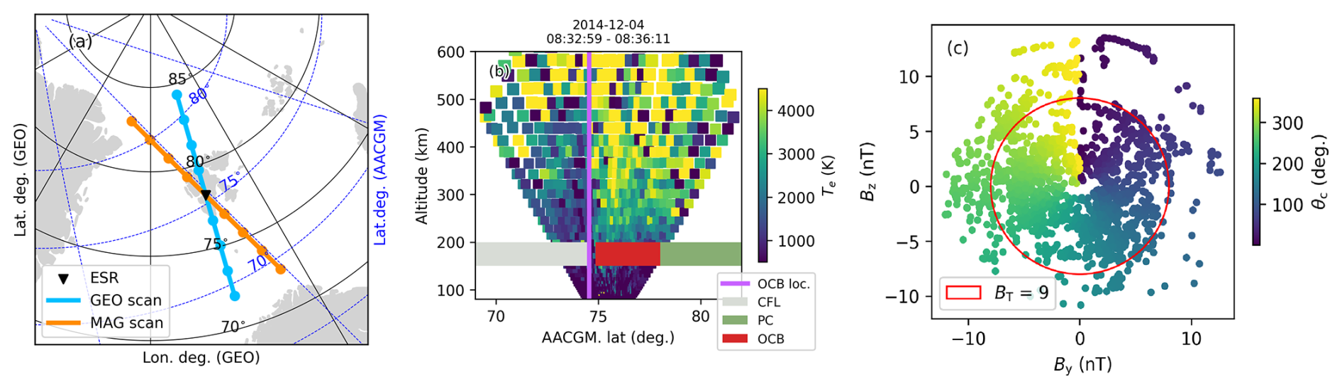
Figure 1 (a) Map of the ESR location outside Longyearbyen, Svalbard (black triangle) and the experiment geometries used for this study. The blue (orange) line shows the footprint of scans along the geometric (magnetic) meridians. The highlighted points show the FOV edges at 100, 200, 300, and 400 km altitude. Geographic coordinates shown in black, AACGM latitudes in dashed blue (Burrell et al., 2023; Shepherd, 2014). (b) Example ESR scan from 4 December 2014 showing T_e. The colored bands indicate the latitudes of the sections of the scan on closed field lines (CFL, gray), at the boundary edge (OCB, red) and in the polar cap (PC, green). The magenta line illustrates the open closed field line boundary. (c) The clock angle θ_c distribution for the data used in this study. The horizontal (vertical) axis corresponds to B_y (B_z) and the color scale to θ_c. The red circle highlights B_T = 9 nT.

In addition to the ESR observations, supplementary data was used. This includes solar wind magnetic field measurements from the OMNIWeb Database (King and Papitashvili, 2005, 2020), the auroral electrojet index (AE) from WDC Kyoto (Davis and Sugiura, 1966; World Data Center for Geomagnetism, Kyoto, et al., 2015), and the polar cap north (PCN) index from DTU Space at the Technical University of Denmark (Troshichev et al., 1988; World Data Center for Geomagnetism, Copenhagen, 2019). As the OMNI measurements are propagated to the bow shock, a delay is added to the IMF data to account for the delay time between the bow shock and the ionosphere. This added delay is 12 min (Samsonov et al., 2018).

Data selection

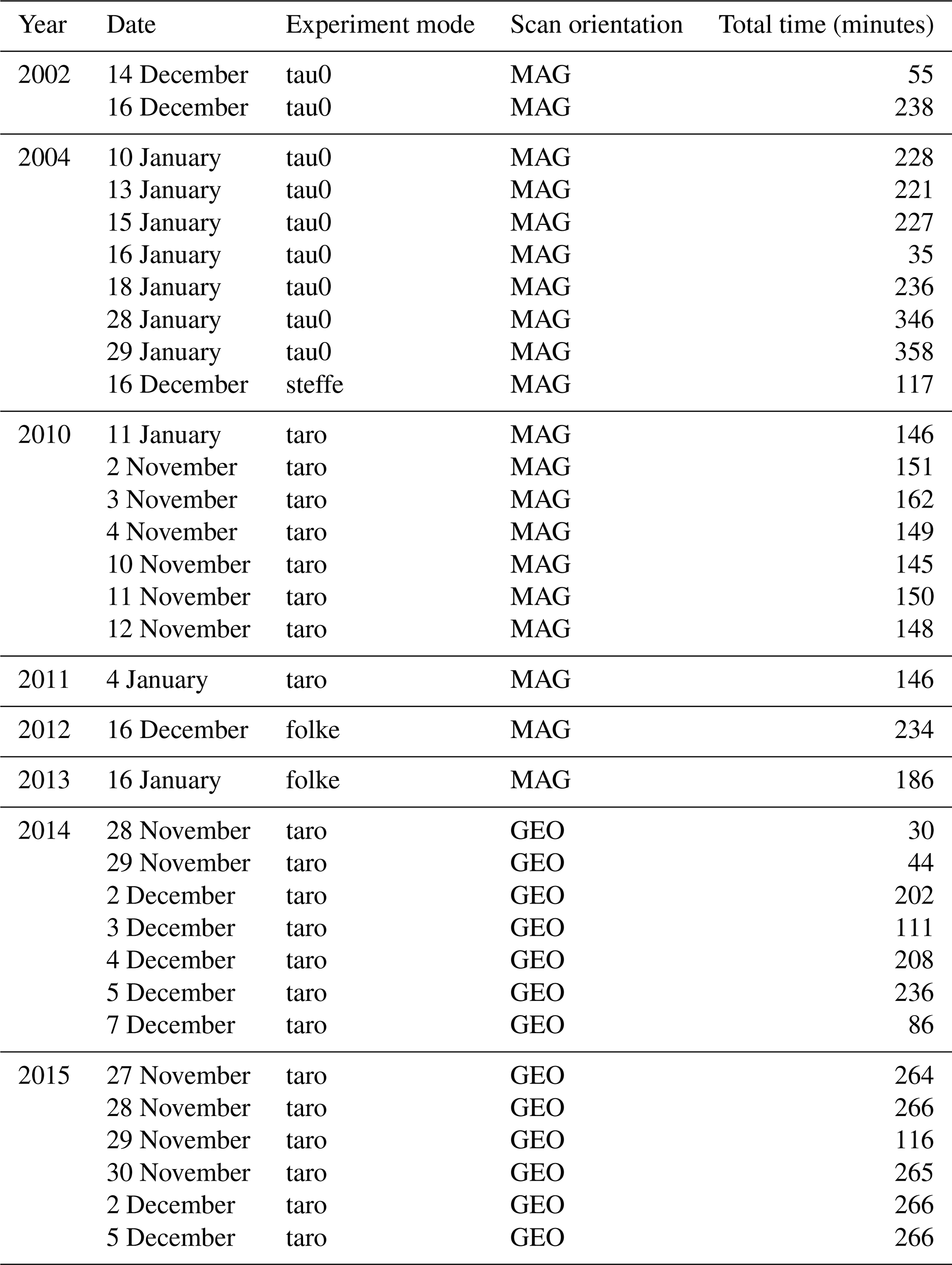
A total of 33 ESR scan experiments are used in this study, each run on separate days. The duration of the individual experiments ranges from 30 to 358 min. Combined, the 33 experiments consists of approximately 100 h of observations. Most of the experiments are centered at magnetic noon (local morning time for Longyearbyen), but the data also includes some pre-noon and post-noon observations. All experiments were run during the boreal winter, with the majority being from the winters of 2014 and 2015 (solar maxima), during 2002 (declining phase) or 2010 (solar minima). Information on the scans modes, orientations, and durations of each experiment are listed in Table A1. The data from each experiment was inspected visually, and the events with a clear auroral oval at 300 km were included in the data set used for this study.

3 Method

For identification of the dayside aurora in the ESR elevation scans, we use the method described by Frøystein et al. (2024). A short description of the method is given here. By running the ESR in a scanning mode, observations of the aurora and the quiet ionosphere can be made within a short time lapse. Using observations of T_e, N_e, and T_i within and outside the dayside aurora, the electron heating rate due to precipitation is estimated from the electron energy equation, and it is found that changes in N_e can introduce T_e variations of up to 1000 K given a constant heating rate. In addition, T_e falls off linearly with exponentially increasing N_e given a constant electron heating rate. This relation between T_e and N_e is then used to adjust an initial T_e enhancement threshold of 2000 K to include the N_e effect. Observations where this threshold is reached are classified as being within the dayside aurora or on open field lines.

For this study, we use the identified dayside auroral boundary to separate the ESR observations into three regions depending on their latitude relative to the boundary. Every point south of the boundary is classified as being on closed field lines (CFL). The region north of the boundary, which is on open field lines is split into two. A 3° band just northward of the boundary is classified as along the OCB (OCB) and the remaining points are classified as being in the polar cap (PC). To avoid possible classification errors between open and closed field lines, we add a 0.3° buffer band around the boundary latitude. This buffer is discarded. An example scan of T_e is shown in Fig. 1b. The magenta line shows the position of the OCB. The colored bands show the latitudes covered by each of the three classes.

Prior to conducting the statistical analysis, several steps are performed on the data. First, every ESR data point with a relative error greater than 30 % is discarded. The relative error is calculated as $|\mathrm{d}p/p|$ where p is the ionospheric parameter and dp is the error from the GUISDAP analysis. We assume that the ESR or GUISDAP errors are accounted for by doing this. The boundary method by Frøystein et al. (2024) also includes quality flags of the position of the latitude. Each obtained OCB latitude is flagged depending on the number of missing data points surrounding the location, the T_e threshold value dependence or lack of T_e gradients and the proximity to the ESR FOV edge. For the statistical analysis we omit all points flagged as “red”, which corresponds the most uncertain boundary location.

Finally, for the statistical analysis, we remove data points for which the IMF B_T>9 nT. This is done to ensure that the sampling is roughly even with respect to the IMF and therefore clock angle. This is illustrated in Fig. 1c), which shows the distribution of IMF B_y and B_z. Values below B_T<9 nT are relatively evenly distributed. On the other hand, values greater than 9 nT are skewed and including these points could introduce a bias in the results.

4 Results

This section first presents two case examples showing ESR observations for a detailed presentation of the time and latitude variation within the dayside auroral region. The two cases are chosen because they show (1) a clear dayside auroral region and (2) different IMF conditions, response, and morphology of the ionosphere. Next, statistical results of OCB latitude, as well as the altitude and latitude variation of the ionospheric parameters are presented.

4.1 Case 1: Latitude variation on 4 December 2014

Figure 2 shows ESR observations from 4 December 2014. The ESR was run in the taro experiment mode with the radar line of sight moving from 30° elevation pointing South to 30° pointing North, with every elevation step covering 6.4 s. This leads to full N–S scans over approximately 3 min. The shown parameters are the averages between 275–325 km over the different latitudes covered by the radar beam unless otherwise stated. For context, panels (a) and (b) show the IMF B_y and B_z components, and the AE and PCN indices, respectively. Panels (c)–(g) present parameters T_e, N_e,F, N_e,E (E-region, 110–130 km), T_i, and v_i, respectively. The velocity v_i is the horizontal component of the along-beam observed velocity. It is calculated from the observed velocity and the radar elevation angle. Velocities where the radar beam is almost vertical, from 85 to 95° elevation, are discarded.

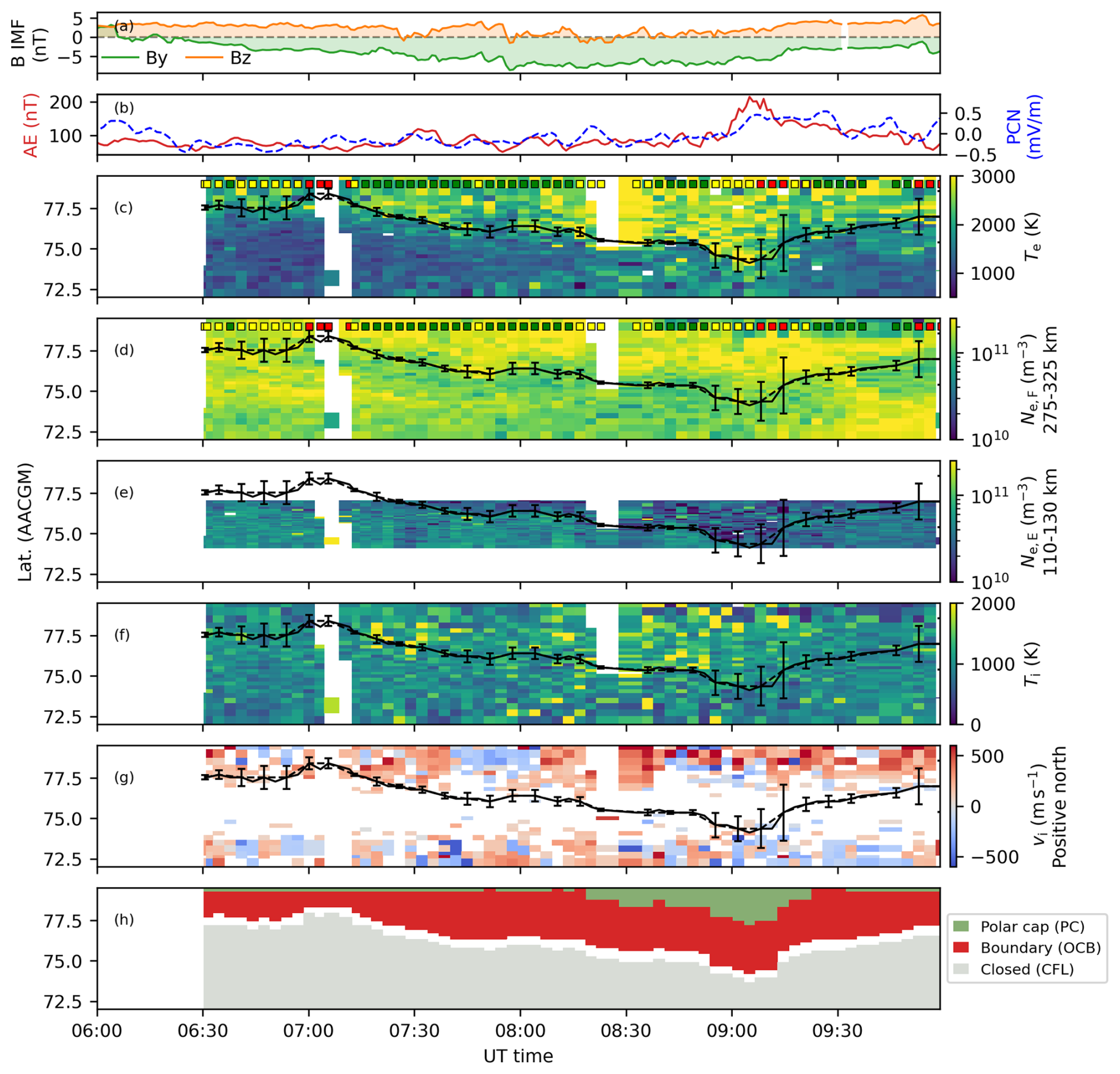
Figure 2 Overview of observed T_e, T_i, and N_e, and identified regions on open and closed field lines by the ESR 32 m from 4 December 2014. Panel (a) shows the IMF B_z and B_y components, panel (b) the AE (red solid, left hand axis) and PCN (blue dashed, right hand axis) indices, panels (c)–(g) show T_e, N_e,F (high F-region (275–325 km), N_e,E (E-region, 110–130 km), T_i, and v_i observed at 300 km altitude by the 32 m along the geographic meridian. The solid black line indicates the open-closed field line boundary. The colored squares show the quality flags. Panel (h) shows colored regions of the 32 m data corresponding to closed field lines (grey), in the polar cap (green) and along the open-closed field line boundary (red).

The open-closed field boundary based on the 32-meter observations is overlaid in black. The scattered squares colored in red, green or yellow are the OCB location quality flags for each time step. Panel (h) shows the identified regions, as illustrated in Fig. 1. Regions on closed field lines are colored in grey, the 3° band directly North of a 0.3° buffer in red shows the OCB region, and the polar cap region is drawn in green. The offset from UTC to MLT in Longyearbyen is approximately UTC+3 h. The shadow height at the ESR latitude is approximately 300 km at the beginning of the experiment and 120 km at the end of the experiment. The altitude is calculated using solar elevation angles from the PyEphem Python package (Rhodes, 2011).

For the case shown in Fig. 2, the IMF B_z and B_y are relatively stable and only the magnitude is slowly varying. B_z is positive throughout, save a few short intervals of low magnitude negative B_z in the middle of the experiment. B_y is negative throughout, except for some minor switches in the beginning of the experiment. The AE index, shown in panel (b), is low during the experiment, but reaches a peak of 200 nT slightly before 09:00 UTC. The PCN index is also relatively low throughout, but it increases slightly after 09:00 UTC.

The OCB is far North in the radar FOV at the beginning of the experiment, and gradually moves equatorward. The farthest South location is at 09:00 UTC, coinciding with the AE peak. After 09:00 UTC, the OCB retracts back towards the North of the radar FOV. The correlation coefficient between the OCB latitude and the AE index is −0.65. The OCB latitude error flags in Fig. 2c and d show that the boundary position is flagged as uncertain (“red”) where the position is found in a region of missing data, like shortly after 07:00 UTC. Similarly, the location is flagged as uncertain where the error bars in the latitude is large, e.g. shortly after 09:00 UTC.

As expected, T_e shown in panel (c) is enhanced along the identified boundary and the gradient from closed to open field lines is generally well defined. During intervals where the gradient is not well defined, the boundary latitude is flagged as uncertain, e.g. at approximately 09:00 UTC. In addition, the enhancements in T_e are clear during the entire experiment and span several degrees in latitude. In particular, no differences between the OCB region and the PC are visible here. The enhancements appear to peak between 08:00–09:00 UTC. This collocates with the AE maximum.

N_e in the F-region, shown in panel (d), is relatively stable throughout but there is a region of slightly lower density on closed field lines in the middle of the experiment. Toward the end of the experiment there is an increase in N_e at the Southward edge of the radar FOV which creeps Northward. N_e,E, shown in panel (e), is slightly higher in the first half of the experiment. On open field lines, the density is lower, but the difference is not striking.

T_i, shown in panel (f), exhibits intermittent enhancements. However, the enhancements are not as clear and as persistent in time as the T_e enhancements. The region of most clearly and evenly enhanced T_i coincides with the peak T_e between 08:00–09:00 UTC. There is also an enhanced region between 07:00–07:30 UTC along the OCB and a region at the equatorward edge of the FOV at 08:00 UTC.

Although the measurements are very noisy, there are some patterns in v_i (panel g). For example, there is a region of reverse flow shortly after 07:30 UTC.

4.2 Case 2: Latitude variation on 5 December 2015

Figure 3 shows ESR observations from 5 December 2015 (in the same format as the case shown in Fig. 2).

Figure 3 Same as Fig. 2 for 5 December 2015.

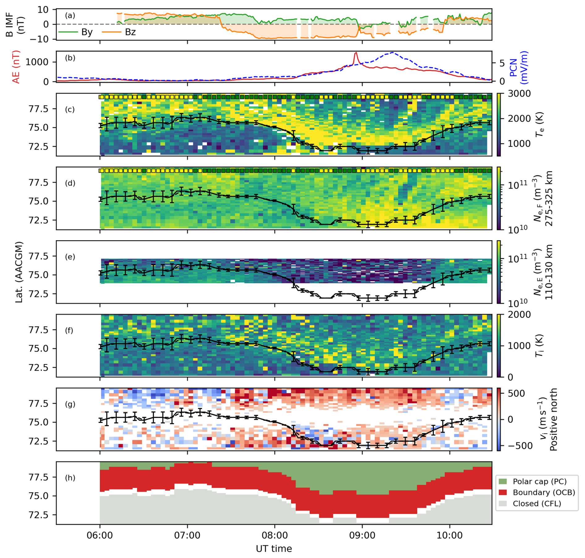
For the December 2015 experiment, B_y, shown in panel (a), is consistently positive, except for some short intervals prior to and after 09:00 UTC. B_z is positive until about 07:15 UTC before turning southward, reaching values of up to −10 nT. B_z remains negative until shortly before 10:00 UTC, save for a slight switch at 09:00 UTC. The AE index, shown in panel (b), is low and stable until about 08:00 UTC, growing slowly before a sharp and short-lived peak before 09:00 UTC. While remaining high for the rest of the experiment, it decays slowly toward the experiment end. The PC index increases steadily from 08:00 UTC and reaches its peak at ∼09:15 UTC. The shadow height at the ESR latitude is approximately 340 km at the beginning of the experiment and 115 km at the end of the experiment.

The OCB, which is plotted over the ESR parameters in panels (c)–(g), is almost directly overhead at the beginning of the experiment, before propagating toward the South edge of the FOV following the southward turning of the IMF. However, there is a ∼20 min delay before the OCB starts moving. The OCB latitude is low until about 09:30 UTC before retracting. Around this time the IMF turns northward. As for the 2014 case, the OCB seems to be inversely linked to both the AE and PCN indices, where the largest AE values coincides with the lowest OCB latitudes. In fact, the correlation coefficient between the OCB latitude and the AE index is −0.91.

The enhancements in T_e (shown in panel c) on open field lines have a wide peak centered at approximately 08:20 UTC. After 08:20 UTC and until approximately 09:30 UTC, there is a strong N–S T_e gradient from the region on CF to the OCB region while there is a softer gradient northward of the T_e enhancements into the polar cap. During this interval, there are also several Polar Moving Auroral Forms (PMAFs). These are seen as defined structures of enhanced T_e that move poleward (Northward).

N_e is stable throughout, save for some patchy activity and a depletion around 09:00 UTC. In the E-region, shown in panel (e), N_e is highest at the start and the end of the experiment. There is a clear reduction as the IMF turns Southward and the OCB moves southward. Toward the end of the experiment the density again increases.

There is a more clearly defined region of enhanced T_i than for the December 2014 case. From 07:30 UTC to about 09:20 UTC there is a clear band of enhanced T_i, although it is less even than the T_e band. Some other regions of enhanced T_i, e.g. before 07:00 UTC and after 09:30 UTC, are also seen. There are several points of interest in v_i. Following the turning of the IMF, its magnitude increases and the velocity is clearly poleward. At the location of the highest T_e and T_i, and coincident with the 4th PMAF at 10:00 UTC, there are pockets of reversed flow.

Following the southward turning of the IMF at approximately 07:15 UTC, several features are observed in the ESR measurements. For T_e, the strength of the S-N gradient across the OCB increases. The enhancements in T_i increase. v_i is strongly northward from the southward turning, and until the IMF northward turning. These three features are observed just after the southward turning at 07:15 UTC. The OCB moves equatorward following the southward turning, but the movement only starts ∼20 min after the turning and the features are observed in the ESR parameters.

To summarize, this section has presented two case studies that show different IMF conditions and ionospheric responses. The key difference is that the 2015 case (Fig. 3) contains a strong southward turning of the IMF and the ionosphere is more structured, with both patchy N_e and PMAFs.

4.3 Open-closed field line boundary location

For completeness, this section presents a statistical analysis of the location of the OCB. The location and movement of the OCB is linked to the opening of magnetic flux at the dayside magnetopause and to the closing of flux in the magnetotail, and its latitude is therefore expected to relate to both the IMF and geomagnetic indices such as AE (Lockwood et al., 2005, references therein). This is previously shown in studies based on ASI (Johnsen and Lorentzen, 2012b) and satellite (e.g. Newell et al., 1989, 2006). Here, we therefore investigate the relation of the OCB latitudes obtained by the ISR method to the IMF B_z component, the AE, and PCN indices and to a coupling function (Newell et al., 2007).

Figure 4 shows the boundary latitude obtained by the radar method. The latitudes are shown as a function of $\mathrm{d}{\mathrm{\Phi }}_{\text{MP}}/\mathrm{d}t$ which represents the change in open magnetospheric flux (Newell et al., 2007), the AE (Davis and Sugiura, 1966) and PCN (Troshichev et al., 1988) indices, and the IMF B_z component. Only data points where 11:00 < MLT < 13 are included as the cusp is most likely within this interval (Newell et al., 1989).

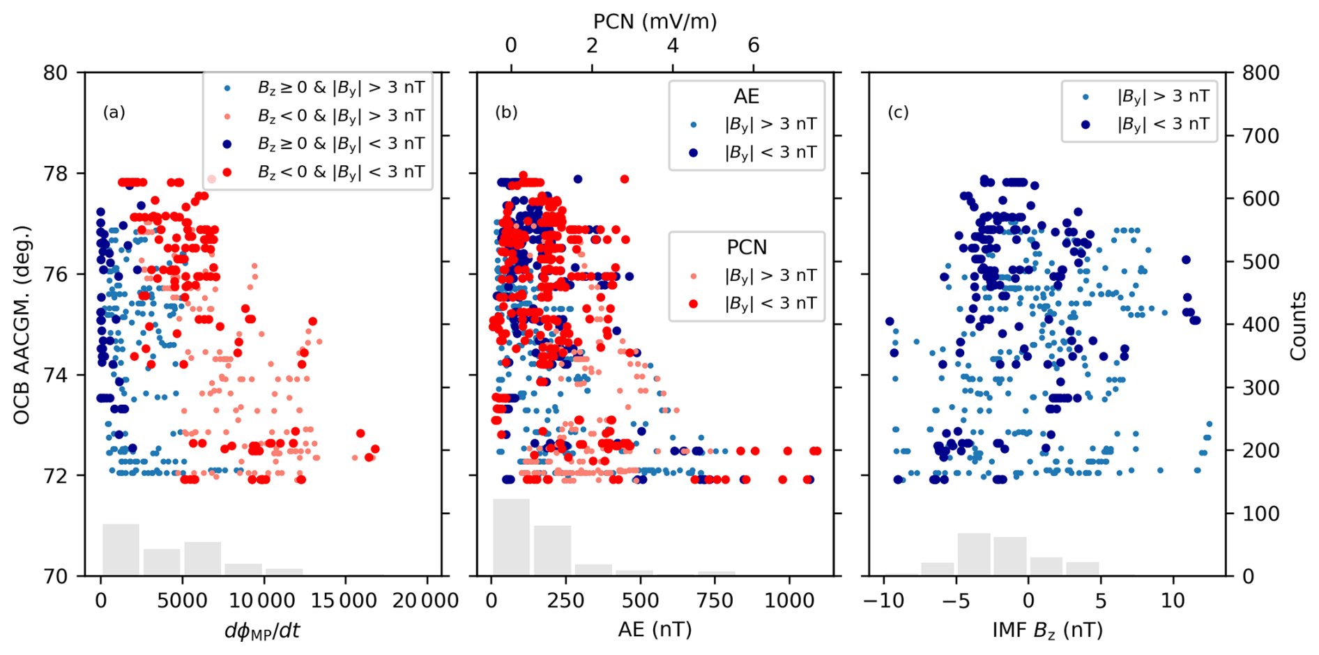
Figure 4 Obtained OCB latitude plotted with respect to (a) coupling function $\mathrm{d}{\mathrm{\Phi }}_{\text{MP}}/\mathrm{d}t$ (Newell et al., 2007), (b) the AE index (Davis and Sugiura, 1966), and the PCN index (Troshichev et al., 1988), and (c) IMF B_z. The grey histograms (right hand axes) show the distribution of points binned by either three parameters. In panel (a), the red (blue) dots show $\mathrm{d}{\mathrm{\Phi }}_{\text{MP}}/\mathrm{d}t$ for negative (positive) B_z. In panel (b), the red dots are with PCN, the blue points with AE. The lower (upper) horizontal axis shows AE (PCN). For all panels, the smaller and lighter colored dots are for $\left|B_y\right|>\mathrm{3}$ nT, and the darker dots are for $\left|B_y\right|<\mathrm{3}$ nT.

In Fig. 4 a, the red dots indicate where B_z≤0 nT and the blue dots where B_z>0 nT. In panel (b), blue dots indicate points sorted with respect to the AE index, the red dots with PCN. For all three plots (panels a–c), large points mark data points where $\left|B_y\right|<\mathrm{3}$ nT. Small and more lightly colored points have $\left|B_y\right|>\mathrm{3}$ nT. The right-hand axis shows the number of points per interval on the horizontal axis. Points where the OCB latitude is flagged as uncertain are removed.

Although the distributions of latitudes are widespread and clearly limited by the narrow ESR field of view, some trends are visible. For both the AE index and $\mathrm{d}{\mathrm{\Phi }}_{\text{MP}}/\mathrm{d}t$, the variation in the OCB latitude is larger for the smallest values, spanning the entire range of the radar FOV. For larger AE, especially above 500 nT, no OCB latitudes above 75° are detected. The same trend is seen in $\mathrm{d}{\mathrm{\Phi }}_{\text{MP}}/\mathrm{d}t$. Larger index values yield a smaller range of latitudes, shifted towards the equatorward edge of the radar FOV. This is true for both large and negligible $\left|B_y\right|$.

For IMF B_z (panel c) the trend is similar, but weaker. For B_z>0 nT, the spread in latitude is large. For B_z>5 nT and $\left|B_y\right|<\mathrm{3}$ nT, there is a preference for higher latitudes, but the number of points in this range is low. For B_z<0 nT, the latitudes are lower for both small and large $\left|B_y\right|$ nT. For B_z>0 nT and B_y>3 nT, there are also a number of data points with lower latitudes. This population disappears when considering only $\left|B_y\right|<\mathrm{3}$ nT. Overall, the obtained OCB latitudes behave in the same manner as has been presented in previous studies (Newell et al., 1989, 2006; Johnsen and Lorentzen, 2012b), although our data set is smaller and there are some limitations concerning the FOV.

4.4 Statistical altitude profiles by region

For an overview of the variation in T_e, T_i, and N_e, this section presents a statistical analysis of the three parameters in the three regions CFL, OCB, and PC.

Using elevation scans makes it possible to observe both latitudinal and altitudinal variation of the ionospheric parameters within ∼3 min. Accordingly, the altitudinal variation can be investigated separately. In this section, we present a quantitative analysis of the variation between the three regions, CFL, OCB, and PC, by constructing average altitude profiles within each region. Prior to constructing the profiles, the data is filtered by a median filter with kernel size 3. This is done for the statistical results in this section and further sections.

Figure 5 shows an overview of T_e, N_e, and T_i shown as altitude profiles in the three regions. The medians for each altitude bin for each region make up the the altitude profiles in the left column. The middle column shows the distributions of each parameter for every 30 km altitude bin for each region. The distributions are centered at the median for each altitude bin. The right hand column shows the number of points contributing to the altitude bin median and distribution in each altitude bin. The distributions for all three parameters include some amount of unreasonable outliers. Therefore, the error estimates for each altitude range are calculated as the 30th and 70th percentiles of the distributions.

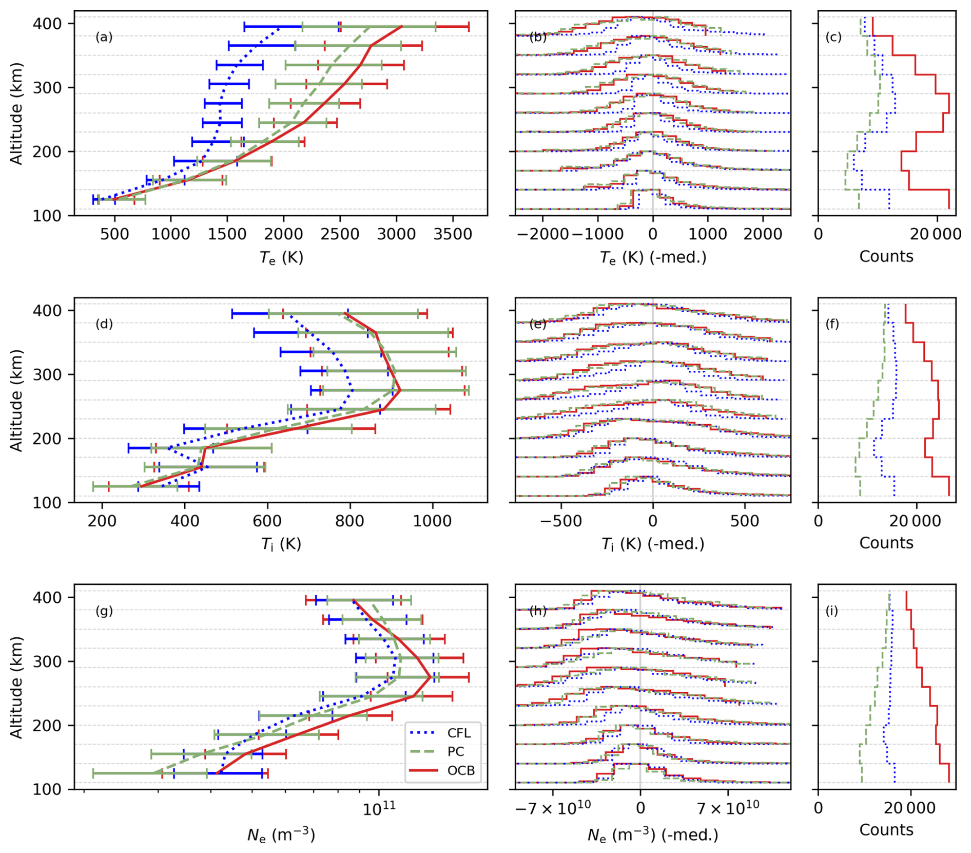
Figure 5 Altitude profiles (left), normalized histograms of variations in each 30 km altitude range (middle) and histograms showing the number of points per region and altitude range (right). Each row shows T_e, T_i, and N_e, respectively. Profiles corresponding to each region is drawn in dotted blue (CFL), dashed green (PC) and solid red (OCB) curves. The errorbars for each altitude range of the profiles (left) correspond to the 30th and 70th percentiles of the corresponding distributions (middle). Only points were $\left|B_{\mathrm{T}}\right|$ < 9 nT and 09:30 < MLT < 14:30 are included.

From Fig. 5a, it appears that the T_e difference between CFL and along the OCB increase with altitude, especially above 200 km. The increase peaks upwards from 300 km with a difference of 900–1000 K from the closed field lines, corresponding to a factor of 1.5–1.6. Although the error bars are large and the distributions are wide, it appears that T_e is hotter along the OCB than in the PC above 200 km. Above 300 km, the median is on average ∼200 K degrees hotter along the OCB than in the PC.

A similar trend is seen in T_i (panel d), where an increase from closed to open field lines above approximately 170 km altitude is seen. From around 260 km and upwards, the increase from CFL to open field lines (OFL) averages to 120 K and varies little with altitude, corresponding to a factor increase by 1.1–1.2. There are no distinguishable differences between the OCB and the PC.

For N_e in panel (g), there is a clear increase along the OCB centered at around 280 km altitude. Between 170–300 km N_e along the OCB reaches densities over 1.3×10¹¹ m³, with an increase from CFL to the OCB by a factor 1.1–1.4. In the PC, the density is lower than along the OCB across all altitudes except at the top altitudes. The PC densities are slightly higher than the CFL densities, except at the lowest altitudes.

4.5 Latitude variation relative to the OCB

For a more detailed look at the latitude variation of the parameters, Fig. 6 shows a superposed epoch analysis of T_e (top row), T_i, and N_e (bottom row) with respect to the OCB, allowing to study how the quantities vary with distance from the OCB.

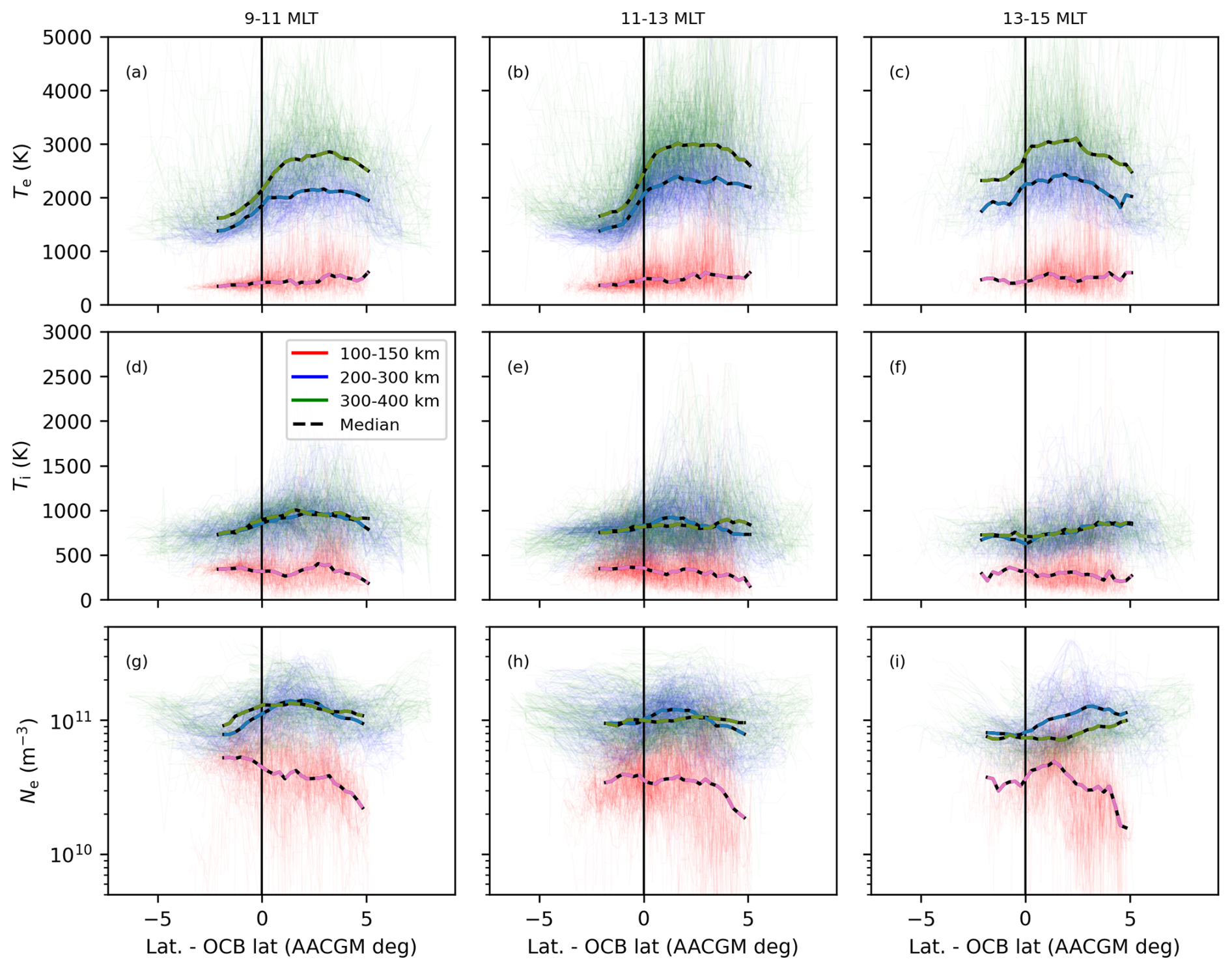
Figure 6 Variation of the ionospheric parameters relative to the OCB. Panels (a)–(c) show T_e from 09:00–11:00, 11:00–13:00, and 13:00–15:00 MLT, respectively. Panels (d)–(f) show T_i and (g)–(i) N_e. The red lines show altitudes 100–150 km, the blue 200–300 km and the green 300–400 km. The dashed colored and black lines shows the median for the corresponding altitude. The black vertical line show the OCB (0° offset).

The groups of red, blue and green lines correspond to the ionospheric parameters on altitude intervals 100–150, 200–300 and 300–400 km. The data points are extracted from altitude cuts like the ones in Figs. 2 and 3. Each altitude cut is the average over 25 km. The colored-black dashed lines show the median for each altitude range. The horizontal axis shows the latitude offset (AACGM degrees) from the OCB. Each column shows a specific time interval. The left column shows interval 09:00–11:00 MLT, the middle column shows interval 11:00–13:00 MLT, and the right column shows 13:00–15:00 MLT.

As seen in panels (a)–(c), the F-region T_e exhibits clear variations with respect to latitude relative to the OCB regardless of the time interval. Most striking is the strength of the T_e gradient across the OCB. The gradient when crossing the OCB is significantly steeper for the 11:00–13:00 MLT interval than for the two other intervals. For 11:00–13:00 MLT, T_e is enhanced until 4° poleward of the OCB before decreasing. For all three time intervals, the spread in the F-region T_e is larger poleward of the OCB. Between 100–150 km altitude, the variation in T_e relative to the OCB is negligible expect for a larger spread poleward of the OCB.

For T_i shown in panels (d)–(f), there are also some differences dependent on the relative distance to the OCB. Although T_i also increase poleward of the OCB, no strong latitudinal gradient such as the one seen in T_e can be observed.

In the F-region, T_i is slightly enhanced on open field lines. Latitudinal variation apart from this enhancement is hard to discern although there might be some differences between the three MLT ranges. For all three intervals, there is a significant difference in the standard deviation between open and closed field lines. On open field lines, poleward of the OCB, the standard deviation is significantly enhanced. Between 13:00–15:00 MLT there is little to no latitudinal variation in T_i.

The behavior of the F-region N_e (panels g–i) is different between the three intervals. For 09:00–11:00 MLT, the N_e peaks poleward of the OCB and decreases gradually into the polar cap. For 11:00–13:00 MLT there is a less pronounced peak and N_e decreases gradually from the equatorward edge of the FOV to the poleward edge. For 13:00–15:00 MLT there is a stronger difference between 200–300 and 300–400 altitude ranges, and it peaks just poleward of the OCB between 200–300 km altitude. In the E-region, there is a pronounced decrease in N_e on open field lines. For 13:00–15:00 MLT, there is a slight peak in N_e just northward of the OCB. For all three time intervals, the lowest E region N_e values are poleward of the OCB.

4.6 Electron density variation in E and F regions

To further characterize N_e in the dayside ionosphere, this section presents an analysis of the N_e variation in the E and F regions. The electron densities in the E and F regions depend on different precipitation energies and therefore contain information about the precipitation into the dayside auroral region. Their time variation or relationship can both be used to gather information about said precipitation (e.g. Skjæveland et al., 2017). In this section the N_e,E to N_e,F ratio is quantified for the scans used in this study, which may provide information on the ratio of high to low energy precipitation.

Figure 7 shows the ratio between N_e,E to N_e,F as a function of MLT for the PC (panel a), OCB (panel b) and CFL (panel c). For each timestep, average N_e values in the E and F regions are calculated in the CFL, OCB, and PC regions. To account for the FOV size differences between high and low altitudes, the F region N_e is cropped to match the E-region FOV before the averages are calculated. The colored points show the hourly median. The last binned median is on the interval 13:00–14:00 MLT. This is because the number of points in the next two bins is low, especially for the CFL and PC regions. For completeness, the number of points per MLT hour interval is also plotted using dashed black bars.

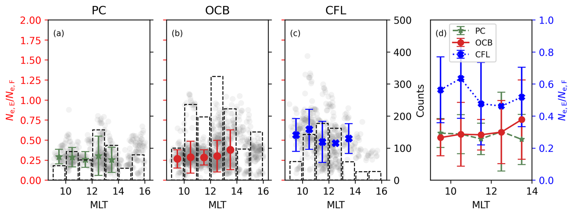
Figure 7 Ratio between N_e in the E region (110–130 km) and in the F region (200–300) in the (a) PC, (b) OCB, and (c) CFL regions. The gray points are all points of the ratio wtr. MLT. The colored points are the binned averages per full hour. The error bars show the standard deviation in the bin. Panel (d) shows the binned averages in all three regions.

Even though the FOV is limited in the E region and the spread in the data is naturally relatively large, some trends with respect to MLT can be perceived. The behavior of the N_e ratio is different between the three regions.

On CFL, the ratio peaks pre-noon at values up to 0.6. After 11:00 MLT the ratio varies little around approximately 0.5. On open field lines (OCB and PC) the ratio is almost constant with MLT, and any MLT variation is far within the error bars. The ratios averages at almost 0.3.

Larger ratios are explained by either larger E region densities or lower F region densities. In general, larger ratios are more likely on CFL than on open field lines regardless of MLT range.

5 Discussion

In this work we performed a quantitative analysis of the behavior of plasma parameters T_e, T_i, and N_e in the polar dayside ionosphere. We showed two case examples that illustrate the dynamic response of the ionosphere to the solar wind. Further, we performed statistical and superposed epoch analyses of how the before-mentioned parameters vary with respect to altitude and with the distance to the OCB.

5.1 Case examples and IMF impact

The case examples show aspects of the dynamic behavior of the dayside auroral region. The regions of enhanced T_e clearly display the presence of low energy precipitation. The 2015 event (Fig. 3) exhibits a southward turning and shows signatures of pulsed magnetopause reconnection. Indeed, after 08:00 UTC, several PMAFs appear. PMAFs are typically related to flux transfer events in the dayside magnetopause (McCrea et al., 2000; Lockwood et al., 2000, references therein). The intensity of the PMAFs and the time intervals between them vary, which is consistent with previous observations (Lockwood et al., 1993). Strong latitudinal T_e gradients such as the one seen after ∼07:30 UTC in Fig. 3d, has also been linked to the cusp (Nilsson et al., 1996). There is also a strong enhancement of the poleward flow velocity in v_i, which can be linked to reconnection. In the 2014 case in Fig. 2, where the IMF is positive throughout, less structured behavior and fewer signatures associated with magnetopause reconnection are seen.

In the 2015 case in Fig. 3, the OCB moves equatorward following the southward turning of the IMF, which can be explained by reconnection at the magnetopause which expands the region of open field lines equatorward. After the IMF turns northward, the OCB relaxes poleward. In the 2014 case, the OCB also moves equatorward, which can be explained by growing convection cell size due to the considerable B_y component (Milan et al., 2003). This is also seen in the OCB statistics in Fig. 4c, where both B_z and B_y affect the latitude.

Between the two presented cases, there seems to be less structured behavior in all four ionospheric parameters for positive B_z, especially in T_e and N_e. The two cases differ most after the southward turning, where we observe highly structured T_e, N_e, and an increased v_i in the 2015 case (Fig. 3). Similar trends were observed by McCrea et al. (2000) in field aligned ESR observations. This is also seen in several of the other experiments in Table A1, especially in cases with well-defined intervals of stable southward or northward IMF. Although common, not all of the experiments match this description, which helps illustrate the dynamic nature of the dayside auroral ionosphere, and challenges in predicting its behavior. It is also worth mentioning that directly comparing the ionosphere to IMF observations at Lagrange point 1 can be influenced by the variation of the spacecraft relative position to the Sun–Earth (S–E) line and the time delay from the bow shock to the ionosphere (Milan et al., 2022). Therefore, exact characteristics of the solar wind and IMF that reach the magnetopause can be uncertain. Although this effect is not large, small uncertainties concerning IMF effects can be introduced. For instance, for the 2015 case (Fig. 3), the NASA Magnetospheric Multiscale Mission (MMS) satellites crossed the S–E line during the experiment (seen in MMS orbit plot from https://lasp.colorado.edu/mms/sdc/public/plots/#/historical-orbit, last access: 8 April 2026). The MMS observed IMF exhibits overall similar characteristics to that of the OMNI dataset, including the timing of the Southward turning; however, some small variations can be perceived (seen in MMS quick look plots at https://lasp.colorado.edu/mms/sdc/public/plots/#/quicklook, last access: 8 April 2026). A more detailed analysis of the effect of such variations between IMF observations at different positions along the S–E line and ESR measurements could be interesting, but it is outside the scope of this study.

5.2 Statistical analysis

Figures 5 and 6 shows statistical results considering T_e, N_e, and T_i. Before these results are discussed, four aspects of the statistical analysis are addressed in the following four paragraphs.

First, T_e is the main parameter used in the method for obtaining the OCB latitude and for separating open from closed field lines. Therefore, a separation between open and closed field lines and higher T_e on open field lines is expected. However, T_e is the parameter exhibiting the strongest latitudinal differences between open/closed field lines when viewing the experiment observations separately (e.g. Figs. 2 and 3). In the superposed epoch analysis, we also note that the OCB is typically placed where the T_e gradient is strongest. Further, every timestep where the latitude of the OCB is uncertain is not included in the statistics.

Secondly, for this study, the regions of interest were defined to primarily separate the ionosphere on open field lines and closed field lines, and to distinguish the region closest to the OCB from the remaining open field lines. The region closest to the OCB contains possible cusp passes and possible reconnection signatures due to its proximity to the OCB. It is also likely that cusp passes are classified in our PC region if the cusp is more than 3° wide in latitude, which is not uncommon (Newell et al., 2006; Wing et al., 2001). In addition, our OCB region likely contains ionosphere in the polar cap. The size of the cusp is dynamic and separating it from the remaining open field lines is not straightforward. However, the altitude profiles do not vary significantly when varying the separation latitude (OCB + 3°) between the OCB and PC regions.

Next, the velocity v_i was omitted from the statistical analyses. Due to the nature of elevation scans, the observed line of sight v_i is a mixture of vertical and horizontal velocities depending on the current elevation angle. When calculating the horizontal N–S v_i, data is lost overhead the radar and emphasis is therefore put on the edges on the FOV. This is especially critical for the E-region, where the FOV is narrow. In addition, depending on the ESR position relative to the convection pattern, the magnitude of N–S and E–W velocities will vary (Moen et al., 2001). Since the data set includes experiments along both the geographic and geomagnetic meridians, the interpretation of what parallel velocity that is observed is slightly different (magnetic or geographic N–S).

Finally, attempts to quantitatively assess v_i proved difficult due to a large number of unreasonably high values in the E-region and a high sensitivity to the treatment and filtering of the observations prior to quantification. This sensitivity indicates that any possibly obtained trends in v_i would be too uncertain. On the other hand, this sensitivity was not observed in the remaining ionospheric parameters.

Despite the challenges above mentioned, Fig. 5 showed differences between the ionospheric parameters on open (OCB, PC) and closed field lines along the altitudinal column. The differences are, as expected, most clear in T_e. However, possible trends are also seen in N_e and T_i.

Simultaneous signatures in both N_e and T_e have been used to identify the cusp region in ISR data, e.g. by thresholds such as T_e>3000 K and $N_{\mathrm{e}}>\mathrm{3}\times {\mathrm{10}}^{\mathrm{11}}$ m⁻³ above 300 km (Nishimura et al., 2021). These values are significantly larger than the average values in the statistical altitude profiles in Fig. 5. There is enhanced N_e along the OCB where the cusp precipitation is expected to enhance N_e at 280 km, but values of 3×10¹¹ m⁻³ are rare and accounts only for 4.3 % of all N_e values in the OCB region and 2.6 % in the PC at 300 km. In addition, these percentages are elevated by days were the electron density is generally high. Jin et al. (2023) use a threshold of 1800 K for T_e when identifying the dayside auroral region. This threshold agrees well with the separation between T_e on CFL and along the OCB in our dataset. The ESR data based electron heating model in Frøystein et al. (2024) suggests that electrons heated by precipitation on open field lines are separated from cool electrons on closed field lines at approximately 2000 K. This also fits the presented separation.

In their model study, Vontrat-Reberac et al. (2001) predict strongly enhanced T_e reaching up to 1000 K peaking at around 300 km due to cusp precipitation. The expected T_e are significantly lower for boundary layer precipitation, only a few ∼100 K. Our observed enhancements of up to 1000 K is in agreement with these values, which might indicate that a large fraction of our observations contain cusp precipitation. Almost 65 % of the data points in this study is within the interval 10:30–13:30 MLT which is the most probable MLT range for cusp observation (Newell et al., 1989).

In their study, Lockwood et al. (2000) observe altitude profiles of the ionospheric parameters within the cusp, the polar cap and equatorward of the dayside aurora with the ESR looking field aligned. However, their altitude profiles are not measured simultaneously and are separated by up to 30 min and contains only a few minutes of data each. They observe T_e enhanced in the cusp region that are significantly higher than the temperatures in Fig. 5 at above 3500 K at 400 km altitude. They observe lower temperatures in the polar cap than in the cusp, at even lower values than the sub-auroral T_e. Although the magnitudes differ, the results presented in Fig. 5 are similar and support these previous observations.

For the latitude variation, several points of interest are seen in Fig. 6. The enhancements in T_e in panels (a)–(c) are wide with respect to latitude poleward of the OCB in the F-region. The width of the enhancements are slightly larger than what is expected of the cusp (Newell et al., 2006; Wing et al., 2001). For the interval 11:00–13:00 MLT, the equatorward T_e gradient is the strongest. This is a cusp signature (Nilsson et al., 1996), consistent with strong anti-sunward flow of cool plasma recombining with heated plasma below the cusp. The fact that there is little to no visible latitude effects in the E-region T_e is explainable by considering that the low energy precipitation that heats the F-region electrons on open field lines does not reach E-region altitudes.

The increased variation in T_i on open field lines in Fig. 6d–f matches the observations in the presented case examples, i.e. that the enhancements in T_i are more sporadic than T_e. Enhancements in T_i is also not necessarily coincident with T_e enhancements, which is also observed by Nilsson et al. (1996). Increases in T_i are heavily linked to enhanced Joule heating rates that are linked to increased flows (e.g. Moen et al., 2004), meaning that v_i is likely enhanced where T_i is high. The increased variability in T_i on open field lines would be worthwhile a more detailed look in a future study.

The investigation of N_e in the E-region compared to the F-region (Fig. 7) showed that there are slight MLT trends on CFL. The ratio decreases after 11:00 MLT. A small ratio signifies that the E-region is less dense or the F region density is larger. This scenario can be explained by low energy precipitation into a dark ionosphere, consistent with dayside precipitation from either the cusp or mantle (Newell et al., 2004). Low energy precipitation does not penetrate into the E-region, which is depleted due to a lack of ionization in the dark ionosphere. The precipitation rather increases the density in the F-region. This process is used for identification of the cusp (e.g. Skjæveland et al., 2017), where the cusp is found in regions with a depleted E region coincident with an enhanced F region N_e. Skjæveland et al. (2017) use conditions on both the E and F region densities when identifying the cusp.

Although the error estimates and variation per MLT bin in our analysis are large, the trends are as expected. Denser E-regions are more likely on closed field lines especially pre-noon due a larger amount of higher energy precipitation on closed field lines pre-noon than compared to post-noon (Newell et al., 2004). In addition, there is a larger amount of ionization due to solar EUV post-noon (09:00 UTC). The effect of EUV ionization is largest in the F-region, but after noon, the shadow height is below 100 km altitude in the southern part of the ESR FOV. In Fig. 2 there is an increase of N_e at the equatorward edge of the FOV after 09:00 UTC that grows poleward. The F-region N_e can also be affected by structures such as patches, which can influence the comparisons.

6 Conclusions

The dayside auroral ionosphere is a dynamic region which is strongly affected by the solar wind-magnetosphere-ionosphere coupling. Several important ionospheric quantities, such as conductivities (Maeda, 1977), rely on how the ionosphere varies due to this coupling. Characterizing the behavior of the dayside auroral ionosphere is therefore valuable. In this paper, we have presented a quantitative analysis of the behavior of the ionospheric plasma parameters observed by ESR elevation scanning experiments. From the scans, the open-closed field line boundary (OCB) latitude was identified and the ionosphere was classified into three regions relative to the OCB. In addition to two case studies, we have presented statistical and superposed epoch analyses to investigate the variation with altitude and to the distance to the OCB. The presented case studies are highly different with respect to both the IMF conditions and the ionospheric behavior, and illustrate the dynamic nature of the region. For the two events, the ionosphere appears to be more stable for positive B_z, whereas for negative B_z the ionosphere is more structured and dynamic. Observed effects include patchy electron density N_e (Carlson, 2012) and polar moving auroral forms (Lockwood et al., 1993).

The statistical results show differences between the three regions. First, the ionospheric F-region electron temperature enhancements within the dayside auroral oval peak above 300 km with 1000 K. The enhancements are strongest in the OCB region and extend for several degrees in latitude poleward of the OCB latitude. Both the poleward T_e gradient across the OCB and the T_e values maximize at noon MLT, which corresponds to the time interval most likely containing the cusp. On average, N_e has a defined peak in the OCB region just below 300 km altitude, consistent with enhancements due to low energy precipitation. In the E-region, below that altitudes at which low energy precipitation typically deposit their energy (Mantas and Walker, 1976; Millward et al., 1999; Vontrat-Reberac et al., 2001), the density decreases slightly with increasing latitude into the polar cap. The observed ratio between N_e in the E and F regions is larger on closed than on open field lines, indicative of higher energy precipitation in the former region. For T_i, the variability maximizes on open field lines, although the average values only increase slightly across the OCB.

To extend the statistical analysis, it could be beneficial to include field-aligned ESR observations. This would require a method modification, but would greatly increase the data set size and allow for investigation of larger temporal trends and solar cycle trends. In addition, future observations based on the current ESR, or even a new system would be valuable (Baddeley et al., 2023). Nevertheless, the current data set based on ESR elevation scans made it possible to present a study characterizing the dynamic nature of the dayside auroral region with respect to both altitude and latitude.

Appendix A: Table of ESR experiments

Table A1 Experiment modes (3rd column), scan orientations (4th column) and total time in minutes (5th column) of the 33 experiments used in this study.