New technique for isolating the auroral contribution in UV imagery: IMF B_y dependence of seasonal differences in auroral oval location during positive IMF B_z

We investigate how the location, size, and intensity of the auroral oval is affected by the combination of the tilt of the Earth's magnetic dipole axis and a strong, stable dawn/dusk component of the interplanetary magnetic field (IMF B_y) during northward IMF. Sunlit auroral observations are contaminated by dayglow, and its impact on average intensity estimates remains unclear. Dayglow modelling is also accompanied by significant uncertainties that increase with increasing sunlight intensity. These difficulties motivate us to develop a new technique for isolating the auroral contribution in dayglow-subtracted UV images. This technique assumes the observed distribution of intensities consists of separate contributions from dayglow and aurora, and that the dayglow subtraction process to which the observations are subjected is imperfect and leaves a residual error. By performing a nonlinear fit to dayglow-subtracted count distributions one may extract the best-fit parameters that describe the dayglow residual error and auroral sources separately. We apply this isolation technique to dayglow-subtracted UV images derived from measurements made by the Special Sensor Ultraviolet Spectrographic Imager (SSUSI) onboard the Defense Meteorological Satellite Program’s F16–19 satellites during 2005–2018. The isolation technique produces 30 %–40 % higher auroral intensities than a simple calculation of the distribution mean. Statistics of the auroral component show a clear and substantial (∼500 km in NH, ∼430 km in SH) dawn-dusk shift in the polar cap location depending on the sign of IMF B_y during local summer in both Hemispheres. This shift is absent during local winter. We propose that the cause of this seasonally dependent shift in the polar cap location is likely to be related to seasonal differences in lobe reconnection rates. We also demonstrate how the heteroskedasticity of distributions of dayglow residual intensity can influence quantitative estimates of the average auroral intensities.

1 Introduction

The aurora is a manifestation of the coupling between the Earth's upper atmosphere and near-Earth space. The main driver of this coupling is the magnetic reconnection between the Earth's magnetic field and the interplanetary magnetic field (IMF) (Cowley and Lockwood, 1992). Magnetic reconnection occurs in between regions of opposed magnetic field lines, or in regions of magnetic shear. During this process, field lines from different magnetic domains reconnect into a new topological configuration (see, e.g., review by Hesse and Cassak, 2020, and references therein).

In terms of topology, terrestrial field lines fall into one of two categories: “closed” or “open”. A closed field line has two footpoints located on Earth's surface, whereas an open field line has one footpoint on Earth's surface and is connected via the IMF to the solar wind. Open field lines are exclusively located at high latitudes, and the collection of open field lines at high latitudes is in fact one way of defining the polar cap in a space plasma context. Because magnetic fields do not diverge the total open magnetic flux in the two hemispheres must be equal. The rates of opening and closing of magnetic flux in each hemisphere must also be equal, and the global rates of opening and closing of magnetic flux must also balance on average (Laundal et al., 2020).

Beyond the equality of the amount of open flux in the two hemispheres, there are many season- and IMF-dependent differences between magnetospheric and ionospheric conditions and processes in each hemisphere. The most obvious is perhaps the difference in intensity of solar illumination that define winter and summer, but a number of other less obvious differences are also reported in the literature; these include asymmetric auroral patterns (Østgaard et al., 2015), field-aligned currents (Workayehu et al., 2020; Hatch et al., 2022), ionospheric convection patterns (Haaland et al., 2007; Reistad et al., 2018), electromagnetic energy input (Pakhotin et al., 2021; Cosgrove et al., 2022; Knipp et al., 2021; Hatch et al., 2024), polar cap plasma density (Haaland et al., 2017; Hatch et al., 2020), and many others (see also Oliveira et al., 2023, and references therein). These effects may be accounted for in terms of factors such as hemispheric differences in the structure of Earth's magnetic field (Laundal et al., 2017), the orientation of the magnetic dipole axis with respect to the sun-earth line (i.e., dipole tilt), and the direction of the IMF in the dawn-dusk direction (IMF B_y).

These latter two factors can both enhance and diminish the asymmetries of electromagnetic coupling in our system (Laundal et al., 2018; Holappa and Mursula, 2018; Tenfjord et al., 2015). However, it is not well understood how the combination of these effects influence the auroral oval intensity and location, especially in the sunlit hemisphere. We wish to compare the location of the auroral oval between seasons for strong positive and negative dawn-dusk IMF components. This is motivated by previous results showing that the influence of IMF B_y on ionospheric convection and electric currents inside the polar cap vastly differ between winter and summer (Pettigrew et al., 2010; Reistad et al., 2021).

The much higher intensity of solar illumination during equinox and summer represents a challenge for measuring auroral emissions, as solar illumination effectively drowns out the signal from the aurora. However, because sunlight is relatively weak in the ultraviolet region of the electromagnetic spectrum, it is often possible to detect auroral emissions in the ultraviolet even in sunlit conditions. It is currently how contamination from scattered sunlight and dayglow alters the estimates of average auroral intensities, as this is often not accounted for in statistical studies (Shue et al., 2001; Carter et al., 2018). Subtracting dayglow from UV images is difficult, and will always have biases.

This motivates us to develop a new method to better quantify the auroral signal statistically during sunlit conditions, which returns more realistic boundaries of where the auroral oval is typically located. More accurate identification of the auroral oval allows us to make better comparisons of statistical auroral intensities and boundaries between the seasons. The development of this novel method and the bulk of the analysis was done as a part of the first author's master's thesis (Hessen, 2023).

The remainder of this study is structured as follows: In Sect. 2, we describe the dataset, preprocessing steps, and the criteria used for data selection, including the handling of negative values. Section 3 outlines the methodology for separating auroral and dayglow contributions, including the nonlinear fitting procedure, estimation of the relevant parameters, and the approach used to determine the equatorward and poleward boundaries of the auroral oval. In Sect. 4, we present the results of the separation method alongside a standard mean-based approach, highlighting the seasonally dependent shift in the location of the auroral oval. Section 5 discusses the results of the separation method, highlighting key patterns in auroral morphology and intensity. Finally, Sect. 6 summarizes the main findings, discusses limitations, and outlines directions for future work.

2 Data

The Special Sensor Ultraviolet Spectrographic Imager (SSUSI) includes a line-scanning imaging spectrograph (SIS) operating in two modes: imaging and spectrograph. In imaging mode, spectral pixels are binned into five FUV wavelengths: 121.6, 130.4, 135.6, 140–150 nm (Lyman-Birge-Hopfield, or LBH, Short), and 165–180 nm (LBH Long) (Paxton et al., 1992). Since UV radiation is absorbed by the lower atmosphere, UV aurora can only be observed from space.

The UV signal is contaminated by dayglow or non-auroral UV originating from scattered sunlight and emissions from N₂ excited by photoelectrons. The dayglow-corrected SSUSI irradiance data that we use in this study is organized in 25×25 km superpixels in magnetic latitude and local time coordinates, and is comprised of the auroral signal as well as an error from the dayglow removal routine. Further descriptions of the dayglow removal procedure can be found in Zhang et al. (2022) and on page 49 in The Johns Hopkins University Applied Physics Laboratory (2013).

We organize the dayglow-corrected SSUSI irradiance data using an equal-area grid defined in Magnetic Local Time (MLT) and Magnetic Apex Latitude (MLAT) coordinates. This grid in this study consists of latitudinal bands where each cell spans 1° in latitude and a comparable distance in the zonal (MLT) direction. The full grid covers the range from 50 to 90° MLAT, although only the region from 60° upward is shown in the figures. In total, the grid contains 2412 bins, each representing an area of approximately 100 km×200 km. The separation method developed in this study is applied to the irradiance distributions within these bins.

We use data from 2005 to 2018 consisting of 180 000 satellite passes per hemisphere. We limit observations to those occurring during strong, stable IMF B_y ($\left|\text{IMF}{B}_y\right|\ge \mathrm{5}$ nT). As the focus of this study is seasonal differences in the location of auroral oval during IMF B_y, we also limit observations to those occurring during stably northward IMF. This requirement reduces contamination from periods of elevated geomagnetic activity. Periods matching these criteria on IMF B_y and B_z are identified from the 1 min OMNI dataset. OMNI is a continuously updated dataset of near-Earth solar wind magnetic field and plasma parameters obtained by several spacecraft situated at Lagrange point 1 such as IMP-8, Advanced Composition Explorer (ACE, Stone et al., 1998), DISCOVR, Wind, ISEE-3, and Geotail. The data from the solar wind monitors are time-shifted because the solar wind reaches the satellites before the Earth's magnetosphere (King and Papitashvili, 2005). This time shift is calculated based on factors such as the solar wind velocity and the distance of the satellite from the Sun-Earth line. OMNI provides the IMF (magnitude and vector), flow velocity (magnitude and vector), flow pressure, proton density, geomagnetic indices and several other parameters (Papitashvili et al., 2014).

To ensure stable IMF conditions, we screen identified periods of strong IMF B_y and northward IMF using the IMF stability method presented by Haaland et al. (2007), with a time window of 30 min and bias vector length of 0.96. This stability criterion excludes approximately 50 % of the SSUSI observations that otherwise fulfill the IMF requirements. The final dataset is large, containing over 13 billion observations of individual superpixels. This necessitates the use of so-called “out-of-core” dataframes that enable operations on datasets too large to fit into L1 and L2 cache and RAM. We use the Vaex Python package to process our data (https://github.com/vaexio/vaex, last access: 27 September 2024). We have chosen to use the LBHS-band measurements because these data are less noisy than the measurements made in the LBHL band during summer and on the dayside of the auroral oval. This is because the SSUSI instrument is more sensitive to the LBHS wavelengths (Paxton et al., 1993), and that LBHS usually experiences more absorption than LBHL (Sotirelis et al., 2013), making the dayglow-residual easier to work with when developing the separation method.

Data are grouped into five datasets for convenience:

• Dataset 1: 2005–2009 (F16–F17)

• Dataset 2: 2009–2011 (F16–F18)

• Dataset 3: 2011–2014 (F16–F18)

• Dataset 4: 2014–2015 (F16–F19)

• Dataset 5: 2015–2018 (F16–F19)

Data from 2018–2021 are excluded due to poor coverage during positive dipole tilt and positive IMF B_y. The grouping of the files in the dataset was done to have a similar amount of data per dataset before the data selection was applied. We did not separate data by satellite, as observed effects exceed inter-satellite biases. An advantage of combining data from satellites with different orbits, as we do here, is that it improves overall MLat/MLT coverage and reduces the bias that is otherwise inherent in estimates of auroral boundary locations derived from satellites in sun-synchronous orbits (Decotte et al., 2023). Note that F19 had end of life in February 2016.

The dayglow-corrected SSUSI measurements are negatively biased, with over two-thirds of all the counts in the dataset having negative values. We do not selectively discard negative values, however we do truncate the window of values fed to the calculation of the mean and separation method on both positive and negative ends, such that the majority of the distribution is captured (99.7 % of all the counts are within this truncated window). This is because statistically the extreme values are rare and do not significantly alter the calculation of either the mean or the convolution-based parameter estimation (described in the next section). It also saves on computation time, and avoids the extreme negative outliers (on the order of −120 kR) affecting the mean. Additionally, negative outliers are both more frequent and more extreme than positive ones, outnumbering them by a ratio of 10 to 1. Despite this imbalance, their impact on the overall mean is minimal. For example, the mean value across all five local summer subdatasets is −86 R when including the full range of values. When restricting the range to −2000 to 5000 R, the mean shifts only slightly to −70 R. A similar pattern is observed in local winter, where the full dataset yields a mean of −3 R, compared to 2 R within the restricted range. These small differences indicate that applying a restricted range is a reasonable simplification for our purposes. While this approach may occasionally exclude intense positive outliers potentially corresponding to strong auroral events, the overall statistical impact remains negligible.

We do not interpret what these negative counts represent physically. The distributions are centered on negative values, as shown in Figs. 2 and 3. These values are different for local summer and local winter, with the mean negative center for all the bins being −150 R during local summer with a standard deviation varying between 50–100 R across the different datasets, and −100 R during local winter with a similarly varying standard deviation of 25–85 R. These seasonal offsets are applied to both the mean and the separation method results.

We investigated whether this seasonal variation could be attributed to differences in solar illumination by examining the solar zenith angle (SZA), which is the angle between the Sun’s rays and the vertical direction at a given location. At ionospheric altitudes, SZA is approximately independent of altitude. However, in regions with minimal auroral activity (MLAT<60 or >80), we found no clear trend in either the mean or the spread of irradiance values with respect to SZA, as shown in Fig. 1. This suggests that the observed seasonal differences in the dayglow-residual distribution are not purely a function of solar zenith angle, and that other factors may be responsible for the variation in the negative bias.

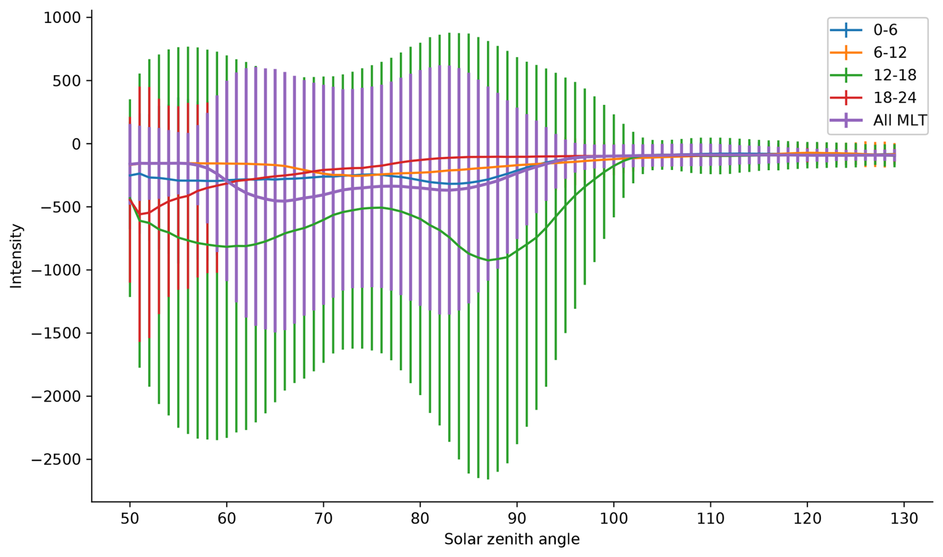
Figure 1 Mean irradiance (solid lines) and standard deviation (vertical lines) as functions of solar zenith angle (SZA), based on SSUSI measurements from regions outside the auroral oval (MLAT<60 or >80). The data are limited to periods of positive dipole tilt (April–September 2005 and 2006). No consistent trend is observed in either the mean or the variability of irradiance with increasing SZA during sunlit conditions, suggesting that solar zenith angle does not significantly influence the dayglow-residual distribution in these regions (figure taken from Hessen, 2023).

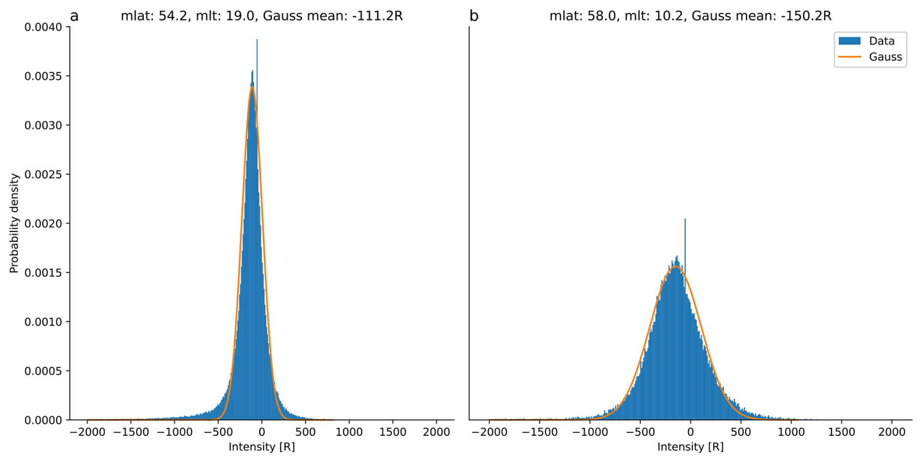
Figure 2 Normalised histograms showing typical distributions during sunlit conditions during local summer in the Northern Hemisphere with little to no aurora. A gaussian distribution is fitted to the histogram and the location parameter is extracted. These histograms are taken from the Dataset 1 (figure taken from Hessen, 2023).

Figure 3 These normalized histograms are the same as in Fig. 2, but for local winter taken from Dataset 1. The x axis is scaled to better represent the shape of the distributions (taken from Hessen, 2023).

To examine the seasons separately, we use the dipole tilt angle and select tilt >15° for local summer in the Northern Hemisphere, and tilt $<-\mathrm{15}$° for local winter in the Northern Hemisphere (opposite for the Southern Hemisphere). A description for calculating the dipole axis and dipole tilt angle can be found in Laundal and Richmond (2017).

3 Methods

3.1 Novel Method Based on Nonlinear Parameter Estimation

The data collected by the SSUSI instrument is composed of signals from the aurora and dayglow in the atmosphere. In Fig. 4 the distributions shown in each panel are the residual counts, which are the total counts minus the dayglow predicted by the Zhang et al. (2022) model. This is the default data product provided in the SSUSI files. This data product does not include measurement uncertainties; the measurements are therefore assumed to be independent and are given equal weight in all of the fits and parameter estimates presented in this study.

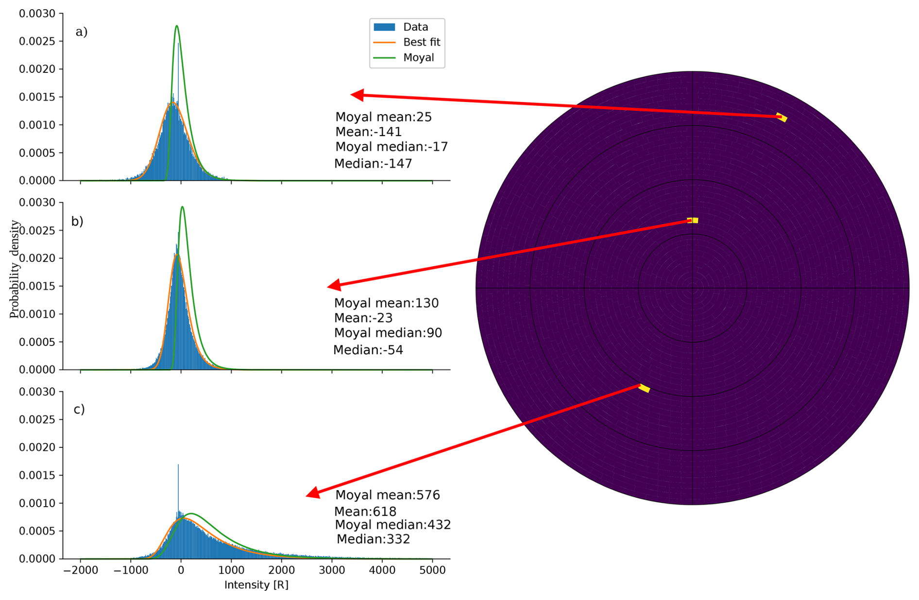
Figure 4 Residual counts in three bins showing typical residual distributions. Panel (a) shows a bin from the dayside without aurora. Panel (b) shows a bin from the dayside inside the auroral oval, and panel (c) shows a bin from the nightside in the strongest part of the auroral oval. All panels use data from Dataset 1 during local summer in the Northern Hemisphere. The curves represent the fits from the convoluted distribution labeled best fit, and the Moyal distribution plotted based on the best fitting parameters. The mean and median values are also calculated and printed in each panel (figure taken from Hessen, 2023).

The probability density function (PDF) for the Gaussian distribution is given by

$$\begin{array}{}\text{(1)}& f_{\mathrm{G}}\left(x\right)={\displaystyle \frac{\mathrm{1}}{{\mathit{\sigma }}_{\mathrm{G}}\sqrt{\mathrm{2}\mathit{\pi }}}}{e}^{-\frac{\mathrm{1}}{\mathrm{2}}{\left(\frac{x-{\mathit{\mu }}_{\mathrm{G}}}{{\mathit{\sigma }}_{\mathrm{G}}}\right)}^{\mathrm{2}}}\end{array}$$

for real values of x. Here, μ_G and and σ_G are respectively the location parameter (mean value) and scale parameter (standard deviation) of the Gaussian distribution. We use a Gaussian distribution for the dayglow (DG) residual due to its similar shape, as shown in Fig. 5a.

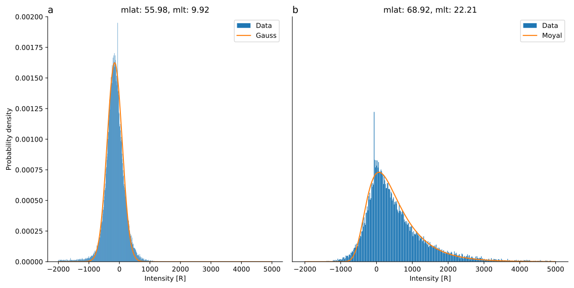
Figure 5 Normalised histograms with fitted probability distributions. Panel (a) shows a typical distribution during sunlit conditions on the dayside with little to no aurora and with a Gaussian fit. Panel (b) shows a typical distribution on the nightside with strong aurora during local summer with Moyal fit. Both panels use data from Dataset 4 (figure taken from Hessen, 2023).

The probability density function for the Moyal distribution is given by

$$\begin{array}{}\text{(2)}& f_{\mathrm{M}}\left(k\right)=e^{\frac{-\left(k+e^{-k}\right)}{\mathrm{2}}}/\sqrt{\mathrm{2}\mathit{\pi }}\end{array}$$

for real values of k. A description of the distribution can be found in Moyal (1955) and Chap. 26 in Walck (1996). We can introduce a scale parameter associated with the width of the distribution (σ_M), and a location parameter (μ_M) by making the standardized variable $k=\frac{(y-{\mathit{\mu }}_{\mathrm{M}})}{{\mathit{\sigma }}_{\mathrm{M}}}$, from which the the distribution in variable y is given by

$$\begin{array}{}\text{(3)}& g_{\mathrm{M}}\left(y\right)={\displaystyle \frac{\mathrm{1}}{{\mathit{\sigma }}_{\mathrm{M}}}}{f}_{\mathrm{M}}\left({\displaystyle \frac{y-{\mathit{\mu }}_{\mathrm{M}}}{{\mathit{\sigma }}_{\mathrm{M}}}}\right).\end{array}$$

This PDF might be useful in describing the intensity distribution of the aurora because it was invented to describe the energy loss of charged relativistic particles due to the ionization of the medium. This is similar to the process of creating aurora from energetic particles, cascading energy into secondary electrons that produce the aurora. Figure 5b shows how the Moyal distribution compares with the distribution of auroral intensities on the nightside with little to no dayglow. Such a good fit is typically seen in regions of strong aurora towards the nightside, motivating its application on describing the auroral part of the observed intensity distribution.

The distribution function in SciPy uses two parameters: location and scale. These parameters shift the distribution center and determine the width of the distribution. The Moyal distribution also has defined moments, and analytical formulas for each. We use the Moyal mean given by

$$\begin{array}{}\text{(4)}& \text{Moyal mean}={\mathit{\mu }}_{\mathrm{M}}+{\mathit{\sigma }}_{\mathrm{M}}[\mathit{\gamma }+\ln (\mathrm{2}\left)\right]\end{array}$$

where γ≈0.5772 is Euler's constant (also known as Euler Gamma) and ln (2) is the natural logarithm of 2 (Wolfram Research, 2016).

To perform the fitting, we use a Python package called LMFIT (Non-Linear Least-Squares Minimization and Curve-Fitting for Python; see Newville et al., 2014, for more information) and the convoluted probability distribution function

$$\begin{array}{}\text{(5)}& f_Z\left(z\right)=\underset{-\mathrm{\infty }}{\overset{\mathrm{\infty }}{\int }}{f}_X\left(x\right)f_Y(z-x)\mathrm{d}x,\end{array}$$

where we take $f_X\left(x\right)=f_{\mathrm{G}}(x;{\mathit{\mu }}_{\mathrm{G}},{\mathit{\sigma }}_{\mathrm{G}})$ and $f_Y\left(y\right)=g_{\mathrm{M}}(y;{\mathit{\mu }}_{\mathrm{M}},{\mathit{\sigma }}_{\mathrm{M}})$. The fitting routine then returns the parameter estimates that provide the least-squares best fit. We use these best estimates to calculate the Moyal mean (Eq. 4) and to plot the best-fit distributions of X, Y, and $Z=X+Y$ to visually verify that the fitted distribution is a good match to the observed distribution (see, e.g., Figs. 4, 6, and 7).

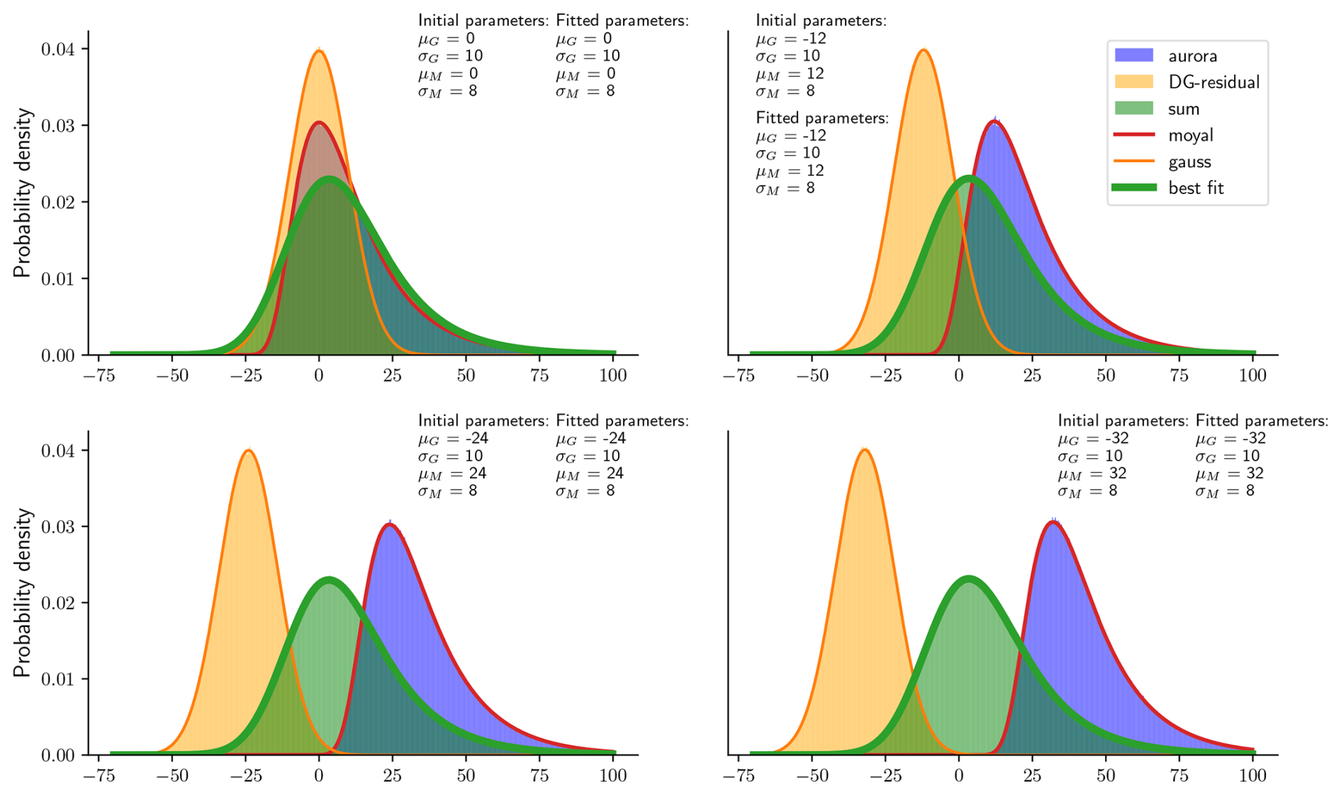
Figure 6 Randomly generated sample of normalized histograms for Moyal and Gaussian distributions. The x axis uses arbitrary units. The “Aurora” curve represents a simulated auroral intensity distribution sampled from a Moyal distribution, while the “DG-residual” curve corresponds to random values sampled from a Gaussian distribution. The “sum” curve represents the convoluted distribution given by Eq. (5). Comparison of the true and estimated parameters show that the fitting procedure accurately estimates the true parameters (figure taken from Hessen, 2023).

Figure 7 The same histograms as in Fig. 6, showing the fit and parameter extraction when the estimated center of the DG-residual deviates from its true center value (figure taken from Hessen, 2023).

3.2 Synthetic Data Example

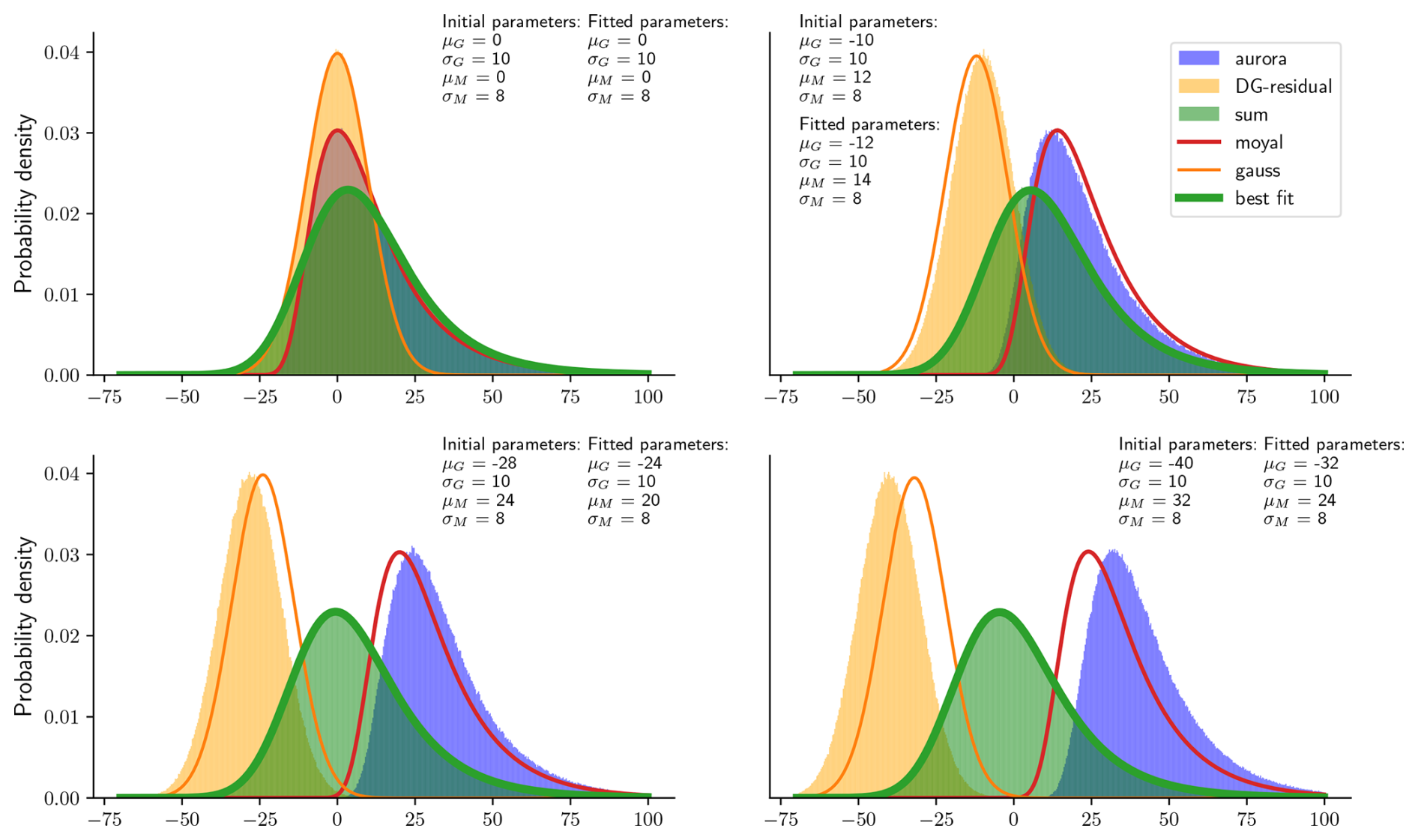
We validated the fitting procedure with randomly sampled data by generating Gaussian- and Moyal-distributed random values, summing them, and creating histograms as shown in Figs. 6 and 7.

One of the challenges posed by the convolution integral (5) is that it is not possible to estimate μ_G and μ_M separately; it is only possible to estimate the sum $\mathit{\mu }={\mathit{\mu }}_{\mathrm{M}}+{\mathit{\mu }}_{\mathrm{G}}$. This can be seen via the change of variables $v=x+{\mathit{\mu }}_{\mathrm{M}}$:

$$\begin{array}{rl}{f}_Z\left(z\right)& =\underset{-\mathrm{\infty }}{\overset{\mathrm{\infty }}{\int }}{f}_X(x-{\mathit{\mu }}_{\mathrm{G}})f_Y(z-x-{\mathit{\mu }}_{\mathrm{M}})\mathrm{d}x\\ & =\underset{-\mathrm{\infty }}{\overset{\mathrm{\infty }}{\int }}{f}_X(v-({\mathit{\mu }}_{\mathrm{G}}+{\mathit{\mu }}_{\mathrm{M}}\left)\right)f_Y(z-v)\mathrm{d}v.\end{array}$$

First, we attempted to simultaneously estimate all four parameters (μ_M, σ_M, μ_G, and σ_G). However, this turns out to not be a uniquely defined problem. This is because several different values of μ_G and μ_M yield the same result. The convoluted distribution may appear similar for different locations of the underlying distributions. Hence, the convoluted PDF is not suitable for constraining the locations of both the DG-residual and aurora, and we must assume one of the locations is known. It makes sense to fix μ_G because it is easier to estimate from the data in regions outside the auroral oval than to estimate the location parameter of the auroral part of the signal. With μ_G fixed we can estimate the three remaining parameters (μ_M,σ_M and σ_G).

Figures 6 and 7 show results of the fits (solid lines). The fit and parameter extraction in Fig. 6 is successful when using the known μ_G. Here, the correct μ_M, σ_M and σ_G are extracted. The location of the plotted Gaussian distribution is taken from the input values to show the result of the fit.

Since we do not know the exact value that μ_G should have, it represents a source of uncertainty. Figure 7 illustrates with synthetic data how the extracted parameters related to the Moyal distribution differ from the actual distribution parameters when the assumed μ_G differs from the true location. This must be taken into consideration when interpreting the modeled intensities from our separation method. From Fig. 7 we can see that the error in the estimated value of μ_G (its deviation from the true value) and the corresponding error in the fitted μ_M is such that their sum is preserved.

Equation (4) shows how the Moyal mean is calculated. The fitting function returns the correct values of σ_G and σ_M in all cases; only the estimated value of μ_M is affected by our choice of μ_G. Consequently, the error in the DG-residual estimate causes an equal error in the Moyal mean estimate, as discussed above. From manual examination of individual fits we find that typical fit parameter uncertainties are 0.5 %–2 %.

When applying the separation method to the data, we interpret the Moyal mean as a proxy for auroral intensity. From this, we can apply the method to real data from the SSUSI auroral dataset.

3.3 Application of the Method on SSUSI Data

To apply the method to the data, we first collect the data in bins based on the grid, and create histograms, as shown in Fig. 5. The histograms are limited in intensity from −2000–5000 R to save on computation time. Truncating the window like this does not significantly affect estimation of either the mean or Moyal mean. The estimates are saved for each bin, and plotted as a polar plot.

3.4 Real Data Example

In Fig. 4a shows the performance of the fit on a bin with little to no aurora. As expected, the Moyal mean estimates a larger value than the regular mean. This is also the case in panel (b), where we have more aurora than in panel (a), but it is still sunlit, being on the dayside during local summer. In panel (c) the regular mean estimates a value larger than the Moyal mean, and this is because of the long tail in this bin that the Moyal distributions does not capture. As can be seen in these panels, the convoluted distribution fits well to the real data in these bins. Therefore we argue that this method is a fair representation of statistical auroral intensities.

3.5 Estimating Auroral Boundaries

We use the Ohma et al. (2023) method to estimate auroral boundaries. The code can be found at https://github.com/aohma/fuvpy (last access: 18 October 2023). The boundary method is a two-step process. First, the initial boundaries are identified by dividing the plot into slices and then estimating the threshold of the aurora in that slice. The model is then fitted to the initial boundaries found in the slices. This model is based on a Fourier series and uses three terms for equatorward boundaries and six terms for poleward boundaries. We have made minor alterations to fit our use, such as not considering the temporal evolution of the boundaries, as we look at statistics. We also modified the detection range for auroral boundaries to match the variations in our statistical maps, while visually being the best fit. During local summer, these threshold values are: 300–450 R in 5 R increments. During local winter, they are: 170–250 R in 5 R increments. To give an indication of the level of variation, or spread, of the estimated boundaries, we plot each set of boundary estimates individually. The boundary estimation method uses regularization to be even in the east-west direction unless the data suggests otherwise. Thus, there is little variation in the areas without data, primarily on the nightside below ∼72° MLat where there are few or no measurements.

3.6 Modeling Ionospheric Convection

We utilized the Swarm Ionospheric Polar Electrodynamics (Swipe) empirical model to represent high-latitude ionospheric electrodynamics (Hatch, 2023). The SWIPE model is parameterized by the interplanetary magnetic field (IMF) components B_z and B_y, solar wind velocity V_x, dipole tilt angle, and the solar flux index in the F10.7 cm band, and provides electric field maps for both hemispheres based on the specified input parameters. The model is constructed using data collected by the Swarm and Challenging Mini-satellite Payload (CHAMP) satellites, and was developed to closely mirror the Swarm-based Average Magnetic field and Polar current System (AMPS) model, which characterizes large-scale ionospheric currents. For further details on the Swarm mission and its instrumentation, see Knudsen et al. (2017). The source code is available at https://doi.org/10.5281/zenodo.10148940, Hatch, 2023). In our implementation, we modified several functions within the code to generate maps of the same hemisphere under varying IMF B_y conditions.

4 Results

4.1 Northern Hemisphere

Figure 8 shows our results for the Northern Hemisphere during local summer (dipole tilt angle >15°) and IMF B_y>5 nT. The Moyal mean and the total mean are respectively shown in the left and middle column. To facilitate comparison of the two means, the difference between the two is shown in the column at right. The number on the label for each row indicates the dataset represented by the row. In the difference plots, we can see that our method is usually around 100–150 R brighter than the total mean, with the difference being smaller in areas with stronger aurora. The boundary model detects different boundaries for the total mean and the Moyal mean. For example, the boundary is narrower for the total mean, particularly in the dayside area of the oval. The typical latitudinal range of both the equatorward and poleward boundaries generally agree well with auroral boundaries identified in other recent studies (Decotte et al., 2023; Walker et al., 2024).

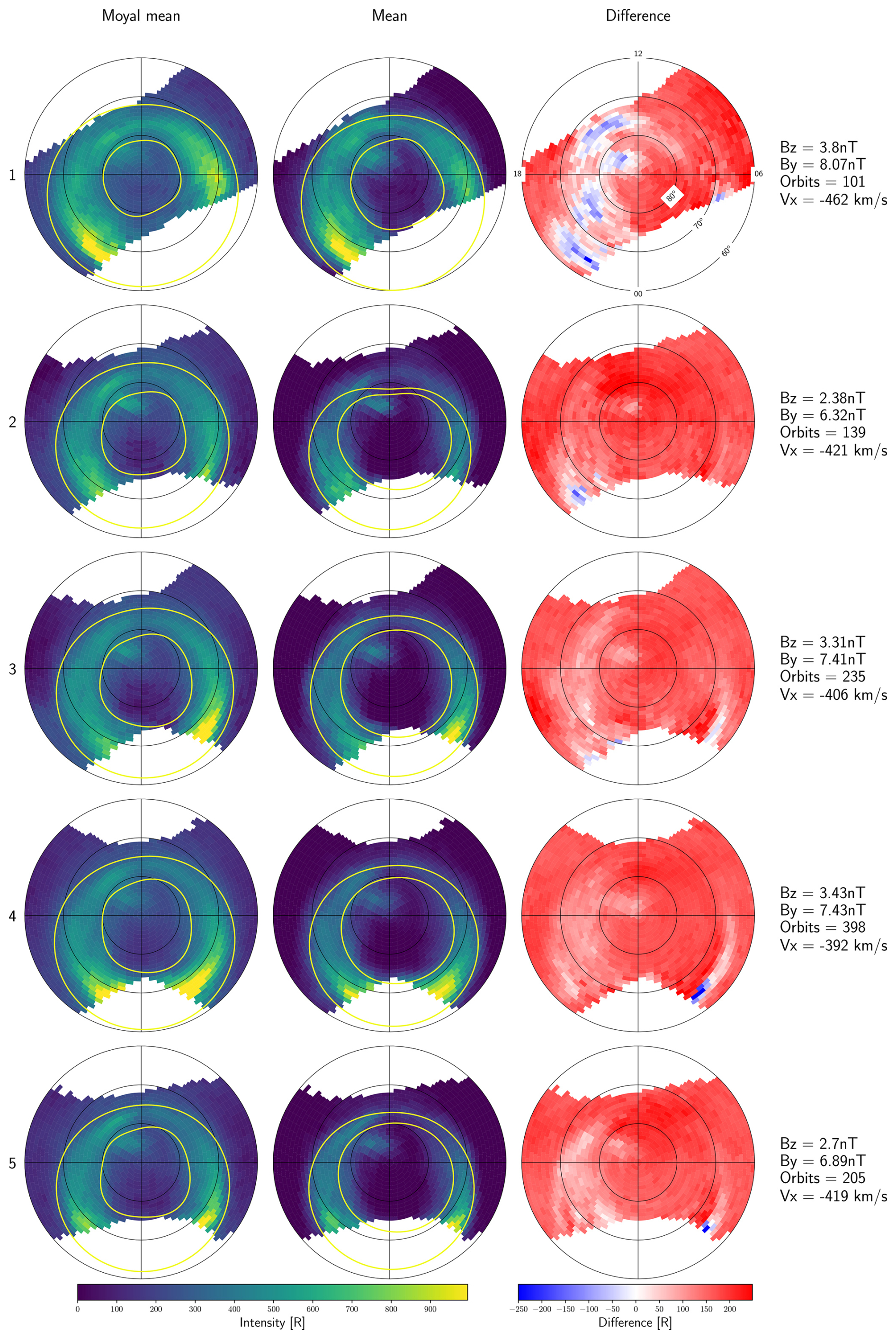
Figure 8 Northern Hemisphere maps of the Moyal mean (left), regular mean (center), and the difference between them (right) for IMF B_y>5 nT and dipole tilt angle >15° (local summer). The rows are numbered according to the dataset from which they are produced. The text box at right in each row indicates mean solar wind conditions and the number of orbits. Yellow lines indicate the auroral zone boundaries obtained via the method described in Sect. 3.5.

In all the rows, the total mean estimates of the oval extent are much smaller around the pre- and post-noon sectors at approximately 80° MLAT. This can be seen in the estimated boundaries, as this sector has a much narrower band than the boundaries estimated by the Moyal mean. Generally, for these rows, the polar cap estimated by the Moyal mean is smaller than that estimated by the total mean.

The bright spot located in the polar cap between 11 and 15 MLT is called the high-latitude dayside aurora (HiLDA). This spot is visible in statistics for both methods of calculating the mean. More detailed descriptions of HiLDA can be found elsewhere (Frey, 2003; Frey et al., 2004; Frey, 2007; Carter et al., 2018).

Figure 9 is the same as Fig. 8, but the data selected is for IMF $B_y<-\mathrm{5}$ nT. We observe mostly the same patterns in the difference plots. The boundaries in the total mean plots seem very narrow on the dayside compared to the Moyal mean boundaries. There appear to be considerable differences inside the polar cap, and the Moyal mean estimates are much higher (∼100–250 R) than the total mean.

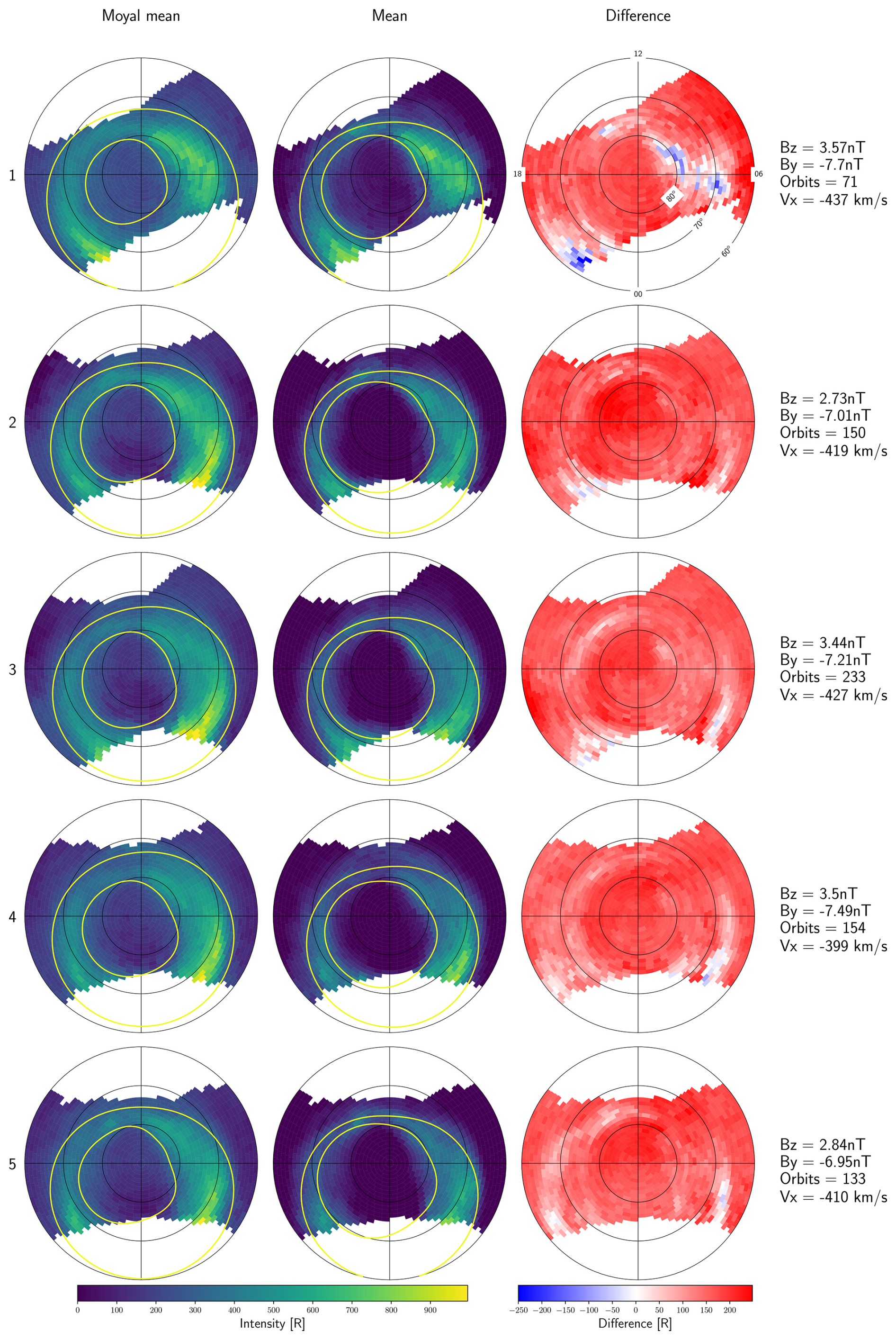
Figure 9 Northern Hemisphere maps of the Moyal and regular means as well as the difference between them for IMF $B_y<-\mathrm{5}$ nT and dipole tilt angle >15° (local summer), in the same layout as Fig. 8.

A dawn-dusk shift appears in the polar cap location in Figs. 8 and 9. In particular the dusk sector in Fig. 8 appears wider and stronger than in Fig. 9, while the dawn sector in Fig. 9 appears wider and stronger than in Fig. 8. Both of these features can be seen in boundaries derived from both the Moyal mean and regular mean statistics. The sign of IMF B_y does not appear to affect the overall intensities in the auroral oval.

Figure 10 (Fig. 11) shows the Moyal mean, total mean, and the difference between them for dipole tilt angle $<-\mathrm{15}$° and IMF B_y>5 nT (IMF $B_y<-\mathrm{5}$ nT). The data selection represents local winter conditions in the Northern Hemisphere.

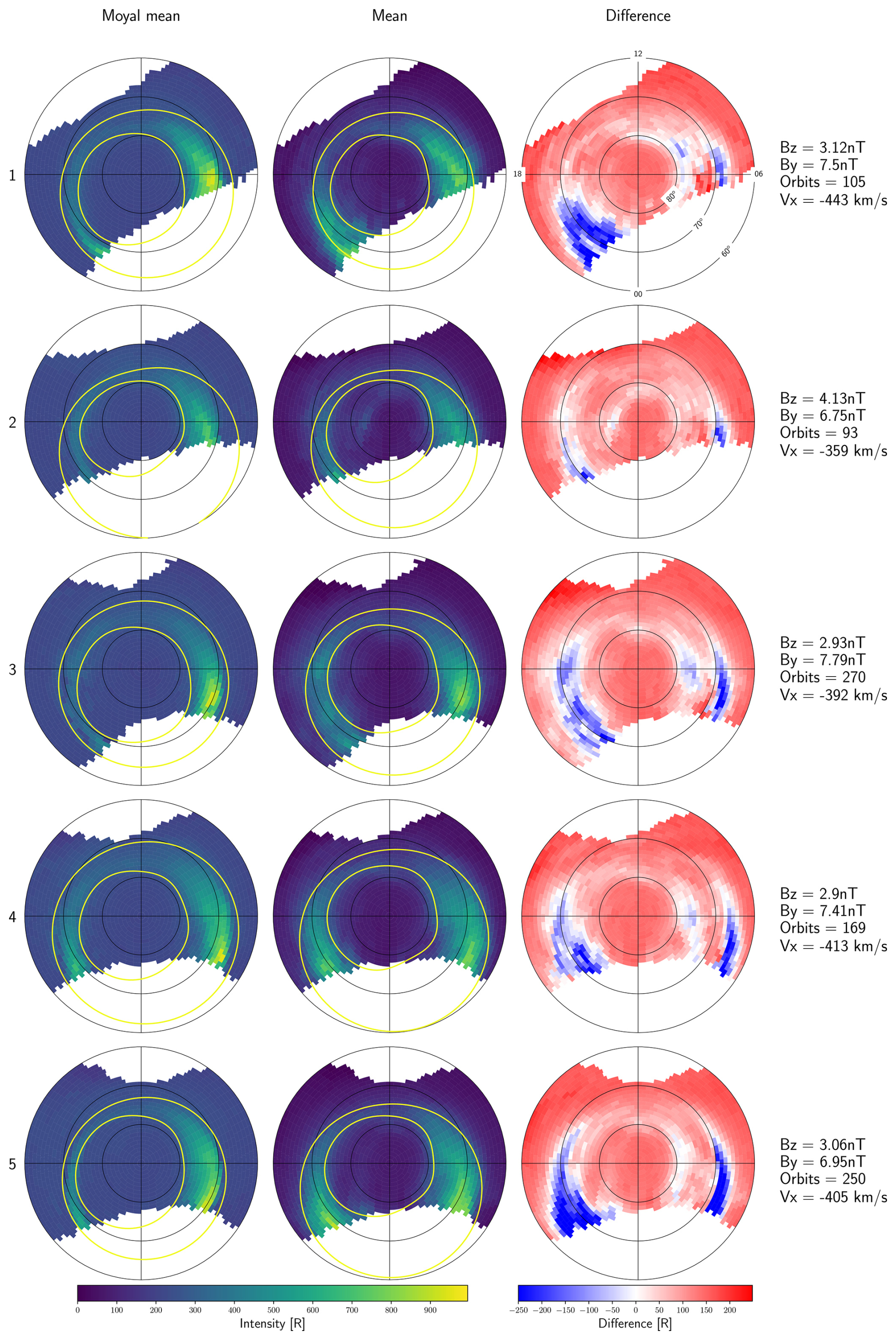
Figure 10 Northern Hemisphere mean statistics and their difference for IMF $B_y<-\mathrm{5}$ nT and dipole tilt angle $<-\mathrm{15}$° (local winter), in the same layout as Fig. 8.

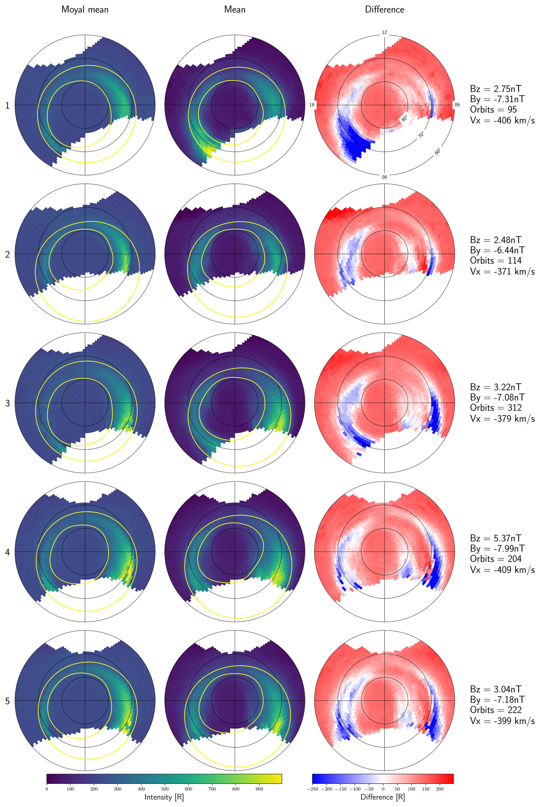
Figure 11 Northern Hemisphere mean statistics and their difference for IMF $B_y<-\mathrm{5}$ nT and dipole tilt angle $<-\mathrm{15}$° (local winter), in the same layout as Fig. 8.

In Fig. 10 the Moyal mean-based estimates of auroral intensity is overall larger than the mean-based estimates outside the oval, as well as in the part of the oval in the noon sector. In the night side of the oval, which is completely dark, the total mean-based estimates are much larger than the Moyal mean-based estimates. In the area around noon, the Moyal mean tends to estimate slightly wider boundaries, whereas in the pre- and post-midnight sectors, the total mean estimates lead to wider boundaries than those associated with the Moyal mean. All the rows seem to follow similar patterns, with stronger intensity and wider auroral oval on the dawn side.

In Fig. 11 the differences between Moyal mean-based statistics and those based on the total mean are approximately the same as in Fig. 10. The intensities and boundaries follow similar patterns, with the Moyal mean-based estimates of auroral intensity within the oval (except for the noon sector) overall lower than those based on the total mean. The spot found in the polar cap in the second row of Fig. 10 does not appear in the second row of this plot.

The mirror asymmetry in the dawn-dusk shift of the polar cap location and difference in intensities between dawn and dusk found in Figs. 8 and 9 is not evident in these plots. The polar cap appears to be in the same place and the dawn sector appears to be the widest and strongest for both signs of IMF B_y. During negative IMF B_y, the polar cap appears to be elongated compared with a more circular polar cap during positive IMF B_y. As in the summer case, the sign of IMF B_y does not appear to affect the auroral intensities overall in the auroral oval.

4.2 Southern Hemisphere

Because of the inclination of the Sun synchronous orbit of the DMSP (Defense Meteorological Satellite Program) satellites, the coverage of the SSUSI instrument is more towards the nightside in the Southern Hemisphere, especially during local summer (tilt $<-\mathrm{15}$°). However, we can still perform the boundary-estimation and carry out a limited comparison with the Northern Hemisphere.

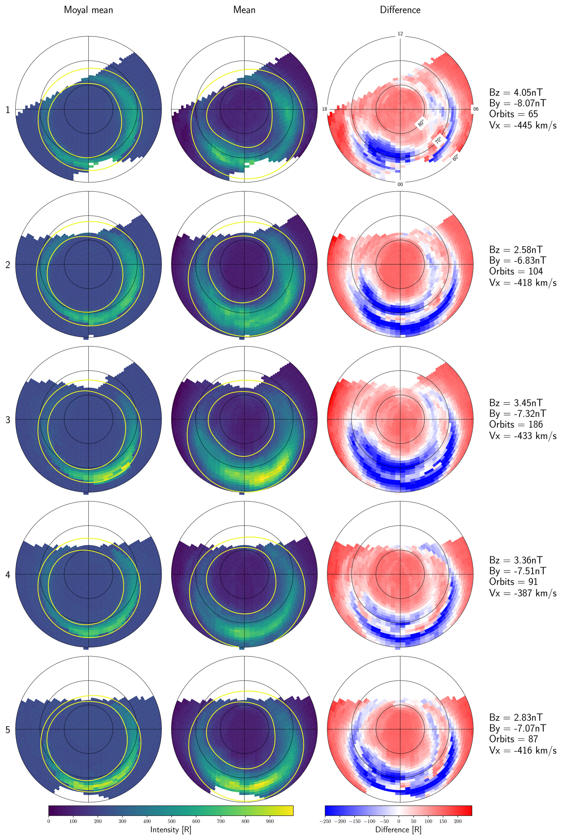
Figures 12 and 13 show that in the Southern Hemisphere, DMSP coverage is almost exclusively confined to the nightside, and coverage of the dayside is extremely limited. Despite the poor coverage on the dayside, the summer plots suggest that there is a shift in the polar cap location with a dependence on IMF B_y that is opposite the dependence observed for the Northern Hemisphere. This is most clearly observed in Datasets 3–5. The dawn sector appears to be brighter and wider during positive IMF B_y, whereas the dusk sector appears to be brighter and wider for negative IMF B_y. This sign dependence is likewise opposite the dependence observed for the Northern Hemisphere.

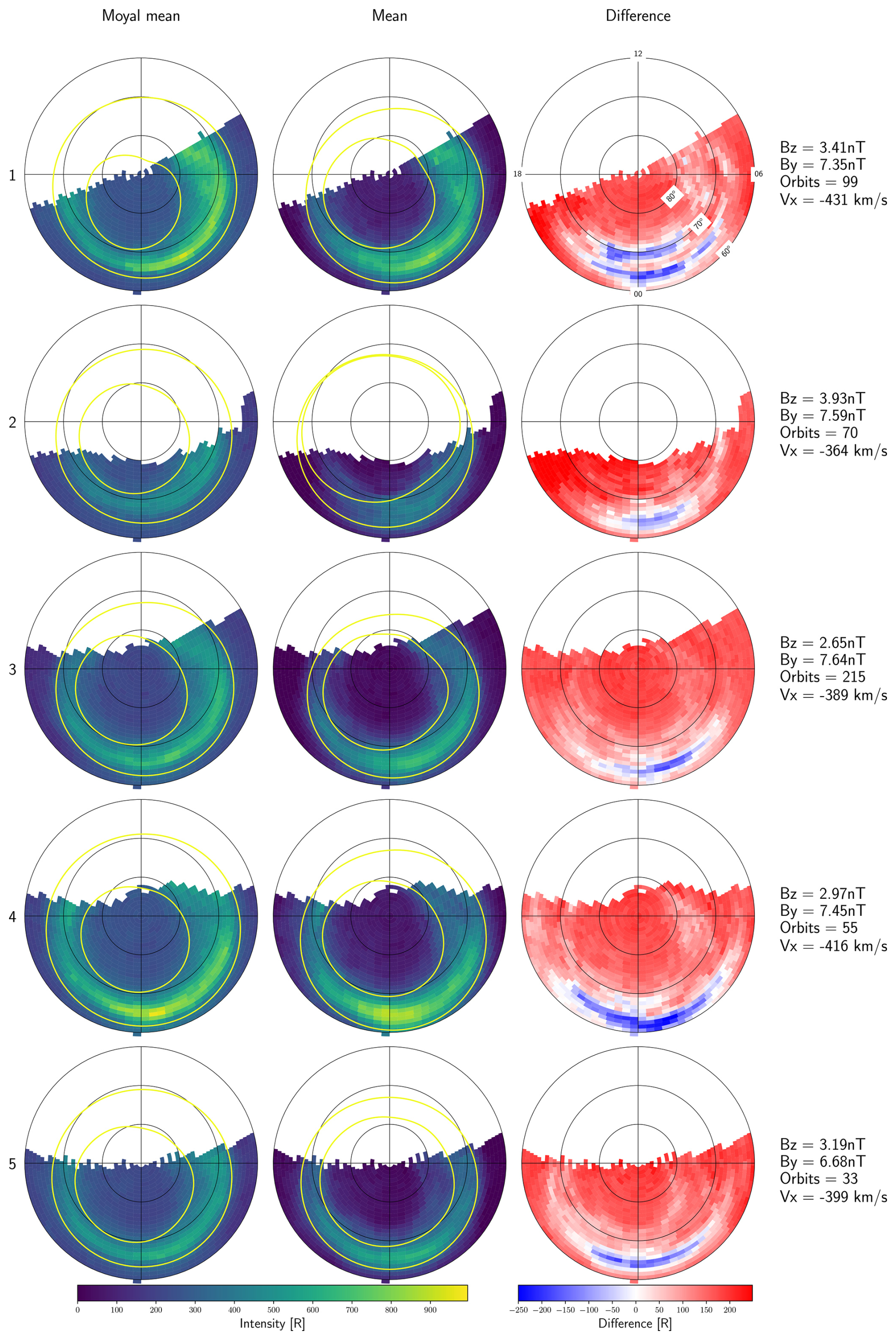
Figure 12 Southern Hemisphere auroral intensity statistics for dipole tilt $<-\mathrm{15}$° (local summer) and IMF B_y>5 nT in the same format as Fig. 8.

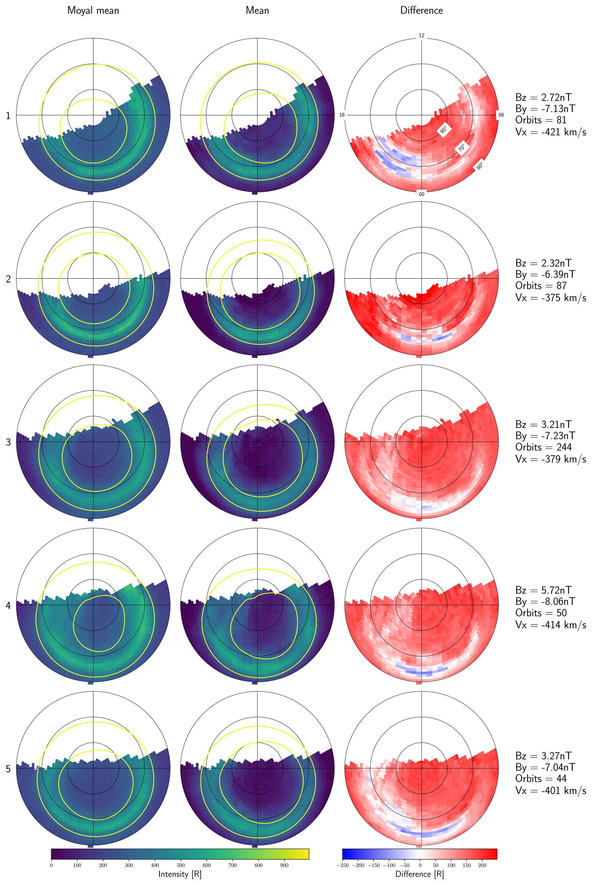
Figure 13 Southern Hemisphere auroral intensity statistics for dipole tilt $<-\mathrm{15}$° (local summer) and IMF $B_y<-\mathrm{5}$ nT in the same layout as Fig. 8.

In Figs. 14 and 15 we see that we have good data coverage during local winter in the Southern Hemisphere and that the boundaries derived from the Moyal mean are significantly narrower than the boundaries derived from total mean statistics. This is similar to the results obtained for local winter in the Northern Hemisphere (Figs. 10 and 11). As in the Northern Hemisphere, the IMF B_y dependent shift in polar cap location is absent during local winter. In these figures, it appears that the auroral oval is the widest and strongest in the post-midnight sector for both IMF B_y polarities, which is consistent with the Northern Hemisphere. The intensities are also similar for ± IMF B_y when looking at the same dataset, except for the midnight sector in Dataset 3. The systematic IMF B_y-dependent deformation of the polar cap during local winter is also present in the Southern Hemisphere.

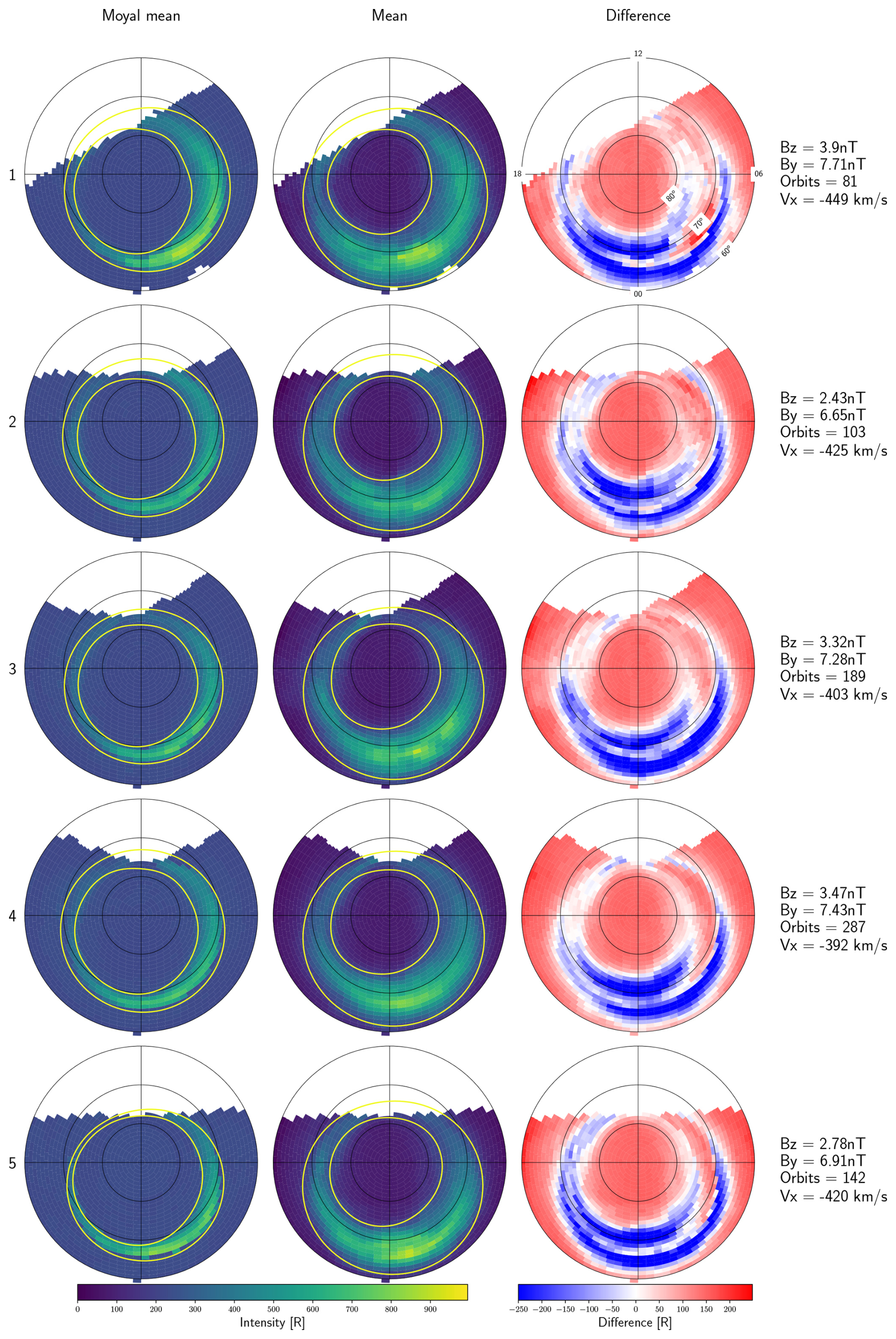
Figure 14 Southern Hemisphere statistics of auroral intensity for IMF B_y>5 nT and dipole tilt angle >15° (local winter), in the same layout as Fig. 8.

Figure 15 Southern Hemisphere auroral intensity statistics for IMF $B_y<-\mathrm{5}$ nT and dipole tilt angle >15° (local winter), in the same layout as Fig. 8.

4.3 The Shift in Polar Cap Location

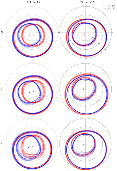
Figures 16 and 17 show the seasonal dependence of the shift in the polar cap found in our results for the Northern and Southern Hemispheres respectively. Previous studies mention an IMF B_y-dependent displacement in the boundaries and center of the polar cap (Meng, 1979; Cowley et al., 1991; Rich and Hairston, 1994). However, these studies did not consider seasonal effects. For negative IMF B_y the polar cap is displaced towards dusk, and for positive IMF B_y the polar cap is displaced towards dawn during local summer in the Northern Hemisphere (opposite polarity for the Southern Hemisphere).

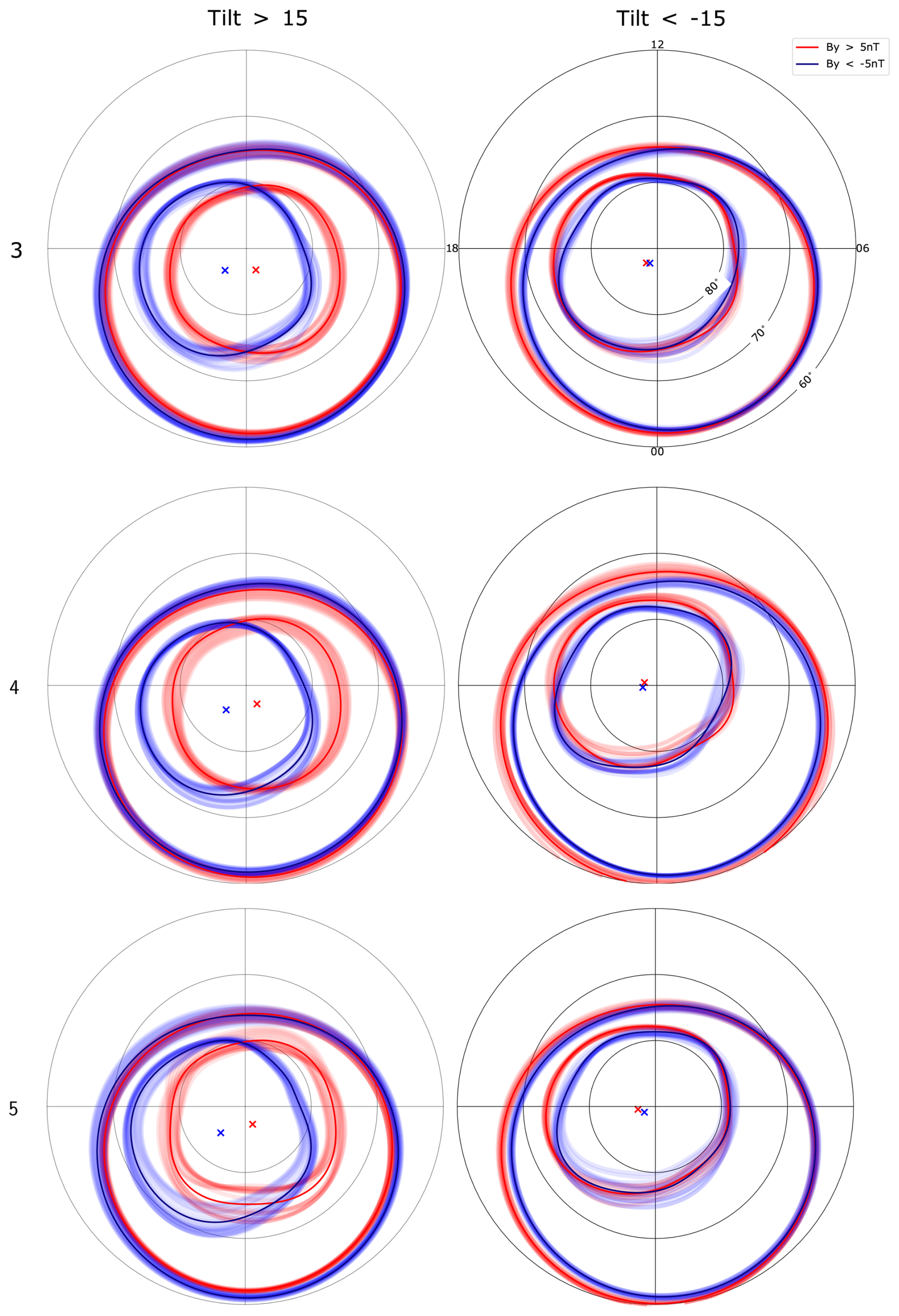
Figure 16 Northern Hemisphere auroral boundaries obtained from Datasets 3–5 during local summer (left) and local winter (right). Each panel contains results for both positive and negative IMF B_y (shown in red and blue, respectively). Local summer boundaries are based on the Moyal mean, while local winter boundaries are based on the total mean. The crosses represent the estimated center values for the ovals.

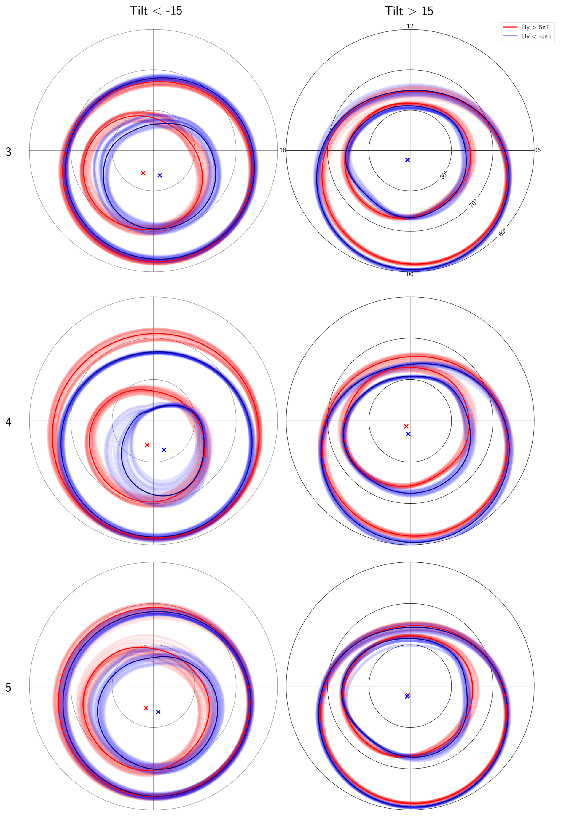
Figure 17 Southern Hemisphere auroral boundaries in the same layout as Fig. 16, with boundaries for local summer derived from Moyal mean statistics and those for local winter derived from total mean statistics.

The center of the polar caps was determined using the Haversine formula at a mean emission height of 130 km above the Earth's surface (shown as crosses in Figs. 16 and 17). The formula was first used to determine the distance between each MLT step in the estimated boundaries. The center was then calculated using the weighted average of all the points in the estimated boundaries, using the previously calculated distance between MLT–steps as weights. Using the center values obtained from Datasets 1 to 5, we found a mean distance of 492 km with a standard deviation of 16 km between the centers of the polar caps for positive IMF B_y and negative IMF B_y in the Northern Hemisphere. The corresponding numbers for the Southern Hemisphere using Datasets 3–5 is a mean displacement of 430 km with a standard deviation of 50 km. The larger standard deviation in the Southern Hemisphere is caused by the displacement in Dataset 5, which is 100 km smaller than for Datasets 3 and 4.

During local winter in the both hemispheres, there is no significant systematic shift in the center of the polar caps. For negative IMF B_y, the polar cap boundaries in the Northern Hemisphere appear to take on an elongated shape, whereas the polar cap boundaries remain mostly circular for positive IMF B_y. The cause of this elongation will not be further explored in this study.

During local summer in the Northern Hemisphere, there is a clear difference in the width and intensity of the dawn and dusk sectors of the auroral oval depending on the sign of IMF B_y. For positive IMF B_y, the dusk sector of the auroral oval is wider and brighter than the dawn sector. This is opposite for negative IMF B_y. This may simply be related to the shift in polar cap location, making the auroral oval wider in the section opposite of the shift direction, as the equatorward boundaries remain largely unaffected by the sign of IMF B_y. These effects are also present in the Southern Hemisphere, but with the sign of IMF B_y reversed.

5 Discussion

In this study, we introduced a novel method of further refining the auroral signal for statistical analysis of SSUSI EDR data. Then the method was applied to a large amount of data during northward IMF with a significant IMF B_y-component, and compared between the seasons approximated by the dipole tilt angle. Here we discuss the efficacy of the method, as well as describe possible physical mechanisms behind the observed shift in polar cap location. These mechanisms are closely tied to the circulation of plasma and magnetic fields, and therefore we also describe how the convection pattern changes, using an empirical model.

5.1 Assessing the Validity and Performance of the Separation Method

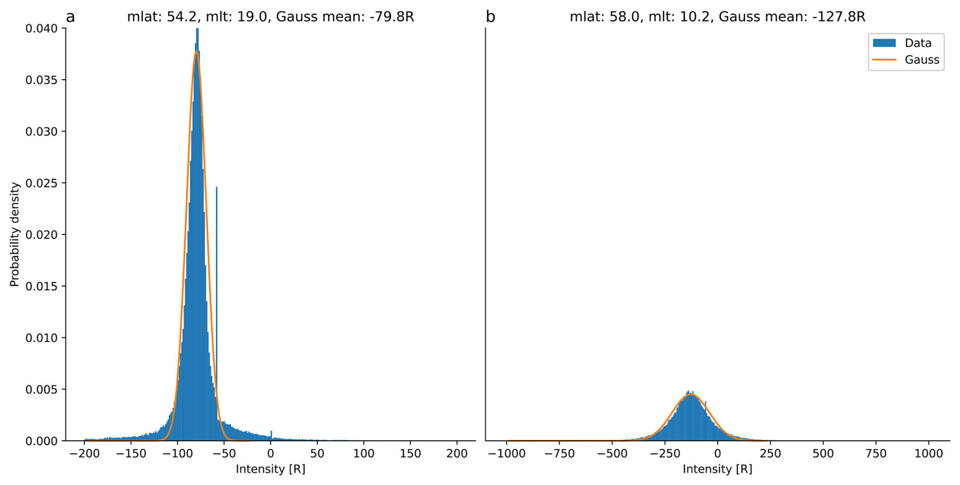
The choice of distribution can significantly influence estimation of auroral intensity . Selecting a different distribution with a shape similar to the Moyal distribution would yield different modeled mean values. We chose the Moyal distribution because it performs well under sunlit conditions and for aurora with little to no dayglow during local summer. However, as shown in Fig. 18, the Moyal distribution often yields a poorer fit to the data for distributions from local winter. It only succeeds in certain cases, such as in the post-midnight sector during strong auroral activity during local winter (panel (b)). A likely explanation for these failures is that the assumption $Z=X+Y$ where X and Y are Gaussian and Moyal distributed, respectively, is an oversimplification. In reality, auroral intensity at any given location within the auroral oval varies depending on, for example, the level of geomagnetic activity. In terms of distributions, it may be more conceptually appropriate to think of the distribution of auroral intensities Y itself as a combination of several Moyal distributions having different means and spreads. Implementing this would be a significant effort that is outside the scope of the present study.

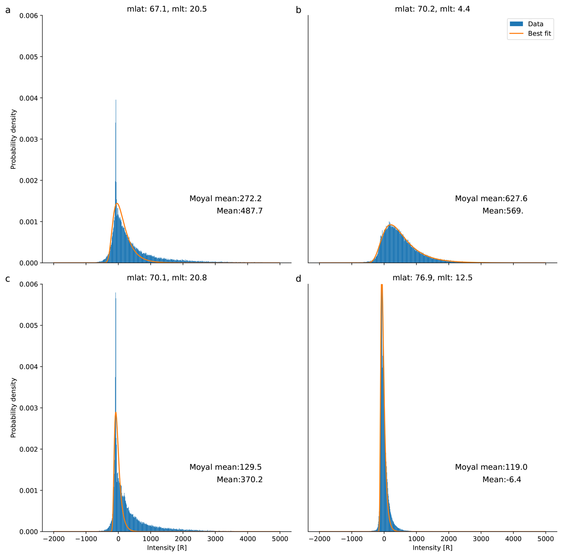
Figure 18 Normalized histograms illustrating typical distributions observed during local winter within the auroral oval in the Northern Hemisphere. Panels (a), (b), and (c) correspond to bins from the nightside, while panel (d) represents a bin from the dayside. The data is sourced from Dataset 4, with a dipole tilt angle of $<-\mathrm{15}$° (figure taken from Hessen, 2023).

In certain areas, the fit performs poorly due to the shape of the data distribution. Figure 18 shows normalized histograms of data from four bins in the auroral oval during local winter in the Northern Hemisphere. In panels (a) and (c), the fitted Moyal distribution falls off too quickly, failing to capture the tails of the data. Conversely, in panel (b), the data closely follows the shape of a pure Moyal distribution. Panels (b) and (c) represent bins at the same MLAT but approximately 4 h MLT apart (on either side of midnight), yet they exhibit very different distributions.

A trend emerges in the post-midnight auroral oval around 70° MLAT during local winter, where the distribution of intensities often takes on a Moyal-like shape. Pre-midnight, however, the data tends to exhibit a steeper distribution, as seen in panels (a) and (c). Additionally, spikes are present in panels (a) and (c), typically between −100 and 0 R, which adversely affect the fit. These spikes may cause the fitting function to overemphasize narrow features, resulting in fits that are too narrow overall. This challenge is one reason why we rely on the total mean to estimate boundaries during local winter. The failure of the fitting function is evident in the blue regions of the difference plots in Figs. 10 and 11. This approach is reasonable, as significant dayglow is not expected in these regions during local winter, and our method was originally designed to isolate the auroral signal from a dayglow residual. However, the cause of the negative tails in the distributions remains unclear. In panel (d), the distribution is narrow with a spike in the same range as observed during local summer (−50 to −60 R). While this spike is not visible due to the range of the histogram's y axis, it suggests the presence of some dayglow, which is plausible given the bin's location. The fit is nevertheless a relatively poor representation of the intensity distribution. We therefore deem the total mean to yield a more appropriate measure of aurora during local winter.

Figure 19 shows the distributions for the same bins as in Fig. 18, but during local summer in the Northern Hemisphere. Here, the distributions are dominated by a symmetrical component near the center, which corresponds to the DG-residual. Under these conditions, the fit error is significantly lower. However, in panel (d), a small but notable leftward tail introduces a discrepancy, causing the total mean to take on a more negative value than is likely realistic. The origin of this left tail is unknown, however it may be related to the counting errors left from the dayglow-removal routine. The tail is relatively flat and extends into very negative values. During local summer, a spike is also consistently present in the range of −50 to −60 R across nearly all bins. Unlike during winter, this spike is narrow and does not significantly affect the fit.

Figure 19 Normalized histograms similar to those in Fig. 18, but for local summer conditions in the auroral oval in the Northern Hemisphere. The data is taken from Dataset 4, with a dipole tilt angle of >15° (figure taken from Hessen, 2023).

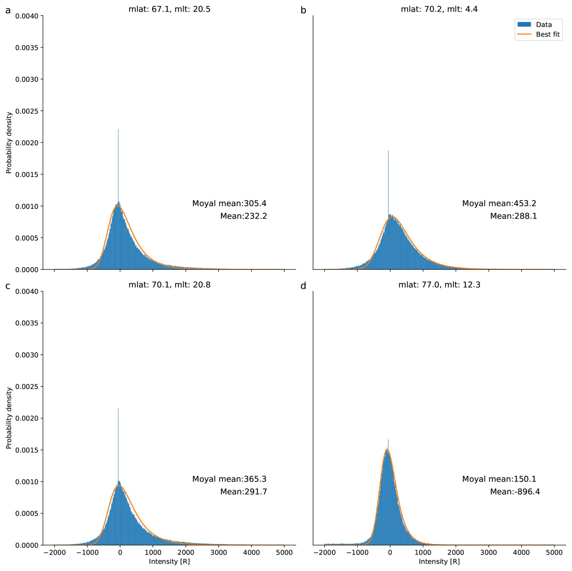
One of the primary sources of uncertainty in our method stems from the SSUSI EDR Auroral dataset and the Scanning Imaging Spectrograph (SIS) instrument. The dayglow-removal model often overestimates the subtraction, resulting in a dataset with a negative bias. The negative values are caused by data processing: removing scatters from bright emissions (H121.6 nm, O130.4 nm and O135.6 nm) into the LBH bands and counting errors. The isolated spikes are due to glints and MeV particle noise. Ideally, the dayglow residual (DG-residual) should be centered around 0 R, but this is rarely the case. The value of ${\mathit{\mu }}_{\mathrm{G}}=-\mathrm{150}$ R that we assume for local summer is only an average value and varies slightly across the MLT/MLAT grid.

To improve the precision of estimates of average auroral intensity a more precise model of this offset is needed, assigning a unique offset to each bin prior to fitting since our fitting procedure cannot simultaneously determine both location parameters (see Sect. 3.1). Within the auroral zone, the presence of aurora makes it difficult to determine offsets. Because of this, assumptions based on bins located north and south of the auroral zone were used in the fitting in the auroral zone. Figures 6 and 7 in Sect. 3.2 highlight how DG-residual locations influence the extracted Moyal parameters and modeled intensities. Given these dataset-related challenges, differences of ≲100 R across the MLT/MLAT grid should be viewed as noise. However, variations over smaller regions, such as within the auroral oval, are less impacted by this negative baseline issue.

During local summer, small regions on the nightside exhibit total mean estimates that exceed the Moyal mean, as shown in the figures in Sect. 4.1 and 4.2. This discrepancy may result from a combination of reduced sunlight on the nightside and stronger auroral activity due to magnetotail reconnection. It is likely that the distribution deviates from the one assumed in the convolution, which leads to suboptimal fits as seen in the winter example in Fig. 18 where the Moyal distribution declines too rapidly relative to the observed intensity distribution. During summer, this issue is fortunately confined to a few small areas, and the Moyal mean appears to constitute an overall good estimate of the average auroral intensity.

In the Northern Hemisphere’s local winter, our method tends to underestimate auroral intensities compared to the total mean across much of the auroral oval, as shown in panels (a) and (c) of Fig. 18. However, in the dayside region (typically between 10–14 MLT and 70–80° MLAT), our method estimates stronger auroral intensities than the total mean. This is likely due to sufficient solar illumination in this region during local winter, which affects the total mean through DG-residuals. Despite this, the fit is not perfect, as the fitted distribution declines too rapidly (see panels (a) and (c) of Fig. 18). For this reason, we rely on the boundaries and values provided by the total mean during local winter.

In the polar cap, our method also returns higher values than the total mean. This may occur because our method avoids producing negative values in areas without aurora, unlike the total mean, which can include negative tails. Panel (d) of Fig. 19 demonstrates how negative tails in the distribution are avoided during fitting, even though this example pertains to local summer. This issue is particularly prevalent on the dayside during summer for Datasets 3–5. By concentrating on the main shape of the distribution, our method avoids these negative counts.

The nonlinear fitting software (LMFIT) returns the uncertainties of the fitted parameters. These are usually less than 10 % with successful fits during the local summer, with the vast majority of the fits returning uncertainties of 0.5 %–2 %. The main source of uncertainty during summer appears to be the observation that could be considered faulty, based on the large negative counts in certain bins, and the prescribed shape of the distributions we have chosen, as discussed above.

5.2 Potential Cause of the Displacement of the Polar Caps

During reconnection between the IMF and the magnetosphere with a significant IMF B_y component, forces and stresses in the dawn/dusk directions are applied to the Earth's magnetic field. Figure 2 in Cowley et al. (1991) shows how the IMF B_y component changes the position of the geomagnetic field lines, as viewed from the Sun. In Cowley et al. (1991) the authors suggested that the displacements observed in the geomagnetic field lines can be explained by a “dipole plus uniform magnetic field” model. In the Northern Hemisphere, the field lines lying in the dawn-dusk meridian experience a shift in the direction opposite to that of the added magnetic field.

According to Holzworth and Meng (1975), the aurora mainly occurs at the boundaries of open and closed flux, as shown in Fig. 1 in Milan et al. (2012). Thus, forces that change the location of the boundaries also affect the location of the aurora.

During northward IMF, reconnection occurs on lobe field lines poleward of the cusp (Dungey, 1963; Watanabe et al., 2005; Dorelli et al., 2007). During single-lobe reconnection, the IMF reconnects with lobe field lines in one hemisphere. This occurs when a significant IMF B_y component exists (Milan et al., 2022). These opened field lines drape over the dayside (Crooker, 1992). Figure 19 in Maezawa (1976) shows lobe reconnection with northward IMF and the draping across the dayside magnetopause. When an IMF B_y component is introduced, Crooker and Rich (1993) suggest that the draped field line may drift duskward for IMF B_y<0 or dawnward for IMF B_y>0. This is due to a kink in the field line after reconnection, pointing in the opposite direction of the IMF B_y, which causes a tension force that moves the field line in the direction opposite to IMF B_y (Milan et al., 2022).

In the Northern Hemisphere for positive IMF B_y, the polar cap is shifted towards dawn, whereas for negative IMF B_y it is shifted towards dusk (opposite in the Southern Hemisphere). Figure 16 shows that the location of the polar cap varies substantially more (∼500 km) for positive dipole tilt than for negative dipole tilt in the Northern Hemisphere. To our knowledge, this dipole tilt dependence of the dawn-dusk shift of the polar cap has not been reported previously.

Lobe reconnection appears to be the most likely explanation for the seasonally dependent dawn-dusk shift in polar cap location. This is because lobe reconnection becomes more efficient in the hemisphere that is tilted towards the Sun (Wilder et al., 2010; Pettigrew et al., 2010; Crooker and Rich, 1993; Reistad et al., 2021). The fact that this polar cap shift is seen in both hemispheres for the opposite sign of IMF B_y strengthens our hypothesis that this is due to lobe reconnection. The seasonal and IMF B_y polarity-dependent widening and brightening of the dawn/dusk sector of the auroral oval might also be related to the seasonal change in lobe reconnection efficiency. This shift in polar cap location may be interpreted as a direct influence of the IMF forcing on open field lines. The striking differences between local summer and local winter may therefore relate to the vastly different forcing from the IMF on the open field lines. This effect is likely exaggerated during northward IMF as little tail reconnection takes place, allowing the magnetosphere to retain a highly asymmetric shape (Ohma et al., 2019, 2021).

5.3 Relation to Ionospheric Convection

Magnetic reconnection at the Earth's magnetopause serves as the primary driver of ionospheric convection. When the IMF is oriented southward, the resulting convection pattern typically consists of two cells, commonly referred to as the Dungey cycle. In contrast, under northward IMF conditions with a substantial IMF B_y component, the convection patterns can exhibit either two or three cells, with one cell generally dominating the others. This dominant cell frequently extends across the magnetic pole (Reiff and Burch, 1985), is commonly referred to as the lobe convection cell, and is believed to be comprised exclusively of open lobe magnetic field lines (Hill, 1994).

Figures 20 and 21 display the auroral boundaries derived from Dataset 4, which are presented in the third rows of Figs. 8 and 9, together with ionospheric potential patterns taken from the SWIPE model (see Sect. 3.6). In these figures, the left column corresponds to IMF B_y>5 nT, while the right column represents IMF $B_y<-\mathrm{5}$ nT. Figure 20 illustrates local summer conditions in the Northern Hemisphere, and Fig. 21 depicts local winter conditions in the Northern Hemisphere. The mean values for solar wind velocity, B_y, B_z, dipole tilt angle, and F10.7 are indicated in the lower left corner of each panel. These values are collected from the average solar wind conditions.

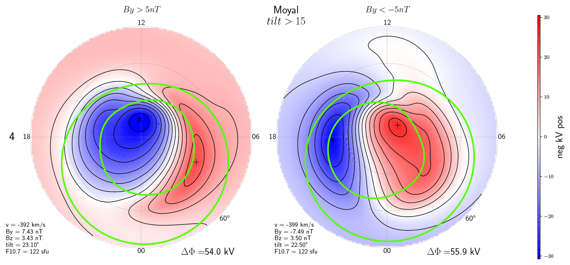
Figure 20 High-latitude convection cells with auroral boundaries (green lines). The left and right panels are for positive and negative IMF B_y, respectively, during local summer in the Northern Hemisphere. Auroral boundaries and solar wind conditions are those shown in Figs. 8 and 9 for the Moyal mean results for Dataset 4 (figure taken from Hessen, 2023).

Figure 21 Same as Fig. 20 but for local winter in the Northern Hemisphere. The boundaries are derived from the statistical mean. Auroral boundaries and solar wind conditions are those shown in Figs. 10 and 11 for the statistical mean results for Dataset 4 (figure taken from Hessen, 2023).

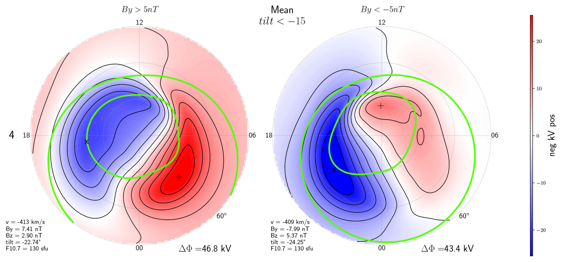
During local summer, the presence of IMF B_y causes one of the convection cells to become circular, while the other takes on a crescent shape. For positive IMF B_y, both the polar cap boundaries and the circular convection cell are displaced toward dawn; for negative IMF B_y, they are shifted toward dusk. In local summer, convection in the dawn-dusk direction primarily occurs within the polar cap boundaries, whereas in local winter, the convection inside the polar cap boundaries is oriented more directly anti-sunward.

Le et al. (2002) reported a single convection cell in the dayside polar cap, with clockwise flow driven by reconnection on open field lines primarily within the polar cap, while a second, nightside cell with counterclockwise flow circulates across the polar cap boundary. This is consistent with our results. The tilt-related convection differences also align with Pettigrew et al. (2010). During local winter, convection is predominantly across the polar cap from dayside to nightside, whereas during local summer, the cells are shifted more along the dawn–dusk direction, indicating enhanced circulation within the polar cap. They suggested that the seasonal differences may arise from a combination of altered reconnection topologies due to dipole tilt, such as lobe reconnection, and variations in ionospheric conductance driven by differing solar illumination. However, the formation of the lobe convection cell appears to be the most dominant effect.

In Reistad et al. (2021), similar convection patterns were found. During local winter, anti-sunward flow occurs inside the polar cap boundaries, while the return flow is mostly equatorward of those boundaries. In local summer, a larger portion of the return flow occurs within the polar cap boundaries. This is attributed to seasonal differences in lobe reconnection, because lobe reconnection imposes tension forces on the field lines, thereby producing seasonal asymmetries.

6 Conclusions

In this study we have investigated how strong IMF B_y in combination with the Earth's dipole tilt angle affect the location, intensity, and size of the auroral oval. Because of the different levels of solar illumination between seasons, we developed a separation method to better represent average auroral emissions under sunlit conditions.

We have shown that there is a substantial (∼500 km in the Northern Hemisphere and ∼430 km in the Southern Hemisphere) dawn-dusk shift in polar cap location associated with the sign of IMF B_y during local summer when comparing strong positive and strong negative IMF B_y. This shift in polar cap location is thought to be related to the seasonal change in lobe reconnection efficiency, as lobe reconnection with strong IMF B_y causes tension forces along the dawn/dusk meridian. We interpret the inferred changes in the poleward boundary of the auroral oval as the boundary between open and closed field lines being displaced due to this effect. This shift is not observed during local winter. To our knowledge, this seasonal dependence has not been reported previously, and is relevant for predictions of the auroral oval location.

We have also found that during local summer, positive IMF B_y leads to wider dusk oval compared to dawn in the Northern hemisphere. This is also true during local summer in the Southern Hemisphere but for opposite signs of IMF B_y. During local winter, the effect on the width is not seen in either Hemisphere. We suggest that this is related to the same mechanisms behind the dawn-dusk shift in the polar cap location, as they are present under the same conditions.

We have shown that in sunlit conditions the mean SSUSI EDR intensity is dominated by the dayglow residual and underestimate auroral intensities by 30 %–40 % (e.g., Fig. 19). Thus, we suggest that the separation method we have presented in Sect. 3.1 yields a better estimate of dayside auroral intensities during local summer, provided that one ensures the fits match the observed distributions.

The LBHS data from the EDR Aurora dataset have obvious challenges based on the functioning of the instrument and data processing, as can be seen in the extreme negative outliers and negatively biased dataset. This makes it difficult to use the distributions of auroral intensities to describe the underlying physical processes. However, this mainly applies to statistical estimates using these data and not for single events. Regarding the latter, there is in principle no limitation to the applicability of our method to individual events or images. The only requirement is that there be enough observations to form a statistically meaningful representation of the underlying intensity distribution.

As one of the shortcomings of our method is the assumption that the aurora follows the same distribution in the entire auroral oval, the separation method could be improved in the future by exploring if different PDFs could better explain the auroral distributions. As this study was limited to analyzing the Lyman-Birge-Hopfield short band in the SSUSI EDR Aurora data, future work could be determining if the method also work on the LBH-long band as well. Further investigation of the negative bias of the SSUSI dataset is also something that could improve the accuracy of our method.

To further examine if the lobe reconnection efficiency is the cause of the dawn-dusk shift in polar cap location, looking at periods with southward-directed IMF with significant IMF B_y could be useful. If a dawn-dusk shift in the polar cap is present under these conditions, it suggests that the lobe reconnection might not be the driving mechanism behind this effect, as lobe reconnection is not present when IMF B_z<0. MHD simulations could also be used to further validate or discard our findings.