A comparison of modeled daytime E regions from E-PROBED and PyIRI with ionosonde observations

While the F region is the primary focus of many ionospheric models because it contains the peak electron density, the E region is an important region for ionospheric conductivities and high-frequency radio propagation. This study analyzes modeled E regions from the newly developed PyIRI and E-PROBED models. A long-term comparison of E region predictions from E-PROBED and PyIRI with ionosonde observations is performed for three sites spanning low- (Fortaleza, Brazil), mid- (El Arenosillo, Spain), and high-latitudes (Gakona, Alaska). Modeled foE and hmE trends are compared against a combination of manually-scaled and automatically-scaled ionograms using ARTIST-5 for the period 2009–2024 for El Arenosillo and Gakona, and 2015–2024 for Fortaleza. Measured and modeled virtual heights are compared for a subset of the ionograms through the use of a numerical ray-tracer. Overall, the models showed reasonable agreement with the ionosonde observations, with solar cycle, seasonal, and diurnal trends well captured for foE. E-PROBED generally overestimates foE with Mean Absolute Relative Errors (MRAEs) peaking around 70 % at dusk, while PyIRI showed close agreement with ionosonde foE resulting in MRAE peaks around 10 %. The hmE predictions showed weaker agreement, with a 15-20 km overestimate from E-PROBED when compared against auto-scaled ionograms, and a constant hmE prediction of 110 km for all times from PyIRI. However, manually-scaled hmE estimates show close agreement with E-PROBED predictions, indicating that great care must be taken when using auto-scaled hmE. Modeled virtual heights derived from E-PROBED and PyIRI show reasonable agreement with ionosonde observations, providing confidence in altitude-integrated electron density profiles. A slight bias exists between the modeled and measured virtual heights, and the direction of the bias reverses for manual- versus auto-scaled ionograms, demonstrating that auto-scaled uncertainties are also present in the virtual height observations. Overall, these results indicate that E-PROBED and PyIRI provide reasonable E region estimates and may be used for practical applications that require modeled E region parameters.

1 Introduction

The E region of the ionosphere plays an important role in ionospheric conductivities (Rishbeth and Garriott, 1969; Kelley, 2009) that impact ground-based magnetometer observations (Brekke et al., 1974; Yamazaki and Maute, 2017), atmospheric energy input and balance (Roble et al., 1987), and High Frequency (HF) radio propagation (Fabrizio, 2013). Therefore, a proper understanding of global E region morphology can provide insight into both scientific and practical applications, especially through the use and development of E region models.

Critical frequencies of the E region (foE; or corresponding peak electron density NmE) have been studied for many years, revealing a relationship with the solar zenith angle (Muggleton, 1972), season (Kouris and Muggleton, 1973b), sunspot number (Muggleton, 1971b), and Sun-Earth distance (Muggleton, 1971a). Global collections of ionosondes have provided insight into foE variation over time, such that empirical relationships could be developed (e.g., Kouris and Muggleton, 1973a; Kouris, 1998). Similarly, rocket and incoherent scatter radar data have been used to calculate empirical NmE trends (Chasovitin et al., 1985). As the E region is photochemistry dominated and driven primarily by extreme ultraviolet (EUV) flux with wavelengths below 150 Å (Schunk and Nagy, 2009), chemistry models have been created (Titheridge, 1996, 1997), providing insight into difficult-to-measure densities (such as [NO]) and reaction rates and coefficients.

Models of the peak electron density altitude of the E region, hmE, have also been developed (Ivanov-Kholodny et al., 1998; Titheridge, 2000). These studies have shown that hmE remains nearly constant around local noon at lower altitudes, with increases in altitude near sunrise and sunset. The general behavior of hmE can be captured by Chapman theory (Chapman, 1931), providing a linear relationship with the natural log of the secant of the solar zenith angle. Titheridge (2000) derived a modified Chapman theory dependence for hmE taking into account season, latitude, solar flux, solar zenith angle and local time, resulting in hmE values between 105 and 120 km that agree well with ionosonde observations from Auckland, New Zealand.

A Chapman-layer E region can be approximated as a quasi-parabola (Bradley and Dudeney, 1973), requiring a peak altitude, peak density, and half-thickness (scale height) to describe the bottomside shape. These parameters can be calculated using virtual height measurements from ionosondes (Reinisch and Xueqin, 1983; Titheridge, 1985a), making ionosondes a powerful tool for extracting E region electron density profiles (EDPs). For this reason, long-term ionosonde observations have been used as the backbone of global bottomside E region models such as the empirical International Reference Ionosphere (IRI; Bilitza, 1990, 1998. While Incoherent Scatter Radar (ISR) observations contribute to IRI's estimates for the E-F valley, foE and hmE are mainly driven by ionosonde observations (Bilitza et al., 2022). Recently, the core framework of IRI has been implemented in Python instead of the historical Fortran approach in the new PyIRI (Forsythe et al., 2024), allowing for more rapid execution of global ionospheric profiles. Similar to the core of the IRI model, PyIRI uses the global Consultative Committee on International Radio (CCIR) and the International Union of Radio Science (URSI) coefficients for foF2 and the HF propagation parameter M(3000)F2 (Maximum Usable Frequency for a distance of 3000 km normalized to foF2) that can be used to calculate hmF2 (Bilitza and Eyfrig, 1979). PyIRI currently implements the standard options from IRI while also using certain features of NeQuick (Nava et al., 2008) for the top-side and E region such that the overall model is a combination of IRI and NeQuick. This results in nearly identical results between PyIRI and IRI-2020 for certain parameters such as hmF2, while producing different EDP shapes due to the NeQuick features and differences in EDP construction (Forsythe et al., 2024). Although the focus of the present study is on the E region, IRI provides an empirical estimate of the entire ionosphere (all ionospheric altitudes), resulting a quick and easy-to-run model widely used by the ionospheric community.

With recent improvements in Global Navigation Satellite System (GNSS) Radio Occultation (RO) techniques for extracting D and E region electron densities (Wu, 2018), global E region observations are now available in regions that were previously unobtainable by ionosondes or ISR (Wu et al., 2022, 2023). GNSS-RO provides horizontally integrated observations of the ionosphere and atmosphere, using signals of opportunity from GNSS and a Low Earth Orbit (LEO) satellite to receive the signals (Schreiner et al., 1999b), resulting in a large and globally distributed observational dataset for the ionosphere (e.g., CDAAC, 2025). These global GNSS-RO observations have been used to develop a modern E region model, E region Prompt Radio Occultation Based Electron Density (E-PROBED; Salinas et al., 2024). The model was developed using Constellation Observing System for Meteorology, Ionosphere, and Climate (COSMIC-1) observations of the E region from 2007–2016 and is driven by Solar Zenith Angle (SZA), season, and F10.7 with an additional non-SZA component that is a function of latitude, local time, season, and F10.7 (Salinas et al., 2024). Time series of NmE, hmE, and scale-height for each latitude-local time bin were fit to Fourier coefficients up to the 10th harmonic, providing a lookup table for each bin that is called within E-PROBED. GNSS-RO derived EDPs used to drive E-PROBED were estimated using a bottom-up approach that limits F region contributions through a weighting function with minimal contributions from higher altitudes, unlike the standard Abel transform typically used for RO inversion (Wu, 2018; Wu et al., 2022). Ultimately, this global GNSS-RO dataset provides a novel method for estimating bottomside EDPs, with E-PROBED encompassing the observations into an empirical model that can predict global E region EDPs for altitudes between 90–120 km.

While the truly global spread of GNSS-RO observations provides great promise for remote sensing of the upper atmosphere, the integrated nature of the measurements (Hajj and Romans, 1998; Schreiner et al., 1999a) motivates the need for additional comparison against more direct observations such as those implemented by ionosondes. The same argument holds for models derived from GNSS-RO (E-PROBED) versus ionosonde (PyIRI) observations of the E region. A recent study by Shaver et al. (2023) has provided a framework for this comparison between EDPs derived from GNSS-RO, ionosondes, and models. In the present study, we implement many of the same approaches to compare modeled E regions from E-PROBED and PyIRI to ionosonde observations used as the “ground-truth” validating dataset. This effort aims to provide insight into model performance as well as the solar cycle, seasonal, and diurnal morphology of the E region for several ionosonde sites spanning low-, mid-, and high-latitudes.

2 Materials and methods

Three Digisonde sites were selected as the basis for this comparison: Fortaleza, Brazil (URSI code FZA0M, 3.9° S, 321.6° E, −21.5° inclination), El Arenosillo, Spain (EA036, 37.1° N, 353.3° E, 50.6° inclination), and Gakona, USA (GA762, 62.4° N, 215.0° E, 75.5° inclination). These three sites span low-, mid-, and high-latitudes, providing a comparison over a variety of ionospheric conditions. Ionosonde virtual height observations, foE, and hmE estimates were obtained from the Digital Ionogram Database (DIDBASE, 2025). Virtual heights were obtained using SAOExplorer version 3.6.1 (SAO-X, 2025) while the foE and hmE estimates were downloaded directly from DIDBASE. The virtual height observations have a frequency resolution of approximately 25 kHz and Digisondes use a standard temporal resolution of one ionogram every 15 min. However, the temporal resolution can be variable, sometimes increasing up to 5 min per ionogram. In addition, there are several periods with outages at each site, which can last anywhere from days to years. It should also be noted that the minimum foE observations from ionosondes are constrained by the minimum transmit frequency and sensitivity, such that nighttime foE values below ∼1.5 MHz are generally not measured by ionosondes. Therefore, the comparison performed here does not include nighttime observations or model estimates.

To provide a long-term comparison, automatically-scaled ionograms using the Automatic Real-Time Ionogram Scaler with True Height calculation version 5 (ARTIST-5; Galkin and Reinisch, 2008) were used for foE and hmE estimates. The start dates for implementing ARTIST-5 vary from site to site, with El Arenosillo implementing in December 2008, Fortaleza in November 2014, and Gakona in May 2007. From this, the foE and hmE comparison for each site begins on the date of ARTIST-5 implementation and continues through 2024. Within each of these periods, a collection of manually-scaled ionograms are also available, with the largest density for EA036 in 2009.

Although auto-scaled ARTIST-5 ionograms are known to differ from manually-scaled profiles (e.g., Stankov et al., 2023), the use of auto-scaled ionograms allows for a prolonged comparison period to analyze long-term trends. In an attempt to remove poor quality ionograms from the comparison, ARTIST confidence scores were required to be above 90 %. While it is not entirely clear how these confidence scores map to an uncertainty in electron density as a function of altitude, the 90 % confidence threshold requires a series of quality control criteria to be satisfied such that noisy or problematic ionograms are removed (Galkin et al., 2013; Themens et al., 2022). Furthermore, we implemented additional criteria to be satisfied as an expanded quality control procedure: the foE was required to be above the minimum transmitted frequency, fmin, profiles with sporadic-E (foEs) observations were removed, hmE values were required to be above 90 km, and hmE estimates of exactly 110 km were removed. The removal of 110 km hmE values was implemented because of a large number of ionograms that defaulted to this altitude, likely following climatological estimates and not derived entirely from the observations. This 110 km hmE altitude will be discussed in more detail in Sects. 3 and 4.

Geomagnetically quiet conditions were also enforced for the comparison by constraining Kp ≤3, with Kp values obtained from NASA's OMNIWeb (Papitashvili and King, 2020). This ensures that differences in E region observations and model predictions are not reliant on the model's ability to predict variations caused by geomagnetic activity. Both E-PROBED and PyIRI were run for each ionogram time satisfying the criteria outlined above. In total, this results in 19 727 foE and hmE observations for EA036 (including 896 manually-scaled ionograms), 54 036 for FZA0M, and 3837 for GA762.

For the models, E-PROBED version 1.0 (Salinas, 2024) was used to estimate E region EDPs using longitude, latitude, altitude range (90–130 km with 0.25 km resolution), date, and time of day as input. The foE and hmE estimates were calculated from the EDPs using Scipy's find_peaks function (Virtanen et al., 2020), that performed well on the smooth E-PROBED profiles with a single E region peak. PyIRI profiles were calculated using version 0.0.2 (Forsythe and Burrell, 2023) with an altitude range of 90–130 km and a resolution of 0.25 km. The PyIRI inputs are longitude, latitude, date, time of day, F10.7, altitude range, and an option for NmF2 calculations, ccir_or_ursi, which was set to use the CCIR coefficients. The foE and hmE values were output directly from PyIRI.

Although foE can be observed directly from virtual height observations as an E region cusp (assuming foE is outside of a restricted transmission band), hmE estimates are calculated through a quasi-parabolic fit to the virtual height data (e.g., Titheridge, 1985b; Reinisch and Xueqin, 1983), which results in additional uncertainty for the hmE estimates. To account for this additional uncertainty in the altitude estimates, a comparison to directly measured ionogram virtual heights is performed on a subset of the data. Virtual height observations contain information on the shape and magnitude of EDPs through the group index of refraction (Budden, 1966), which provides a more direct comparison against ionosonde observations than comparing against inverted EDPs that require a series of assumptions on the profile shape, etc. (Shaver et al., 2023). The E-PROBED and PyIRI EDPs were converted to virtual heights through the use of a High Frequency (HF) ray tracer. Specifically, the EPDs were input into Another Ionospheric Ray Tracer (AIRTracer; a model developed by Eugene V. Dao at the Air Force Research Laboratory) to calculate virtual heights for ordinary-mode rays. AIRTracer uses the Jones-Stephenson (Jones and Stephenson, 1975) formulation with the Booker quartic and no collisions, and has been rewritten in the Julia Programming Language to decrease computation time. For each subset of ionograms used for the virtual height comparison, a group path is calculated for each transmit frequency of the ionogram virtual height data (roughly 25 kHz resolution) using the E-PROBED and PyIRI EDPs. The virtual height is then taken as half of the group path. Due to the additional processing time required to calculate the virtual heights of E-PROBED and PyIRI, the observation subset was limited to January-March 2009 for EA036 (total of 618 profiles), August 2019 for FZA0M (711 profiles), and May 2008 to January 2009 for Gakona (515 profiles). These periods were selected when the data density was large for the site of interest, and the period selected for EA036 includes the manually-scaled ionograms. A total of at least 500 profiles was desired for each site, which resulted in variable time spans due to differences in ionogram cadence and quality (i.e., lack of ionospheric disturbances, etc.).

3 Results

The comparison results are separated by the ionosonde site, and the combined trends will be discussed in Sect. 4. For each site, the trends are analyzed by year (solar cycle), day of year (seasonal), and solar local time (diurnal), with seasonal and diurnal results displayed in Appendix A. Then, the modeled virtual heights predicted by E-PROBED and PyIRI are compared with ionosonde observations for a subset of the ionograms.

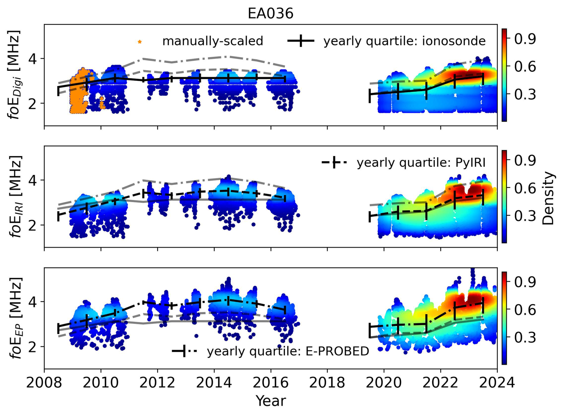
Figure 1 Yearly foE estimates for El Arenosillo using ionograms (top), PyIRI (middle), and E-PROBED (bottom). The manually-scaled ionograms are marked with orange stars, and the color represents the normalized data density. Black trend lines intersect the yearly medians, with quartiles (25 % and 75 %) shown as error bars. For comparison, semi-transparent lines show the median trends for the other two datasets.

3.1 El Arenosillo, Spain

The yearly foE estimates for El Arenosillo, Spain (EA036) are shown in Fig. 1, spanning from December 2008 to 2024. Manually-scaled ionograms are marked by orange stars to distinguish from the auto-scaled ionograms, with the majority of manually-scaled ionograms taking place in 2009. For foE, the manually-scaled trends match the auto-scaled trends due to the E region cusp in ionograms, which provide a direct feature to estimate foE (e.g. Fig. 1.3 of Piggott and Rawer, 1961).

Yearly quartiles are calculated for each dataset to show long-term trends. In Fig. 1, the black trend lines intersect the yearly medians, and the 25 % and 75 % quartiles are shown as error bars for each year. The ionosonde observations show a slight increase during Solar Cycle 24 with median foE values of 3.1 MHz for 2014 and a range of 1.7–3.4 MHz. As mentioned previously, nighttime foE observations fall below the minimum frequency measured by ionosondes, fmin, such that the minimum foE observations do not include nighttime values. The median decreased to 2.5 MHz during solar minimum near 2020 with a sharp increase to 3.2 MHz in 2023 along with an extended range of 1.6–4.0 MHz. Seasonal trends are clearly visible with peaks in the local (boreal) summer, with an interesting double peak surrounding the summer of 2023 (upper right of Fig. 1). A more in-depth discussion of seasonal and diurnal trends is provided in Appendix A.

E-PROBED and PyIRI show a more pronounced solar cycle trend around solar maximum in 2014. The median foE in 2014 for PyIRI is 3.5 MHz with a range of 1.8–4.2 MHz. Similarly, E-PROBED predicted a median foE of 4.1 MHz with a range of 2.3–5.0 MHz around 2014. A sharp increase in foE values is observed from 2020 to 2023 for both PyIRI and E-PROBED, which is consistent with the ionosonde trend. In general, $\mathit{fo}{\mathrm{E}}_{\mathrm{EP}}>\mathit{fo}{\mathrm{E}}_{\mathrm{IRI}}>\mathit{fo}{\mathrm{E}}_{\mathrm{Digi}}$, with a larger difference between E-PROBED and ionosondes during Solar Cycle 24 compared to Solar Cycle 25. Both PyIRI and E-PROBED predict multiple spikes in 2023, likely driven by the wide variations in F10.7 ranging from 115–335 sfu during the year. The large foE spike near 5 MHz for E-PROBED in early 2023 corresponds to the observed 335 sfu spike in F10.7. PyIRI's foE calculation goes as F10.7${}^{\mathrm{1}/\mathrm{4}}$ (Eq. 15 of Forsythe et al., 2024), which helps to reduce the impact of this F10.7 spike, better matching the observed ionosonde trends.

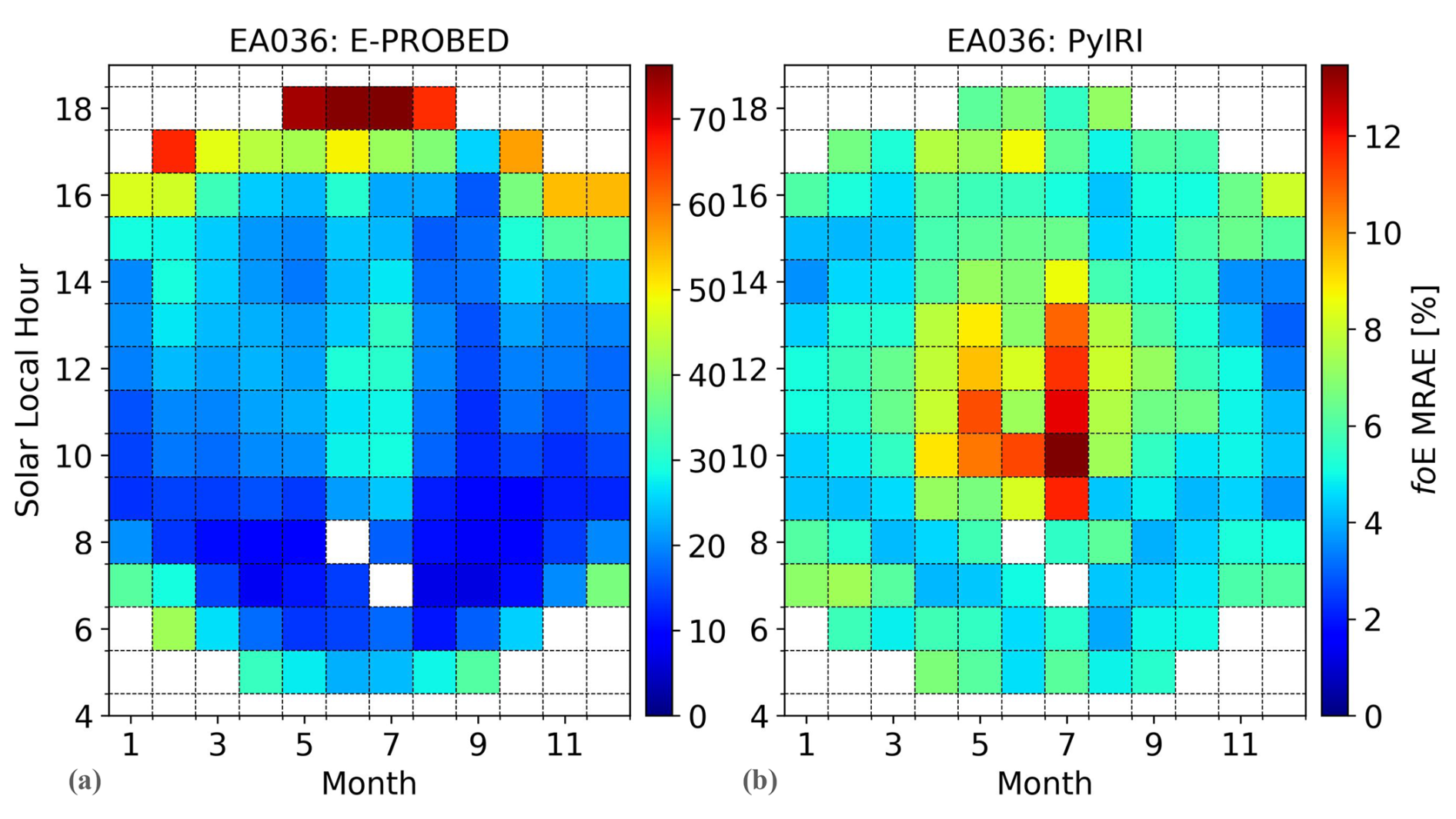
Figure 2 Mean Relative Absolute Error (MRAE) for foE predictions by (a) E-PROBED and (b) PyIRI at El Arenosillo. Peak MRAE of 76 % is observed near dusk during local summer for E-PROBED while PyIRI MRAE peaks at 13 % near noon during summer. Note the change in scale between the two subfigures.

Mean Relative Absolute Error (MRAE) calculations were performed for foE following $\mathrm{MRAE}=|\mathit{fo}{\mathrm{E}}_{\mathrm{model}}-\mathit{fo}{\mathrm{E}}_{\mathrm{obs}}|/\mathit{fo}{\mathrm{E}}_{\mathrm{obs}}$. Due to the wide range of errors between models over time and the fact that both models tend to overestimate foE, the absolute error was computed instead of the signed error so that log (MRAE) could be displayed for comparison. The MRAE was averaged for each month and solar local hour bin, with at least 10 points required for the bin to display a result. As shown in Fig. 2, E-PROBED has the largest relative errors near dusk during local summer, with a peak MRAE of 76 %. Dawn and summertime noon also have larger errors for E-PROBED, and the mean MRAE over all times is 24 % due to the overestimated foE magnitudes shown in Fig. 1. The MRAE for PyIRI are very low in comparison, with peak MRAE of 13 % during summertime noon and a time-averaged MRAE of only 6 %.

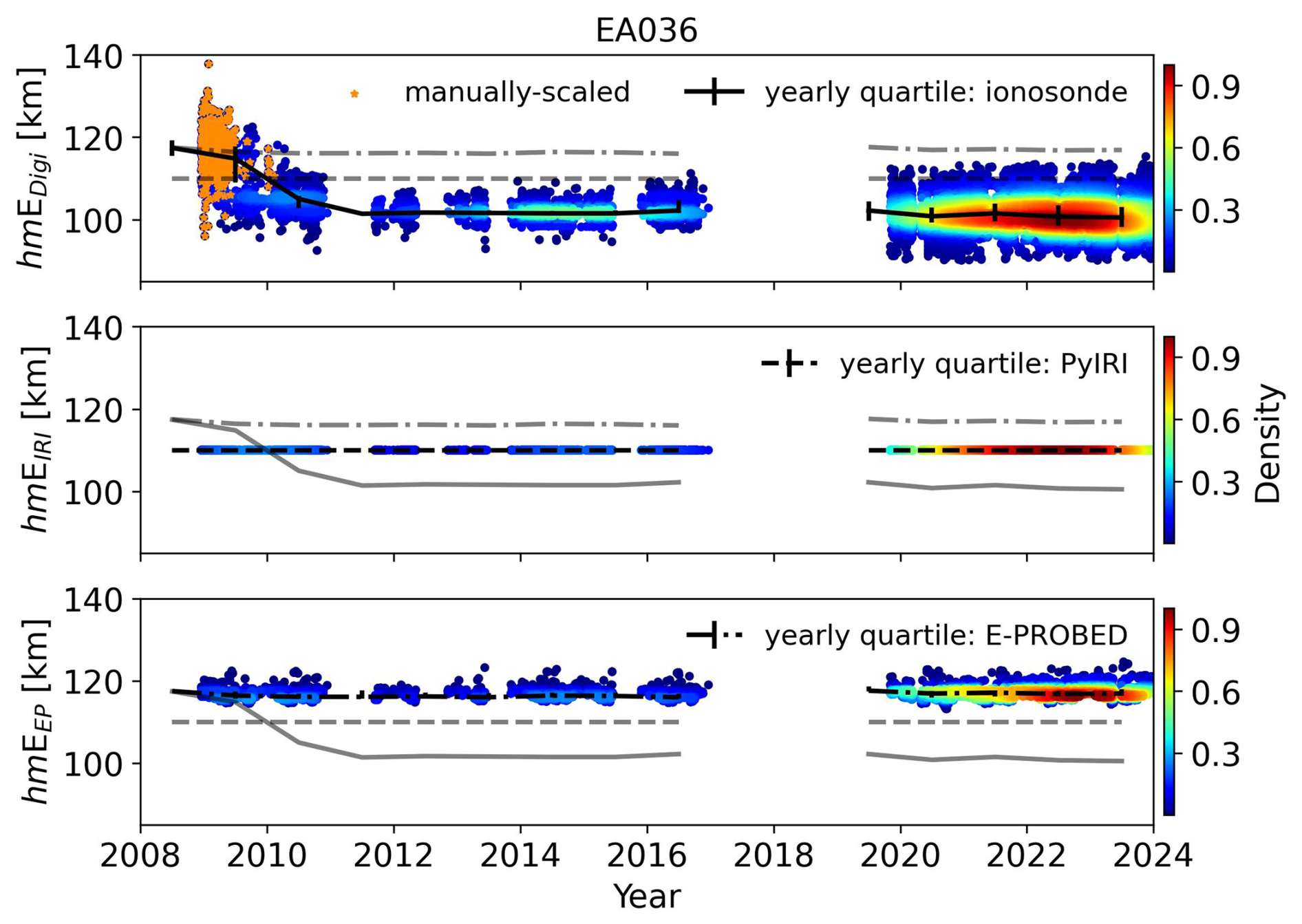
Figure 3 Yearly hmE estimates for El Arenosillo using ionograms (top), PyIRI (middle), and E-PROBED (bottom). Black trend lines intersect the yearly medians, with quartiles (25 % and 75 %) shown as error bars. For comparison, semi-transparent lines show the median trends for the other two datasets.

While foE can be estimated directly from E region cusps in ionograms, hmE requires a best-fit to the entirety of the E region observations. This difference will be explored in more detail in Sect. 4, but it is important to point out that the relative uncertainty in hmE estimates from ionosondes is generally greater than the foE uncertainties due to the assumption of a parabolic bottomside E region profile for a Chapman layer and the best-fit procedure required to extract the peak frequency, height, and layer thickness (Reinisch and Xueqin, 1983; Titheridge, 1985a). From this, while the manually-scaled foE estimates were consistent with the auto-scaled estimates, the manually-scaled hmE estimates show significant differences with the auto-scaled values. This difference is readily observed in the yearly hmE trends shown in Fig. 3. In 2009, the observations with a large collection of manually-scaled ionograms show median hmE values near 115 km, with a significant drop to values near 100 km for the remainder of the comparison period for the auto-scaled ionograms. Manually-scaled ionogram hmE values range from 95–135 km, while the auto-scaled ionograms range from 90–115 during Solar Cycle 25. As manually-scaled ionograms are deemed more trustworthy than auto-scaled ionograms, long-term hmE trends after 2009 must be viewed with caution. Ideally, a long-term collection of manually-scaled ionograms spanning several years should be used for a future comparison to remove the uncertainties inherent with auto-scaling, but here we rely on the available Digisonde dataset with a limited collection of manually-scaled ionograms while pointing out that the displayed hmE trends appear to be more susceptible to errors than foE trends.

The solar cycle variation is less pronounced for hmE, but seasonal trends show peaks in the local (boreal) winter that match the expected reciprocal relationship expected between foE and hmE for a Chapman layer (Chapman, 1931). E-PROBED hmE predictions also show a less pronounced solar cycle variation compared to foE. The median hmE predictions from E-PROBED are consistently around 115 km, which agrees with the manually-scaled ionograms. E-PROBED shows less variation, however, with most predictions between 115–120 km.

PyIRI predicts a constant value of 110 km for all conditions and times in this comparison. For this reason, the PyIRI hmE are not displayed in the remaining figures. However, it should be noted that the large number of ionograms removed during quality control with hmE =110 km follows from the starting point of 110 km for hmE, as suggested by the Committee Consultative for Ionospheric Radiowave Propagation (CCIR) during ionogram inversion with ARTIST (Bradley and Dudeney, 1973; Reinisch et al., 1988). Given the large difference between manually-scaled and auto-scaled ionogram hmE estimates along with the constant PyIRI hmE value, the remaining hmE figures for all sites are reserved for Appendix A.

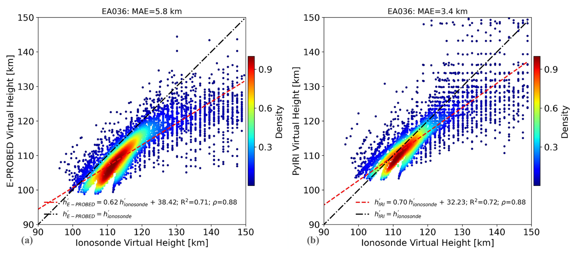
Figure 4 Modeled virtual heights from (a) E-PROBED and (b) PyIRI compared against ionosonde observations for El Arenosillo. Observations from 618 (528 manually-scaled) ionograms are displayed spanning January–March 2009.

While foE and hmE are helpful parameters to characterize the peak of the E region, they do not inherently contain information on the shape of the E region profile. However, virtual height observations provide a method for model comparison that depends on both profile shapes and magnitudes. Since the ionosonde virtual heights are direct observations, this removes the uncertainties created during the ionogram inversion process to provide a more direct comparison with measurements. Virtual heights for an individual layer (e.g., E layer) are expected to monotonically increase, but the rate of increase depends on the spatially integrated group index of refraction, which is a function of the electron density over altitude (Budden, 1966). From this dependence, differences in electron density magnitudes, altitudes, and shapes will result in virtual height differences such that calculated virtual heights can be used as a validating metric for modeled EDPs that is free from uncertainties incurred by profile shape assumptions used during ionogram inversion (Shaver et al., 2023).

The virtual heights derived from E-PROBED and PyIRI over EA036 are shown in Fig. 4 compared to ionosonde observations. The period of January–March 2009 was selected for comparison because it contained a large density of manually-scaled ionograms (528 of the 618 total). Each point in the figure corresponds to the virtual height measured by the ionosonde and the modeled virtual height using the transmitted ionosonde frequency for all frequencies below foE in each individual ionogram. With the roughly 25 kHz transmit frequency resolution, this corresponds to nearly 8000 datapoints for comparison.

Both PyIRI and E-PROBED match the ionosonde observations fairly well, with R² values of 0.7 and a Spearman's rank correlation coefficient, ρ, of 0.9 for both. The overall agreement is better for PyIRI with a Mean Absolute Error (MAE) of 3 km and a linear fit slope of 0.7 while E-PROBED produces an MAE of 6 km and a slope of 0.6. Both models show a slight underestimation for the majority of predictions, and the reduced linear fit slope for E-PROBED is due to a collection of underestimated virtual heights for ionosonde virtual heights above 130 km. This underestimation stems from the slight overestimation of foE values, which pushes the modeled foE cusps to frequencies higher than those observed in the ionosondes. The larger virtual heights correspond to frequencies approaching the E region cusp, such that variations in foE can map to relatively large errors in virtual heights.

Interestingly, the virtual height predictions from PyIRI align very well with the observations, likely due to the close agreement in foE even though a constant hmE value of 110 km is estimated for every profile. As virtual heights are dependent on the integral of the altitude (z) gradient with respect to the plasma frequency (f_p), $\mathrm{d}z/\mathrm{d}{f}_{\mathrm{p}}$, the shape of the profiles plays an important role (Budden, 1966). From this, an underestimation bias in hmE by PyIRI (see manually-scaled ionogram data in Fig. 3) can be compensated for with elevated $\mathrm{d}z/\mathrm{d}{f}_{\mathrm{p}}$ for a given transmit frequency to produce similar virtual heights. This $\mathrm{d}z/\mathrm{d}{f}_{\mathrm{p}}$ is a function of foE and layer semi-thickness, which are, in fact, adjusted during ionogram inversion to match observed virtual heights (Reinisch et al., 1988).

3.2 Fortaleza, Brazil

To avoid duplicated discussion, we focus on comparing and contrasting trends with EA036 instead of focusing on specific values in the discussion below. The yearly foE trends for FZA0M follow the same trends as observed over EA036 with a clear solar cycle variation showing elevated foE values during solar maximum (Fig. 5). E-PROBED foE estimates are greater than PyIRI and ionosonde values, while the latter two are nearly equal on average. A spike is observed in September 2017 for both E-PROBED and PyIRI when F10.7 increased to 185 sfu. However, this foE spike is not observed in the ionograms. It must be noted that this equatorial region is prone to E region ionospheric irregularities from equatorial electrojet instabilities (Arras et al., 2022) and particle precipitation allowed by the South Atlantic Anomaly (Moro et al., 2022), which can cause additional uncertainties in ionogram auto-scaling.

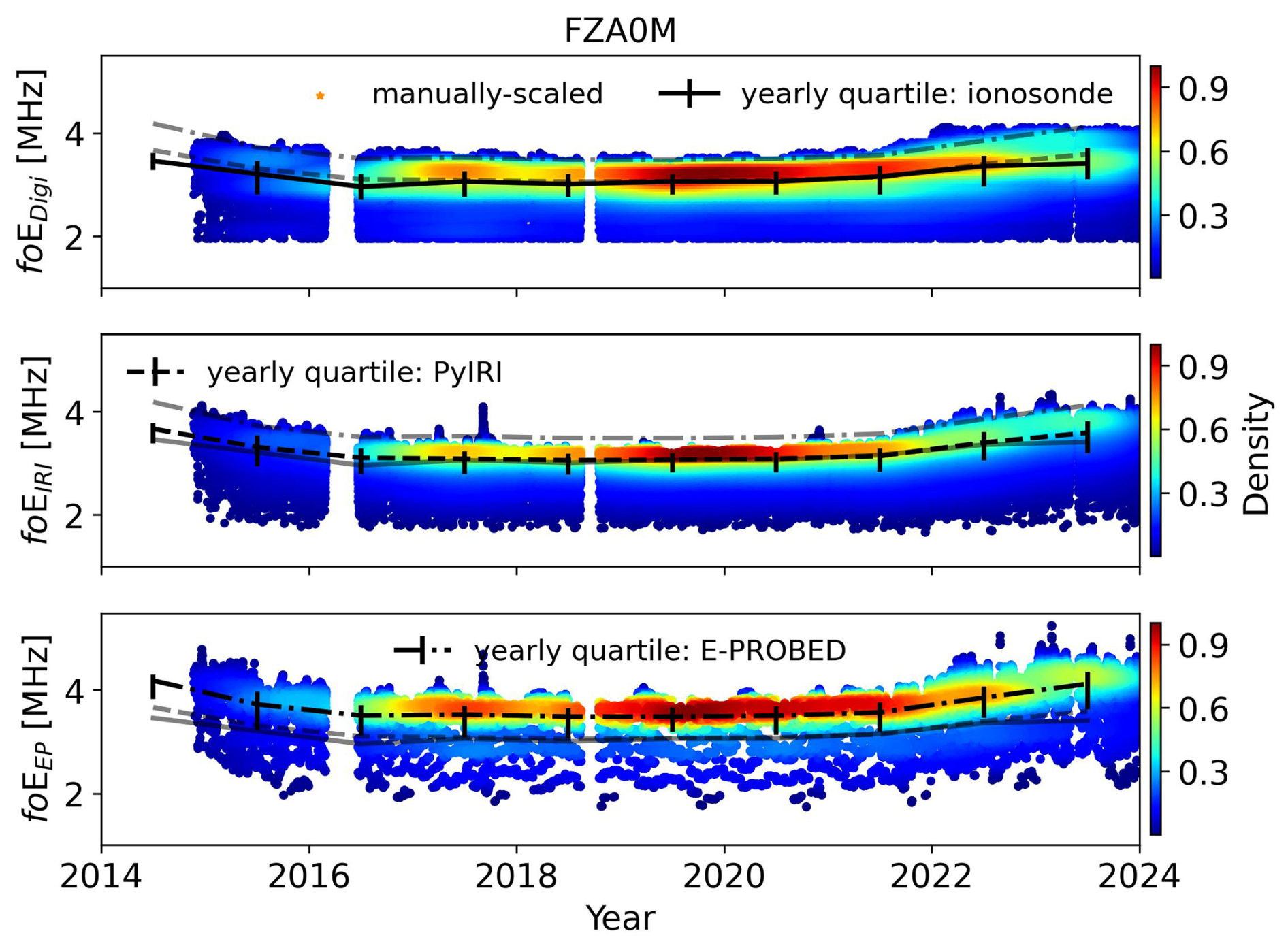
Figure 5 Yearly foE estimates for Fortaleza using ionograms (top), PyIRI (middle), and E-PROBED (bottom). Black trend lines intersect the yearly medians, with quartiles (25 % and 75 %) shown as error bars. For comparison, semi-transparent lines show the median trends for the other two datasets.

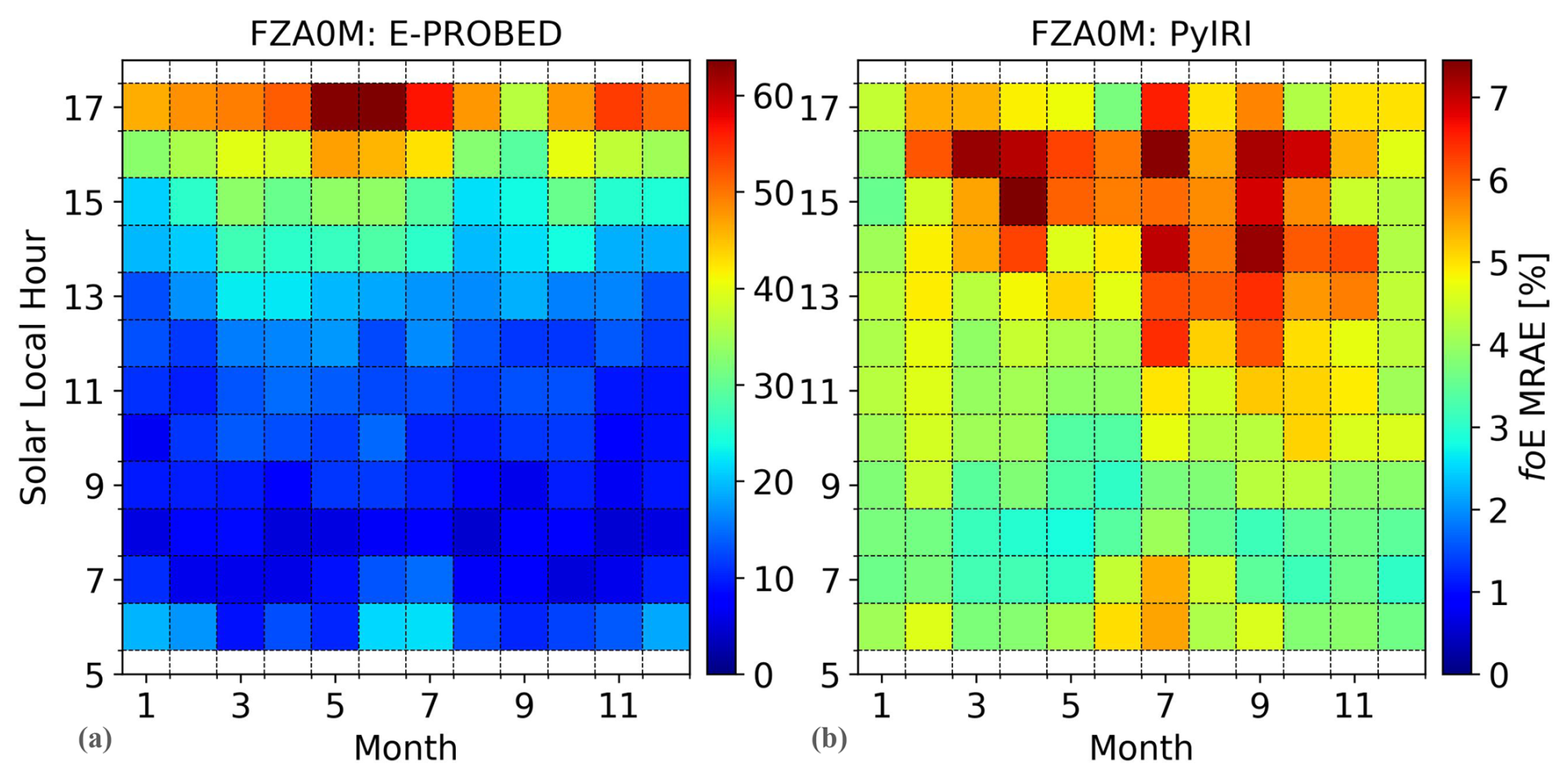
Figure 6 Mean Relative Absolute Error (MRAE) for foE predictions by (a) E-PROBED and (b) PyIRI at Fortaleza. Peak MRAE of 64 % is observed near dusk for E-PROBED while PyIRI MRAE peaks at 7 % in the afternoon. Note the change in scale between the two subfigures.

MRAE calculations for modeled foE are shown in Fig. 6. Similar to EA036, E-PROBED shows larger relative errors with a peak MRAE of 64 % at dusk and a time-averaged MRAE of 19 %. The PyIRI errors are much lower, peaking at 7 % during the afternoon with a time-averaged MRAE of 5 %. Seasonal MRAE variations are less pronounced, as expected for this equatorial site.

Due to ambiguities between manually-scaled and auto-scaled hmE, the yearly hmE trends are reserved for Appendix A. For the virtual height comparison, a total of 711 ionograms from August 2019 were used as the ground-truth (Fig. 7). While the mid-latitude EA036 site showed relatively strong agreement between the modeled and measured virtual heights for both E-PROBED and PyIRI (Fig. 4), the equatorial FZA0M virtual height agreement is weaker. A linear fit of the E-PROBED virtual heights produces a slope of approximately 0.5 with an R² of 0.6, a Spearman's rank correlation coefficient of 0.8, and an MAE of 5 km. PyIRI produces similar R² and Spearman's rank correlation coefficient values, but with an MAE of 7 km and a linear fit slope of 0.6.

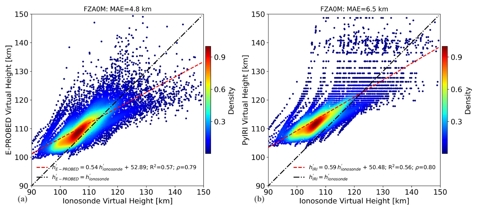
Figure 7 Modeled virtual heights from (a) E-PROBED and (b) PyIRI compared against ionosonde observations for Fortaleza. Observations from 711 ionograms are displayed spanning August 2019.

Both E-PROBED and PyIRI show a positive virtual height bias, unlike the negative bias produced for EA036. This change is related to the difference in manually-scaled vs. auto-scaled ionogram hmE estimates, where the manually-scaled hmE for EA036 are ∼15 km above the corresponding auto-scaled estimates. This reduction in ionosonde hmE corresponds to reduced virtual heights, thereby creating a positive bias in the modeled virtual heights for FZA0M.

3.3 Gakona, United States

Similar to the previous subsection, here we focus on general trends and differences between GA762 results and the results of EA036 and FZA0M. As observed in Fig. A8, the foE estimates for both PyIRI and E-PROBED show solar cycle trends similar to those of the ionosonde observations. However, from 2022–2024, E-PROBED predicts a steady increase in foE while the ionosonde and PyIRI trends remain flat over time. As for the previous sites, E-PROBED slightly overpredicts foE while PyIRI is nearly equal (with a very slight positive bias). It should be noted that the dynamic ionization contribution from precipitating electrons (Solomon, 1993) is difficult to capture in climatological models (Themens and Jayachandran, 2016), such that periods with elevated electron flux may reduce the gap between model overpredictions and ionosonde foE observations.

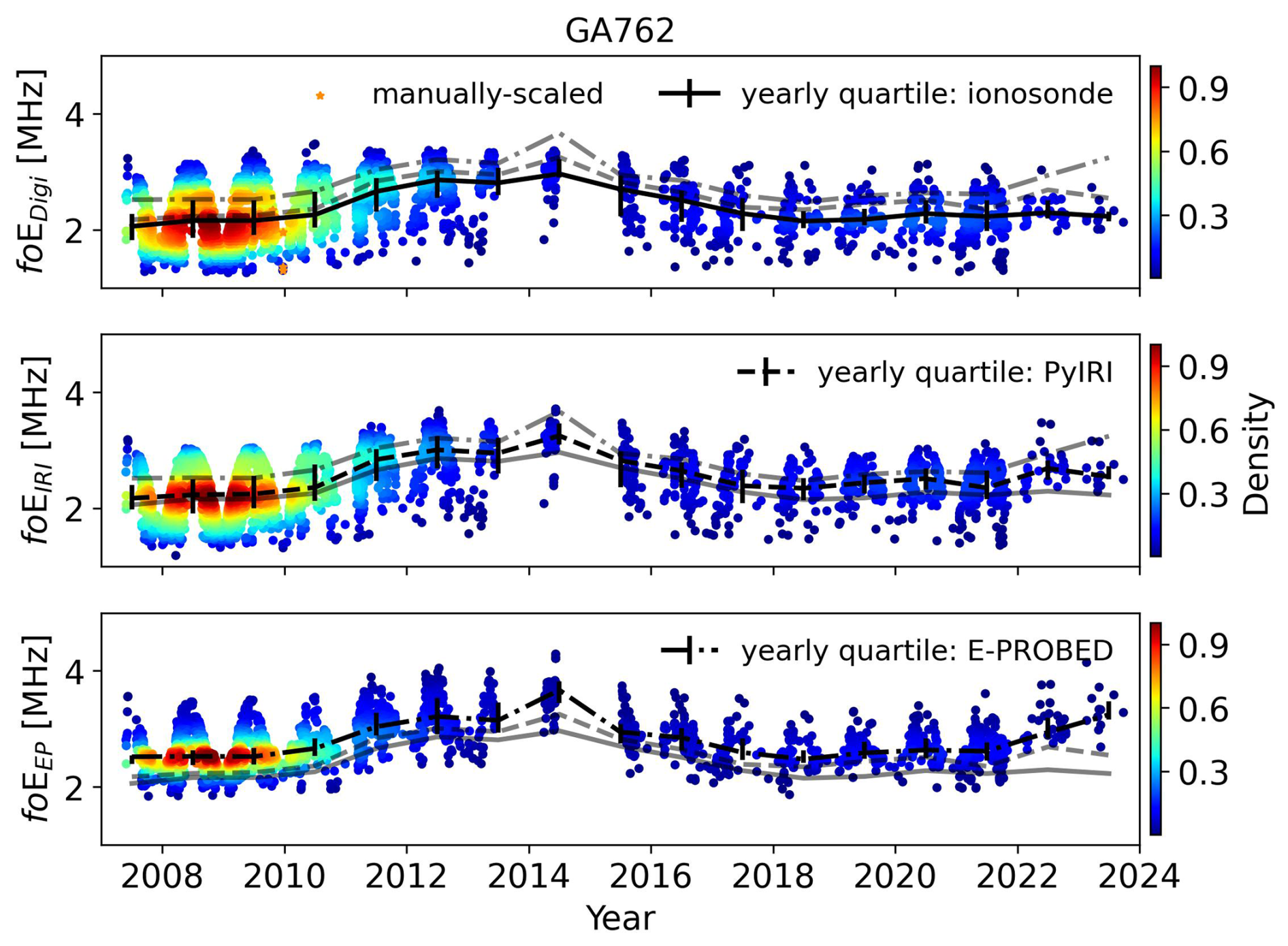
Figure 8 Yearly foE estimates for Gakona using ionograms (top), PyIRI (middle), and E-PROBED (bottom). Black trend lines intersect the yearly medians, with quartiles (25 % and 75 %) shown as error bars. For comparison, semi-transparent lines show the median trends for the other two datasets.

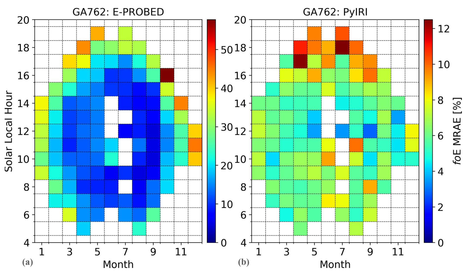
Figure 9 Mean Relative Absolute Error (MRAE) for foE predictions by (a) E-PROBED and (b) PyIRI at Gakona. Peak MRAE of 58 % is observed near dusk during autumn for E-PROBED while PyIRI MRAE peaks at 12 % near dusk in the summer. Note the change in scale between the two subfigures.

MRAE for the foE predictions are shown in Fig. 9. For Gakona, E-PROBED shows the largest MRAE of 58 % near autumnal dusk while also showing large errors near dusk throughout the year. PyIRI produces peak MRAE of 12 % near summertime dusk, with a low time-averaged MRAE of 7 % compared to 19 % for E-PROBED.

Modeled virtual heights for GA762 show a slightly larger slope of 0.6 for the E-PROBED predictions compared to 0.5 for PyIRI (Fig. 10). However, the E-PROBED predictions also show more variance with lower R² and ρ, mostly caused by the spread in the predictions and measurements for larger virtual heights above 130 km. This wider variance maps to a slightly larger MAE of 7 km for E-PROBED compared to the 6 km for PyIRI.

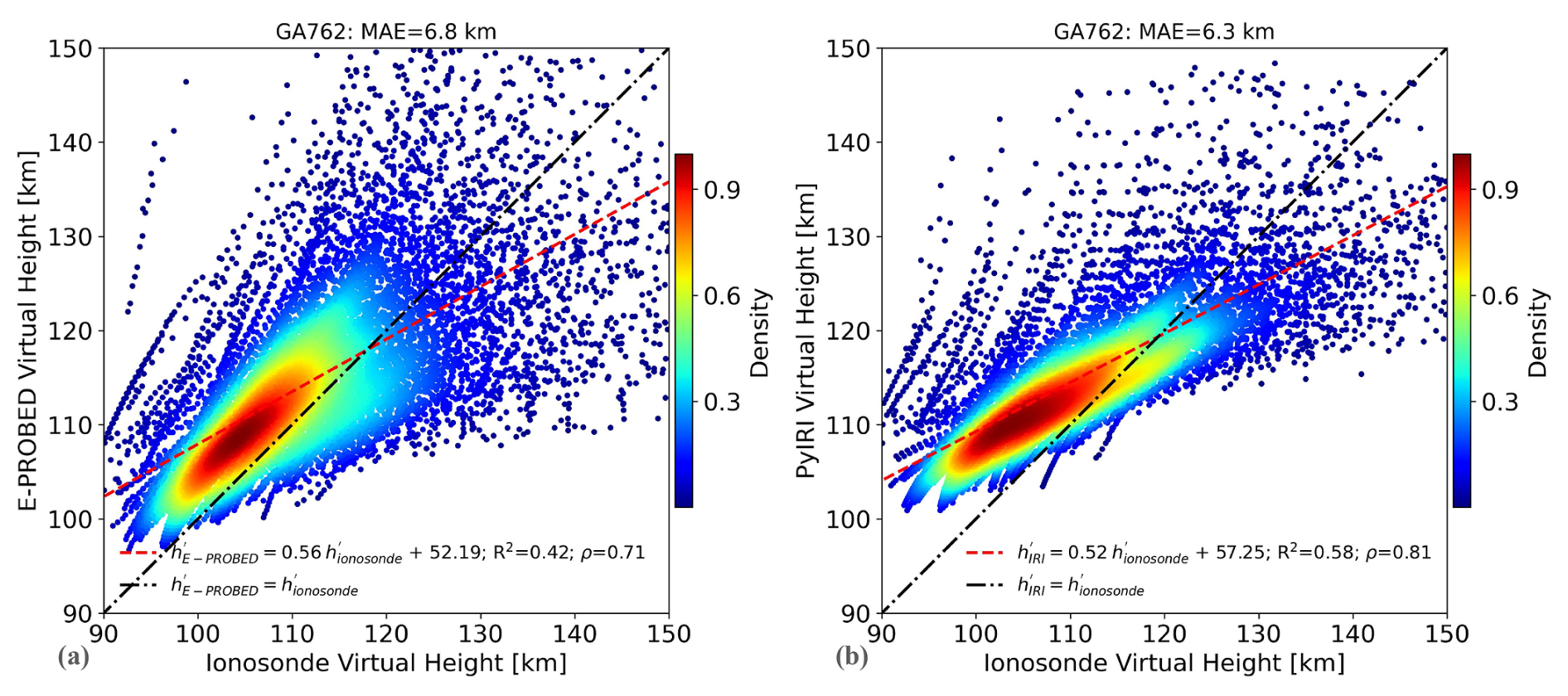
Figure 10 Modeled virtual heights from (a) E-PROBED and (b) PyIRI compared against ionosonde observations for Gakona. Observations from 515 ionograms are displayed spanning May 2008 to January 2009.

Both E-PROBED and PyIRI generally overestimate the virtual heights, similar to the overestimated hmE altitudes (Fig. A10). While PyIRI holds a constant hmE of 110 km, the close match in foE results in relatively close agreement for predicted virtual heights. The larger variance in E-PROBED virtual heights is due to the larger spread in predicted foE and hmE values over Gakona.

4 Discussion

Overall, both E-PROBED and PyIRI show reasonable agreement with the ionosonde observations spanning low-, mid-, and high-latitudes; the combined statistics are displayed in Table 1. Between foE and hmE, both models show better agreement with foE. PyIRI shows close foE agreement with ionosonde observations producing MAE values between 0.1–0.2 MHz. E-PROBED's foE MAE values are slightly larger (0.4–0.5 MHz), but still within a reasonable range of the ionosonde observations. For comparison, an foE uncertainty of ± 0.3 MHz is estimated by Reinisch and Xueqin (1983) for ionogram inversion.

PyIRI calculates foE in a manner similar to NeQuick (Nava et al., 2008), somewhat different from IRI, with the magnitude of foE as a function of the effective SZA, a seasonal parameter, and the F10.7 solar radio flux (Forsythe et al., 2024). This NeQuick foE relationship was adopted from Titheridge (1996), which used a photochemistry-based model in comparison against ionosonde-based IRI and results from Kouris and Muggleton (1973b). In contrast, E-PROBED is derived from COSMIC-1 radio occultation observations and is driven by SZA, season, and F10.7, with an additional non-SZA component that is a function of latitude, local time, season, and F10.7 (Salinas et al., 2024). Although the foE (NmE) Fourier coefficient calculations from E-PROBED are more complicated than the analytical PyIRI approach, they also provide more variability over time and latitude (see Fig. 9 of Salinas et al., 2024).

It should be noted that the largest MRAE for E-PROBED foE predictions occurred near dusk when large ionospheric tilts are present that impact the HF ray-paths used to create ionograms (McNamara, 1991). These ionospheric tilts result in off-zenith observations, inducing additional errors into the ionogram inversion process that assumes vertical propagation (Reinisch and Xueqin, 1982). The elevated MRAE for Gakona in winter may also be influenced by this phenomenon, where the short period of sunlight can be considered dawn/dusk instead of daytime. PyIRI's close relationship with historical ionosonde data likely incorporates the impact of the ionospheric tilts on the dawn/dusk ionograms, as observed for the low dawn/dusk MRAE shown here. However, as outlined by Paznukhov et al. (2020), the largest zenith variations are observed during sunrise, whereas the variation during sunset is minimal, suggesting that ionospheric tilt-induced uncertainties in ionogram observations are probably not the cause of larger E-PROBED errors near dusk. Ionospheric inhomogeneities are known to cause errors in radio occultation derived EDP estimates, with high inclination (cross-latitude) orbits more susceptible to impacts than low inclination (cross-longitude) orbits (Wu et al., 2023). As E-PROBED was developed using observations from the high inclination orbits of COSMIC-1, the EDP estimates are more prone to these horizontal density gradients in the ionosphere. During dusk, with the large ionospheric tilts from the solar terminator and other features such as the Appleton Anomaly and prereversal enhancement surrounding the geomagnetic equator (Kelley, 2009), large horizontal density gradients are certainly present in the ionosphere. These horizontal gradients impact RO derived EDP estimates, increasing uncertainties and potentially contributing to foE overestimation by E-PROBED during dusk.

In addition to the various large-scale gradients outlined above, low-, mid-, and high-latitudes are all prone to ionospheric irregularities that affect both ionosonde and GNSS-RO observations. From low-latitude disturbances caused by equatorial electrojet irregularities (Arras et al., 2022) and equatorial plasma bubbles (Bhattacharyya, 2022; Chen et al., 2025) to mid-latitude sporadic-E (Arras et al., 2008; Haldoupis, 2011; Yu et al., 2019) and high-latitude auroral electron precipitation (Yue et al., 2013; Knight et al., 2018), these irregularities induce additional uncertainties into the measurements used as ground-truth and as drivers for PyIRI and E-PROBED. Due to the drastically different approaches used to probe the ionosphere, a differential contamination of irregularities is manifest in the ionosonde and GNSS-RO datasets; the integrated nature of GNSS-RO increases the likelihood of encountering ionospheric irregularities while traversing large distances across the ionosphere (Yue et al., 2016; Wu, 2020) while ionosondes are local observations with fairly narrow fields of view for vertical ionograms (e.g., Huang and Reinisch, 2006). In fact, the elevated electron densities predicted by E-PROBED near dusk during summer align well with the expected formation of sporadic-E, which peaks near summertime dusk (Luo et al., 2021; Yu et al., 2022; Hodos et al., 2022). The phase-based EDP estimates from GNSS-RO used to drive E-PROBED are unable to distinguish between background and metallic-ion densities, which likely results in peak E region electron densities (NmE) greater than the background NmE measured by ionosondes. If the overestimation of dusk foE by E-PROBED is primarily driven by ion density enhancements from sporadic-E, then the elevated densities may be helpful for certain applications such as estimating ionospheric conductivities, where the sporadic-E contribution will enhance conductivity when present (Matsushita, 1962). While quantifying these contributions and uncertainties is difficult and worthy of individual studies, we simply note here that uncertainties caused by ionospheric irregularities are present in the datasets and will vary for each of the ionosonde sites.

Table 1 Statistics for the entire datasets comparing E-PROBED and PyIRI with ionosonde observations. In this comparison, MAE is Mean Absolute Error, ρ is the Spearman rank-order correlation coefficient, and h^′ is the virtual height. Due to the large differences between manually-scaled and auto-scaled ionogram hmE estimates, care must be taken in interpreting the hmE results below.

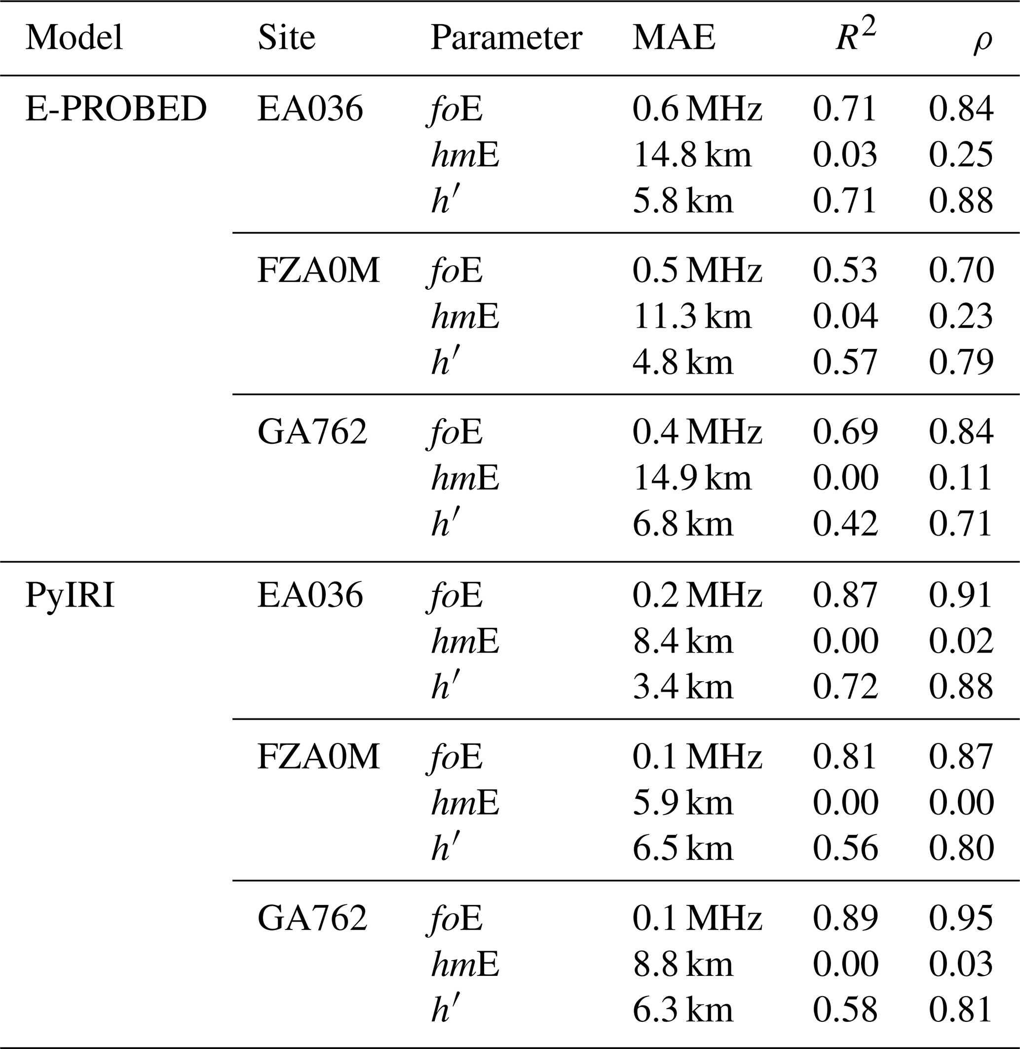
For hmE, the PyIRI constant hmE estimate of 110 km results in lower MAE values than the variable hmE predictions from E-PROBED. However, the resulting R² and Spearman rank-order correlation coefficients (ρ) for PyIRI's hmE predictions are essentially zero, while ρ for E-PROBED hmE ranges from 0.11-0.25. The constant daytime hmE of 110 km in PyIRI originates from IRI's constant value of 105 km that was changed to “110 km based on input from ionosonde and ISR observations” (Bilitza et al., 2022). As suggested by Titheridge (2000), these “reflect the uncertainty caused by a lack of good observational data,” where good ionograms before the year 2000 could only be scaled with a virtual height accuracy of 2–3 km. Even the modern Digisonde 4D has a range resolution of 2.5 km (Galkin et al., 2009). However, as developed by Ivanov-Kholodny et al. (1998) from ISR observations and Titheridge (2000) from ionosondes, time-varying hmE models are currently available showing hmE variations between 105–120 km, which may be beneficial for implementation in IRI/PyIRI.

The large difference between auto-scaled and manually-scaled hmE estimates as observed in Fig. A3 must be taken into account to fully understand the uncertainties involved with auto-scaled ionogram parameters. The manually-scaled hmE estimates over EA036 are nearly 15 km above the auto-scaled values for the same conditions, closely matching the E-PROBED hmE estimates. ARTIST-5 auto-scaling uncertainties have been analyzed in detail by Stankov et al. (2023) for the Dourbes, Belgium Digisonde during 2011–2017, resulting in foE error bounds (auto-scaled value minus manually-scaled value) of [−0.30,0.80] MHz and minimum virtual height of the E region, h^′E, error bounds of [−6,6] km. While the modeled foE values fall within the auto-scaled ionogram uncertainties for foE, the auto-scaled h^′E uncertainties are rather low compared to the models' hmE MAE between 6–15 km. However, the auto-scaled h^′E error bounds during low solar activity show a large underestimation bias for the auto-scaled estimates ranging from [−15.0,2.5] km (Stankov et al., 2023). The -15 km error bound matches the 15 km hmE underestimation observed during the 2009 solar minimum over EA036, indicating that the large errors in E-PROBED hmE estimates during solar minimum may simply be an artifact of auto-scaled errors. As the auto-scaled error bounds are reduced during solar maximum, the E-PROBED hmE estimates are overestimated during these times. The general trend of underestimated peak height altitudes from ARTIST-5 auto-scaled ionograms was also observed for hmF2 when compared against GNSS-RO and ISR estimates (Swarnalingam et al., 2023), and the hmE differences between auto- and manual-scaled ionograms observed in Figs. A3–A4 suggest that perhaps an offset could be calculated to correct the auto-scaled estimates. However, this offset would likely depend on several factors such as solar cycle and ionosonde site (hardware, climatology, etc.), requiring a significant effort to obtain appropriate correction factors. Ideally, a future study with a larger collection of manually-scaled ionograms spanning several years could be used to reanalyze the models' hmE predictions and remove the inconsistencies stemming from auto-scaling.

It must also be noted that hmE is dependent on a parabolic fit to the E region virtual height observations (Reinisch and Xueqin, 1983; Titheridge, 1985a), which means that the scaling errors for h^′E and errors in hmE are not expected to be one-to-one. However, differences in the starting altitude of virtual height observations will certainly impact the hmE estimates, and the differences between manually-scaled and auto-scaled hmE observations align well with the expected errors in h^′E. An additional uncertainty/error within ionogram-derived hmE estimates is caused by the assumed parabolic layer shape for the E region that approaches a zero plasma frequency at the bottom of the E region rather than smoothly transition to the nonzero D region densities. As discussed in detail in Shaver et al. (2023), the lack of a D to E region transition during ARTIST-5 ionogram inversion along with a required parabolic profile fit (that can introduce exaggerated $\mathrm{d}z/\mathrm{d}{f}_{\mathrm{p}}$ near foE) may result in a small bias for the bottom of the parabolic layer on the order of a few kilometers.

Compared with previous comparisons of E region models with ionosonde observations, the results generally align with the present study. Mikhailov et al. (1999) found similar seasonal trends with the El Arenosillo Digisonde throughout 1995. They also found relatively close agreement with IRI's foE estimates and ionosonde observations, but noted that a chemistry-based model could reproduce the hmE variations not captured by IRI. The foE and hmE model developed by Titheridge (2000) was able to reduce hmE errors to less than 5 km and foE errors below 0.1 MHz when compared to manually-scaled ionograms from Auckland, New Zealand, which is a significant reduction from the hmE errors observed here for E-PROBED and PyIRI. Yue et al. (2006) found that IRI overestimated foE over Wuhan, China, especially between May and September. Pavlov and Pavlova (2013) developed a photochemistry-based NmE model that showed reasonable agreement with an ionosonde at Boulder, Colorado for low solar activity, but required a factor of 2 increase in the 3.2–7.0 nm flux from EUVAC to match observations during high solar activity. A comparison of IRI foE predictions with an ionosonde at Chumphon Station, Thailand, found the largest differences during sunrise and sunset, but very low overall errors (Wongcharoen et al., 2015). Mostafa et al. (2018) also found a slight overprediction by IRI compared to manually-scaled ionograms from the Nicosia, Cyprus Digisonde. For hmE, they observed similar diurnal and seasonal trends, although their manually-scaled ionograms provided hmE values below IRI's constant value of 110 km. Further, they conclude that large differences between IRI and the ionosonde observations may be due to non-Chapman like behavior of the E layer, which was also noted by Ivanov-Kholodny et al. (1998). These results are consistent with the auto-scaled ionograms shown here, although our manually-scaled ionograms from EA036 show elevated hmE values above 110 km.

In contrast to foE and hmE estimates from ionogram inversions, virtual heights are directly measured by ionosondes, making them a useful tool for model validation. The virtual height (h^′) for a particular transmit frequency (f) is defined as the integral of the group index of refraction as a function of altitude, which may also be represented as the group index (μ^′) as a function of frequency times the gradient of the real-height with respect to frequency:

$$\begin{array}{}\text{(1)}& {\displaystyle }{h}^{\prime }\left(f\right)& {\displaystyle }=\underset{\mathrm{0}}{\overset{f}{\int }}{\mathit{\mu }}^{\prime }(f,f_{\mathrm{p}}){\displaystyle \frac{\mathrm{d}z}{\mathrm{d}{f}_{\mathrm{p}}}}\mathrm{d}{f}_{\mathrm{p}},\text{(2)}& {\displaystyle }{\mathit{\mu }}^{\prime }& {\displaystyle }={\left(\mathrm{1}-{\displaystyle \frac{f_{\mathrm{p}}^{\mathrm{2}}}{f^{\mathrm{2}}}}\right)}^{-\mathrm{1}/\mathrm{2}},\end{array}$$

where f_p is the plasma frequency (Budden, 1966). Equation (2) is a simplified form of the group index of refraction for an unmagnetized, collisionless plasma, and is shown here instead of the full form for an O-mode to show the basic relationship with respect to the plasma frequency. This dependence on f_p and $\mathrm{d}z/\mathrm{d}{f}_{\mathrm{p}}$ provides a method for analyzing modeled E region shapes and gradients that is free from uncertainties produced by profile shape assumptions used during ionogram inversion. However, due to the integrated nature of the virtual heights, it is possible to produce the same virtual heights from various EDPs, meaning that virtual height agreement does not necessarily indicate agreement on profile shapes overall. Although a direct comparison with ionosonde-derived EDPs may seem like a more straightforward approach, the various assumptions required for ionogram inversion result in a final product that is no longer a direct measurement (see the discussion in Shaver et al., 2023).

For the sites analyzed here, both PyIRI and E-PROBED showed reasonable agreement with the measured virtual heights with MAE ranging from 5–7 km for E-PROBED and 3–7 km for PyIRI (Table 1). Although similar performance for both models may appear to indicate similar profiles that agree with ionosonde observations, the differences in predicted foE and hmE prove that this is not the case. Even with differing EDPs, the altitude integrals of the group indices derived from the EDPs result in similar virtual heights that generally agree with ionosonde observations. Although, a bias exists for each site: the models tend to underestimate the virtual heights for EA036, while the models tend to overestimate the virtual heights for FZA0M and GA762. Since the EA036 period of comparison for virtual heights was January–March 2009 (solar minimum) and was mostly composed of manually-scaled ionograms while FZA0M and GA762 consisted of auto-scaled ionograms, the change in bias from underestimation to overestimation is likely an artifact of ARTIST-5 autoscaled uncertainties for h^′E (Stankov et al., 2023). Even here, where we assume that the virtual heights are direct measurements to be used as ground-truth, an uncertainty exists from auto-scaling that must be considered when interpreting the accuracy of the modeled virtual heights.

5 Conclusions

A comparison of E region predictions from E-PROBED, PyIRI and ionosondes was performed for three sites: mid-latitude El Arenosillo, Spain (EA036), low-latitude Fortaleza, Brazil (FZA0M), and high-latitude Gakona, Alaska (GA762). Manually-scaled or auto-scaled ionograms using ARTIST-5 were used as the ground-truth for foE and hmE estimates, and both models were run for each ionogram time spanning from 2009–2024 for EA036 and GA762, and 2015–2024 for FZA0M. Additionally, a subset of ionograms were used to compare against modeled virtual heights calculated from the models using a numerical ray tracer.

The key results of the comparison are listed below:

• Overall, both E-PROBED and PyIRI showed reasonable agreement with the ionosonde observations, properly capturing the foE solar cycle, seasonal, and diurnal trends.

• For foE, the E-PROBED estimates were generally larger than the PyIRI estimates, which were slightly larger but nearly equal to the ionosonde observations. Mean Relative Absolute Errors (MRAEs) peaked around 70 % for E-PROBED at dusk, while PyIRI produced lower MRAE peaks around 10 % for times ranging from late morning to dusk.

• For hmE, both models showed weaker agreement with auto-scaled ionograms; E-PROBED overestimated by ∼15 km and PyIRI predicted a constant hmE of 110 km. The large bias in E-PROBED hmE estimates almost disappears when compared to manually-scaled ionograms, indicating that great care must be taken when comparing against auto-scaled hmE estimates.

• Modeled virtual heights derived from E-PROBED and PyIRI showed reasonable agreement with measured virtual heights overall. Since ionosondes measure virtual heights directly, this comparison provides confidence in the integrated electron density profiles as a function of altitude. A slight bias exists in the modeled virtual heights that reverses direction for manual- versus auto-scaled ionograms, indicating that auto-scaled uncertainties are also present in the virtual height observations, similar to hmE.

This comparison provides confidence in the use of E-PROBED and PyIRI for global E region predictions. While both models can be improved in future iterations, the solar cycle, seasonal, and diurnal trends were captured well overall. A similar study using only manually-scaled ionograms for E region observations would be helpful, especially given the large ambiguities arising from differences in the manually-scaled and auto-scaled ionogram estimates of hmE.

Appendix A: Seasonal and Diurnal Results

A1 EA036

Seasonal foE trends are displayed in Fig. A1 with monthly quartiles. While the manually-scaled foE values show a lower maximum than the auto-scaled results, it must be noted that a variety of solar cycle conditions are shown here and the auto-scaled ionograms are constrained to 2009. A seasonal variation is readily observed with foE peaks in local summer and troughs in local winter. Median ionosonde observations range from 2.7 MHz in the winter to 3.2 MHz in the summer. Similarly, PyIRI median foE values range from 2.7–3.4 MHz, and E-PROBED ranges from 3.1–4.0 MHz. The same seasonal trends are observed between the models and ionosonde observations, with a slight foE overestimation from E-PROBED.

Diurnal foE trends are shown in Fig. A2. As expected, the foE peaks in the early afternoon following the peak in solar Extreme Ultraviolet (EUV) flux, with minima observed near dawn/dusk. Median ionosonde foE measurements range from 1.9 MHz at dawn/dusk to 3.2 MHz in the early afternoon. A slow increase is observed until 08:00 solar local, when the foE increases more rapidly towards the peak. This general trend is also predicted by PyIRI and E-PROBED. PyIRI medians range from 1.9–3.4 MHz, while E-PROBED slightly overestimates with a range of 2.4–3.9 MHz. Interestingly, E-PROBED show an evening minima around 17:00 solar local, followed by a slow foE increase later in the evening.

The seasonal hmE trends from ionosondes show a slight decrease during local summer when the foE values peak (Fig. A3), as expected for a Chapman layer. However, this decrease is relatively small, with median values ranging from 103 km in winter to 100 km in summer. E-PROBED also shows slight seasonal variation with hmE peaks during winter and summer. The medians range from 115–117 km, with a larger spread in predictions during the local summer. E-PROBED hmE predictions generally align with the manually-scaled ionograms, which are nearly 15 km above the auto-scaled values.

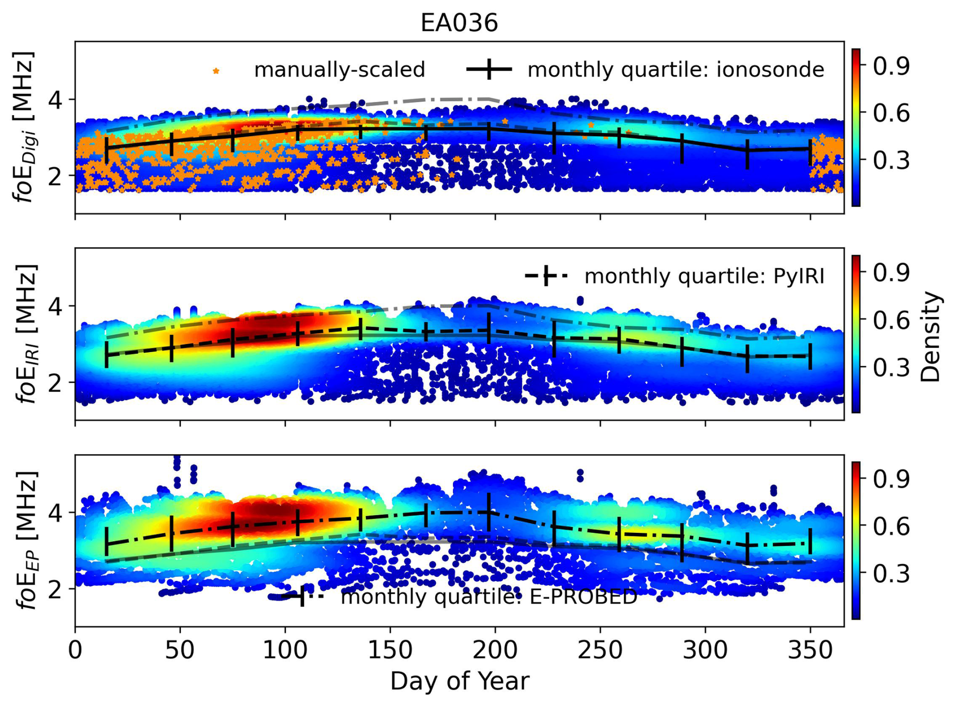
Figure A1 Day of Year foE estimates for El Arenosillo using ionograms (top), PyIRI (middle), and E-PROBED (bottom). Black trend lines intersect the monthly medians, with quartiles (25 % and 75 %) shown as error bars. For comparison, semi-transparent lines show the median trends for the other two datasets.

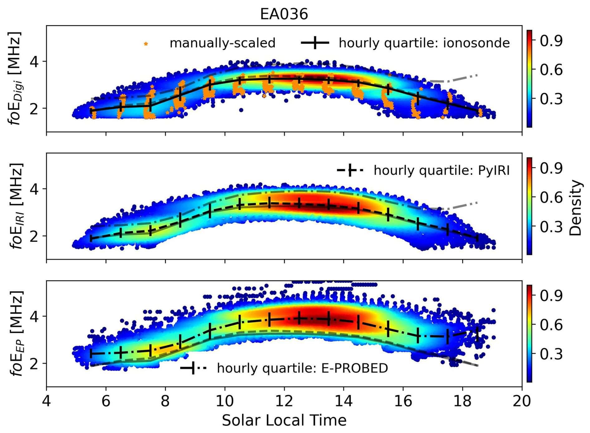
Figure A2 Solar local time foE estimates for El Arenosillo using ionograms (top), PyIRI (middle), and E-PROBED (bottom). Black trend lines intersect the hourly medians, with quartiles (25 % and 75 %) shown as error bars. For comparison, semi-transparent lines show the median trends for the other two datasets.

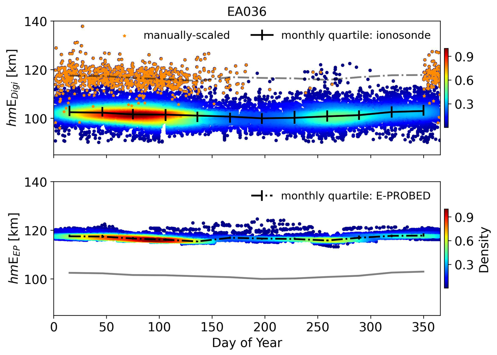
Figure A3 Day of Year hmE estimates for El Arenosillo using ionograms (top) and E-PROBED (bottom). Black trend lines intersect the monthly medians, with quartiles (25 % and 75 %) shown as error bars. For comparison, semi-transparent lines show the median trends for the other dataset.

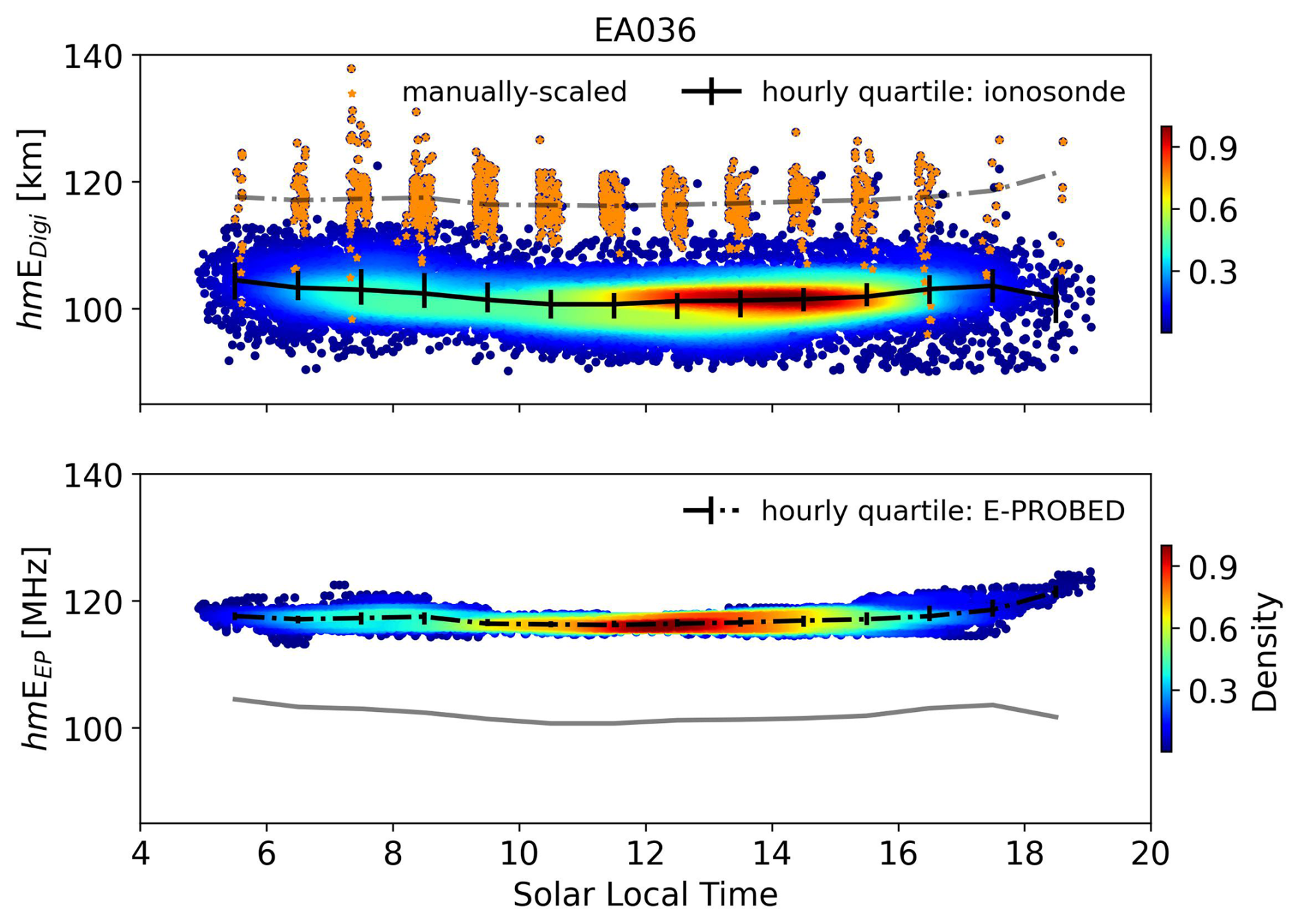
Figure A4 Solar local time hmE estimates for El Arenosillo using ionograms (top) and E-PROBED (bottom). Black trend lines intersect the hourly medians, with quartiles (25 % and 75 %) shown as error bars. For comparison, semi-transparent lines show the median trends for the other dataset.

Solar local time hmE variations (Fig. A4) show minima near local noon and slight increases toward dusk/dawn. Similar to the seasonal trends, the diurnal changes are relatively small (2–3 km) for both ionosondes and E-PROBED with general agreement on the altitudes for the manually-scaled ionograms.

A2 FZA0M

The seasonal trends are less pronounced for this equatorial site compared to the mid-latitude EA036, and both models agree with the relatively small seasonal variations from ionosonde observations (Fig. A5). E-PROBED shows the largest range of predictions throughout day of year, although the variation does not appear to follow a seasonal trend. The ionosonde and PyIRI foE estimates are generally constant throughout the year.

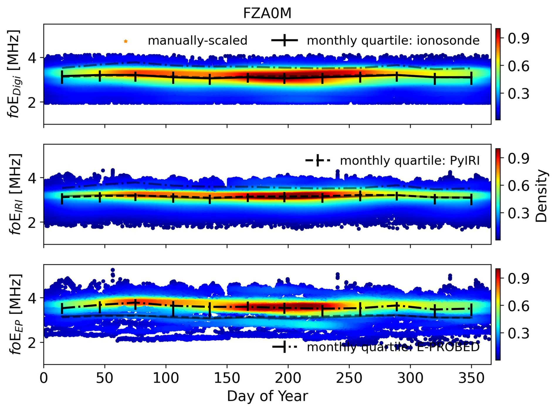
Figure A5 Day of Year foE estimates for Fortaleza using ionograms (top), PyIRI (middle), and E-PROBED (bottom). Black trend lines intersect the monthly medians, with quartiles (25 % and 75 %) shown as error bars. For comparison, semi-transparent lines show the median trends for the other two datasets.

For the diurnal variation, the ionosonde and PyIRI estimates show a strong symmetry around local noon (Fig. A6). In contrast, E-PROBED predicts a dawn-dusk asymmetry with a dawn median of 2.4 MHz and a dusk median of 3.1 MHz.

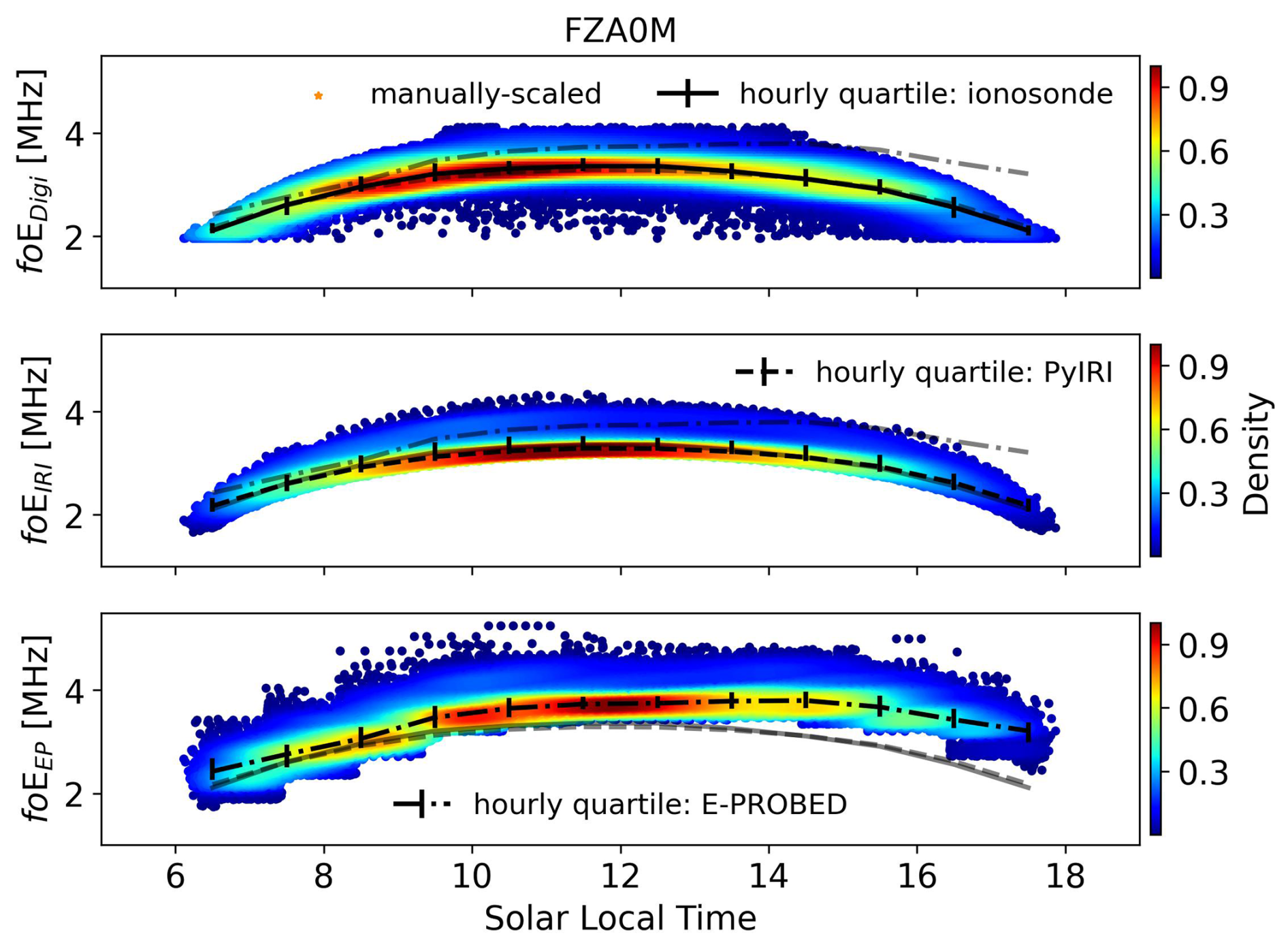
Figure A6 Solar local time foE estimates for Fortaleza using ionograms (top), PyIRI (middle), and E-PROBED (bottom). Black trend lines intersect the hourly medians, with quartiles (25 % and 75 %) shown as error bars. For comparison, semi-transparent lines show the median trends for the other two datasets.

Solar cycle hmE trends for Fortaleza are displayed in Fig. A7, showing the expected increase in altitude during solar minimum when the foE values are reduced. Similar to the EA036 auto-scaled ionogram observations, median hmE altitudes are below ∼105 km with a range of 90–120 km, while PyIRI predicts a constant hmE of 110 km and E-PROBED predicts median values around 115 km with a reduced range.

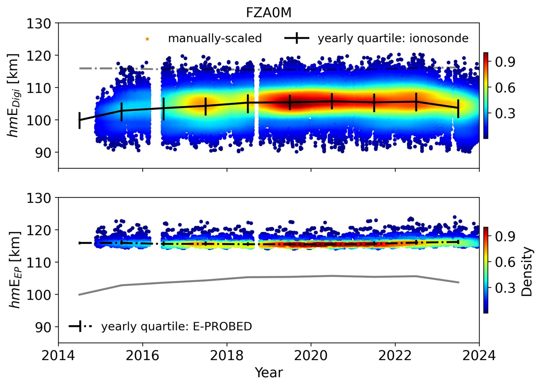
Figure A7 Yearly hmE estimates for Fortaleza using ionograms (top), and E-PROBED (bottom). Black trend lines intersect the yearly medians, with quartiles (25 % and 75 %) shown as error bars. For comparison, semi-transparent lines show the median trends for the other dataset.

A3 GA762

Seasonal trends are similar between both models and the ionosonde observations (Fig. A8), with a slight flattening toward local winter observed in the E-PROBED trends. The diurnal variation is less pronounced at this high-latitude site, but foE peaks are still observed near local noon (Fig. A9). Of note, both PyIRI and the ionosonde estimates show a double peak in data density near local noon (two distinct foE peaks), while E-PROBED has a single peak. This double peak in data density may be due to seasonal variations, where PyIRI and ionosondes have a higher data density at elevated foE near the local summer, while the summer E-PROBED estimates are relatively low compared to the winter values (Fig. A8).

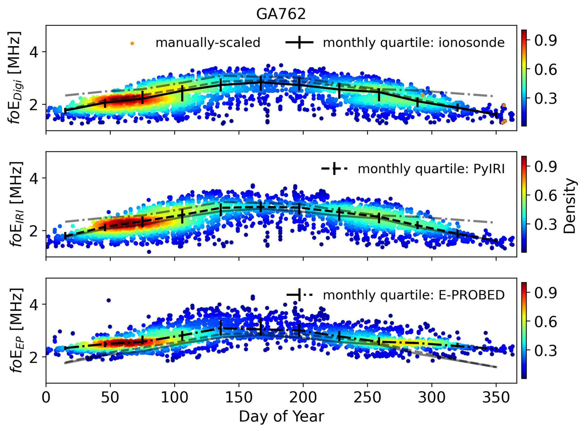
Figure A8 Day of Year foE estimates for Gakona using ionograms (top), PyIRI (middle), and E-PROBED (bottom). Black trend lines intersect the monthly medians, with quartiles (25 % and 75 %) shown as error bars. For comparison, semi-transparent lines show the median trends for the other two datasets.

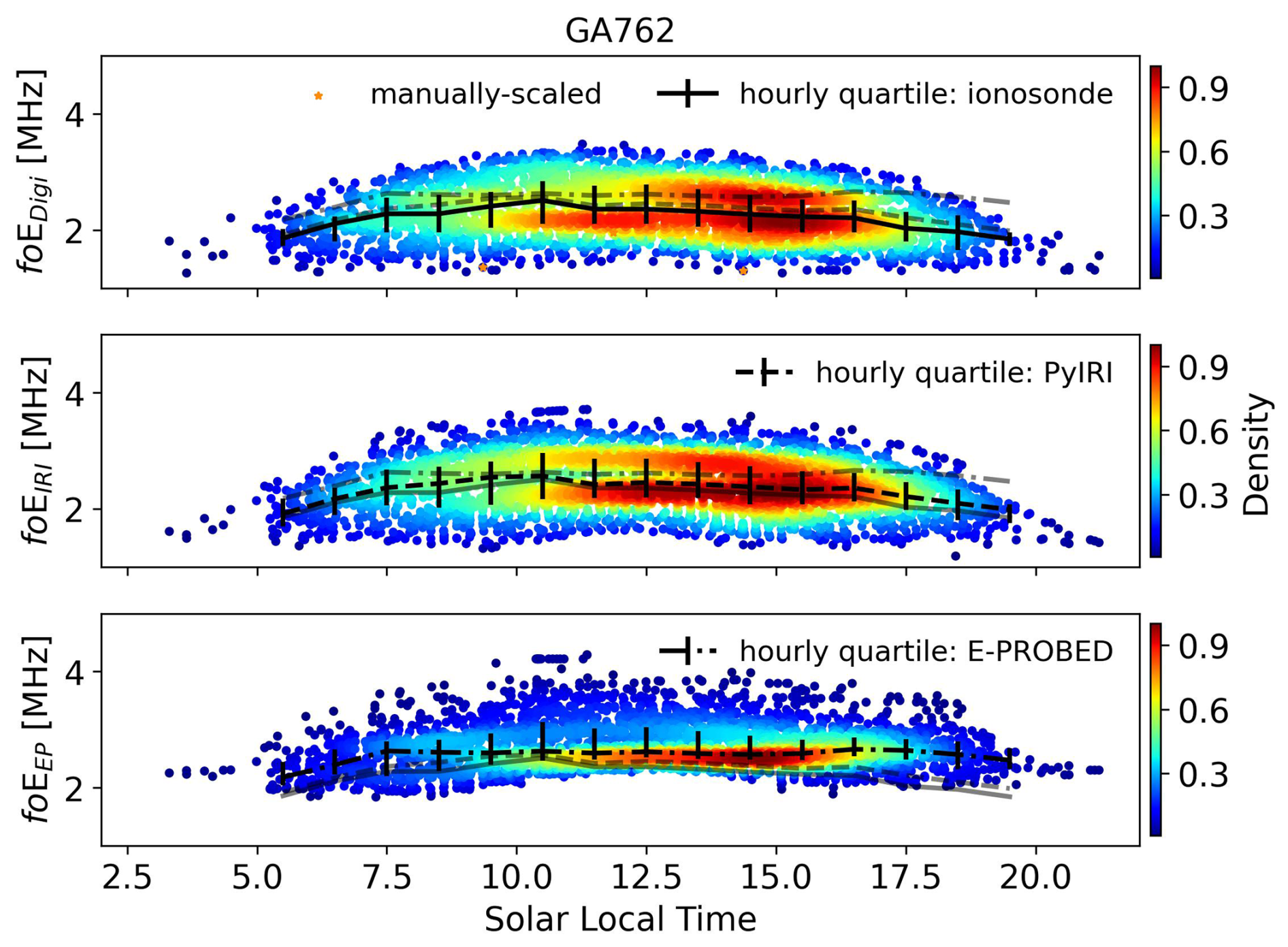
Figure A9 Solar local time foE estimates for Gakona using ionograms (top), PyIRI (middle), and E-PROBED (bottom). Black trend lines intersect the hourly medians, with quartiles (25 % and 75 %) shown as error bars. For comparison, semi-transparent lines show the median trends for the other two datasets.

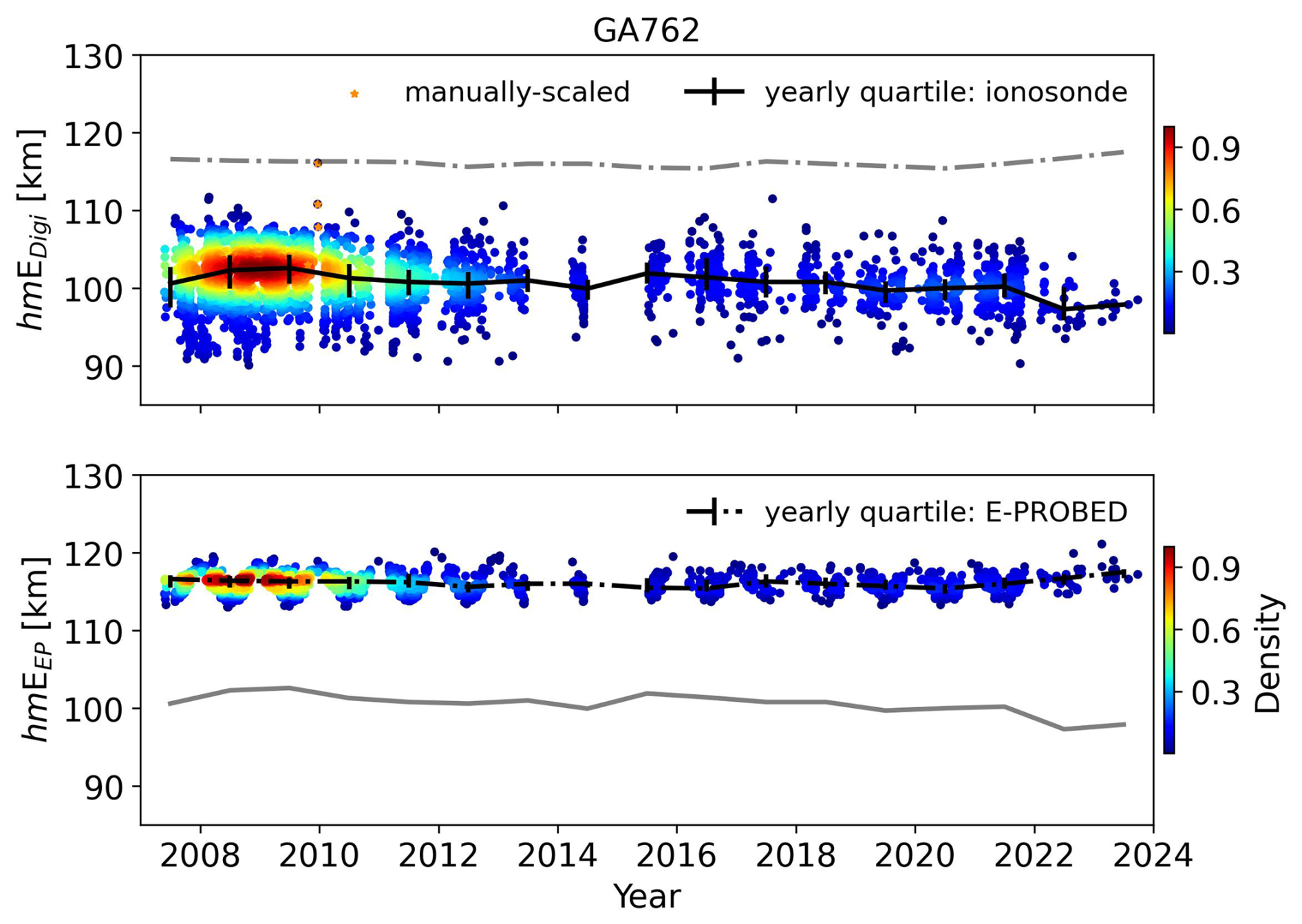
Figure A10 Yearly hmE estimates for Gakona using ionograms (top) and E-PROBED (bottom). Black trend lines intersect the yearly medians, with quartiles (25 % and 75 %) shown as error bars. For comparison, semi-transparent lines show the median trends for the other dataset.

The hmE trends for GA762 are similar to EA036 and FZA0M with E-PROBED estimates larger than PyIRI (which are held at a constant 110 km), which is greater than the auto-scaled ionogram estimates (Fig. A10). Subtle solar cycle variations are present in the ionosonde data with slight decreases in altitude during solar maximum, but these subtle variations are not observed in the model predictions. Interestingly, the few manually-scaled ionograms show a trend similar to that of EA036 where the hmE values are much larger than the auto-scaled values.