Juice/SWI during the Lunar-Earth-Gravity-Assist (LEGA) – Part 4: Antenna pointing and beam characterisation

The Submillimetre Wave Instrument (SWI) onboard the Jupiter Icy Moons Explorer (Juice) spacecraft consists of a 29 cm off-axis paraboloid antenna and two double-sideband heterodyne receivers operating in the frequency ranges of 530–638 and 1066–1286 GHz. This instrument is designed to study Jupiter's atmosphere and the exospheres of the Galilean moons. We used the Lunar-Earth-Gravity-Assist (LEGA) data from August 2024 to characterise this antenna using several SWI observations pointing towards the Earth. The data analysis of the LEGA observations dedicated to the antenna beam allows us to characterise the antenna beam Full Width at Half Maximum (FWHM), sidelobes, absolute pointing and receiver coalignement. Moreover, an estimate of the calibration efficiency factor has been obtained from an optical model simulation.

1 Introduction

The Juice mission (JUpiter ICy moon Explorer, Grasset et al., 2013) is an ESA Large-class mission selected during cosmic-vision 2015–2025 program. The spacecraft was launched on 14 April 2023 from Kourou, French Guiana by an Ariane 5 launcher, and is scheduled to arrive at Jupiter in July 2031. To achieve its scientific objectives, Juice will first orbit Jupiter and perform several flybys of the Galilean moons before performing an orbital insertion around Ganymede in December 2034. A payload with more than 10 scientific instruments onboard the spacecraft will be used to study the Jupiter system and their moons. Among these instruments, the Submillimetre Wave Instrument (SWI, Hartogh et al., 2026) is a single-pixel heterodyne receiver that operates in the sub-millimetre wavelength range with two tunable frequency channels at 530–638 GHz (CH1) and 1066–1286 GHz (CH2). In its frequency range, SWI's spectrometers observe continuum emission as well as rotational lines of abundant molecules at high spectral resolution. This will enable the characterisation of winds, temperatures, and the chemical composition of the atmospheres and exospheres in the Jovian system. For the moons of Jupiter, SWI will also provide new clues on the contribution of volcanic and sublimation sources (at Io) and the interaction of exospheres with the Jovian magnetosphere. During the Juice mission, the first Lunar and Earth Gravity Assist (LEGA) maneuver took place in August 2024. The SWI team took this opportunity to conduct numerous observations to characterise the various observation modes. Cavalié et al. (2026) described in detail the observation geometry during the LEGA maneuver, the observation planning methodology, the observation modes (e.g. 1D scan and 2D map), and the complete list of the SWI planned and executed observations, listed in order of their unique Observation Identifier numbers (ObsIDs).

This paper is structured as follows. Section 2 briefly describes the instrument. Section 3 presents the analysis of LEGA observations of the Earth and their implications for instrument characterisation, including main beam width measurements (Sect. 3.1). The antenna pointing and receiver coalignment between the Continuum Channels 1 (CCH1) and 2 (CCH2) is described in Sect. 3.2. Section 4 discusses the antenna beam sidelobes and their comparison with the simulated beam, and Sect. 4.1 provides an estimate of the antenna calibration efficiency factor.

2 Instrument description

The instrument consists of a Cassegrain telescope with a 29 cm off-axis antenna and an active pointing mechanism, allowing the dish to be pointed Along Track (AT) and Cross Track (CT) with an angular throw of ±72.5 and ±4.3°, respectively. The antenna dish is mounted atop the receiver unit. Furthermore, SWI has a radiator unit to dissipate heat and two electronic units (Hartogh et al., 2026). Those contain the Chirp Transform Spectrometer (CTS) and the Auto Correlator Spectrometer (ACS), with bandwidths of 1 and 4.4 GHz, and with a spectral resolution of 0.1 and 4.3 MHz, respectively. Jarchow et al. (2026) describe these backends in detail, along with the flux calibration method of the SWI's continuum and spectral line. Before reaching the two receivers, the beam is split using a polarising wire-grid. This implies that each band is observed in a single polarization. The two heterodyne receivers can be tuned in the frequency ranges of 530–638 and 1066–1286 GHz, respectively. The receiver's detection stage is a mixer that uses GaAs Schottky diode technology. The incoming sky signal is mixed with a tunable local oscillator signal (the LO frequency) near 600 and 1200 GHz, which is provided by a tunable microwave synthesizer phase locked to an Ultra-Stable Oscillator (USO) at 80 MHz. Consequently, this heterodyne principle technique converts the sky frequency to a lower frequency, centered at the Intermediate Frequency (IF) of 6.0 GHz. At the IF, the signal can be amplified and routed to a spectrometer. The receivers operate in Double Side-Band (DSB) mode which results in both the Upper Side-Band (USB) and the Lower Side-Band (LSB) on both sides of the LO frequency being detected simultaneously. Additionally, the Continuum Channel (CCH) can be recorded simultaneously during CTS measurements, containing an integrated value over a bandwidth of 4 GHz. Consequently, if the continuum value is of interest, CCH often allows for a higher signal–to–noise ratio.

3 Beam parameters

As with any telescope, the antenna of SWI convolves the observed signal with its point spread function. In radio astronomy, it is often referred to as the antenna beam pattern, and it is typically described as consisting of a main beam and sidelobes. The beam width of a circular antenna of diameter D is typically close to the diffraction-limit ($\mathrm{1.22}\mathit{\lambda }/D$). In this section we focus on the main beam, determining its Full Width at Half Maximum (FWHM), ellipticity and the pointing accuracy from several observing modes. This allows us to verify our methodology and to assess the suitability of the available observing modes to constrain relevant parameters.

3.1 Main beam width

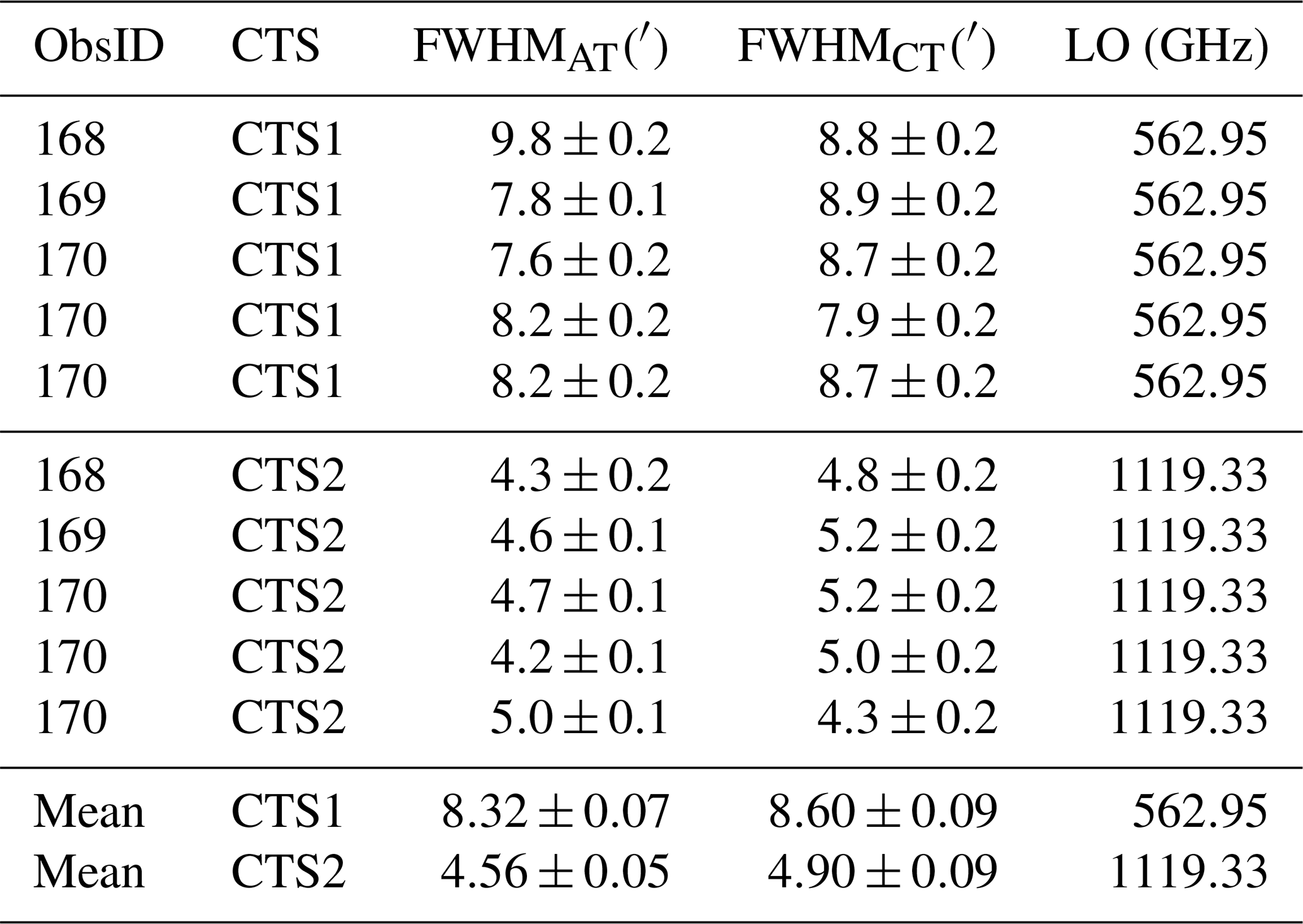
The simplest approach characterising the main beam involves analysing observations of a point source, such as an unresolved planet, by the instrument. The intensity measured by the instrument is then a convolution of the beam pattern with the point source, which can be described as a Dirac delta distribution δ. This method was employed on observations made on 8 July 2023 during the Near Earth Commissioning Phase (NECP), when the Earth angular diameter was 2.045 arcmin. The SWI team focused on characterising the AT, CT pointing accuracy using 2D map measurements. The goal was to find the right pointing offset corrections for the AT and CT mechanisms that encapsulates all deviations/errors, (e.g, due to mounting of the base plate, own mechanical end-switches performances, motor step sizes). Furthermore, these 2D map observations also allowed to measure the SWI beam widths for the first time in-flight. The results of this analysis performed by Jarchow and Rezac (2025), are presented in Table 1. The averaged NECP value of the beam ellipticity was equal to 1.03±0.02 and 1.07±0.02 for CTS1 and CTS2, respectively. One of the goals of this work is to compare these values with our analysis performed on more recent observations from LEGA. This will allow us to better describe the instrument performance and possibly its evolution over time.

Table 1 Observed main beam FWHM along AT and CT from NECP adapted from Jarchow and Rezac (2025). The LO frequencies of these observations are fixed and used as reference LO frequencies – allowing comparison between observations with different tunings. Since ObsID 170 contains several maps, multiple beam width measurements were obtained. In this work we compute weighted means and their uncertainties using the method of propagation of errors.

Another method for determining the beam characteristics involves analysing scans that cross the limb of targets that are much larger than the main beam. This approach was previously used by Greve et al. (1998), Baars and Kärcher (2018), Tercero et al. (2021). The beam profile can be retrieved from the sharp edge of a resolved source such as Earth. In practice, the observed signal corresponds to a convolution of the antenna beam with the target brightness distribution. If the angular size of the target is sufficiently large, we can consider the resulting signal as a convolution of the beam pattern g(x) and a Heaviside function H(x) representing the target. By differentiating this convolution, we obtain the beam pattern centred at the planet edge:

$$\begin{array}{}\text{(1)}& \begin{array}{rl}{\displaystyle \frac{\mathrm{d}}{\mathrm{d}x}}(H*g)\left(x\right)& =\left({\displaystyle \frac{\mathrm{d}H}{\mathrm{d}x}}*g\right)\left(x\right)\\ & =({\mathit{\delta }}_{\mathrm{edge}}*g)\left(x\right)=g(x-x_{\mathrm{edge}}),\end{array}\end{array}$$

with δ_edge the Dirac delta distribution located at the planet edge position x_edge, which gives us the beam pattern centered at the target limb. Consequently, we can fit the full beam pattern, including the beam and side lobes. Using a simple Gaussian model meant to represent only the main beam:

$$\begin{array}{}\text{(2)}& g(x;\mathit{\mu },\mathit{\sigma })={\displaystyle \frac{\mathrm{1}}{\sqrt{\mathrm{2}\mathit{\pi }}\mathit{\sigma }}}\exp \left(-{\displaystyle \frac{(x-\mathit{\mu }{)}^{\mathrm{2}}}{\mathrm{2}{\mathit{\sigma }}^{\mathrm{2}}}}\right),\end{array}$$

we obtain the position of the target limb μ and the beam FWHM as $\mathrm{2}\sqrt{\mathrm{2}\ln \left(\mathrm{2}\right)}\mathit{\sigma }$. Since fitting the main beam only requires a Gaussian model, we can skip differentiating the signal entirely. Instead, we can integrate the main beam model (Eq. 2) and use an error function:

$$\begin{array}{}\text{(3)}& \mathrm{erf}(x;\mathit{\mu },\mathit{\sigma })=\underset{-\mathrm{\infty }}{\overset{x}{\int }}g(x^{\prime };\mathit{\mu },\mathit{\sigma })\mathrm{d}{x}^{\prime },\end{array}$$

to fit the data directly yielding the same model parameters μ and σ. This fitting method avoids the problems associated with the differentiation of a noisy signal, resulting in a robust approach, applicable to several observing modes (Formánek and Moreno, 2025). Furthermore, depending on the geometry of the observations, we will determine the FWHM along the pointing directions AT and CT (1D scans) or under the assumption of radial symmetry (2D maps).

In the following sections, since the frequency ν varies between observations, the measured beam FWHM(ν) is scaled to a reference beam: FWHM_Scaled(ν_r), at the reference frequencies ν_r of 562.95 and 1119.33 GHz for the two channels, respectively; following the diffraction-limit law as:

$$\begin{array}{}\text{(4)}& {\mathrm{FWHM}}_{\mathrm{Scaled}}\left({\mathit{\nu }}_{\mathrm{r}}\right)=\mathrm{FWHM}\left(\mathit{\nu }\right)\times \mathit{\nu }/{\mathit{\nu }}_{\mathrm{r}}.\end{array}$$

In the next subsections we present an analysis of the data from SWI 1D scans and 2D map observations performed during the LEGA flybys in August 2024. These values will provide a comparison to the parameters determined earlier during NECP and listed in Table 1.

3.1.1 1D Scan observations

Following the LEGA flybys, several 1D scans of Earth were obtained by SWI. These observations contain 1D scans of the target (the Earth in this case) along the orthogonal AT or CT axes and were measured in pairs. Figure 1 shows an example of a 1D scan observation, along with the fits obtained using the method described in the previous section. As described in more detail in Tables A1 and A2, we have two pairs of observations scanning back and forth, with a sampling range from 2^′ to 6^′, which allow for a good estimate of the FWHM. Furthermore, comparing the ratios of FWHM_AT $/$ FWHM_CT for each pair allows us to assess the ellipticity of the beam. Variations in the continuum of approximately 5 % to 10 % are observed, primarily in the inner part of the disk along the CT direction, which correspond mainly to spatial variations in latitude (see Fig. 1 the CT images). These variations can also disrupt the transition edge at the limb used for pointing measurements. However, it should be noted that the FWHM measurement depends essentially on the derivative of the continuum at the limb, which is less sensitive to these continuum variations in the inner part of the disk. Nevertheless, in order to minimize sensitivity to these variations, we conducted numerous tests to determine the optimal width to consider for beam fitting at the limb. The best solution found was to consider a width of ±2 half-beams around each limb.

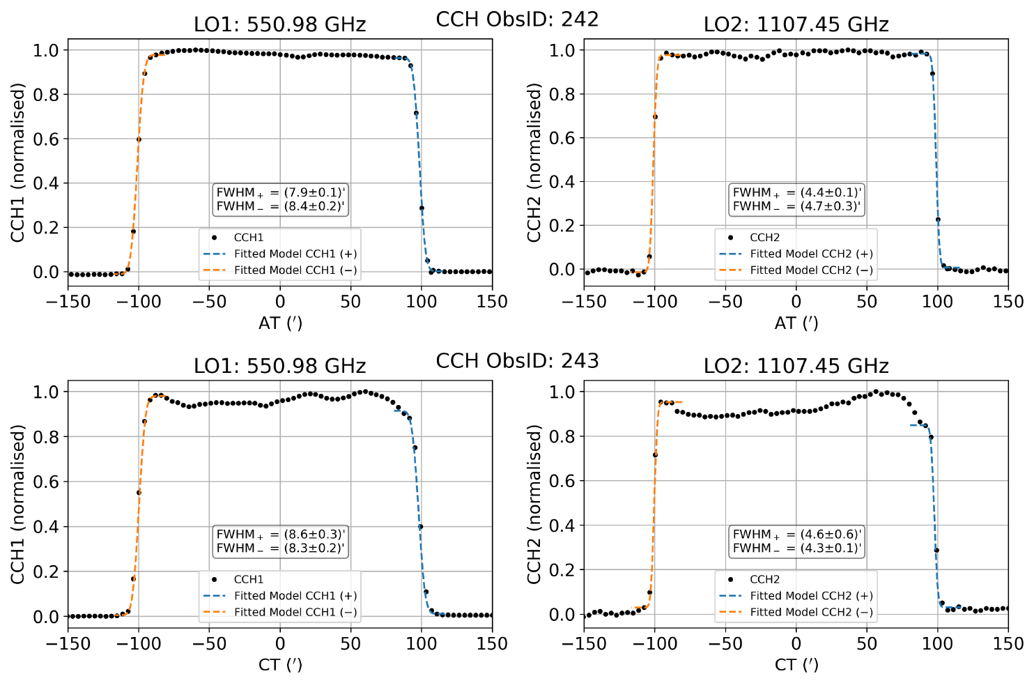
Figure 1 Examples of FWHM fitting from 1D scan data for AT ObsID 242 (top) and CT ObsID 243 (bottom). CCH1 and CCH2 are the continuum channels 1 and 2, respectively.

Table 2 FWHM measurements obtained from 1D scans along AT and CT. The two lines for each measurement correspond to a fit on the right and left limb of the target. The scaled values correspond to reference frequencies of 562.95 and 1119.33 GHz for the two channels, respectively.

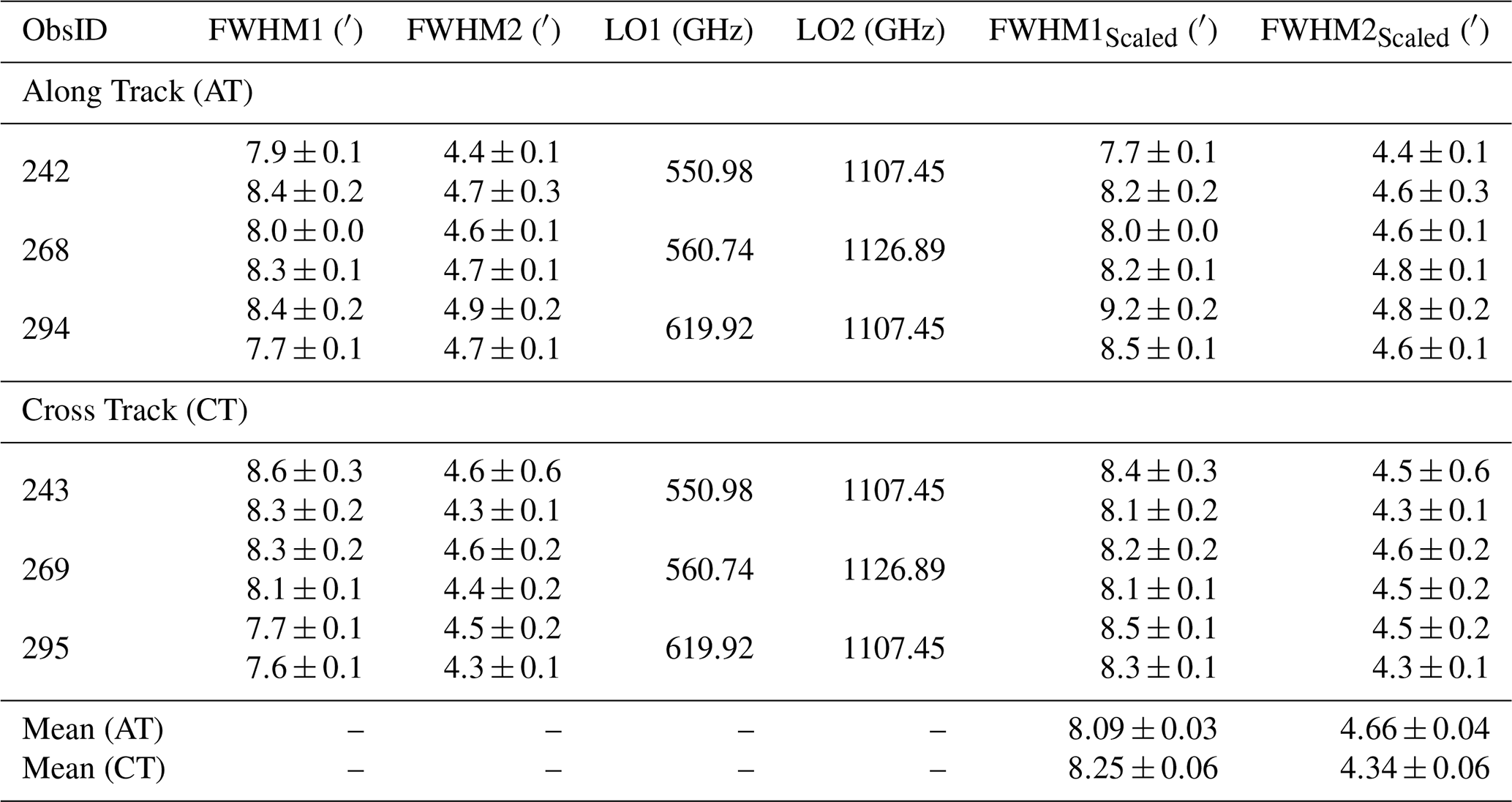
Results of the FWHM fitting can be found in Table 2. We obtain these results by fitting both limbs of the 1D scan with an error function. Additionally, by averaging the individual FWHM_AT $/$ FWHM_CT ratios, we obtain an average value of the beam ellipticity of 1.01±0.02 for channel 1 and 1.06±0.03 for channel 2, both consistent with results obtained during NECP (see Table 1). From this we can conclude that the values of FWHM do not differ significantly along different axes and the beam is mostly circular. This supports that no significant asymmetry is present and validates the use of a radially symmetric beam model in subsequent analysis.

3.1.2 2D Map observations

During the 2D map observations, the instrument follows a pointing pattern shown by Cavalié et al. (2026) in their Fig. B2. After the first flyby of the Earth, SWI performed observations of the Earth disk, obtaining several 2D maps for each channel. During these observations, Earth was at a distance of approximately 6×10⁵ km, yielding an angular size of $\sim {\mathrm{75}}^{\prime }$. Consequently, the target was resolved by the beam. In Sect. 3.1.3 we display the resulting continuum images and fit them with a model (see Eq. 5) in order to estimate the pointing accuracy.

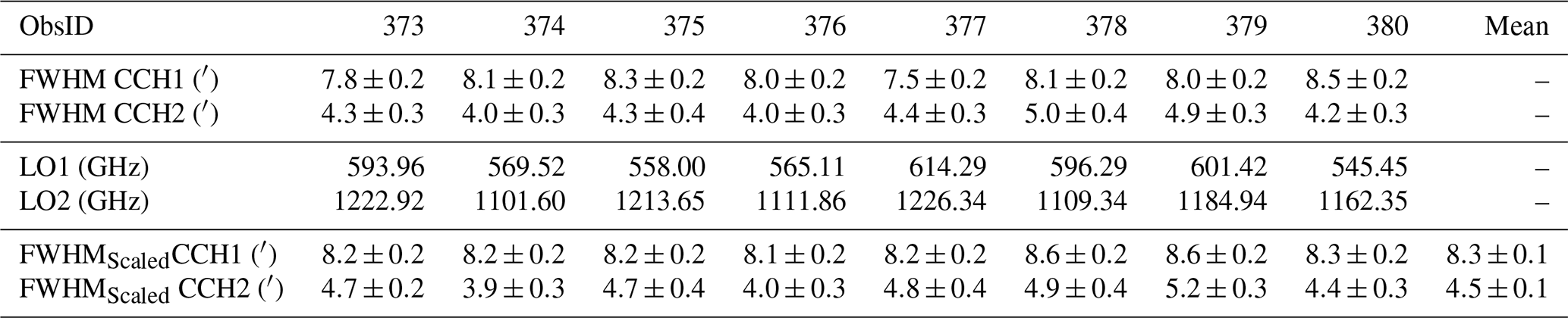
In this subsection, we use the resulting correction of the pointing (see Sect. 3.2) and arrange the measured data as function of the angular separation from the target centre. This way, we create a synthetic limb scan (Fig. 2). In this process we assume a radial symmetry in the target and also a radially symmetric main beam, as we concluded in the previous subsections. These assumptions introduce some noise into the produced synthetic limb scan, mainly because of the variation of intensity across the target disk and the change of its angular size as described in more detail in the following subsection. On the other hand, this effectively increases the sampling Δθ at the limb. We can now apply the same method as previously used during the 1D scans to estimate the size of the main beam. The results of this analysis are provided in Table 3.

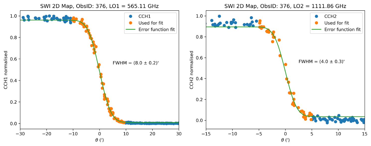
Figure 2 Example of an error function fit applied to a synthetic limb scan, derived from the 2D map ObsID 376. The panels display the Full Width at Half Maximum (FWHM) fits for Continuum Channel 1 (left) and Continuum Channel 2 (right).

Table 3 Main beam parameters determined from 2D map data by fitting an error function under the assumption of radial symmetry. The scaled values correspond to reference frequencies of 562.95 and 1119.33 GHz for the two channels, respectively.

3.1.3 Comparison of methods

By combining the results from NECP with our fitted FWHMs from LEGA (1D scans and 2D maps), we can assess the consistency of our methodology. Figure 3 presents all analysed observations, including several ObsID where the sampling was too sparse (6^′) to constrain the FWHM of channel 2. In addition to the individual values, Fig. 3 reports the scaled weighted mean value (excluding the 1D 6^′ sampling observations) equal to (8.18±0.02) arcmin and (4.60±0.03) arcmin at 562.95 and 1119.33 GHz, respectively. Using only the LEGA data, the retrieved weighted mean FWHM values are (8.13±0.03) arcmin and (4.56±0.03) arcmin. The averaged scaled FWHM values can be found in Table 4. These NECP and LEGA values are in agreement, within the uncertainties, with the ground based near-field measurements (Hartogh et al., 2026), which, when scaled using the reference frequencies, are equal to 8.4 and 4.7 arcmin. In summary, all methods yield consistent FWHM values within uncertainties, confirming both the robustness of the analysis and the stability of the instrument.

Table 4 Average values of the FWHM from NECP, 1D scans, 2D scans and their average. All values have been rescaled to the NECP reference frequencies 562.95 and 1119.33 GHz for the channel 1 and 2, respectively.

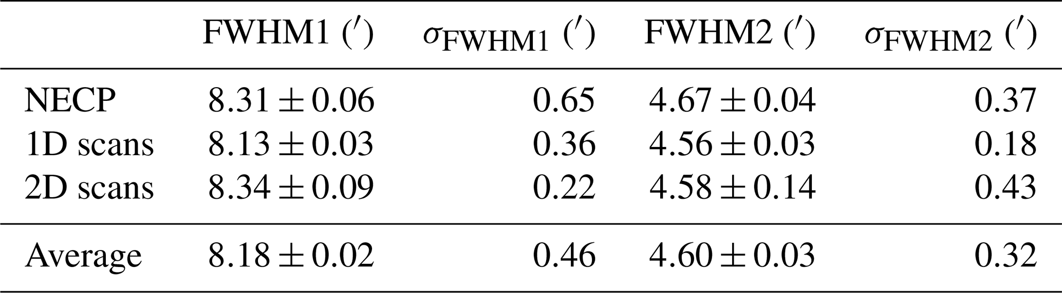
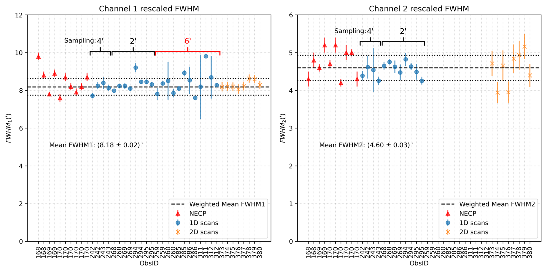
Figure 3 Comparison of scaled FWHM values obtained using different methods. Values are scaled to reference frequencies of 562.95 and 1119.33 GHz, respectively. The red triangles correspond to NECP values adapted from Jarchow and Rezac (2025), while the remaining data points are derived from LEGA data. The two dotted lines surrounding the average represent the standard deviation of individual measurements.

3.2 Pointing offsets

Performing scientific observations most often requires accurate pointing of the instrument. For this reason, the onboard parameters AT₀ and CT₀ serve to compensate any pointing misalignments of the telescope. The pointing offset parameters ΔAT and ΔCT corresponds to the differences between the measured and the commanded target angular positions in AT and CT, respectively, allowing to update the parameters AT₀ and CT₀. They have been determined using broader 2D maps of point-like sources during NECP. However, over time, there might be a shift of a few steps in the motors used to orient the antenna. A single mechanism step along AT or CT corresponds to 29.92^′′ and 8.67^′′, respectively. We use the existing LEGA observations and fit them with a simple model to obtain the pointing offset of the target centre position. Thus, ΔAT and ΔCT offsets that would remain at (0,0) would indicate that the pointing has remained stable and accurately derived since NECP, when AT₀ and CT₀ were first updated. Additionally, since there are two receivers (one for each channel), a slightly different pointing for each channel may occur (coalignement).

Using the 2D maps with 15×15 pixels (for more details see Table A3), we can fit a circular disk function to determine the pointing. We use a tapered circular function defined as

$$\begin{array}{}\text{(5)}& T\left(\text{AT,CT}\right)={\displaystyle \frac{A}{\mathrm{1}+e^{\frac{r-R}{\mathit{ϵ}}}}}\end{array}$$

where $r=\sqrt{(\text{AT}-{\mathrm{\Delta }}_{\mathrm{AT}}{)}^{\mathrm{2}}+(\text{CT}-{\mathrm{\Delta }}_{\mathrm{CT}}{)}^{\mathrm{2}}}$, R is the mean target radius, A is the disk temperature, and ϵ is a small smoothing parameter. We determine the parameters Δ_AT, Δ_CT, R, A and ϵ for the available observations. Performing fits on eight 2D maps measured during LEGA yields results shown in Fig. 4. The resulting fit parameters are listed in Table B1.

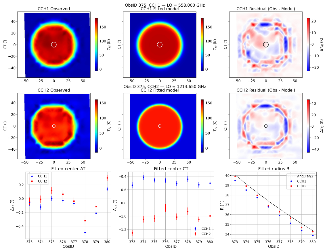
Figure 4 Circular disk fitting for 2D maps of Earth. The first two rows show from left to right the observation, model fit, and the residuals for ObsID 375. The first two rows correspond to the two instrument channels. The last row shows a comparison of selected fit parameters between ObsIDs and in the last panel, the dashed line Angular/2 represents the Earth angular radius at the beginning of the observations. The white circles at the centers represent the beam sizes.

As shown in the last row of Fig. 4, the ΔAT values vary across the observations, with values close to 0^′ in average recorded in both channels. In contrast, the ΔCT values remain fairly constant across the 2D maps but differ between the two channels. This systematic discrepancy suggests a coalignment offset between channels 1 and 2, as further illustrated in Fig. 5.

A negative ΔCT value is expected due to the upward motion of the scan and the change in size of the target angular size caused by the relative motion between Earth and Juice during the observation. The apparent angular radius of the target changes by $\sim {\mathrm{0.8}}^{\prime }$ h⁻¹. The observation duration on the planet was approximately 30 min. Therefore, we expect a first–order correction (corresponding to half of the change in angular size, i.e. 15 min) for the fitted offset of $\mathrm{\Delta }\text{CT}\approx -{\mathrm{0.2}}^{\prime }$ in the absolute pointing. For the mean radius R, we also find a slightly lower value than the geometric angular size at the beginning of the observation. This is explained by the same effect that causes the ΔCT offset during the ∼1 h observation. The radius we fit effectively corresponds to the mean angular size of the target.

Additionally, the finite width of the main beam is reflected in the parameter ϵ, which quantifies the transition width in the beam profile. As shown in Table B1, ϵ is larger for CCH1, indicating a broader transition region and hence a wider main beam. To further visualise the observed pointing offsets and channel coalignment, we present the resulting corrected channel 1 pointing offsets and coalignment of the two receivers in Fig. 5.

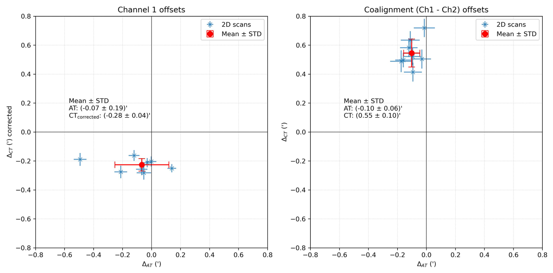
Figure 5 A 2D visualisation of the fitted pointing offsets determined from 2D map data observed during LEGA. The fitted parameters are corrected for the change in target angular size during the ∼1 h observation time. Detailed values can be found in Table B1.

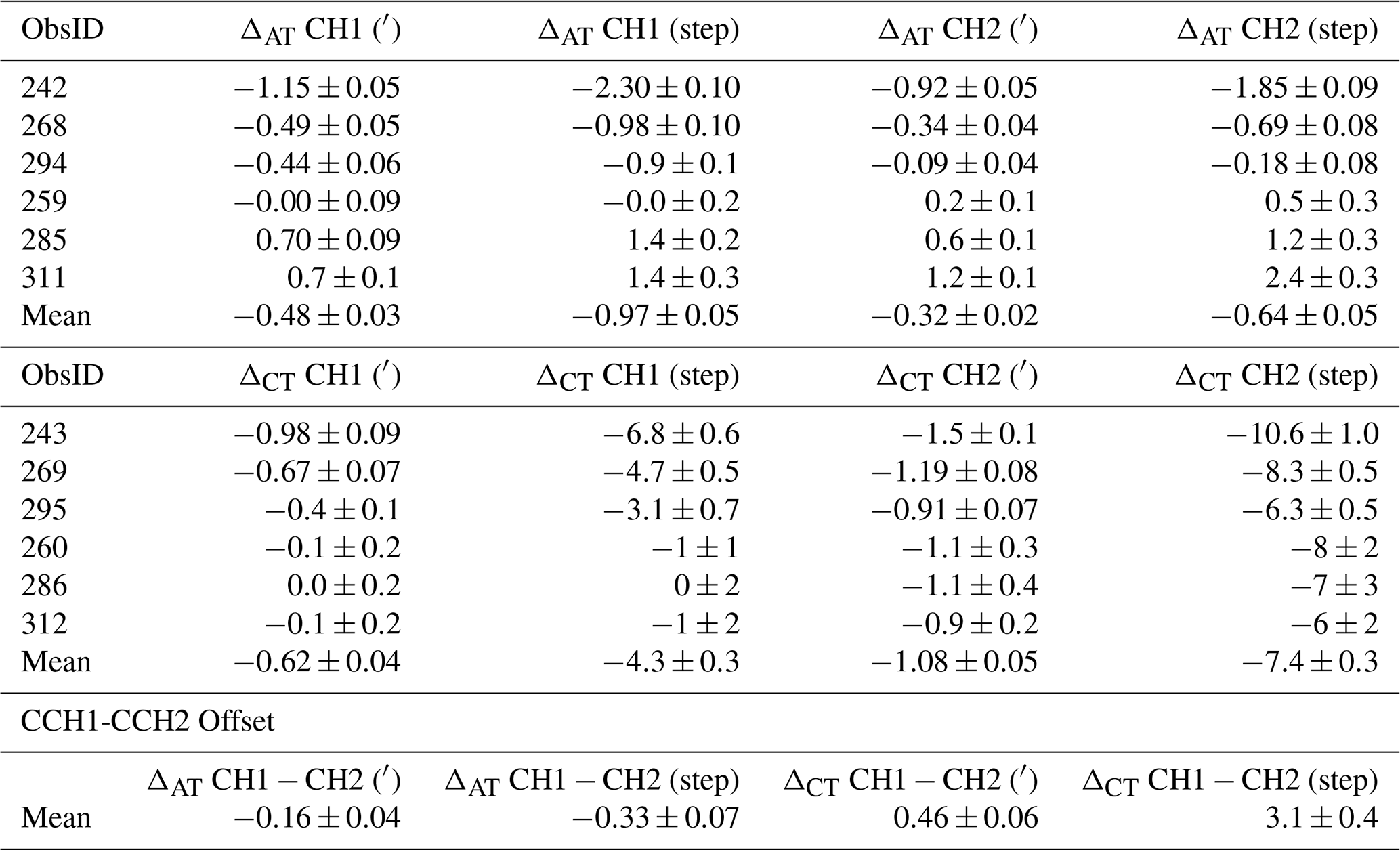
While the 1D scans also offer an opportunity to determine the pointing offsets, our results show that the accuracy of this method is noticeably lower than for the 2D map observations. This is caused mainly by the lower number of points taken during the observation. Nevertheless, we provide the results of our analysis in Table B2. This analysis employed an analogous technique to that of the 2D observations.

Finally, our analysis finds the correction using these maps to be $\mathrm{\Delta }{\text{AT}}_{\mathrm{1}}=(-\mathrm{0.07}\pm \mathrm{0.19}{)}^{\prime }$, $\mathrm{\Delta }{\text{CT}}_{\mathrm{1}}=(-\mathrm{0.28}\pm \mathrm{0.04}{)}^{\prime }$ and $\mathrm{\Delta }{\text{AT}}_{\mathrm{2}}=(\mathrm{0.03}\pm \mathrm{0.18}{)}^{\prime }$, $\mathrm{\Delta }{\text{CT}}_{\mathrm{2}}=(-\mathrm{0.83}\pm \mathrm{0.07}{)}^{\prime }$ and allows to update the AT₀ and CT₀ parameters. These pointing corrections will ensure optimal alignment for future measurements, particularly during Earth Gravity Assist 2 (EGA2) which will occur end of September 2026. The measured receiver coalignement between the 600 GHz (CH1) and the 1200 GHz (CH2) receivers is: Δ (CH1 − CH2) AT $=(-\mathrm{0.10}\pm \mathrm{0.06}{)}^{\prime }$ and Δ (CH1 − CH2) CT $=(+\mathrm{0.55}\pm \mathrm{0.10}{)}^{\prime }$, respectively.

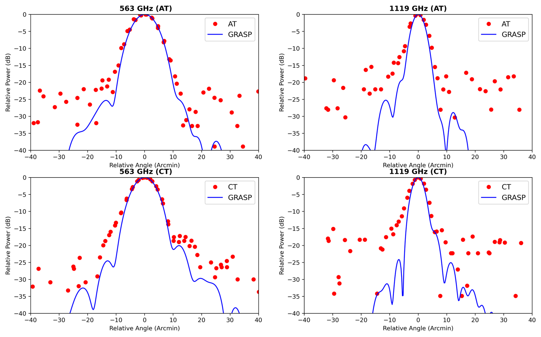
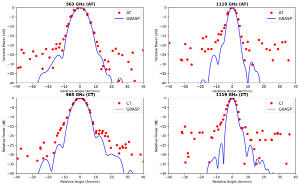
Figure 6 Full antenna beam patterns obtained from 1D scans with a 2 arcmin sampling (ObsIDs 268, 269, 294 and 295). Simulated beam patterns (GRASP) produced by the instrument optical model (Kotiranta et al., 2026) are overplotted for comparison. The panels are organised by scanning direction, with Along Track (AT) on the top row and Cross Track (CT) on the bottom row. The left and right columns show data for channel 1 and channel 2, respectively.

4 Sidelobes and Beam efficiency

Our approach for characterising the beam, described in Sect. 3.1, has also been used to estimate the levels of the side lobes. We have combined all the measurements obtained using the finest sampling (2 arcmin) 1D scans in order to improve the sampling and accuracy (Fig. 6), and compared them with the simulated far-field radiation pattern produced by the instrument optical model. The optical model was created using the GRASP software package¹ by Kotiranta et al. (2018) and recently improved by Kotiranta et al. (2026) taking into account the measured misalignments and surface deviations of the optical components as well as the simulated temperature distortions. We compared the observations with the Grasp optical model calculated at the LO frequency corresponding to that of the measurements. It should be noted that the frequency difference between the LSB and USB bands causes a slight variation in the beam size, on the order of ±1 %. Neverthless, we do not expect any significative change in the sidelobes spatial distributions. Overall, there is good agreement between the measurements and this model. Nevertheless, some parts of the first sidelobe appear to be more intense than expected. Despite limited data (the noise level is about 25 and 18 dB for CH1 and CH2, respectively), we can determine that the first sidelobe in channel 1 contributes at a level of $\sim -\mathrm{16}\mathrm{dB}$ near ±12 arcmin in CT, and for channel 2 we tentatively estimate a value of $\sim -\mathrm{13}\mathrm{dB}$ near ±6 arcmin in both AT and CT. The extended main beam does not appear to be perfectly symmetrical, exhibiting a broadening or “shoulder” at negative offsets, which is particularly pronounced at CT 1119 GHz. In the future, 2D maps (although they require a significant amount of observation time) could allow for a more detailed study of this feature.

We attempted to apply the same methodology to the 1D scans with sampling (4 arcmin and 6 arcmin) and the 2D maps; however, they unfortunately lack either sampling or signal-to-noise ratio to be suitable for such analysis.

4.1 Beam Efficiency

In ground based millimeter radioastronomy, and following the calibration scheme described by Kramer (1997), the main beam efficiency (B_eff) corresponds to the received power that enters the main beam (mb = 3 × FWHM):

$$\begin{array}{}\text{(6)}& B_{\mathrm{eff}}=\underset{\mathrm{mb}}{\int }g\left(\mathit{\theta }\right)\mathit{\theta }\mathrm{d}\mathit{\theta },\end{array}$$

This corresponds roughly to the main beam down to the first null of the simulated diffraction pattern.

Whilst the forward efficiency (F_eff) corresponds to the received power in the forward beam:

$$\begin{array}{}\text{(7)}& F_{\mathrm{eff}}=\underset{\mathrm{2}\mathit{\pi }}{\int }g\left(\mathit{\theta }\right)\mathit{\theta }\mathrm{d}\mathit{\theta },\end{array}$$

To obtain fully calibrated spectra, a relationship must be established between the main beam temperature (T_mb) and the measured antenna temperature (T_a) using the formula:

$$\begin{array}{}\text{(8)}& T_{\mathrm{mb}}=C_{\mathrm{eff}}\times T_{\mathrm{a}}={\displaystyle \frac{F_{\mathrm{eff}}}{B_{\mathrm{eff}}}}\times T_{\mathrm{a}}.\end{array}$$

During the LEGA observations, we did not measure these efficiencies, as the Earth's apparent diameter was too large, i.e. not sufficiently point-like. To estimate the B_eff efficiency, we performed a numerical integration over the simulated beam patterns from Kotiranta et al. (2026) with GRASP – shown in Fig. 6 – within the main beam (3 × FWHM, see Eq. 6) and also computed similarly the F_eff efficiency using Eq. (7). Finally, we can thus determine the GRASP calibration efficiency factor C_eff, which was found to be 1.0245 at 562.95 and 1.0493 at 1119.33 GHz. Therefore, the GRASP calibration correction factor is estimated to be less than few %, and this estimation is also in agreement with the comparison with the Earth model observations in nadir viewing geometry by Jarchow et al. (2026), who found that most of the calibrated brightness temperatures deviate by less than 5 % from the modeled value.

5 Conclusions

The data analysis of the LEGA observations dedicated to the SWI antenna beam allowed us to characterise the antenna pointing and beam pattern in several respects:

1. The beam FWHM is best measured by fitting the 1D scan. Combining NECP and LEGA measurements, the mean weighted FWHM values are (8.18±0.02) arcmin and (4.60±0.03) arcmin at 562.95 and 1119.33 GHz, respectively

2. The pointing offsets are best characterised using the 2D map observations, and our analysis finds the correction using these maps to be $\mathrm{\Delta }{\text{AT}}_{\mathrm{1}}=(-\mathrm{0.07}\pm \mathrm{0.19}{)}^{\prime }$, $\mathrm{\Delta }{\text{CT}}_{\mathrm{1}}=(-\mathrm{0.28}\pm \mathrm{0.04}{)}^{\prime }$ and $\mathrm{\Delta }{\text{AT}}_{\mathrm{2}}=(\mathrm{0.03}\pm \mathrm{0.18}{)}^{\prime }$, $\mathrm{\Delta }{\text{CT}}_{\mathrm{2}}=(-\mathrm{0.83}\pm \mathrm{0.07}{)}^{\prime }$. This ensures optimal alignment for future measurements during the Earth Gravity Assist 2 (EGA2) campaign, after updating the onboard parameters AT₀ and CT₀.

3. The measured receiver coalignement between the 600 GHz (CH1) and the 1200 GHz (CH2) receivers is: Δ (CH1 − CH2) AT $=(-\mathrm{0.10}\pm \mathrm{0.06}{)}^{\prime }$, Δ (CH1 − CH2) CT $=(+\mathrm{0.55}\pm \mathrm{0.10}{)}^{\prime }$.

4. The sidelobes have been measured, with the first sidelobe in channel 1 contributing at a level of $\sim -\mathrm{16}\mathrm{dB}$ near ±12 arcmin in CT, and for channel 2 we tentatively estimate a value of $\sim -\mathrm{13}\mathrm{dB}$ near ±6 arcmin in both AT and CT.

5. An estimation of the GRASP calibration efficiency factor C_eff has been derived by numerical computation using the full beam pattern simulated by Kotiranta et al. (2026), and was found to be 1.0245 at 562.95 GHz and 1.0493 at 1119.33 GHz.

During the EGA2 campaign in September 2026, we plan to perform more SWI observations to improve the accuracy of the beam characterisation (FWHM, pointing offsets, sidelobes, efficiencies) and to monitor the instrument behaviour.

Appendix A: Observation summary tables

Table A1 Observation summary for 1D scans, part 1/2. Values which evolve with time are taken at the beginning of the observation. The keywords are described hereafter. Target: is the name of intended target. Date: is the date of the observation. Start time: is the starting time of the observations. Duration: is the total observation time. Distance: is the Target-center to spacecraft distance. Angular: is the Angular diameter of the target. PSR: is the planet spatial resolution. PSR=Angular/FWHM(CH₁)). Polar angle: is the angle formed between the spacecraft's y axis and the projection of the target's rotational axis onto the spacecraft's xy plane. Phase angle: is the angle between the Sun and the spacecraft measured at the target center. Radial vel: is the radial component of the spacecraft velocity with respect to the sub-SC point. LO1/2: Local oscillator frequency for channel 1 or 2. Molec1/2: Label for intended molecular detection for channel 1 or 2. T_ON: ON source integration time per measurement for CTS or ACS. T_ONCCH: ON source integration time per measurement for CCH. AT/CT OFFSET: Angular deviations of AT and CT of a target with respect to the SC +z axis, as mapped onto the SC x and y plane. SUB SC LAT/LON: Planetocentric latitude/Longitude of the sub-SC point. SUB SUN LAT/LON: Planetocentric latitude/longitude of the subsolar point. MAP DIM: indicating the number of rows and columns of the 2D map. Average step: scan sampling step. Scan direction: 1D scan direction either AT or CT.

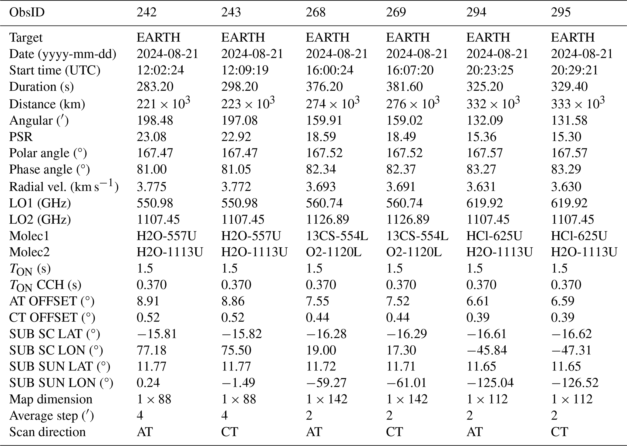
Table A2 Observation summary for 1D scans, part 2/2. Values which evolve with time are taken at the beginning of the observation. The keywords are described in Table A1.

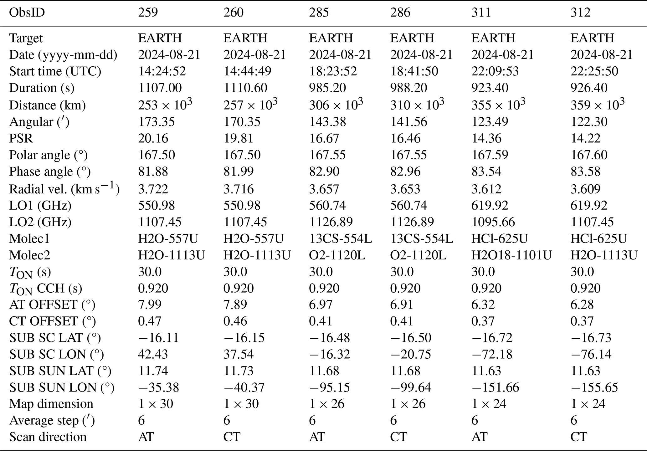
Table A3 Observation summary for 2D maps observed after LEGA. Values which evolve with time are taken at the beginning of the observation. The keywords are described in Table A1.

Appendix B: Pointing offsets

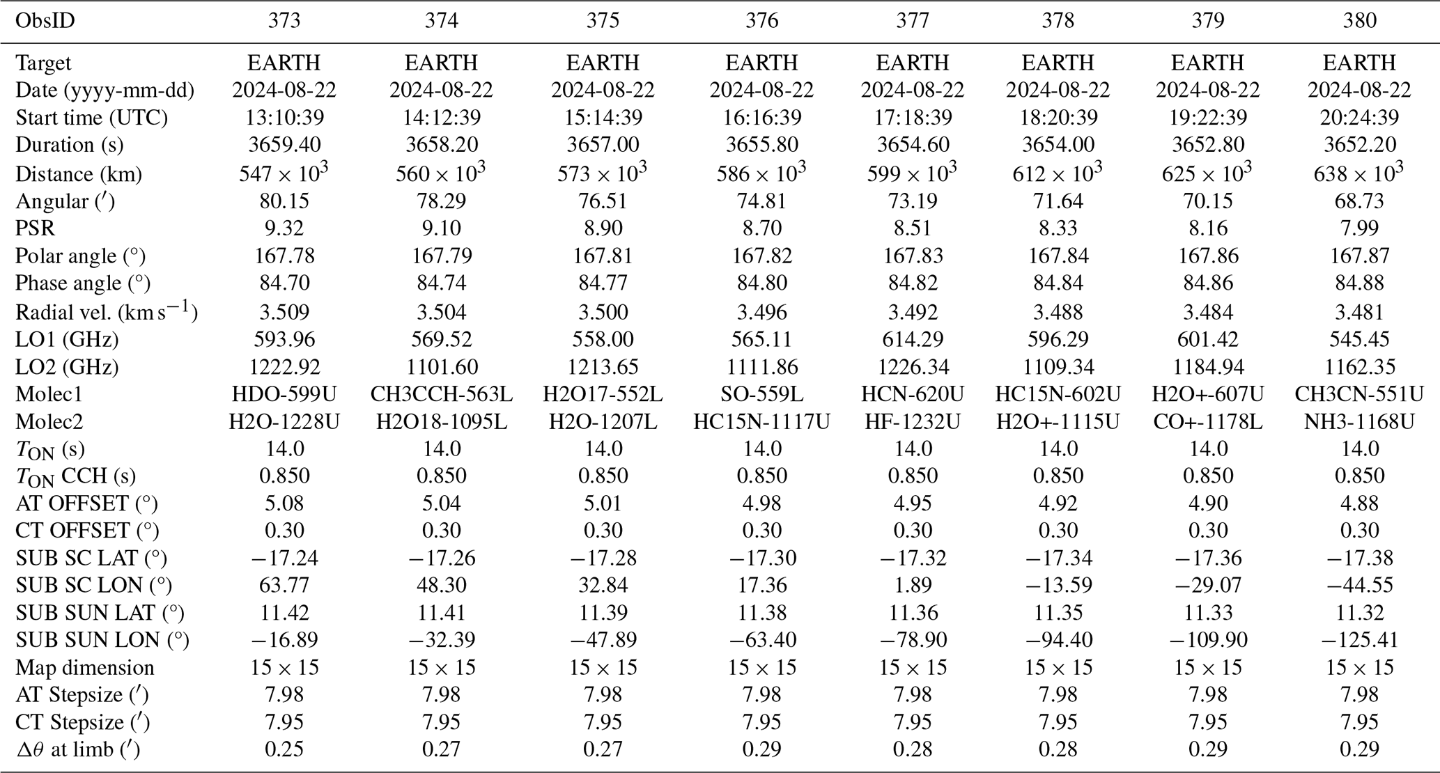
Table B1 Parameters obtained by fitting 2D maps after LEGA without the correction for change in target angular size.

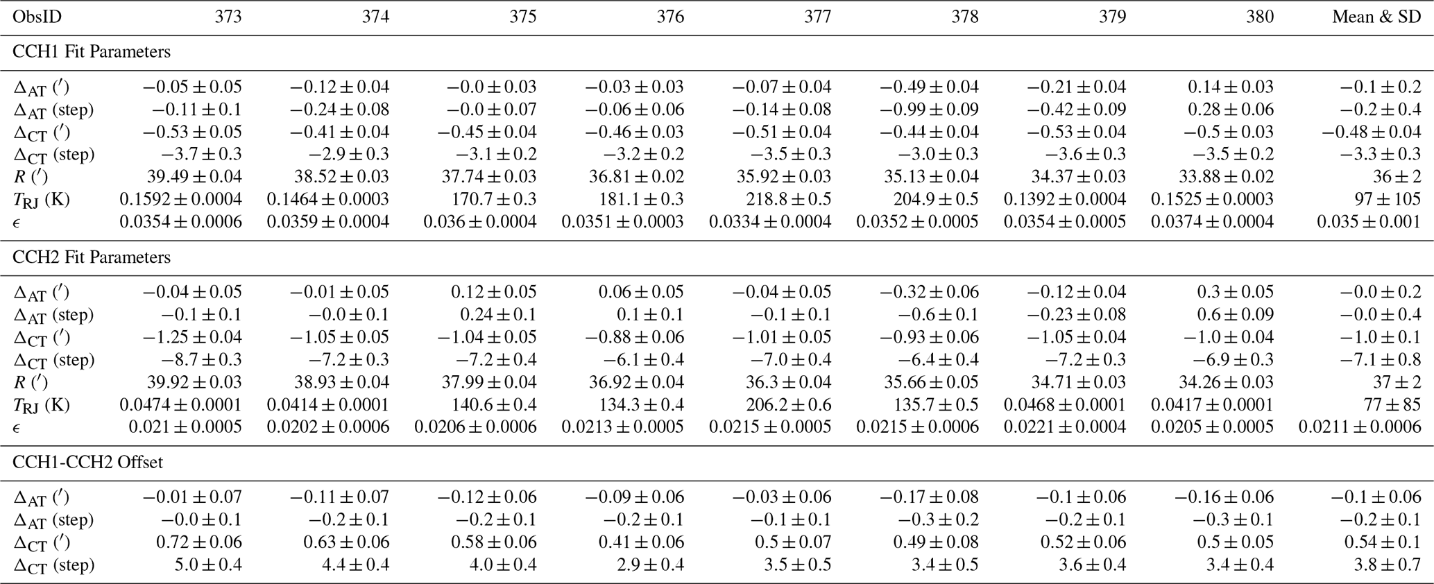
Table B2 Fitted offsets and coalignment of the pointing centre for AT and CT obtained from the data of 1D scans.