Ion composition of the Earth plasmasphere observed by the PEP JEI and RPWI instruments on the JUICE spacecraft

During the first Earth gravity assist maneuver of JUICE on 20 August 2024 the spacecraft passed through the Earth plasmasphere for about 2 h. Before closest approach at a distance of 2.1 R_E the Jovian Electron and Ion spectrometer JEI of the PEP instrument suite was switched on for 40 min in an ion mode test configuration. The high plasma density of about 3000/cm³ (observed by the RPWI plasma wave instrument) led to a negative charging of the spacecraft which allowed a rare observation of the cold and dense plasmaspheric ion populations. Since the ions are only corotating with the Earth at a velocity of about 1 km s⁻¹ at this distance the observed ion speed is dominated by the spacecraft velocity of about 8 km s⁻¹. For this reason ions with different mass appear at different energies in the energy spectrum observed by the JEI sensor. In addition the spacecraft potential leads to specific filtering of ion masses in the observed angular distribution. By calculating the sensor response function for these specific observing conditions it is possible to quantify densities of the different ion species. This response calculation depends critically on the response of the JEI channel electron multipliers to the ion velocity and mass. Since the sensor was operated with a low post-acceleration further laboratory calibrations may be needed for this specific setup. Nevertheless we can already conclude from the observations that ions with mass > 4 amu q⁻¹ contribute at least 25 % to the observed total ion density. A flux peak observed in the energy spectrum at 15 eV can only be explained by the presence of heavy molecular ions with mass ∼ 30 amu q⁻¹. Molecular ions have only been rarely detected in the outer Earth plasmasphere. The observations indicate that the JEI sensor can also be used to achieve ion composition measurements in the exospheres of the Jovian moons.

1 Introduction

On the 20 August 2024 the JUICE spacecraft (Grasset et al., 2013) made its first gravity assist maneuver at Earth with a closest approach altitude of 6850 km corresponding to a L-shell of 2.31 R_E. At this distance from Earth the spacecraft encountered the Earth plasmasphere and several sensors – originally designed for measurements at Jupiter – were able to make new observations of the Earth plasmasphere. Here we report on the measurements of the Jovian Electron and Ion spectrometer (JEI) which is one of the thermal plasma sensors of the Particle Environment Package (PEP, Barabash and PEP-team, 2026) onboard JUICE. The observations are supported by measurements made by the Radio & Plasma Wave Investigation (RPWI, Wahlund et al., 2025).

The Earth plasmasphere is a region of dense cold plasma extending between +1.5 and about 6 Earth radii (R_E) around the center of Earth (Darrouzet et al., 2009). The plasmaspheric ion density is usually > 10³/cm³ within 3 R_E with a plasma temperature < 1 eV (Genestreti et al., 2017). Because the plasmaspheric ion population is rotating close to corotation with Earth, it has very low energy (< 10 eV) in the frame of typical spacecraft observations. This means the ion properties can only be measured in-situ with retarding potential analyzer (RPA) techniques or when the spacecraft charges negatively. The first detailed analysis of the effect of the spacecraft potential on the plasmaspheric spectrum was provided by Whipple et al. (1974) using data obtained by the RPA instrument on the OGO-3 satellite. The most relevant cold ion composition measurements available until today were made by the RPA instrument RIMS onboard Dynamics Explorer 1 (DE 1) between 1981 and 1984 (Roberts et al., 1987). The RIMS instrument could in principle measure ions up to mass 32 amu q⁻¹ (Chappell et al., 1981); the continuously downlinked dataset contains only observations of H⁺, He⁺, ${\mathrm{He}}^{++}$, O⁺ and ${\mathrm{O}}^{++}$ (Roberts et al., 1987). This dataset was reviewed by Goldstein et al. (2018) where it is stressed that specifically the oxygen density of the outer plasmasphere (> 2 R_E) is highly variable and can reach beyond 1000/cm³ such that a specific oxygen torus might form. But on a single specific orbit during a magnetic storm the RIMS instrument was operated in a mode which allowed observation of heavier ions up to mass 46 (Craven et al., 1985). On this orbit a strong flux of ions with 28, 20 and 32 amu q⁻¹ with similar relative abundance was observed stretching from L = 1.1 to 3 R_E. These were interpreted as ${\mathrm{N}}_{\mathrm{2}}^{+}$, NO⁺ and ${\mathrm{O}}_{\mathrm{2}}^{+}$ ions. Interestingly the flux at larger distances was observed to be accelerated along the magnetic field. These observations agreed with earlier observations by the ion mass spectrometer on the ISIS-2 spacecraft during a magnetic storm at 1400 km altitude (Hoffman et al., 1974). The accelerated thermal plasma was even sometimes observed at the Earth magnetopause (Sauvaud et al., 2001). Recently Yue et al. (2023) also reported on observations of plasmaspheric cold ions by the the Van-Allen-Probe HOPE instrument. All observations of molecular ion outflow from the ionosphere up to 2022 were reviewed by Lin and Ilie (2022) and Yamauchi et al. (2024). From these reviews it becomes clear that all more recent observations are for energized outflow (with energies > 100 eV) while the cold plasmaspheric composition has not been observed again after the DE-1 measurements in 1984. A problem with the DE-1 measurements was that the spacecraft potential was not observed by an independent instrument during the observations (Comfort et al., 1985). Ion temperature and potential were obtained by an iterative fit to the data resulting in a plasmaspheric ion temperature of about 3000–5000 K (0.27–0.45 eV) at L = 2 R_E (Comfort, 1996). But the authors emphasize that without knowledge of the potential the ion temperature may be overestimated. The importance of the cold ion population for magnetospheric dynamics was discussed by Delzanno et al. (2021): the cold plasma dominates the solar wind contribution in several magnetospheric regions, it affects the reconnection and instability rates, controls the generation of waves and pulsations. Nevertheless the cold plasma is difficult to observe and observations are rare. A comprehensive review of the instrumental limitations of cold ion observations can be found in Maldonado et al. (2023).

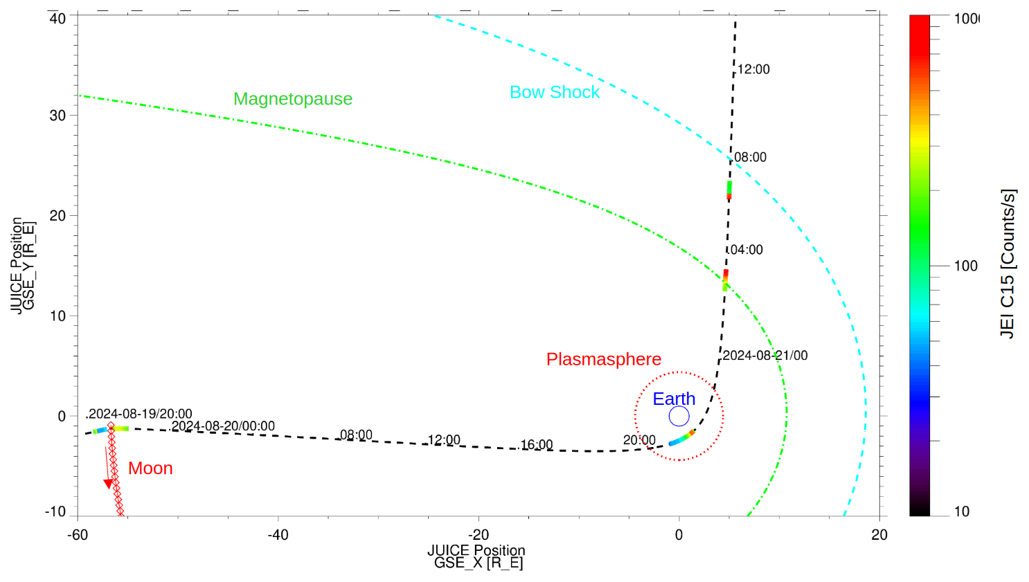
Figure 1 Trajectory of JUICE (black line) during the flyby of the Moon (lower left corner, red crosses) and the Earth on 21 August 2024 in the GSE XY plane. The different lines show nominal position of the plasmapause (red, dotted) (Larsen et al., 2007), the magnetopause (green, dash dot) (Shue et al., 1998) and bow shock (cyan, dashed) (Lu et al., 2019). The colored sections along the JUICE trajectory show the operation times of PEP JEI where the color indicates the count rate observed in channel 15.

The rather high plasmaspheric temperatures (> 0.5 eV) compared to ionospheric temperatures (< 0.1 eV) observed by these early RPA instruments did pose a problem for plasma theory because no sufficient heating mechanism could be identified (Gringauz, 1983). Proton temperatures were again determined from 1996–2001 by the RPA instrument on the MAGION-5 sub-satellite of the INTERBALL 2 mission. Analysis of this data set by Kotova et al. (2008) showed that the temperature of the inner plasmasphere is closely correlated to the temperature of the upper ionosphere. Local temperature is anti-correlated to local density and drops to values below 2000 K (0.18 eV) for densities > 2000/cm³ confirming that the earlier RPA analyses may have overestimated the temperatures. The plasmaspheric temperature observations were discussed again in context of the Van-Allen-Probe mission (Genestreti et al., 2017) where proton temperatures were determined by indirect methods for two orbits confirming the results of Kotova et al. (2008). We note that the Van-Allen-Probe spacecraft charged positive in the plasmasphere which inhibited the direct observation of cold ions (Jahn et al., 2020).

Figure 2 Trajectory of JUICE (blue symbols) during the flyby of the Earth on 21 August 2024 in the GSE XY plane. The red dotted line shows the nominal position of the plasmapause (Larsen et al., 2007). The colored section along the JUICE trajectory shows the operation time of PEP JEI where the color indicates the count rate observed in channel 15. Blue arrows indicate the JUICE velocity vector direction.

2 The observation by the JUICE spacecraft

The ESA spacecraft JUICE was launched on 14 April 2023 on its long mission to planet Jupiter. Between the 19 and 21 August 2024 the spacecraft conducted the first ever Lunar–Earth gravity assists (LEGA) maneuver. The trajectory of the spacecraft during the Lunar–Earth flyby is shown in Fig. 1 projected onto the geocentric solar ecliptic (GSE) XY-plane. Overplotted are the orbit of the Moon (red crosses), the expected position of the Earth plasmapause (red dots), magnetopause (green) and bowshock (cyan). The JEI sensor of the PEP instrument suite (Barabash and PEP-team, 2026) was switched on only during 4 time intervals of length 40 min. These 4 intervals are indicated by the coloring along the JUICE trajectory which shows the count rate observed by channel 15 of the JEI sensor, which shows the highest count rates. The intervals were chosen to obtain electron measurements around the Moon and magnetopause and ion measurements in the plasmasphere and around the bow shock. In this paper we only discuss the observations made during the plasmasphere crossing. An enlarged plot of this crossing is shown in Fig. 2 in the same coordinate plane as Fig. 1. The JEI sensor obtained science data on 20 August 2024 from 21:19 to 21:56 UTC just before closest approach to the Earth at 21:56:14 UTC. At this point the JUICE spacecraft had a distance of 13 211 km or altitude of about 6850 km at geographic latitude 24.0° and L-shell 2.31 R_E.

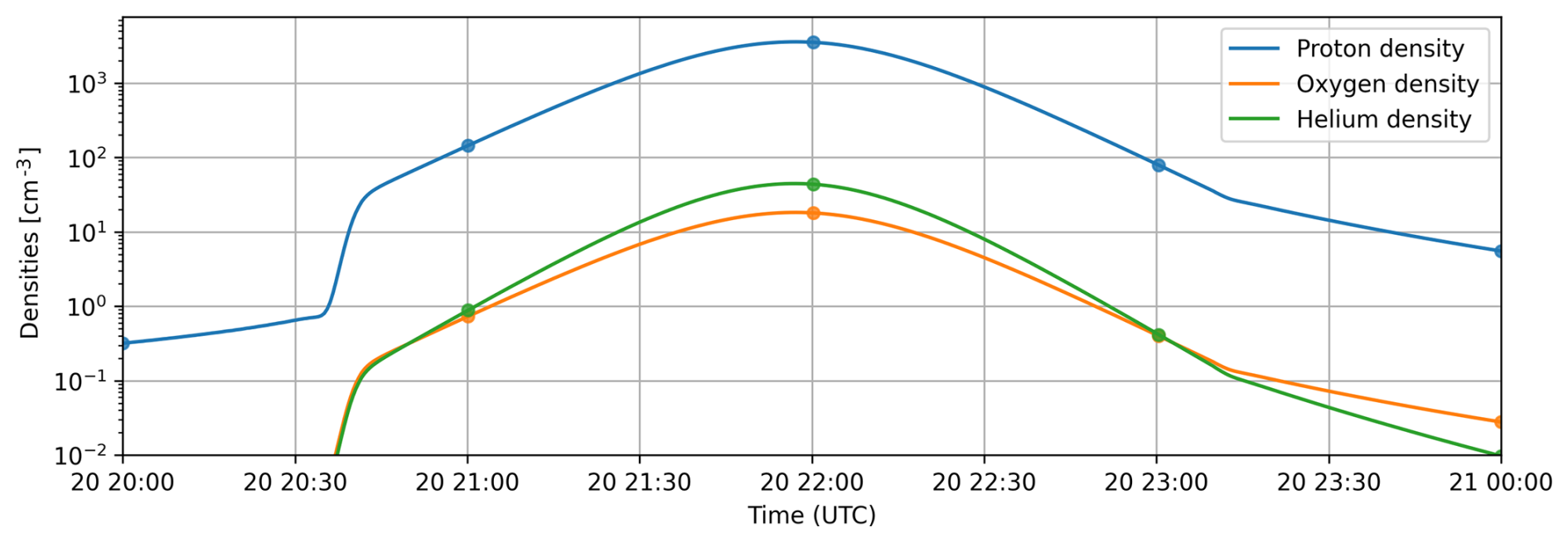
Figure 3 H⁺, He⁺ and O⁺ densities predicted for the trajectory on the 20 August 2024 of JUICE by the Earth global core plasmasphere model (GCPM v2.4, Gallagher et al., 2000).

Figure 3 shows the densities of H⁺, He⁺ and O⁺ predicted for the position of JUICE by the Earth global core plasmasphere model (Gallagher et al., 2000) for a Kp value of 1.7 which was prevalent during the JUICE closest approach (https://kp.gfz.de/en/, last access: 16 October 2026). The model predicts a sharp inbound plasmapause. The authors of the model note that specifically the O⁺ density is highly variable and the model assumes constant initial ratios of 0.1 for He⁺ and 0.01 for O⁺ relative to H⁺. Molecular ions are not contained in the model. We may just consider the total peak ion density value of about 4000/cm³ predicted by the model and note that the SPICED model for the equatorial plasmasphere predicts for L = 2 R_E and MLT = 6 h an average density of 2200/cm³ (James et al. (2021), their Fig. 12).

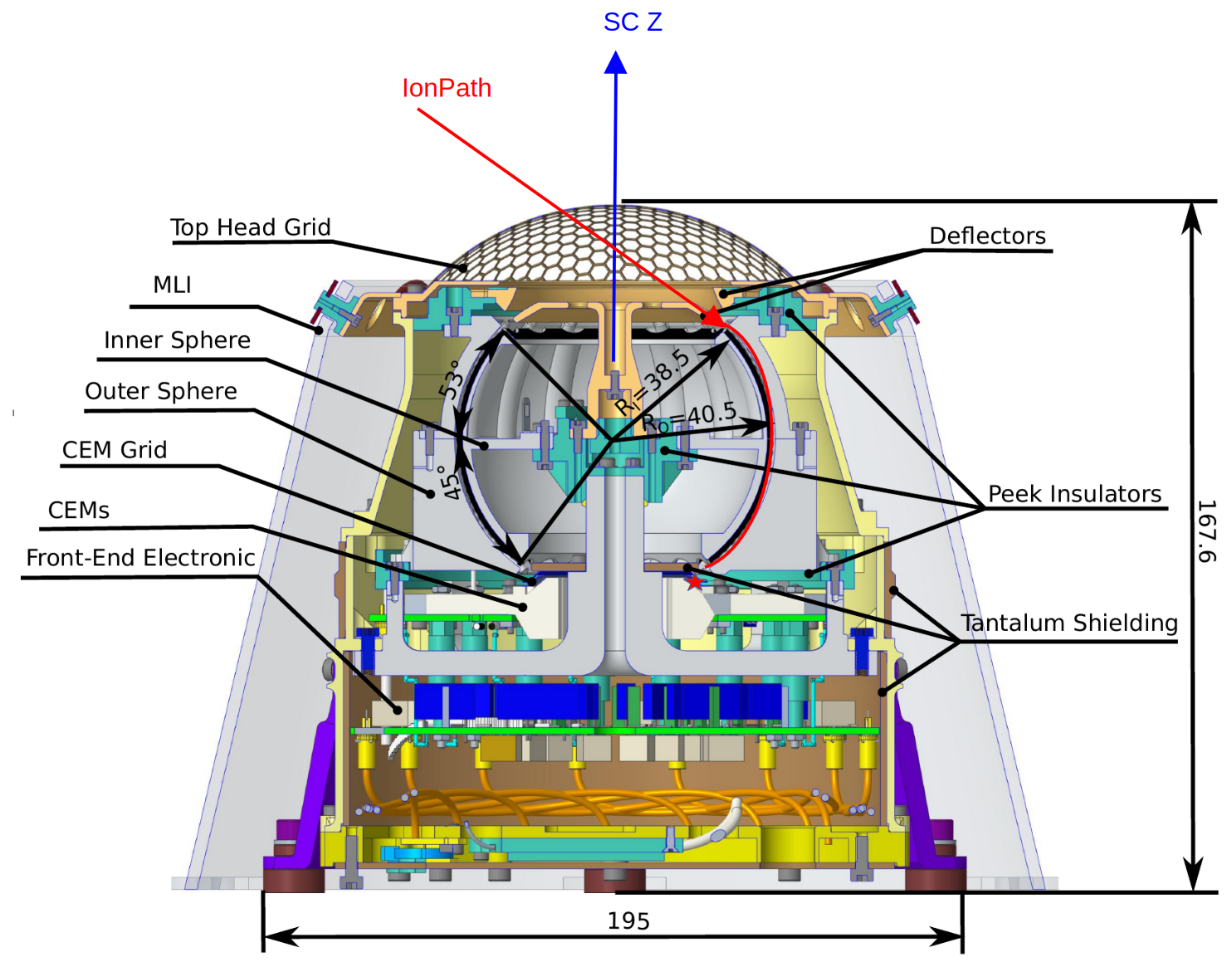
Figure 4 Cross-sectional view of the JEI sensor showing the principal components. The sensor is a spherical electrostatic analyzer with an “open-head” deflection system. Before ions or electrons (red trace) enter the spherical electrostatic analyzer the possible polar entrance angle is set by the deflectors. After the electrostatic analyzer ions are post-accelerated towards the ceramic channel electron multiplier (CEM) entrance, where they create an electric signal (adapted from Bambach, 2026).

2.1 Instrumentation

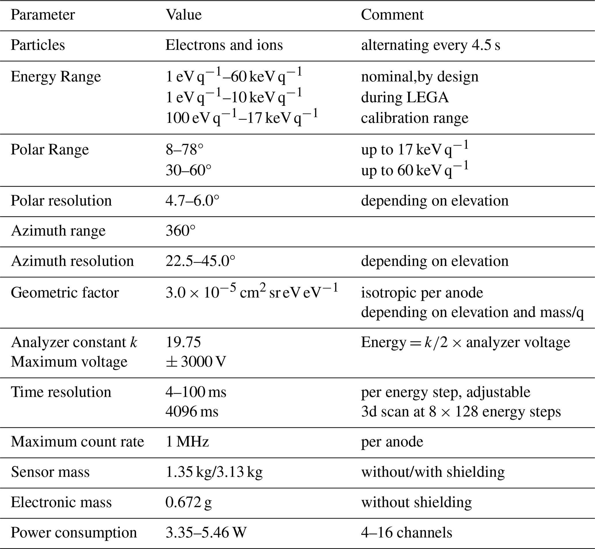
The Jovian Electron and Ion Analyzer (JEI) (Fränz et al., 2017) is one out of six sensors of the Particle Environment Package PEP onboard the Juice spacecraft (Barabash and PEP-team, 2026). It is specifically designed to operate in the harsh Jovian environment. The goals of JEI are to measure the electron and ion distribution functions in the energy range from 1 eV to 60 keV with high sensitivity and time resolution and with a hemispherical field of view. For a full list of sensor properties refer to Table A1. The other sensors of the PEP instrument are the Jovian Neutral Analyzer (JNA), the Neutral and Ion Mass Analyzer (NIM), the Jovian Energetic Neutral and Ion Analyzer (JENI), the Jovian Ion Dynamics and Composition Analyzer (JDC) and the Jovian Energetic Electron Analyzer (JoEE). Only JEI, JDC, JENI and JoEE were operating during the LEGA. Only the JEI and JDC sensors could observe plasmaspheric ions. The observations by JDC are described in an accompanying paper (Stenberg Wieser et al., 2026). The derivation of the spacecraft potential from the Langmuir probe observations of the RPWI instrument on JUICE are described in Wahlund et al. (2025).

Figure 4 shows a cross-sectional view of the JEI sensor with a typical ion path (red). The incoming polar angle with respect to the sensor Z-axis is selected by the deflection system. The ion energy is selected by the spherical analyzer (Inner and Outer Sphere). The polarity of the deflectors and analyzer can be switched to allow measurement of both positive and negative particles including electrons. After post-acceleration charged particles are detected by one of 16 ceramic channel electron multipliers (CEMs), determining the azimuth angle.

The post-acceleration voltage applied between spherical analyzer and CEM entrance we call CEM_head voltage. The detection efficiency is influenced by the CEM_head voltage and the bias-voltage setting across the CEM (CEM_draw voltage). The sensor can operate either continuously in electron or ion mode, or it can alternate between both modes about every 8 s. During the plasmasphere observation JEI was operated in ion mode only with a CEM_head voltage of −250 V and a CEM_draw voltage of +2100 V. At this setting the detection efficiency for protons is about 80 %, the detection efficiency for heavier ions is lower as discussed by Krems et al. (2005). Later during the JUICE mission these voltages will be increased to achieve optimum efficiency.

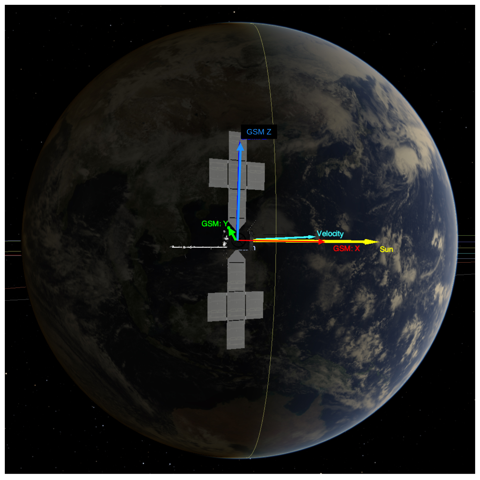
Figure 5 View of Earth from JUICE at 20 August 2024 21:30 UTC with the GSM frame axes. The Earth terminator (yellow) is almost parallel to the GSM Z-axis. The spacecraft velocity vector relative to Earth (cyan) is in the GSM XY-plane. Figure produced by the JUICE Cosmographia software (https://www.cosmos.esa.int/web/spice/cosmographia, last access: 16 October 2026).

JEI has a minimum time resolution of 4 ms per energy step, an intrinsic polar resolution of ∼ 5°, and energy resolution of ∼ 8 % (see Table A1). For a mono-directional beam the energy resolution is around ∼ 5 %. Elevation and energy stepping as well as integration time are set by a look-up-table and change with sensor mode. During the plasmasphere observation integration time was set to 4 ms with a data acquisition time of 3 ms per energy step, polar stepping was set to 8 polar steps covering a polar range from 14 to 75°, and energy stepping was linear in the low energies (0 to 20 eV) with a step width of 0.49 eV and logarithmic for higher energies up to 10 keV with a total of 128 energy steps and a duration of 512 ms for one scan. A complete polar scan using 8 deflector steps takes 4.6 s. The average geometric factor of the angular channel 15 of the sensor has been determined in laboratory calibration as G_E = 3.0 × 10⁻⁵ cm² sr  eV  eV⁻¹ for an isotropic plasma distribution at pre-acceleration voltage of −1000 V with a nitrogen ion beam of 10 keV energy (Bambach, 2026).

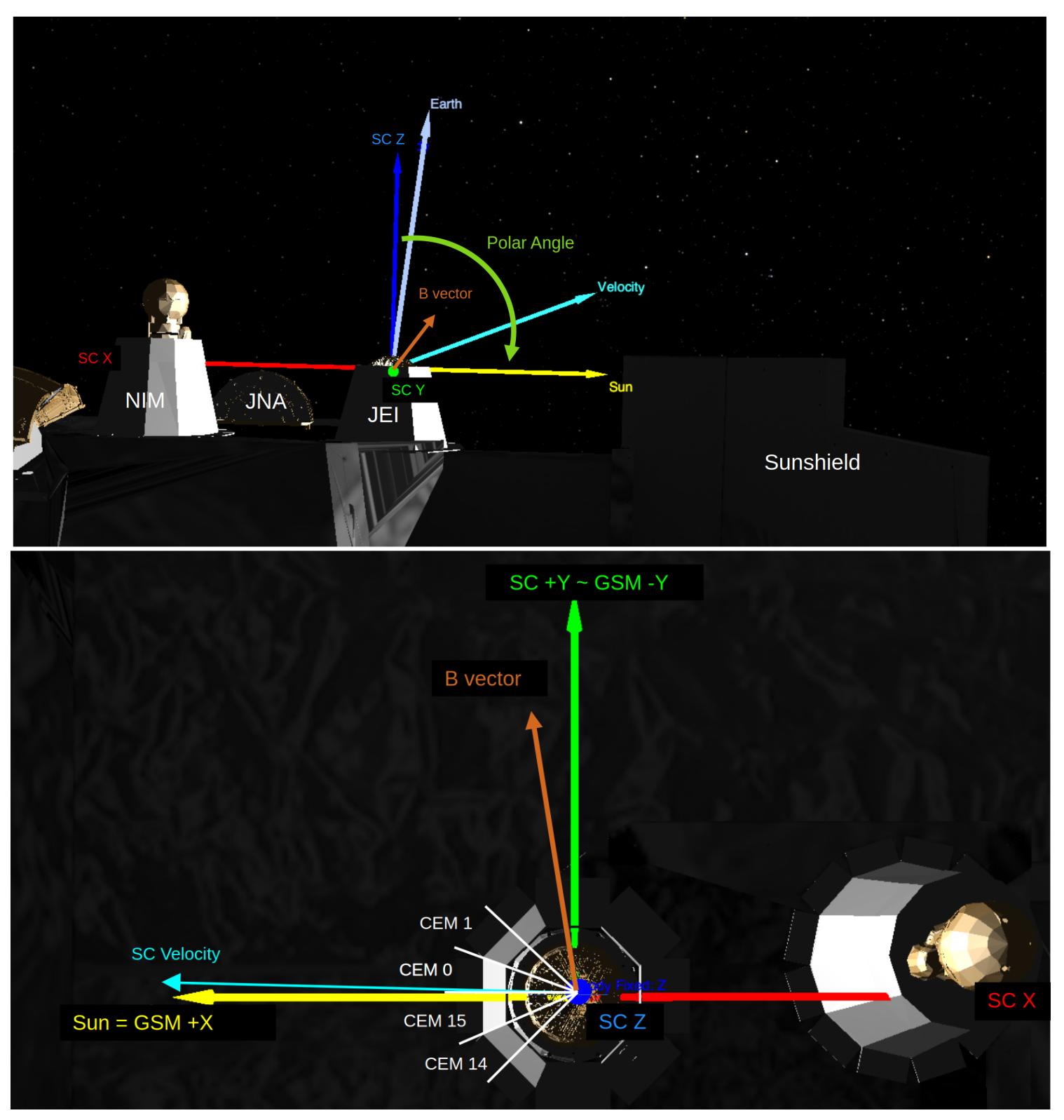
Figure 6 View of PEP sensors on the nadir deck of the JUICE spacecraft. The JUICE JEI coordinate frame orientation (Z = blue, X = red, Y = green, same as spacecraft frame SC) and spacecraft velocity vector relative to Earth (cyan) at 20 August 2024 21:30 UTC are centered at the JEI ion optics entrance. Top: View of the spacecraft frame XZ plane. Bottom: View of the spacecraft frame XY plane, including the field of views of the JEI CEMs. SC +X (red) is opposite to the solar direction (= GSM/GSE +X). SC +Y is approximately parallel to GSM -Y. The model magnetic field vector for 21:30 UTC is shown in brown. Figure produced by the JUICE Cosmographia software.

2.2 Observation geometry

Figure 5 shows the orientation of the JUICE spacecraft relative to Sun (yellow) and Earth together with the orientation of the geocentric solar magnetic (GSM) axes and the spacecraft velocity vector (cyan) at 20 August 2024 21:30 UTC. The yellow line indicates the Earth terminator. This principal orientation of the spacecraft was maintained throughout the observation interval. The PEP JEI sensor is mounted on the spacecraft panel which looks towards Earth during this time. This panel is illustrated in Fig. 6 which shows the location of the NIM, JNA and JEI sensors together with the orientation of the body fixed spacecraft coordinate system axes, the direction of Earth and Sun and the spacecraft velocity vector relative to Earth. The body fixed spacecraft Z-axis coincides with the JEI sensor symmetry axis. The JEI polar field of view extends from 8 to 78° from this axis. In Fig. 6 (right) we also show the field of view of JEI azimuth sectors 1, 0, 15 and 14.

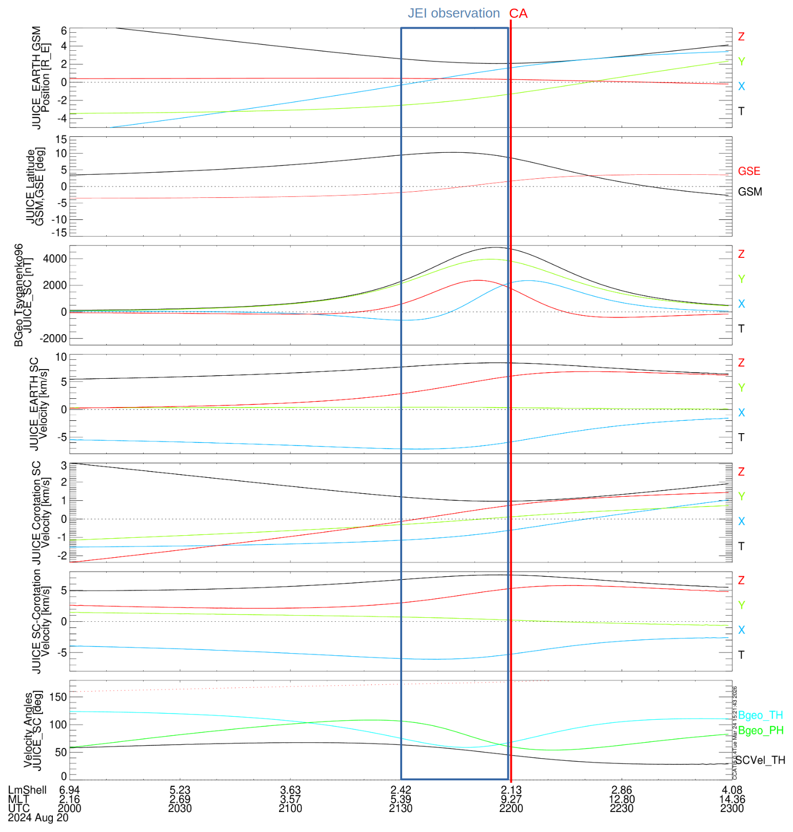
Figure 7 JUICE orbital parameters in Earth centered coordinates for 20:00–23:00 UTC on 20 August 2024 from top to bottom: Position vector components in GSM coordinates, GSM (black) and GSE (red) latitude, Tsyganenko96 geomagnetic field B_geo at JUICE position in spacecraft coordinates, JUICE velocity vector relative to Earth in spacecraft coordinates, plasma corotation vector at full corotation in spacecraft coordinates, difference vector D between JUICE velocity and corotation, θ angle of D (black) and B_geo (cyan) and ϕ angle of B_geo (green). The Tsyganenko field and L_m-shell values are calculated using the IRBEM model of the disturbed geomagnetic field for the solar wind conditions prevalent during the JUICE passage (https://prbem.github.io/IRBEM/index.html, last access: 16 October 2026).

Figure 7 shows position and velocity parameters of the JUICE spacecraft relative to Earth for the period of the plasmasphere crossing, from top to bottom: spacecraft position in GSM coordinates in Earth radii (R_E), spacecraft GSM and GSE latitude, magnetic field B_geo (nT) in spacecraft coordinates predicted by the Tsyganenko96 model (Tsyganenko and Stern, 1996), spacecraft velocity vector (km s⁻¹), and the plasma corotation velocity vector (km s⁻¹), the difference vector D between both in JUICE spacecraft coordinates, and the angles of D and B_geo in spacecraft coordinates. We here assume that the corotation is symmetric around the GSM Z-axis. Models of the corotation predict ∼ 92 % corotation at L = 2.0 (Lejosne et al., 2017). Vector components are indicated by X(blue), Y(green), Z(red) and total T(black). The red vertical line indicates the closest approach (CA) and the blue frame the period of the JEI observation discussed in the following. Calibrated onboard magnetic field data are not available at the time of writing. We observe that the predicted magnetic field vector and the spacecraft velocity vector are both at a polar angle of 50° as seen from the JEI sensor.

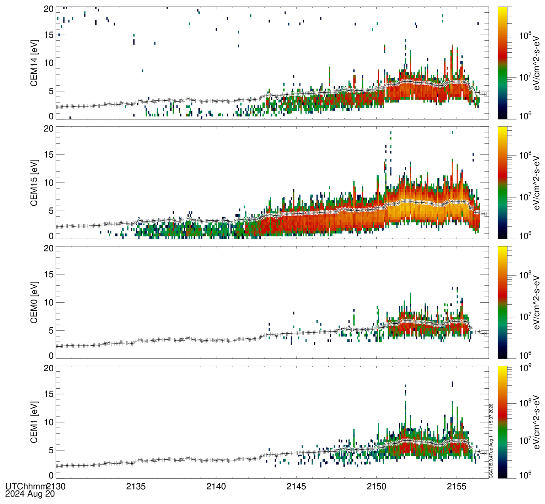
Figure 8 Ion energy spectra observed by PEP JEI in 4 azimuthal viewing directions during the passage of the Earth plasmasphere. The median electronic background noise has been subtracted from the spectra. Black crosses show the negative spacecraft potential observed by JUICE RPWI where the left axis gives the negative voltage. Data are averaged over 8 elevation scans (4.6 s).

2.3 Ion energy spectra and potential

Figure 8 shows the energy spectra obtained by the 4 azimuthal sectors (CEM channels) viewing around the direction azimuth of the spacecraft velocity during the time interval 21:30–21:56 UTC on 20 August 2024. We here show only the spectral energy range 0–20  eV. The higher energy range is dominated by background noise. The white line plotted over the spectra shows the negative value of the spacecraft potential measured by the JUICE RPWI instrument. We observe that all 4 channels observe an intense low energy ion spectrum with a mean energy proportional to the negative spacecraft potential observed by RPWI. The most negative potential measured by RPWI is −6.5 V. The same effect was observed on the opposite side of the spacecraft by the Jovian Plasma Dynamics and Composition analyzer (JDC) of the PEP suite. These observations are discussed in an accompanying paper (Stenberg Wieser et al., 2026). It is interesting to note that the RPA instrument on the OGO-3 spacecraft in 1966 measured at the same L-shell location 1.5–2.5 R_E a very similar potential between −5.0 and −6.0 V at an estimated ion density of about 6000/cm³ (Whipple et al., 1974). This shows that the values observed for JUICE are not uncommon – though the potential value depends on the material properties of spacecraft surfaces. Zeroual et al. (2026) modelled the charging of the JUICE for plasmaspheric conditions at the specific time 21:56 UTC using the SPIS software (https://www.spis.org/software/spis/, last access: 16 October 2026). They derive an average surface potential of −2.0 V, but −4.0 V for the shadowed vault in front of the JEI sensor. Thus the calculated potential is less negative than the observed potential. The difference may be caused by assumptions on the ion and electron temperatures used in the model.

Channel 15 observes the highest flux, though the spacecraft velocity vector is at the edge of the field-of-view of channel 0 (see Fig. 6). As discussed later the reason lies mainly in the differences of the detection efficiency of the CEMs at the low CEM_draw voltage setting. Another effect is that for a small Debye length the shape of the spacecraft potential follows the spacecraft structure (Zeroual et al., 2026). As discussed further in the next section this leads to a significant ion deflection. The rather strong signal in the neighboring channels 1 and 14 indicates that the spacecraft potential has a focusing effect, although we can not exclude some electronic and geometric cross talk between the channels as discussed in Bambach (2026). In the following we only discuss the spectra obtained by channel 15 as this has the best counting statistics. While an acceleration by the spacecraft potential should lead to the cold thermal spectrum observed for most energy scans the sporadic extension of the spectra up to 20 eV caught our attention because they may suggest a non-thermal effect or multi-component plasma.

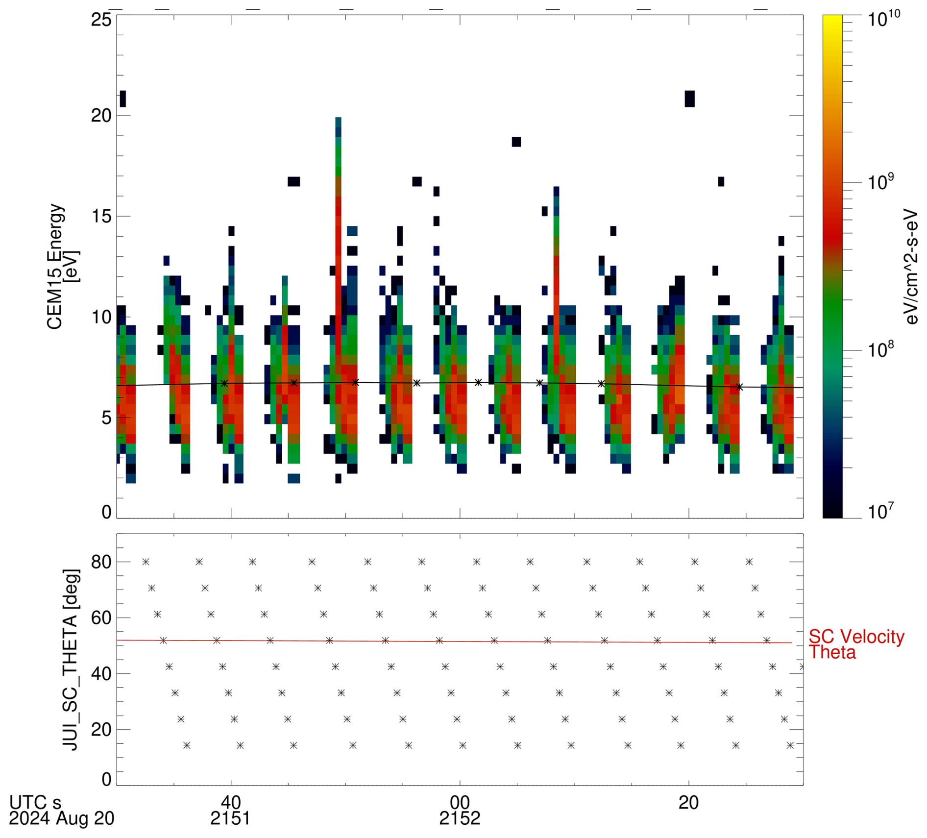
Figure 9 Top: Ion energy spectra observed over 1 min (21:51:30–21:52:30 UTC on 20 August 2024) at 512 ms resolution by PEP JEI CEM15 during the passage of the Earth plasmasphere. The negative of the spacecraft potential value is overplotted in black. Bottom: The median polar angle of each spectra (black stars) with respect to the Spacecraft Z-axis and the polar angle of the JUICE spacecraft velocity (red line) relative to the Earth.

The top panel of Fig. 9 is a zoom into the energy spectra of channel 15 for the one minute time interval between 21:51:30–21:52:20 UTC on 20 August 2024. Overplotted in black is the negative of the spacecraft potential of about −6.5 V measured by RPWI. We observe that the energy spectra show a pattern repeated for each sequence of 8 elevation scans of the sensor. Figure 9 (bottom) shows the mean polar angle of the JEI field-of-view for each spectrum. Overplotted in red is the polar angle of the spacecraft velocity vector relative to Earth. We can see that ions are only observed at polar angles from 14° to about 60°. The mean energy of the spectrum is increasing with polar angle. High energy spikes are only observed twice during this interval at 21:51:49 and 21:51:08 UTC at polar angles of about 35°.

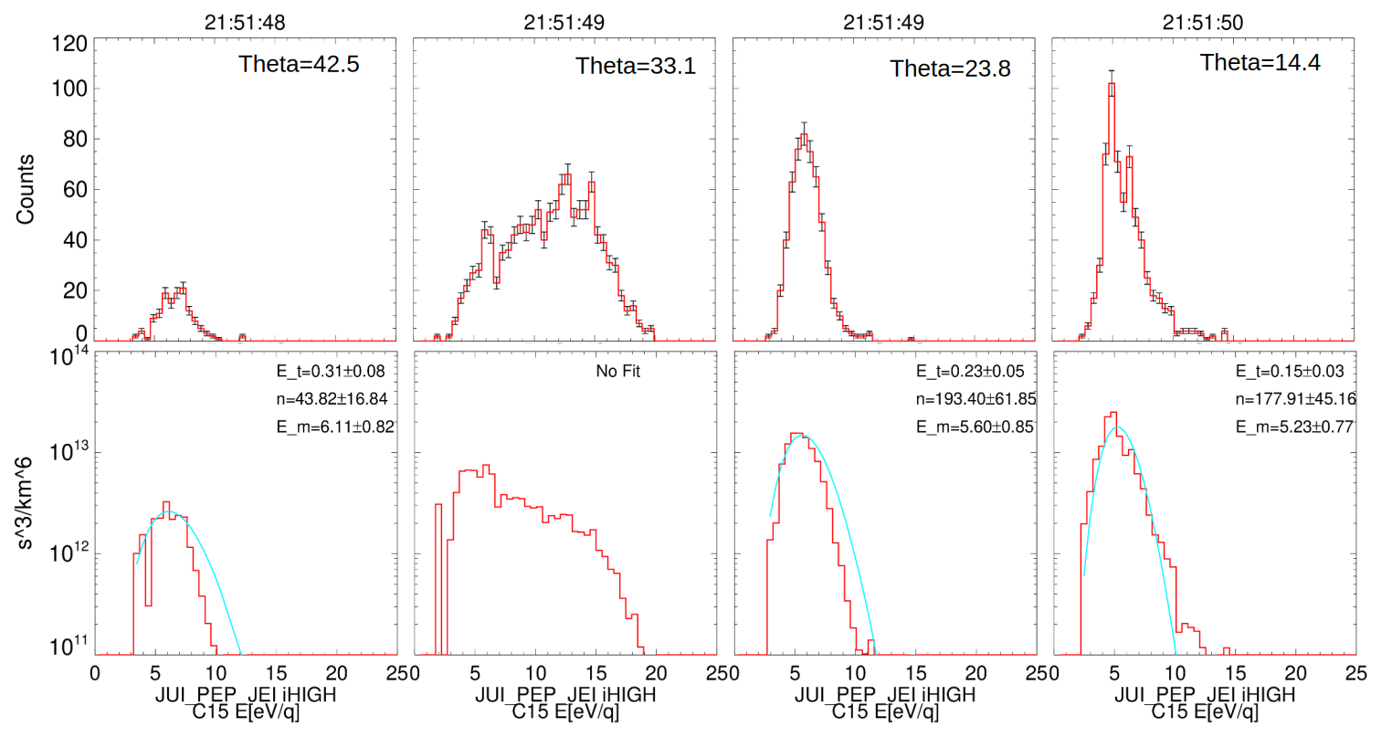
Figure 10 Four individual ion spectra observed in sequence around 21:51:49 UTC on 20 August 2024 by PEP JEI CEM15 without correction for the spacecraft potential. Top: Counts in linear scaling. Bottom: Conversion to phase space density assuming proton mass in logarithmic scaling. Some of the spectra allow a Maxwellian fit to the core distribution shown in blue with the derived parameters temperature (E_t, eV), density (n, $/{\mathrm{cm}}^{\mathrm{3}}$) and mean energy (E_m, eV) in the spacecraft frame of reference.

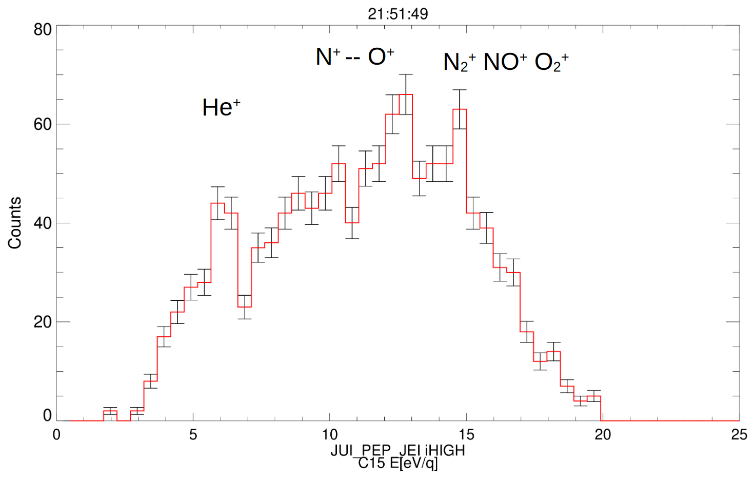
Figure 11 Count spectrum observed at 21:51:49 UTC by PEP JEI CEM15 at a polar deflection angle of 33.1° and attribution of flux peaks to species. The association of the spectral peaks with different ion species is explained in context of Fig. 14 below.

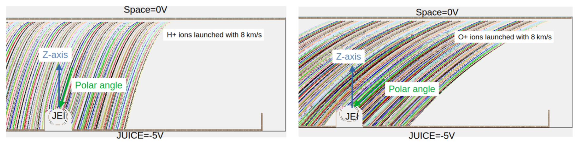
Figure 12 Simion^® simulation of the deflection of H⁺ (left) and O⁺ (right) ions in a linear spacecraft potential. Ions are launched with spacecraft velocity at 1 m distance in a linear potential with scale height 50 cm arriving at the instrument with different polar angles θ.

To further illustrate the effect we show in Fig. 10 four individual spectra obtained in sequence around 21:51:49 UTC at different mean polar angles. The top row of the figure shows the counts obtained in each 3 ms energy bin and the value of the mean polar angle (θ). The energy axes show the energy in the JEI reference frame without correction for the spacecraft potential. We note that the statistical error of these spectra can be obtained by the square root of the counts. The bottom row shows the same spectra converted to phase space density assuming an ion mass of 1 amu and a base geometric factor as provided in Table A1 without considering CEM efficiencies. Spectra which show an approximate Maxwellian shape have been fitted with a Maxwellian with the three free parameters mean energy, temperature and density (see Appendix B). The resulting values and their fit standard deviation are printed in addition to the fitted curve (cyan). The plots are in log scale and the fit parameters are derived from 6 data points with the highest phase space density. We can see that the spectra obtained at polar angles θ = 14.4° and θ = 23.8° can be best approximated by a Maxwellian resulting in ion densities of around 180/cm³, temperatures of around 0.2 eV and mean observed energies around 5.3 eV (including spacecraft potential). As we discuss later the rather low density value as compared to the RPWI value is caused by not considering the potential geometry and CEM efficiency in this simple approach. Further below we try to include these effects and derive much higher density values. When looking closer at the count spectrum obtained at θ = 14.4° one can discern 2 peaks in the spectrum which may indicate a bimodal distribution. The most interesting spectrum is the one obtained at θ = 33.1°. It shows different spectral peaks at higher energies with a statistical significance > 2σ. For this reason we show an enlarged view of this spectrum in Fig. 11 where we associate the different peaks with different ion species as explained in the next section.

To estimate the statistical occurrence of these spectral peaks we counted the number of 4.6 s polar scans with peak energies above 10 eV q⁻¹ for the time period 21:47:00–21:56 UTC when the potential measured by RPWI was more negative than −5.0 V: this was the case for 28 out of 108 polar scans. In all cases the peaking spectrum was observed for polar angles smaller than 30°. In all 108 polar scans the mean energy of the spectrum increased with decreasing polar angle.

Before discussing this observation we need to consider the total plasma density and shape of the spacecraft potential. The JUICE RPWI instrument reports an ion density of 3000/cm³ determined by the Langmuir probe measurement for the time 21:55:17 UTC (Jan-Erik Wahlund, personal communication, 2026). This agrees approximately with the value of 4000/cm³ predicted by the global plasmasphere model (Fig. 3) when taking into account the large temporal variation of the plasmasphere. The electron temperature determined by the RPWI analysis is 0.35–0.5  eV. In this case the plasma Debye length around the spacecraft, which determines the extension of the spacecraft potential, is only about 8.0 cm. This means that the equipotential surfaces follow the shape of the spacecraft structures and must be considered locally as planar and not spherical (see Appendix D). In an accompanying paper Zeroual et al. (2026) discuss the surface charging of the JUICE spacecraft during the Earth gravity assist.

3 Interpretation and model

To illustrate the general effect of a potential with small Debye length on a plasma flow with different ion masses we show in Fig. 12 a Simion^® (https://simion.com/, last access: 16 October 2026) simulation of ion trajectories in a linear and planar potential of V_p = −5 V at spacecraft surface and instrument and 0 V at 50 cm distance. Ions are launched parallel to the spacecraft surface at 50 cm distance with mass per charge of 1 amu q⁻¹ (left) and 16 amu q⁻¹ (right) and a velocity of v_x = 8 km s⁻¹. One can see that the lighter ions reach the JEI sensor at a higher polar angle than the heavy ions. We note that Fig. 12 is for illustration of the principle only. The Simion software can not simulate a potential with exponential fall off caused by Debye shielding. The important assumptions are that the electric field is mainly vertical and ions are launched from a field-free point. In this case the ion acceleration is mainly in vertical direction such that the distance from which ions are launched has no influence on the arrival angle. A more realistic simulation could be done using the SPIS model, cited above.

Table 1 Expected mean polar angle θ relative to SC Z-axis for different initial velocities and SC potentials V_p.

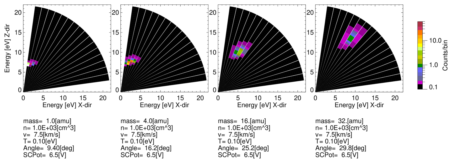
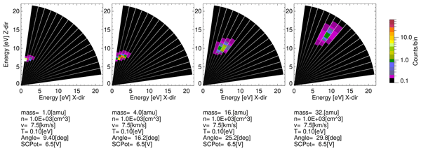
Figure 13 Instrument response calculation including CEM efficiency (Krems et al., 2005) for different ion species arriving under the polar angles listed in the first line of Table 1 with acceleration of a −6.5 V spacecraft potential. Ions shown from left to right are H⁺, He⁺, O⁺ and ${\mathrm{O}}_{\mathrm{2}}^{+}$. We assume for this simulation an initial density of 1000.0/cm³ (in spacecraft frame) per species and an initial velocity of 7.5 km s⁻¹. Shown are the expected counts in each measurement interval of 3 ms per energy bin.

To treat the effect analytically we assume that the potential is planar with respect to the spacecraft nadir deck. In this case the acceleration of ions by the potential is only in -Z direction. The energy gain is given by E_p=qV_p, where V_p is the spacecraft potential and q the ion charge. Since the acceleration is only in -Z direction, we can calculate the observed vertical velocity by $v_z=\sqrt{\mathrm{2}{E}_{\mathrm{p}}/m-\text{sign}\left(v_{z\mathrm{0}}\right)v_{z\mathrm{0}}^{\mathrm{2}}}$, where v_z0 is the initial undisturbed vertical velocity. The sign of the vertical velocity is introduced to cover both ions moving initially towards the spacecraft deck and away from the spacecraft deck. Under the assumption of a planar potential we can then calculate the polar angle θ_p relative to the vertical axis by

$$\begin{array}{}\text{(1)}& \tan {\mathit{\theta }}_{\mathrm{p}}=v_x/v_z={\displaystyle \frac{v_x}{\sqrt{\mathrm{2}q{V}_{\mathrm{p}}/m-\text{sign}\left(v_{z\mathrm{0}}\right)v_{z\mathrm{0}}^{\mathrm{2}}}}},\end{array}$$

where (v_x,v_z0) are the initial velocity components parallel and perpendicular to the spacecraft surface, and $m/q$ is the ion mass per charge. The expected total observed energy per charge is $E/q=\frac{m|v{|}^{\mathrm{2}}}{\mathrm{2}q}+V_{\mathrm{p}}$. In Table 1 we calculate the expected mean inclination angles for different ion species for the conditions valid at around 21:50 UTC where the spectra shown in Figs. 10 and 11 were observed. From Fig. 7 we can read the approximate initial velocities either assuming that the plasma is at rest relative to Earth in the GSE frame or rotating with corotation speed. We here compare expected angles for a spacecraft potential of −5.0 and of −6.5 V as reported by RPWI (Fig. 8). The polar angle of the inflow, when undisturbed by the potential, is about 45°. By Eq. (1) and illustrated in Fig. 12 the expected polar angle becomes smaller with increasing potential. The maximum ion mass we consider is 32 amu q⁻¹ (${\mathrm{O}}_{\mathrm{2}}^{+}$). Earlier observations of heavy molecules in the plasmasphere (Craven et al., 1985) suggest that molecules with mass 28 and 30 amu q⁻¹ (${\mathrm{N}}_{\mathrm{2}}^{+}$ and NO⁺) may be more abundant than ${\mathrm{O}}_{\mathrm{2}}^{+}$. The energy resolution of the JEI sensor does not allow to separate these masses such that ${\mathrm{O}}_{\mathrm{2}}^{+}$ is considered only as representative for the heavy molecular component. Similar spatial effects of the spacecraft potential on the ion distribution were discussed in context of the Rosetta mission (Nyffenegger et al., 2001; Bergman et al., 2020).

We can see from Fig. 9 that ions are observed only for polar angles smaller than 45° in agreement with the expectation that the spacecraft potential decreases the inclination angle. We can also see that spectra observed at inclination angles < 25° show only a single or double Maxwellian distributions as the example shown in Fig. 10 (right panels). Table 1 shows that spectra observed at lower angles should be dominated by light ions – mainly H⁺, He⁺ and ${\mathrm{He}}^{++}$. The high energy tail seen at θ = 14.4° may be contributed by the helium ions. Only at inclination angles > 25° we can see spectra with higher mean energy per charge and separate peaks in the spectrum as shown in Fig. 11. We interprete these as being dominated by heavier ions. Since the peak with maximum energy per charge is observed at 15.0 eV we may conclude from the values shown in the table that:

• 1.

  the energy of the peak count rate observed by the JEI sensor suggests a spacecraft potential of around −5.0 about 1.5 V less negative than the value reported by RPWI, though this can be an effect of difference in the ground reference voltage,

• 2.

  the heavy molecular component is predicted to have a mean energy per charge of 15.6 eV and a predicted mean polar angle of 29.8°,

• 3.

  the smaller flux peaks observed at 5–7 eV q⁻¹ are caused by the thermal spread of the light ion distribution,

• 4.

  the distribution observed between 8 and 13 eV q⁻¹ can be associated with heavier ions. We can for example not exclude contributions by nitrogen ions.

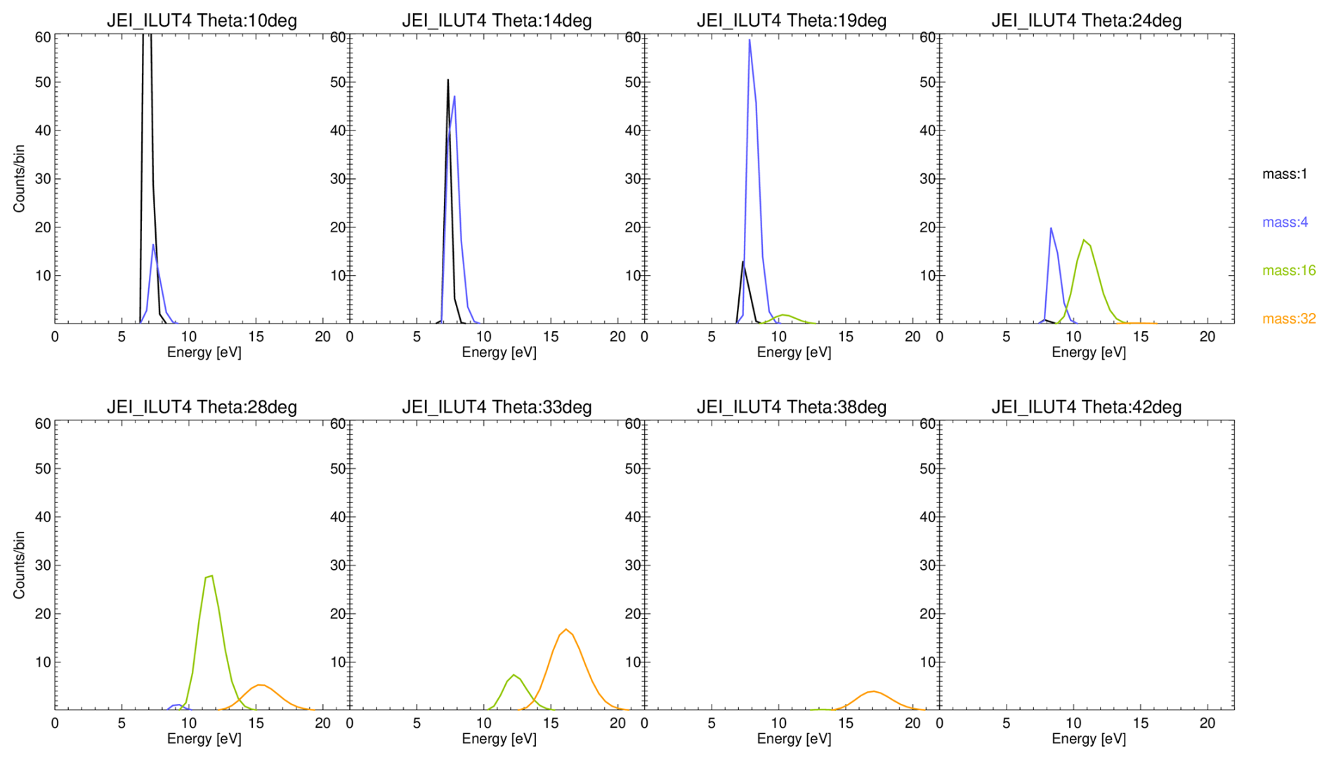
Figure 14 Same simulation setup as for Fig. 13 showing the simulated contribution of different ion species (H⁺ (black line), He⁺ (blue line), O⁺ (green line) and O2+ (orange line)) of same density to the observed count spectra for the upper 8 virtual polar angles (listed on top).

To better quantify the contribution to the spectra shown in Figs. 10 and 11 we made a sensor response calculation for the specific ion species and geometries listed in Table 1. We assume for all ions a common initial velocity of 7.5 km s⁻¹, an acceleration by a −6.5 V potential, a temperature of 0.1 eV and a density of n₀ = 1000/cm³ for each species. We take the same density for each species to later allow a scaling to the observed count rate. We derive the expected phase space distribution for each species as a function of angular distance from the beam center as explained in Appendix C. From the phase space distribution we derive the particle flux using the base geometric factor given in Table A1. But here we also take the polar angle (θ) dependence of the efficiency into account which reduces the geometric factor at smaller polar angles. We also include the dependence of the CEM efficiency on ion mass and pre-acceleration voltage (CEM_head) using the general formula for MCPs from Krems et al. (2005).

Figure 13 shows the expected counts in each energy bin for the inclination angles listed in the first line of Table 1. The integration time per energy bin is 3 ms. The plots divide the polar field-of-view of JEI (10–75°) into 16 sectors of 4.4° width. The JEI sensor was operated during this observation pass with a division of the polar field-of-view into only 8 sectors, but the polar full width half maximum (FWHM) of the sensor for a cold beam is only about 5° such that only every second sector shown in Fig. 13 was observed by JEI. The mean angles of the JEI polar sectors are given in Figs. 10 and 11.

In Fig. 14 we overlayed the predicted contributions of the different ion species to the spectrum observed under the top 8 polar simulation sectors – only 4 of these sectors have been observed by the JEI sensor. These distributions can now be compared with the 4 observed spectra shown in Figs. 10 and 11. Note, that the simulation uses the same density of 1000.0/cm³ for each species. We can see that the spectrum observed at 14.4° can have contributions of H⁺ and He⁺ where the density of 177 ± 45/cm³ obtained by fitting shown in Fig. 10 can not be directly compared because is does not contain the dependence of the efficiency on elevation angle and pre-acceleration voltage of the sensor. To obtain a more realistic density value for H⁺ (assuming that He⁺ is minor) we may multiply the assumed density n₀ by the ratio of the peak counts in Figs. 10 and 14 for the respective θ angles. We then get:

$$\begin{array}{}\text{(2)}& \begin{array}{rl}\mathit{\theta }=\mathrm{14}\mathit{°}:n_{{\mathrm{H}}^{+}}& =n_{\mathrm{0}}\times (\mathrm{100.0}\pm \mathrm{10})/\mathrm{50.0}\\ & =\mathrm{2000}\pm \mathrm{200}/{\mathrm{cm}}^{\mathrm{3}},\\ \mathit{\theta }=\mathrm{19}\text{–}\mathrm{24}\mathit{°}:n_{{\mathrm{He}}^{+}}& =n_{\mathrm{0}}\times (\mathrm{80.0}\pm \mathrm{9})/\mathrm{60.0}\\ & =\mathrm{1330}\pm \mathrm{150}/{\mathrm{cm}}^{\mathrm{3}},\\ \mathit{\theta }=\mathrm{28}\text{–}\mathrm{33}\mathit{°}:n_{{\mathrm{O}}^{+}}& =n_{\mathrm{0}}\times (\mathrm{65.0}\pm \mathrm{8})/\mathrm{30.0}\\ & =\mathrm{2170}\pm \mathrm{270}/{\mathrm{cm}}^{\mathrm{3}},\\ \mathit{\theta }=\mathrm{28}\text{–}\mathrm{33}\mathit{°}:n_{{\mathrm{O}}_{\mathrm{2}}^{+}}& =n_{\mathrm{0}}\times (\mathrm{60.0}\pm \mathrm{8})/\mathrm{20.0}\\ & =\mathrm{3000}\pm \mathrm{400}/{\mathrm{cm}}^{\mathrm{3}}.\end{array}\end{array}$$

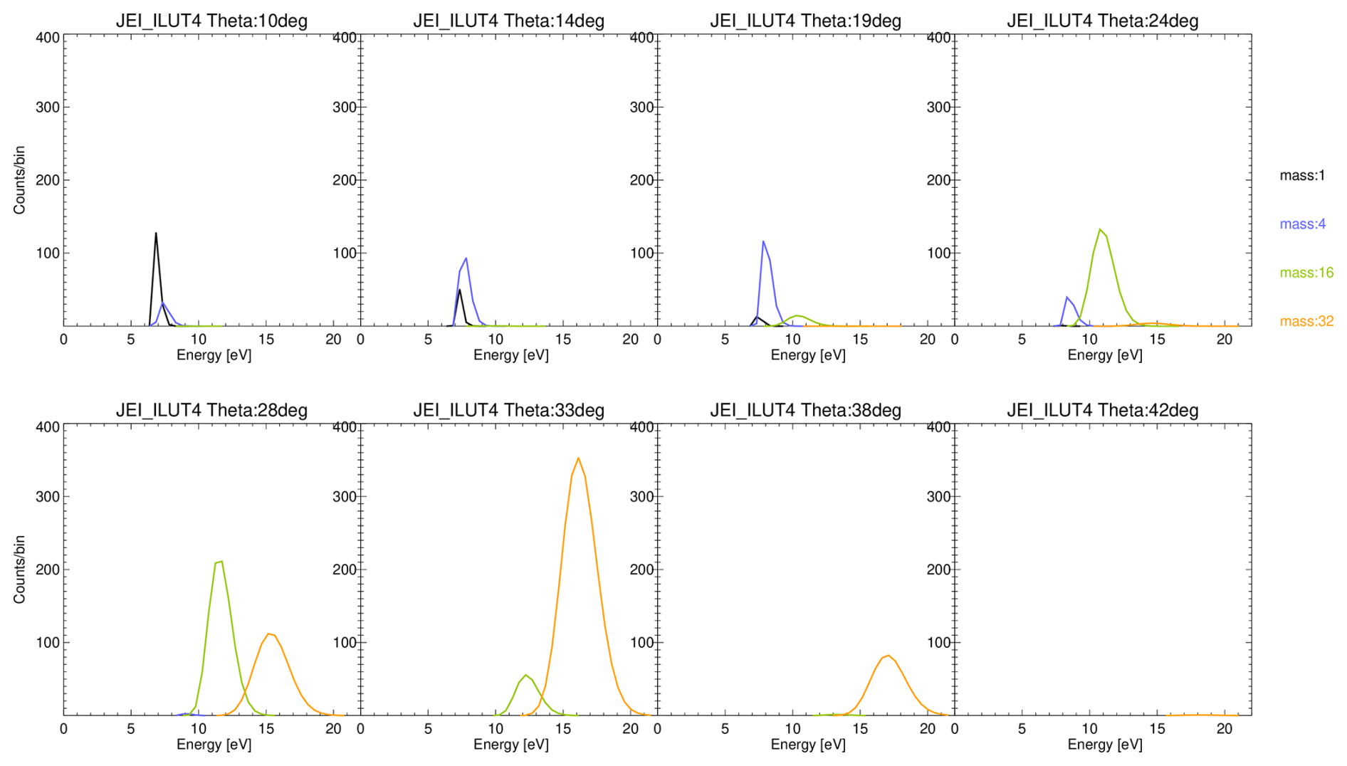
Figure 15 Same simulation setup as in Fig. 14 but with H⁺ CEM efficiency for all ions showing the simulated contribution of different ion species of same density to the observed count spectra for the upper 8 virtual polar angles (listed on top).

The errors shown contain just the error of the counting statistics, but there are several other possible sources of error in these estimations such as: value of spacecraft potential, corotation speed of plasmasphere, polar angle response of the geometric factor, CEM efficiency dependence on mass and energy. Especially the latter may lead to an overestimate of the heavy ion densities. For this reason we repeated the calculation by assuming the efficiency of H⁺ for all ions as shown in Fig. 15. One can see that this makes a significant difference. If we now calculate densities based on this response assumption we get:

$$\begin{array}{}\text{(3)}& \begin{array}{rl}\mathit{\theta }=\mathrm{14}\mathit{°}:n_{{\mathrm{H}}^{+}}& =n_{\mathrm{0}}\times (\mathrm{100.0}\pm \mathrm{10})/\mathrm{90.0}\\ & =\mathrm{1110}\pm \mathrm{110}/{\mathrm{cm}}^{\mathrm{3}},\\ \mathit{\theta }=\mathrm{19}\text{–}\mathrm{24}\mathit{°}:n_{{\mathrm{He}}^{+}}& =n_{\mathrm{0}}\times (\mathrm{80.0}\pm \mathrm{9})/\mathrm{110.0}\\ & =\mathrm{730}\pm \mathrm{80}/{\mathrm{cm}}^{\mathrm{3}},\\ \mathit{\theta }=\mathrm{28}\text{–}\mathrm{33}\mathit{°}:n_{{\mathrm{O}}^{+}}& =n_{\mathrm{0}}\times (\mathrm{65.0}\pm \mathrm{8})/\mathrm{200.0}\\ & =\mathrm{325}\pm \mathrm{40}/{\mathrm{cm}}^{\mathrm{3}},\\ \mathit{\theta }=\mathrm{28}\text{–}\mathrm{33}\mathit{°}:n_{{\mathrm{O}}_{\mathrm{2}}^{+}}& =n_{\mathrm{0}}\times (\mathrm{60.0}\pm \mathrm{8})/\mathrm{350.0}\\ & =\mathrm{170}\pm \mathrm{23}/{\mathrm{cm}}^{\mathrm{3}}.\end{array}\end{array}$$

This comparison shows the significant influence of the CEM efficiency on the calibration for heavy ions. Unfortunately the JEI sensor operated during the observation with a rather low post-acceleration voltage CEM_head of −250 V which does not provide enough acceleration for heavy ions. The nominal post-acceleration for observations at Jupiter in ion mode is −1000 V but for safety reasons this was not applied during the JEI operations during the LEGA. To solidify the quantitative density estimates for these observations laboratory tests of the CEM efficiency at −250 V post-acceleration are needed. In 2017 ion beam tests of the JEI CEMs were done at −370 V total ion energy with ${\mathrm{H}}_{\mathrm{2}}^{+}$ and ${\mathrm{N}}_{\mathrm{2}}^{+}$ ions. These showed that the efficiency of the heavier ions was smaller than for the light ions by a factor of only ∼ 0.8 (Istvan Szemerey, personal communication, 2026). The respective ratio for this energy returned by the MCP formula of Krems et al. (2005) is ∼ 0.1. This indicates that the assumption of a mass independent efficiency can be more realistic for the JEI CEMs. In addition to these considerations a specific correction of the observed densities taking into account the shape of the spacecraft potential may be applied as explained in Appendix D. But this correction is expected to be small compared to the influence of the CEM efficiency.

Nevertheless the simulation results (Eq. 3) show that the heavy ion contribution (O⁺ and ${\mathrm{O}}_{\mathrm{2}}^{+}$) to the total density during the JUICE plasmasphere passage is at least 25 %. Additionally, the spectral peak at 15 eV q⁻¹ is difficult to explain without considering molecular heavy ions.

4 Discussion

The negative charging of the JUICE spacecraft allowed a rare direct measurement of the plasmaspheric cold ion distribution by the PEP JEI electrostatic analyzer. This is a novel measurement as compared to the multiple observations by RPA instruments flown in the earlier phases of magnetospheric science. The advantage of the electrostatic analyzer is a rather high energy and spatial resolution as compared to RPA instruments. More recent missions (Cluster, MMS, Van-Allen-Probe) used electrostatic analyzers but were inhibited by tuning of the instruments to higher energies or by positive charging of the spacecraft. The PEP JEI sensor is a pure energy analyzer and has no built-in mass discrimination. As we have demonstrated above the high spatial resolution of the sensor allows to use the negative spacecraft potential as a mass filter for cold ions when they have a common bulk speed determined by the spacecraft velocity. The location of the flux peak for H⁺ and He⁺ are with 5.2 and 5.6 eV lower than expected for a spacecraft potential of −6.5 V as measured by RPWI. The reason may either lie in a difference between spacecraft ground and JEI electronics ground or a potential deviation at the specific location of the JEI sensor (Zeroual et al., 2026). In our calculations we assume a value of −5.0 V for the potential.

Coming back to the statistical occurrence rate of the spectral peaks with energies above 10 eV q⁻¹ we mentioned above that this type of spectrum was only observed on 28 out of 108 polar scans obtained during the plasmasphere passage. If we assume that the plasmaspheric composition did not change significantly during this 9 min interval the reason for not observing the peaks on every scan must be the narrow polar field of view of only about 5° for a mono-directional beam. Since the 80° polar field-of-view is stepped through in only 8 steps the instrument frequently misses the heavy ion part of the plasma distribution. This effect can be estimated from Fig. 13 when considering that only every second polar sector shown in the Figure is actually observed.

One topic we have not yet discussed is the influence of the magnetic field on the observations. Observations in the outer plasmasphere (L > 3 R_E) indicate in addition to the cold ion distribution a significant warm ion distribution with temperature > 1 eV and mean energy > 10 eV (Goldstein et al., 2023). Unfortunately at the time of writing no offset-corrected magnetic field data are available from the JUICE magnetometers. For this reason we have included in Figs. 6 and 7 only the predicted magnetic field vector from the Tsyganenko96 model. As shown in Fig. 6 the predicted vector is perpendicular to the spacecraft velocity vector. A field parallel acceleration could in principle be explained by a strong electron density gradient (polar wind effect). But the observed distribution is not field parallel and any such acceleration mechanism would create a power law spectral shape (Horwitz et al., 1982) and not the observed cut-off at 15 eV. It can also not explain the peaks in the spectrum which coincide with the modeled location for the different ion masses. Also the azimuthal angle ϕ of the predicted magnetic field is at 90° (Fig. 7), while the observed azimuth is in the range −20 to +20°.

The flux peak observed in the energy spectrum around 15 eV (Fig. 11) indicates the presence of heavy molecular ions in the mass range 30–32 amu q⁻¹. The steep fall off above 15 eV indicates that no heavier molecules than mass 32 amu q⁻¹ are present. Since the efficiency of the JEI CEMs at the very low post-acceleration voltage of −250 V is not well known further calibrations are needed to quantify the relative contributions of the different ion species to the observed spectra.

The observed ion temperatures (Fig. 10) should in principle not depend on the spacecraft potential when the negative potential is lower than the undisturbed minimum energy for a specific ion species. But this is not the case for the spectra observed at θ = 14.4° and θ = 23.8° where the observed mean energy is very close to the spacecraft potential reported by the RPWI instrument. In this case the part of the spectrum which is lower than the spacecraft potential will be accumulated in a single energy bin and the Maxwellian fit in energy space results in too low temperatures. We discuss this effect in Appendix B with the conclusion that the temperature should only be derived from the upper part of the energy distribution. But this can not explain why the temperature values reported in Fig. 10 are lower than those obtained by earlier measurements using RPA instruments (Kotova et al., 2008).

If we now consider the implications of our analysis for observations by the JUICE spacecraft in the plasma environment of the Jovian moons we first note that a negative spacecraft charging was also observed by the PLS instrument on the Galileo spacecraft (Frank and Paterson, 2000). Bochet et al. (2023) calculated spacecraft potentials for the Ganymede and Jupiter magnetospheric phases of the JUICE mission using the SPIS potential simulation software. For the Ganymede phase they predict a negative potential of −15.5 V at a Debye length of 1.2 m such for this phase the methods described in our analysis may be applied with some modification. For the Jupiter magnetospheric phase Bochet et al. (2023) predict a positive potential of +4 V at a Debye length of 120 m. In this case the common assumption of a spherical potential geometry can be applied.

5 Conclusions

During the first gravity assist of JUICE at Earth on 20 August 2024 the spacecraft passed through the Earth plasmasphere for about 2 h. Before closest approach at a distance of 2.1 R_E the Jovian Electron and Ion spectrometer (JEI) of the PEP instrument suite was switched on for 40 min in an ion mode test configuration. The high plasma density of about 3000/cm³, as observed by the RPWI plasma wave instrument, led to a negative charging of the spacecraft which allowed a rare observation of the cold and dense plasmaspheric ion population. Since the ions are only corotating with the Earth with a velocity of about 1 km s⁻¹ at this distance the observed ion speed is dominated by the spacecraft velocity of about 8 km s⁻¹. For this reason ions with different masses are separating in the energy spectrum observed by JEI. In addition the spacecraft potential leads to specific filtering of ion masses in the observed angular distribution. By calculating the sensor response function for this specific geometry it is possible to quantify densities of the different ion species. This response calculation depends critically on the response of the JEI CEMs to the ion velocity and mass. Since the sensor was operated with a low post-acceleration, further laboratory calibrations may be needed for this specific setup. Still we can already conclude from the observations that ions with mass > 4 amu q⁻¹ contribute at least 25 % to the observed total density. A flux peak observed in the energy spectrum at 15 eV q⁻¹ can only be explained by the presence of heavy molecular ions with mass ∼ 30 amu q⁻¹. Molecular ions have only been rarely detected in the outer Earth plasmasphere. With respect to the performance and operations of PEP JEI, these observations show that PEP JEI can achieve sensitive ion composition measurements in the exospheres of the moons of Jupiter.

Appendix A: JEI sensor properties

Table A1 General properties of the PEP JEI sensor. Performance parameters will be updated during the JUICE inflight calibration campaign.

Appendix B: The PEP JEI particle distribution function

The PEP JEI sensor is an electro-static particle analyzer using electro-static deflectors (Barabash and PEP-team, 2026; Bambach, 2026). This means at a given time step τ_s (= 4 ms in the case discussed here) the sensor counts ions or electrons with a specific mean energy E_m and energy distribution with a FWHM ΔE coming from a specific polar direction θ with a polar FWHM Δθ ≈ 5°. The actual energy and polar width are dependent on θ (see Bambach, 2026).

JEI sweeps the energy analyzer and deflector voltages in parallel in 128 steps such that one energy spectrum is obtained within 512 ms from a specific polar direction θ. The polar hemisphere is stepped through by 8 polar steps in the range 10 to 75° measured from the sensor symmetry axis. This means specifically for cold plasma distributions polar directions between each polar step may not be covered in this operation mode. The azimuth field of view is sampled simultaneously by the 16 anodes of the sensor. But since efficiency and noise background of each anode are different we here consider only one specific azimuth sector ϕ with its width Δϕ. In summary the sensor samples counts $c(E,\mathit{\varphi },\mathit{\theta })$ from a specific viewing direction at a given time within the sampling period $\mathit{\tau }={\mathit{\tau }}_{\mathrm{s}}-d$, where d = 1 ms is the dead time between each energy step. The differential energy flux can be obtained from the count rate by (Fränz et al., 2006):

$$\begin{array}{}\text{(B1)}& J_{\mathrm{E}}(E,\mathit{\varphi },\mathit{\theta })={\displaystyle \frac{c(E,\mathit{\varphi },\mathit{\theta })}{G_{\mathrm{E}}\mathit{\tau }}}\end{array}$$

where G_E is the energy geometric factor which is assumed to be constant over the low energy interval under discussion. The partial phase space density for a given plasma component with mass m and velocity v is then given by

$$\begin{array}{}\text{(B2)}& f\left(\mathit{v}\right)={\displaystyle \frac{m^{\mathrm{2}}\cdot J_{\mathrm{E}}(E,\mathit{\varphi },\mathit{\theta })}{\mathrm{2}{E}^{\mathrm{2}}}}\end{array}$$

where $\mathit{v}=\sqrt{\mathrm{2}E/m}\cdot \mathit{n}$ and $\mathit{n}=(\sin \mathit{\theta }\cos \mathit{\varphi },\sin \mathit{\theta }\sin \mathit{\varphi },\cos \mathit{\theta })$ is the vector opposite to the viewing direction.

The energy geometric factor of JEI for an isotropic distribution is given in Table A1. The factor is larger for a mono-directional flow when looking into flow direction and needs to be modeled for each case.

Appendix C: A drifting Maxwellian distribution in a planar potential

To derive the expected energy flux for a given drifting Maxwellian plasma flow with density n, mean velocity $\stackrel{\mathrm{‾}}{\mathit{v}}$ and thermal velocity v_t we can use its phase space density distribution in the observation frame:

$$\begin{array}{}\text{(C1)}& f\left(\mathit{v}\right)={\displaystyle \frac{n}{(\sqrt{\mathit{\pi }}{v}_{\mathrm{t}}{)}^{\mathrm{3}}}}\cdot \exp \left[-{\displaystyle \frac{(\stackrel{\mathrm{‾}}{\mathit{v}}-\mathit{v}{)}^{\mathrm{2}}}{v_{\mathrm{t}}^{\mathrm{2}}}}\right]\end{array}$$

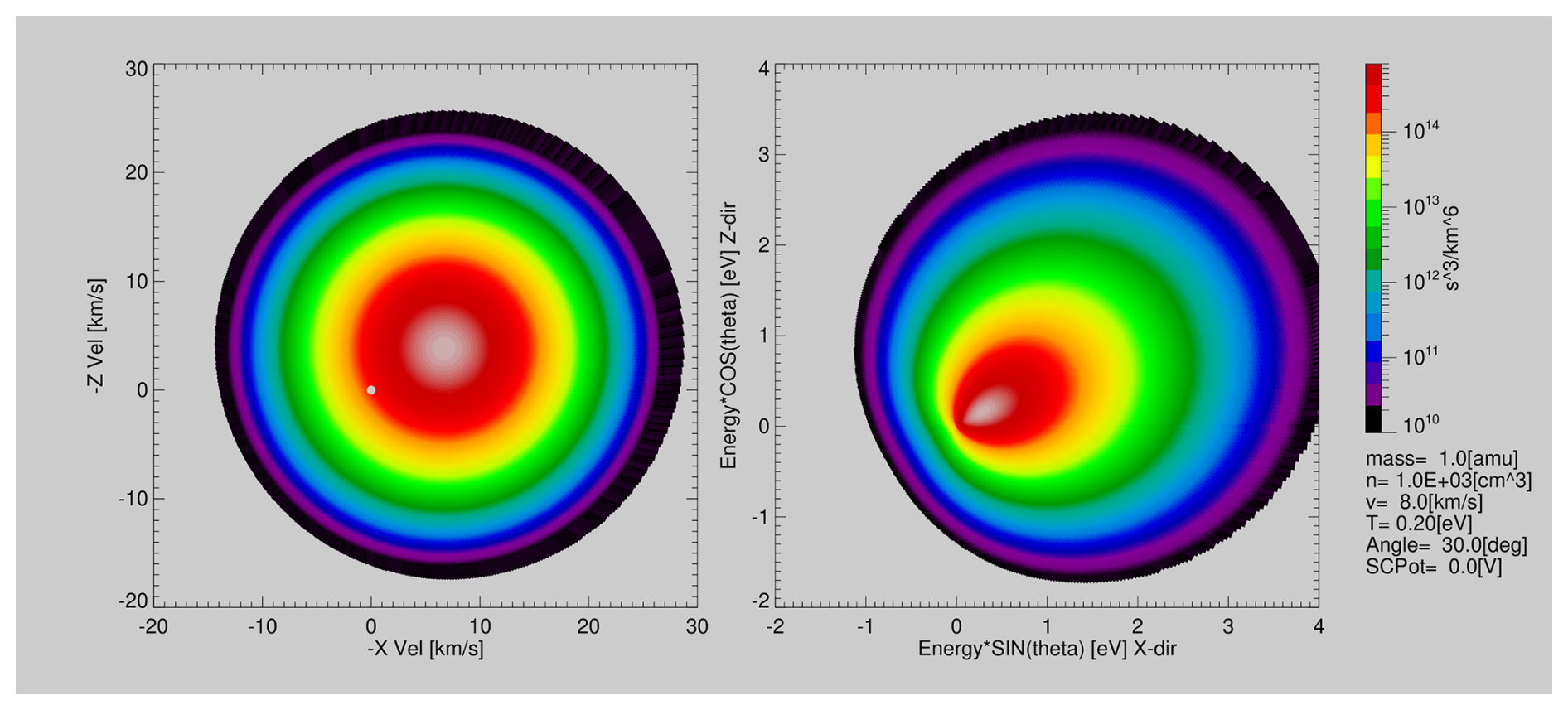
Figure C1 Phase space distribution in velocity space (left) and energy space (right) of a Maxwellian proton distribution of thermal temperature 0.2 eV and density 1000/cm³ drifting with velocity 8.0 km s⁻¹ at an angle of θ_D = 40° with respect to the X-axis and zero spacecraft potential. Shown is the cut through the v_z = 0 plane with inverted velocity signs. The dot at coordinate (0,0) is an artifact of the energy table used.

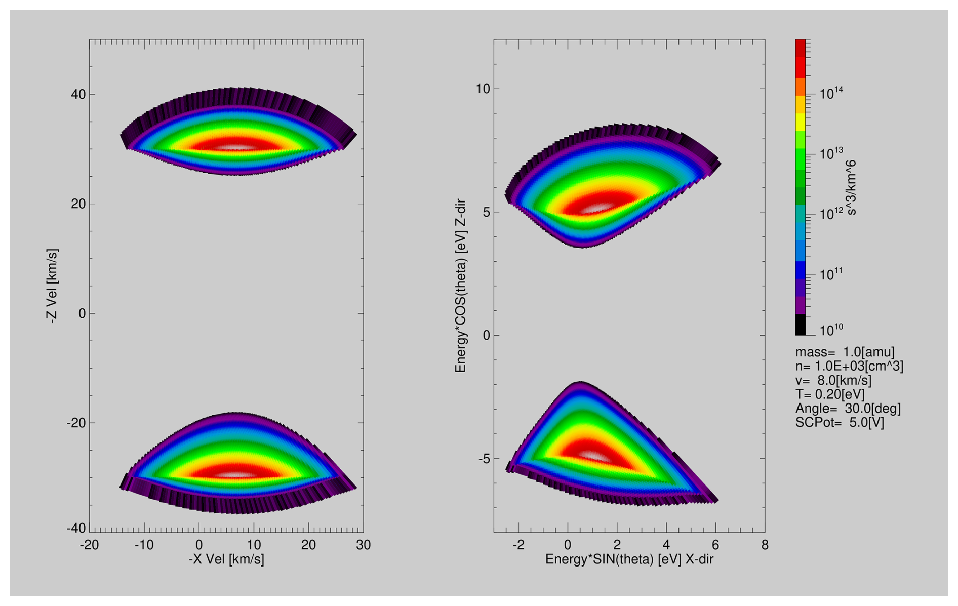
Figure C2 Same as Fig. C1 but with a planar vertical spacecraft potential of −5.0 V added. The upper half of the distribution as seen from the +Z deck of the spacecraft, the lower half as seen from the -Z deck of the spacecraft.

The respective phase space distribution is illustrated in Fig. C1 for observation conditions similar to those described in the text. The observation plane (spacecraft nadir deck) can be thought off as the plane given by v_z = 0, that is the part of the distribution with v_z < 0 is not observed by a sensor on the deck.

While the flow is mono-directional the observation geometry of the sensor is spherical. To use spherical coordinates we can express the vector coordinates by

$$\begin{array}{}\text{(C2)}& \begin{array}{rl}f(v,\mathit{\theta },\mathit{\varphi })=& {\displaystyle \frac{n}{(\sqrt{\mathit{\pi }}{v}_{\mathrm{t}}{)}^{\mathrm{3}}}}\\ & \times \exp \left[-{\displaystyle \frac{{\stackrel{\mathrm{‾}}{v}}^{\mathrm{2}}-\mathrm{2}\stackrel{\mathrm{‾}}{v}\left|v\right|\cos \mathrm{\Delta }\mathit{\sigma }+v^{\mathrm{2}}}{v_{\mathrm{t}}^{\mathrm{2}}}}\right]\end{array}\end{array}$$

where Δσ is the distance between viewing direction (ϕ,θ) and mean flow direction (ϕ_f,θ_f) along the great circle (all angles in radian):

$$\begin{array}{}\text{(C3)}& \mathrm{\Delta }\mathit{\sigma }=\arccos (\cos \mathit{\theta }\cos {\mathit{\theta }}_{\mathrm{f}}+\sin \mathit{\theta }\sin {\mathit{\theta }}_{\mathrm{f}}\cos |\mathit{\varphi }-{\mathit{\varphi }}_f\left|\right)\end{array}$$

The sensor measures energy spectra in different spatial directions. To compare with the observations we replace the thermal velocity v_t by thermal energy E_t, the mean velocity by mean energy $\stackrel{\mathrm{‾}}{E}$ and the total of the velocity by the respective energy and get

$$\begin{array}{}\text{(C4)}& \begin{array}{rl}f(E,\mathit{\theta },\mathit{\varphi })=& n\cdot {\left({\displaystyle \frac{m}{\mathit{\pi }\mathrm{2}{E}_{\mathrm{t}}}}\right)}^{\mathrm{3}/\mathrm{2}}\\ & \times \exp \left[-{\displaystyle \frac{\stackrel{\mathrm{‾}}{E}-\mathrm{2}\sqrt{\stackrel{\mathrm{‾}}{E}E}\cos \mathrm{\Delta }\mathit{\sigma }+E}{E_{\mathrm{t}}}}\right].\end{array}\end{array}$$

This generalizes Eq. (18) of Fränz et al. (2006) which is only valid for Δσ = 0 and is illustrated in Fig. C1.

If we just consider an anode looking in flow direction (that is receiving the peak signal) we can assume ϕ=ϕ_f. In this case we get

$$\begin{array}{}\text{(C5)}& \cos \mathrm{\Delta }\mathit{\sigma }=\sin \mathit{\theta }\sin {\mathit{\theta }}_{\mathrm{f}}+\cos \mathit{\theta }\cos {\mathit{\theta }}_{\mathrm{f}}=\cos (\mathit{\theta }-{\mathit{\theta }}_{\mathrm{f}})\end{array}$$

Using Eqs. (C1) and (C4) we can thus determine for an assumed Maxwellian plasma flow the expected energy flux in each angular direction and energy bin of the sensor.

The effect of a potential distribution on a drifting Maxwellian distribution was first described in the seminal paper by Mott-Smith and Langmuir (1926) in the context of laboratory plasma probes. But in this study it was not explicitly formulated for the planar geometry case. More recent discussions can be found in Génot and Schwartz (2004) and Štverák et al. (2026) for spherical geometries.

If we now introduce a planar spacecraft potential located in the z=0 plane the observed velocity distribution is only affected in the v_z=vcos θ coordinate. We use the thin-sheath approximation (Whipple et al., 1974) which neglects effects on ions which initially are inside the volume affected by the potential. The temperature of the distribution E_t given in the exponent of the equations above is not directly affected by this, but the phase space distribution in the observed velocity space is shifted such that the observed velocity and energy are

$$\begin{array}{}\text{(C6)}& \begin{array}{rl}{v}_{\text{zp}}& =\sqrt{-\mathrm{2}q{V}_{\mathrm{p}}/m-v^{\mathrm{2}}\left|\cos \mathit{\theta }\right|\cos \mathit{\theta }}\\ E_{\mathrm{p}}& =E\cdot (\mathrm{1}-{\cos }^{\mathrm{2}}\mathit{\theta }-|\cos \mathit{\theta }\left|\cos \mathit{\theta }\right)-q{V}_{\mathrm{p}}\text{ or:}\\ E_{\mathrm{p}}& =E-q{V}_{\mathrm{p}}\text{ for }\mathit{\theta }>\mathit{\pi }/\mathrm{2}\\ E_{\mathrm{p}}& =E\cdot (\mathrm{1}-\mathrm{2}{\cos }^{\mathrm{2}}\mathit{\theta })-q{V}_{\mathrm{p}}\text{ for }\mathit{\theta }<\mathit{\pi }/\mathrm{2}.\end{array}\end{array}$$

where θ is the undisturbed angle from the v_z axis and V_p<0. That means ions which initially have negative v_z (that is flying towards the Z=0 deck) gain the full energy −qV_p, ions with initially positive v_z are decelerated, but are still observed as long as E_p>0. The observed angle θ_p is given by Eq. (1). This separation of the distribution into accelerated and decelerated ions was missed in the treatment of the problem by Štverák et al. (2026). When integrating the phase space distribution one also needs to consider the transformation of the volume element $\mathrm{dV}=v^{\mathrm{2}}\sin \mathit{\theta }\mathrm{dv}d\mathit{\theta }d\mathit{\varphi }=\sqrt{\frac{\mathrm{2}E}{m^{\mathrm{3}}}}\mathrm{dE}\sin \mathit{\theta }d\mathit{\theta }d\mathit{\varphi }$. The respective distribution in energy space is illustrated in Fig. C2.

For completeness we also show in Fig. C2 the phase space distribution which would be observed on the opposite side of the spacecraft for the same drifting Maxwellian and −5.0 V spacecraft potential attracting ions towards the +Z direction. This situation is relevant for the PEP JDC sensor which is mounted on the opposite deck of the spacecraft. The respective synchronous observations of this sensor are described in an accompanying paper.

Interesting for the analysis of an energy spectrum f(E_p) observed at a specific angle θ_p is how to derive temperature, potential and mean energy from the spectrum. Since the spectrum is distorted for $\mathit{\theta }<\mathit{\pi }/\mathrm{2}$ one may derive temperature from a fit to the upper leg of the distribution. The question is at which value of E_p the maximum phase space density is observed. This is the case when $\frac{df\left(E\right)}{\mathrm{dE}}=\mathrm{0}$. From Eq. (C4) we get

$$\begin{array}{}\text{(C7)}& \begin{array}{rl}{\displaystyle \frac{df\left(E\right)}{\mathrm{dE}}}=& -{\displaystyle \frac{f\left(E\right)}{E_{\mathrm{t}}}}{\displaystyle \frac{d}{\mathrm{dE}}}\left(\stackrel{\mathrm{‾}}{E}-\mathrm{2}\sqrt{\stackrel{\mathrm{‾}}{E}E}\cos \mathrm{\Delta }\mathit{\sigma }+E\right)\\ & ⟹\sqrt{\stackrel{\mathrm{‾}}{E}/E_{\mathrm{m}}}\cos \mathrm{\Delta }\mathit{\sigma }+\mathrm{1}=\mathrm{0}\\ & ⟹E_{\mathrm{m}}=\stackrel{\mathrm{‾}}{E}{\cos }^{\mathrm{2}}\mathrm{\Delta }\mathit{\sigma }\end{array}\end{array}$$

For $\mathit{\theta }>\mathit{\pi }/\mathrm{2}$ this means the maximum observed phase space density is at $E_{\text{pm}}=q{V}_{\mathrm{p}}+\stackrel{\mathrm{‾}}{E}{\cos }^{\mathrm{2}}\mathrm{\Delta }\mathit{\sigma }$ which will allow to derive V_p for known drift velocity $\stackrel{\mathrm{‾}}{v}$ and angle Δσ. For a Maxwellian distribution at rest the observed width of the distribution in each spatial direction is given by E_t. If we define the energy E_e at which the distribution falls off by $\mathrm{1}/e$ through $f\left(E_{\mathrm{e}}\right)=f\left(E_{\mathrm{m}}\right)/e$, we get for the drifting Maxwellian:

$$\begin{array}{}\text{(C8)}& E_{\mathrm{e}}=\stackrel{\mathrm{‾}}{E}{\cos }^{\mathrm{2}}\mathrm{\Delta }\mathit{\sigma }+E_{\mathrm{t}}\pm \mathrm{2}\cos \mathrm{\Delta }\mathit{\sigma }\sqrt{\stackrel{\mathrm{‾}}{E}{E}_{\mathrm{t}}}\end{array}$$

The width of the distribution is then $E_{\mathrm{w}}=E_{\mathrm{e}}-E_{\mathrm{m}}=E_{\mathrm{t}}\pm \mathrm{2}\cos \mathrm{\Delta }\mathit{\sigma }\sqrt{\stackrel{\mathrm{‾}}{E}{E}_{\mathrm{t}}}$. That means only perpendicular to the flow direction (cos Δσ=0) the observed temperature agrees with the real temperature E_t.

Appendix D: Density correction in a planar potential

The effect of electric potentials on the plasma flow was already analyzed in much detail in the seminal paper by Mott-Smith and Langmuir (1926) in the context of plasma probes. For convenience in the following we describe the derivation in planar geometry since the more recent papers usually assume spherical geometry (Lavraud and Larson, 2016). We generally assume that the spacecraft is located in a mono-directional plasma flow with density n₀ and velocity v₀. If the ion sensor is located behind a planar entrance grid and the flow is perpendicular to this grid we are dealing with a one-dimensional problem as shown in Fig. D1. Liouville's theorem in general form states that the phase space density of particles $S=\mathrm{dN}/\mathrm{dV}$ in a volume element dV of phase space is conserved along the flow, in cartesian geometry:

$$\begin{array}{}\text{(D1)}& S{\mathrm{dv}}_x{\mathrm{dv}}_y{\mathrm{dv}}_z\mathrm{dx}\mathrm{dy}\mathrm{dz}=\mathrm{dN}\end{array}$$

where dN denotes the number of particles and dV=dv_xdv_ydv_zdxdydz the size of the volume element. In 1D geometry this reduces to $\frac{\mathrm{dN}}{\mathrm{dv}\mathrm{dx}}=\text{constant}$ since dv_ydv_zdydz is constant. Now, the quantity measured by ion sensors is the flux of ions F with mean energy E crossing an area dA perpendicular to the flow direction in a given time dt for a given energy interval dE. In 1D the spatial extent of the volume element along the flow is given by dx=vdt and since dE=vdv we have

$$\begin{array}{}\text{(D2)}& S\mathrm{dv}\mathrm{dx}=S{\displaystyle \frac{\mathrm{dE}}{v}}v\mathrm{dt}=S\mathrm{dE}\mathrm{dt}\propto \mathrm{dN}\end{array}$$

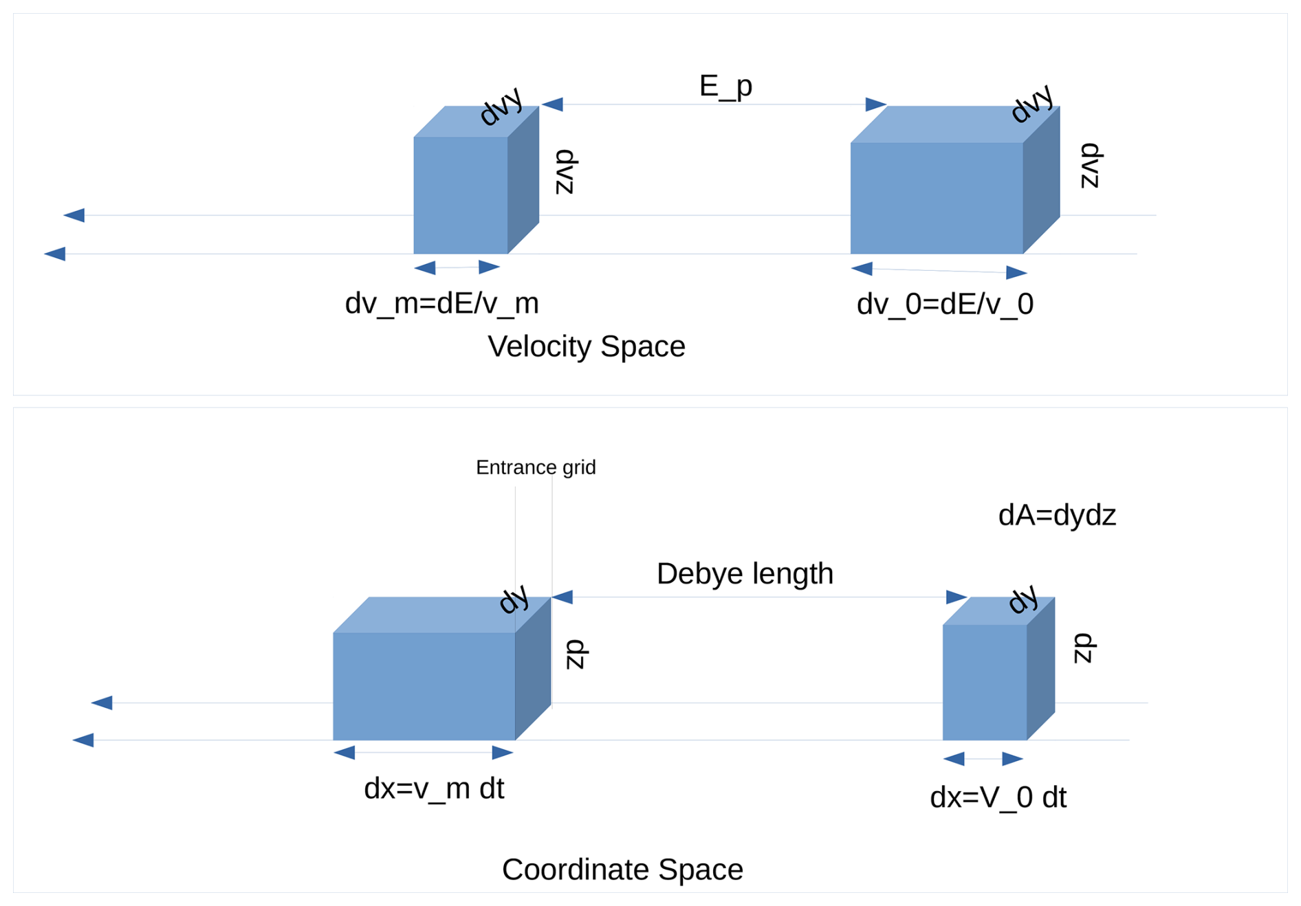
Figure D1 Planar geometry of acceleration by potential in velocity and coordinate space. The size of the phase space volume element does not change. Flux through surface dA is conserved.

The particle number flux of particles crossing a given area dA in a given time dt is given by $F=\mathrm{dN}/\mathrm{dA}\mathrm{dt}\sim S\mathrm{dE}$. Liouville's theorem in 1D then states $F/\mathrm{dE}$ is constant. Thus if an instrument measures with the same energy width dE outside of the potential or inside of the potential it will measure the same particle number flux – only at a different energy. From $E_{\mathrm{m}}=E_{\mathrm{0}}+E_{\mathrm{p}}$ it follows also that dE_m=dE₀. Here we also make the same assumption as Mott-Smith and Langmuir (1926) namely that all ions are accelerated by the same energy per charge after they enter the volume affected by the potential. This is also called thin-shield approximation (Whipple et al., 1974).

We again stress that if a sensor measures with a geometric factor which depends on energy it is irrelevant for this discussion because this happens behind the entrance grid of the sensor. Outside of the potential the number flux is given by F=n₀v₀, since the mean velocity v_m measured inside of a potential E_p is given by $v_{\mathrm{m}}=\sqrt{v_{\mathrm{0}}^{\mathrm{2}}+s{v}_{\mathrm{p}}^{\mathrm{2}}}$, where $v_{\mathrm{p}}=\sqrt{\mathrm{2}\left|E_{\mathrm{p}}\right|/m}$ and $s=-\text{sign}\left(E_{\mathrm{p}}\right)$, the observed ion density n_m is given by

$$\begin{array}{}\text{(D3)}& n_{\mathrm{m}}={\displaystyle \frac{n_{\mathrm{0}}{v}_{\mathrm{0}}}{\sqrt{v_{\mathrm{0}}+s{v}_{\mathrm{p}}}}}={\displaystyle \frac{n_{\mathrm{0}}}{\sqrt{\mathrm{1}+s{\left(\frac{v_{\mathrm{p}}}{v_{\mathrm{0}}}\right)}^{\mathrm{2}}}}}={\displaystyle \frac{n_{\mathrm{0}}}{R_{\mathrm{v}}}}\end{array}$$

where we define the velocity ratio $R_{\mathrm{v}}=\sqrt{\mathrm{1}+s(\frac{v_{\mathrm{p}}}{v_{\mathrm{0}}}{)}^{\mathrm{2}}}$. That means the observed density is lower than the undisturbed density n₀ for a negative potential. We note that this is different from the usual correction for potentials with a spherical geometry where the potential focuses the flux (Lavraud and Larson, 2016).

But there is one assumption in this derivation which may not be applicable for actual measurement situations, namely that always all particles flying through the volume element backward and forward are measured. In reality only the part of a distribution flying towards a sensor are measured. As shown in the previous section this means for example for an undisturbed Maxwellian distribution and a given one dimensional look direction only half of the distribution is observed. When an attracting potential is added a larger part of the distribution becomes visible in this look direction and lost from the opposite direction. In the Liouville picture also particles flying in opposite direction are included in dN.