Incoherent Scatter Radar Observations of the F Region of the Ionosphere above the Eastern US during the April 2024 Solar Eclipse

We present dynamic mid-latitude ionospheric changes associated with the 8 April 2024 solar eclipse, as observed in the eastern to central United States using wide-field scans from the Millstone Hill incoherent scatter radar. The radar's field of view covers a large portion of the continental US (25–55° N, 75–95° W), and is capable of observing altitude profiles from the E-region up to the topside ionosphere. We find that extensive ionospheric changes triggered by the eclipse along the US east coast began as early as when the penumbra shadow makes contact with the scanning region or when the eclipse obscuration percentage exceeds 0 %. During the time interval where the obscuration percentage is significant (>75 %) over the radar scanning region, we find maximum electron density (N_e) drops of up to 50 % (2 × 10¹¹ m⁻³) in the F1 region (200–250 km) to the north of the totality path, with a large N_e decrease lasting for 1 h, from 19:00–20:00 UT. In the topside ionosphere, a delayed drop in N_e values occurred beginning 30 min–1 h later, with electron density decreasing by 40 %–50 % (2.5–3 × 10¹¹ m⁻³) below background levels, followed by a recovery to typical background values only after 22:00 UT. The electron temperature (T_e) showed a faster response time and recovery rate which closely mirrored the eclipse obscuration level, with a visible decrease in T_e when the obscuration rate exceeded 0 %–30 % depending on the altitude, with a faster response time with increasing altitude below 300 km, but an approximately flat response time above 300 km altitude. A decrease in T_e of the order of 40 % (850 K) was observed at altitudes from 325–400 km between 18.75–19.25 UT. The ion temperature (T_i), similar to T_e, responded rapidly to the obscuration level as it exceeded 30 %, with up to 20 % or 225 K reduction in a narrow geographic area and at two distinct altitude regions: 200–225 and 300–325 km between 19:00–20:00 UT.

1 Introduction

Solar eclipses present an outstanding opportunity to observe variations in the near-Earth space environment in response to rapid changes in solar extreme ultraviolet (EUV) radiation. The dynamic physical response to eclipse-associated perturbations can serve as unique experiments that test our knowledge of thermosphere-ionosphere coupling processes. Each solar eclipse offers a distinctly different opportunity, as it occurs during a different season, local time, and level of solar activity, and traverses a different geographic region. Hundreds of research papers have been devoted to understanding the response of the ionosphere-thermosphere system to solar eclipses, starting from events as early as the 1920s during the first decades of ionospheric observation (Ratcliffe, 1956). A brief historic perspective on eclipse studies is described by Bravo et al. (2020), and an interested reader is referred to references therein. In general, during a solar eclipse Earth's moon temporarily blocks solar ionizing EUV radiation, resulting in decreases in ionospheric electron density and electron temperature. As ionospheric plasma and the neutral thermosphere are closely coupled due to dynamic and electrodynamic processes (e.g. ion-neutral collisions), eclipse-induced perturbations from an initial background state can occur in multiple neutral and plasma parameters, including neutral temperature, composition, wind, electric field, plasma temperature, and plasma density. Detailed observations of perturbations during solar eclipses provide an excellent opportunity to investigate the mechanisms of ion-neutral coupling and improve our knowledge of thermal, photochemical, and electrodynamic processes in the near-Earth space environment.

On 8 April 2024, a total solar eclipse occurred over North America, moving from the southern portion of the continent (Mexico) to the north-eastern portion (Canada). The continental portion of United States experienced eclipse conditions from ∼ 17:00 to 21:00 UT. Aa et al. (2024) used multi-instrument observations and data assimilation to investigate a 3D evolution of mid-latitude electron density during the eclipse. They concluded that ionospheric electron density decreased by 20 %–50 % near the totality area, maximum depletion occurred near 200–250 km altitude, and eclipse response in the topside ionosphere peaked at 1–2.5 h after the time of peak obscuration. Zhang et al. (2024) also used multi-instrument observations and concluded that maximum depletion in total electron content (TEC) was observed with a 14–23 min delay from the time of maximum obscuration. That study also described TEC decrease by ∼ 10 TECu, and a significant peak electron density N_mF2 decrease by 40 %–70 %. Kunduri et al. (2024) used SuperDARN HF radar observations and found a ∼ 45 min delay between maximum obscuration time and a maximum effect on HF refractive skip distance, related to the delayed change in F-region electron density. They also suggested that the neutral thermosphere likely played an important role in the observed variations in plasma density. Yang et al. (2025)'s study concluded that reduction in TEC during this eclipse exceeded 15 TECu, and N_e decreased by ∼ 30 % below 250 km and by ∼ 60 % above 250 km. Le et al. (2025) estimated that TEC decreased by 20 %–40 %, and maximum electron density decreased by ∼ 30 % near 300 km altitude. Chernogor and Holub (2025) investigated variations in the geomagnetic field during eclipse passage, finding perturbations of the order of 10 nT in all components of the geomagnetic field. Most of these available studies addressed eclipse-induced variations in electron density because of the abundance of electron density data, with differences in the reported strength and timing of the plasma density response explained using different methods of obtaining reference ionosphere and/or proximity of specific observation to the maximum obscuration zone.

This study extends knowledge of ionospheric eclipse response by exploring the spatial and temporal variations in the ionospheric response to the 8 April 2024 solar eclipse using observations of multiple ionospheric parameters (electron density N_e, electron temperature T_e, ion temperature T_i) collected by the Millstone Hill incoherent scatter (IS) radar. The main goals of the study are (1) to accurately identify eclipse-induced variations in N_e, T_e, T_i over central to eastern North America, and (2) to discuss observed features that challenge current understanding of ionosphere-thermosphere coupling processes. To separate eclipse-induced variations, we construct an empirical model of ionospheric parameters encompassing both historic IS radar observations and observations collected in April 2024. As Millstone Hill scanned North America over a broad range of latitudes and longitudes (75–95° W and ∼ 25–55° N), the resulting combination of spatio-temporal features and observations of ionospheric state variations in multiple parameters (N_e, T_e, T_i) produces a unique observational perspective not available from other studies. In particular, the IS radar technique is the only available method which directly produces ionospheric plasma temperature as an incisive diagnostic.

This report is organized as follows. Section 2 describes the setup of observations used in this study and the main features of the background empirical ionospheric model. Section 3 presents results in terms of absolute and relative (percentage difference) changes in N_e, T_e, T_i due to the solar eclipse. Section 4 discusses observed features in the context of previous observations and current knowledge about ionosphere-thermosphere connections. The summary of the main results and conclusions are given in Sect. 5.

2 Methods

We utilize data from the high power large aperture UHF Millstone Hill incoherent scatter radar and its 46 m diameter Magnetosphere-Ionosphere Steerable Antenna (MISA), operated as part of MIT Haystack Observatory's Millstone Hill Geospace Facility and located in Westford, Massachusetts at 42.6° N, 71.5° W. The fully steerable MISA antenna was originally installed at the Sagamore Hill Air Force facility in Wenham, Massachusetts, in 1963, and was moved to Millstone Hill in 1978. The MISA is used primarily as a UHF radar antenna combined with a megawatt class transmitter for measurements of the near-space environment using the incoherent scatter radar technique. For this study, we used MISA data from wide field 6° elevation scans, utilizing a 2 ms uncoded transmitted pulse. The low elevation nature of the radar scan, combined with the hilltop view available at MIT Haystack, allows observation with a geographic spread that encompasses a large portion of the eastern US, stretching in geodetic latitude from 25–55° N and in longitude from 75–95° W. This class of low elevation and wide coverage scanning experiments have been extensively used over decades for geospace stormtime dynamics investigations, as shown in (Zhang et al., 2017; Aa et al., 2020) along with a number of other studies at Millstone Hill.

The radar experiment observation sequence consisted of two modes. Mode 1 employed a counterclockwise MISA scan at 6° elevation, progressing in azimuth from ∼ −43 to ∼ −145° (where 0° = geographic north). The total scan duration of 15 min was divided into 21 individually processed subscan intervals of ∼ 45 s integrations. Each radar scan was followed by a 15 min regional ionospheric observation sequence (Mode 2). Mode 2 consisted of vertical/zenith profile measurements combined with two fixed position MISA measurements at 45° elevation for determination of scalar and vector ionospheric E and F region parameters in a cone approximately 2° latitude/longitude around Millstone Hill. This study concentrates on Mode 1's wide field observations of mid latitude ionospheric dynamics.

MISA ion-acoustic power spectral data is processed to obtain ionospheric plasma parameters using the production level Millstone Hill analysis chain. Ion-acoustic power spectra are generated by the MIDAS-W standard software based radar signal processing chain with trapezoidal summation rules used to produce each altitude's power spectral density estimate (Grydeland et al., 2005). Subsequently, using standard incoherent scatter theory forward models (Kudeki and Milla, 2011), a Levenberg-Marquardt based iterative nonlinear least squares fitting process incorporates radar ambiguity functions in the forward model that take into account waveform based averaging effects for uncoded pulses as well as effective receiver bandwidths and other frequency-dependent spectral effects. In addition, altitude profiles of electron density are obtained from collective Thomson/incoherent scatter radar theory (Evans, 1969) using a volumetric target radar equation, including a term connecting radar signal power to electron density through a calibration factor. This calibration constant is determined by direct comparison of measurements of signal power from the F-region electron density peak with plasma line/Langmuir mode measurements of peak electron density. Measurement of the plasma line return (frequency of scattered energy) at the F region peak directly connects electron density to fundamental physical constants. Since a frequency is measured as opposed to an area under a curve, accuracy of the resulting plasma line derived electron density is well under 1 %. Electron density has been routinely calibrated at Millstone Hill using the plasma line technique since 1 January 2016. Descriptions can be found, for example, in Shammat et al. (2024), with the study describing the overall calibration procedure. Numerous other studies utilized Millstone Hill ISR plasma line calibrated data (Wang et al., 2019, Fig. 2, during the 2017 solar eclipse; Zhang et al., 2019, Fig. 14, during a solar flare; Zhang et al., 2021a, two traveling ionospheric disturbances events). The above processing yields final calibrated estimates of electron density (N_e), electron temperature (T_e), and ion temperature (T_i) parameters as a function of altitude, including quantified uncertainties. Effective altitude resolution in the Mode 1 analyzed results is between 22 and 32 km in the ionospheric F region and near topside, with along-beam horizontal averaging of 0.3 to 0.5° in latitude/longitude in the same altitude region. Because of the use of a 2 ms long pulse at low elevation, the horizontal resolution of the variations resolved by the radar is unavoidably larger than 300 km, and any ionospheric variation within the pulse length is averaged. Therefore, the study analysis focuses on the comparisons of large scale ionospheric variations such as across the broad areas of the near topside and the F region or over large longitudinal spans.

Figure 1 (upper panel) visually illustrates the geometry of a Mode 1 6° elevation 3D MISA elevation scan, and the 2D projection of the scan (lower panel) on the latitude-longitude plane. The 2D projection shows the azimuth angles of the scanning positions on 8 April 2024. The center of the main beam during each Mode 1 scan occurs along the azimuths labeled in red in the bottom panel of the figure starting at −43° and ending at −143° over a period of 15 min. The eclipse totality path, shown with a semi-transparent blue color, cuts across the flattened scanning region and overlaps azimuths between −88 to −103° as it moves northeastward. Note that for several consecutive scans during the experiment, a significant portion of the scanning region experiences 70 %–100 % obscuration.

In Figs. 3 and 4, we present the experimental uncertainties of the Millstone Hill steerable 46 m antenna 6° elevation 2 ms long uncoded pulse mode data. Figure 3 shows the uncertainties associated with each of the parameters (N_e, T_e, and T_i) for a single azimuth ∼ −93° over range profiles (shown in altitude measurements) on 8 April 2024. Each of the panels shows the profiles 2 h before maximum obscuration over the scanning region, during maximum obscuration over the scanning region, and 2 h after maximum obscuration. As we can see, errors associated with measurements from 200–400 km are low, typically hovering in the single digit percentage range. Figure 4 shows the average of all errors (both absolute and relative) from 15:00–20:00 UT and averaged across all azimuths. The relative error falls between 2 %–6 % for all parameters from 200–400 km.

To isolate the change in ionospheric parameters due to the eclipse, a reference background ionosphere model was developed using a fourth degree polynomial regression method. The model was trained using the complete collection of 6° elevation MISA experiments from 2003–2024 and utilizes data from the geomagnetically quiet conditions (Kp ≤3) from the vernal equinox (20 March) through the summer solstice (21 June), excluding any dates when eclipses occurred. The background model was then used to predict background ionospheric climatological conditions on 8 April 2024, without the influence of the eclipse, and by subtraction is used to produce the absolute and percentage eclipse-induced variations in N_e, T_e, and T_i. Only azimuths included within the interval −145 to −45° and altitudes up to 500 km were used in the training to avoid sparse data and outliers at the outer azimuths and ranges.

Several filters are also applied to MISA data before training the model. First, the data selected above is organized into 6.5° azimuth × 28 km altitude bins and resampled every 30 min. Missing data points are forward-filled to maintain continuity. Second, any data with an experimental uncertainty greater than 3 %, and with values that fall outside the 5–95th percentile is rejected. Early morning data before 10:00 LT was excluded due to high levels of uncertainty. For every datapoint in a bin, a feature vector is appended. The features used in the model include the day of the year (DOY), solar–local time harmonics, 48 h lagged daily averaged FISM2 consistent with results in Singh et al. (2024); Goncharenko et al. (2021), and 7 h lagged ap index consistent with Zhang and Holt (2008).

These parameters were selected as most predictive from a grid search that evaluated the performance of different permutations of time delayed geophysical indices. The feature vector captures diurnal, seasonal, geomagnetic and solar activity dependence of the data. Subsequently, within each bin, the data is split into training and testing subsets using a fixed random state to ensure reproducibility. The feature vectors are then transformed in the training process to have zero mean and unit variance so they are used in the model with equal weight. They are then combined to yield multiple cross products which enable more complexity, and these cross products are tuned to minimize the objective function in a regularized least squares fit in the equation below:

$$\begin{array}{}\text{(1)}& \begin{array}{c}\min \\ w\end{array}\left(\Vert y-Xw{\Vert }^{\mathrm{2}}+\mathit{\alpha }\Vert w{\Vert }^{\mathrm{2}}\right)\end{array}$$

where X is the feature cross-product matrix, w is the weight vector for which we solve, y is the ionospheric parameter output, and the term on the right represents the L1 Tikhonov regularization vector to prevent overfitting (Golub et al., 1999; Tikhonov et al., 1943). The regularization coefficient α was selected via empirical tuning to minimize the mean percentage error on test data. The alpha coefficients used vary from 0.5–2 among altitude bins. In parallel, a k-fold cross-validation analysis was also performed across α ϵ [10⁻⁴, 10⁴] at each altitude bin, with logarithmically spaced samples using 1000 candidate values to validate the results of the empirical tuning method.

To predict ionospheric parameters for the day of the eclipse, the geophysical and solar indices are transformed into a normalized features matrix and multiplied by the previous weight vector to yield the parameter prediction.

$$\begin{array}{}\text{(2)}& \widehat{y}=w^T\widehat{X}\end{array}$$

where $\widehat{X}$ is the new feature cross-product matrix.

Finally, each regression model is saved to a Python dictionary corresponding to its specific altitude-azimuth bin to be accessed for query later. This binned approach couples localized training with polynomial expansion and regularization and allows for a robust model that captures enhancements at various temporal, spatial, and geophysical conditions.

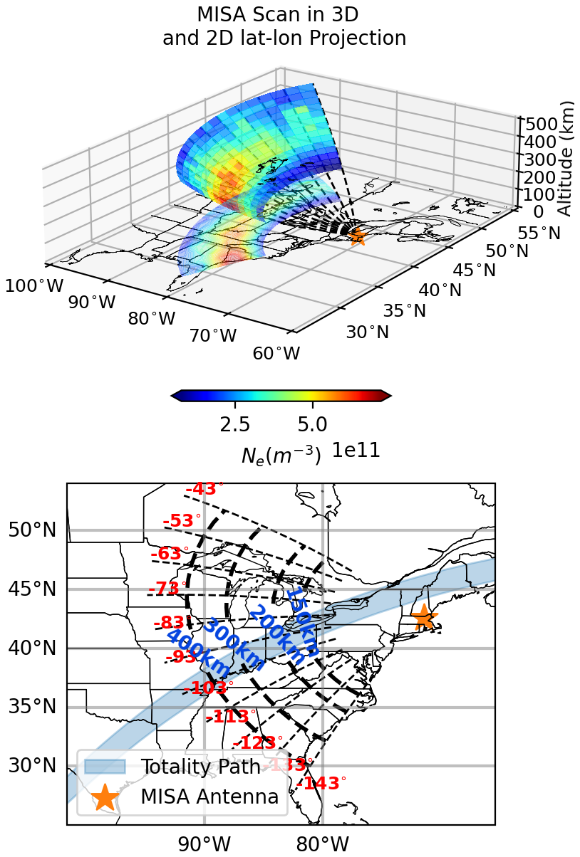
Figure 1 Upper panel shows N_e measurements from a 6° elevation MISA scanning experiment on the day of the eclipse. The latitude-longitude projection is displayed on the 0 km altitude plane. The second panel illustrates the approximate azimuth angles and altitudes of the MISA steerable antenna main beam across different scans on 8 April 2024 on a 2D plane. Totality path is superimposed on the diagram.

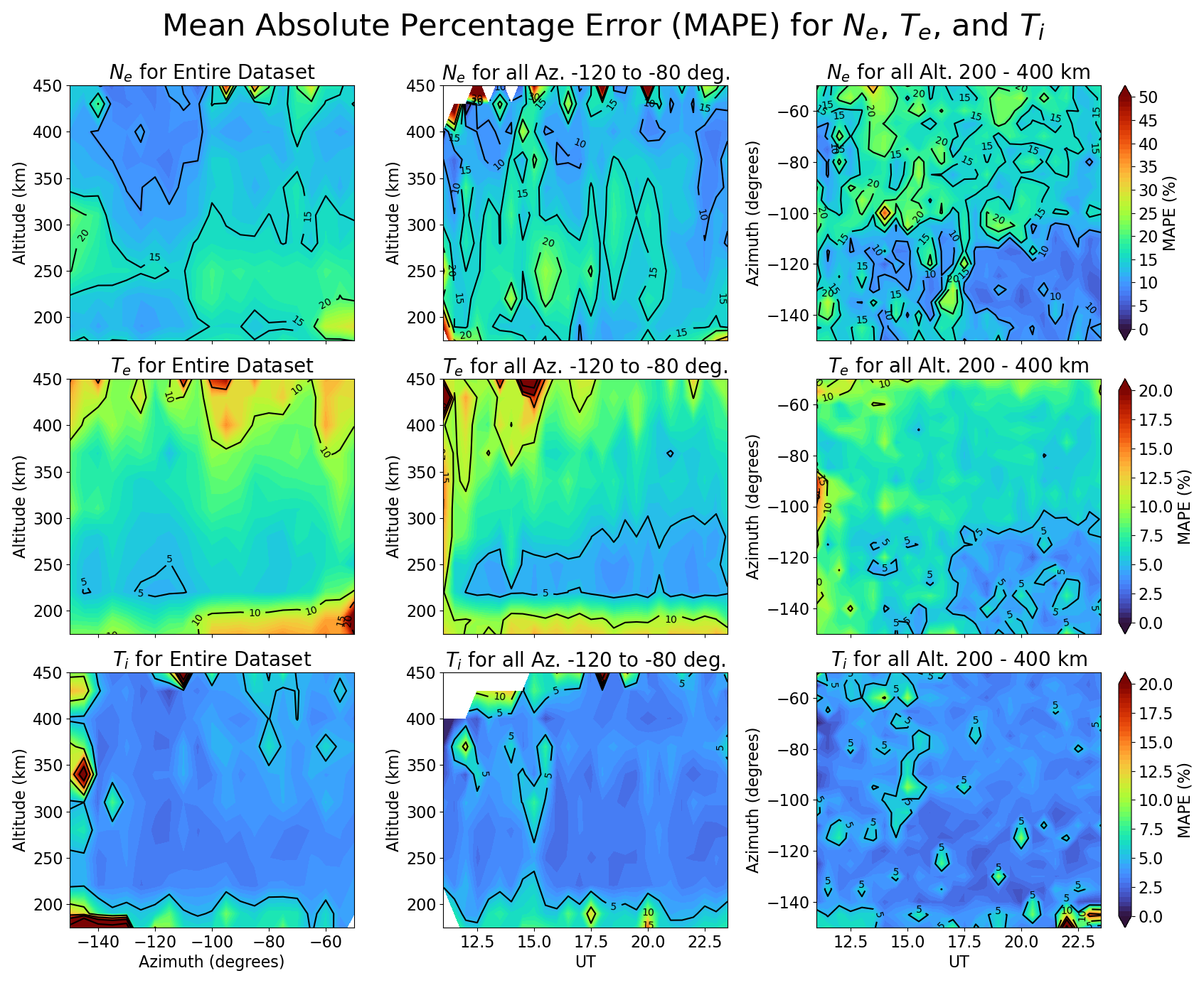
Figure 2 Mean Absolute Percentage Error (MAPE) for N_e, T_e and T_i for each 30 km altitude × 5° azimuth bin calculated using the entire training dataset (left column), for every 30 km altitude × 30 min UT bins averaged over azimuths between −120 to −80 (middle column), and for every 5° azimuth × 30 min UT bins averaged over 200–400 km altitude interval. MAPE values are in general less than 10 % for T_e, less than 5 % for T_i, and mostly less than 15 % for N_e with some regions less than 20 %.

Figure 2 illustrates the performance of the model and shows the Mean Absolute Percentage Error (MAPE) for N_e, T_e and T_i calculated using model predictions and corresponding MISA measurements. The first column shows the MAPE for azimuth and altitude bins for all days used in the training. For altitudes from 200–400 km, and azimuths above −140°, the MAPE is generally 15 % or less for N_e, 10 % or less for T_e, and 5 % or less for T_i. The second column shows the MAPE for azimuths between −120 to −80° which surround the path of the totality, and times from 12:00–23:00 UT. For altitudes from 200–400 km, and from 12.5 UT onward, the MAPE is generally 15 % or less for N_e, 10 % or less for T_e, and 5 % or less for T_i with MAPE values strongly decreasing after 15:00 UT.

The third column shows the MAPE binned according to azimuth and times from 12:00–23:00 UT for all altitudes between 200–400 km. For azimuths above −140°, and times later than 12.5 UT, the MAPE is generally 15 %–20 % or less for N_e, 10 % or less for T_e, and 5 % or less for T_i. According to the analysis above, and the criteria in Montaño et al. (2013), the model developed in this study can be considered in the good forecasting range for N_e, and in a highly accurate forecasting range for T_e and T_i.

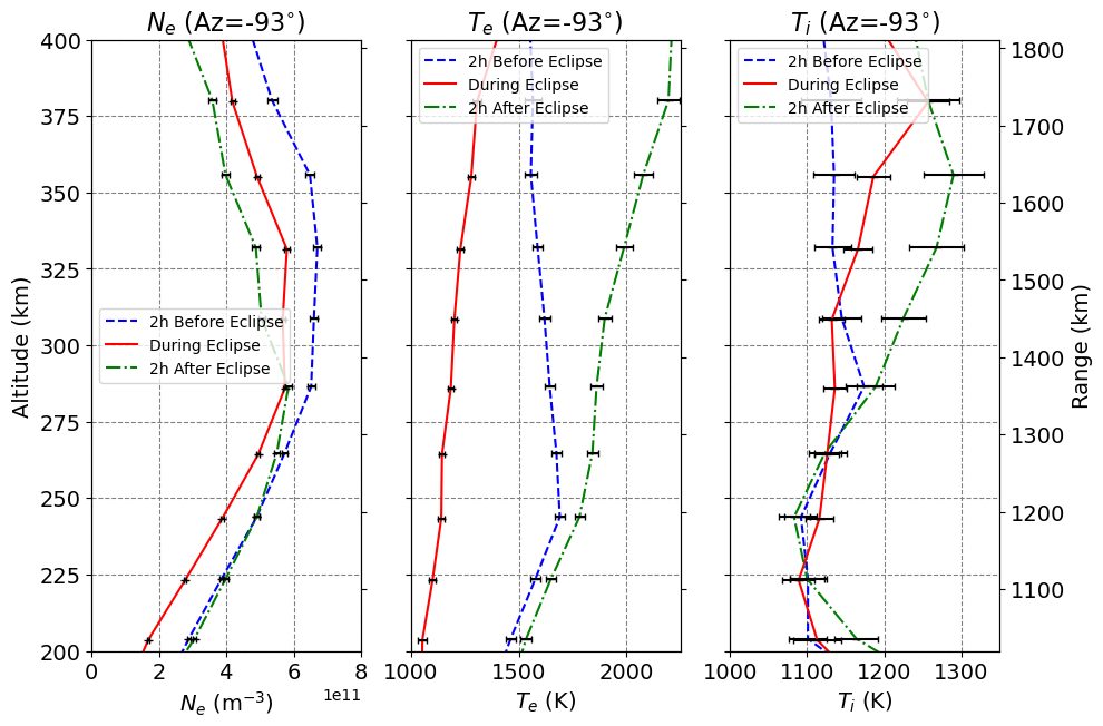
Figure 3 Altitude profiles of the observed N_e (left), T_e (middle) and T_i (right) 2 h prior to the eclipse (blue), during the eclipse (red) and 2 h after the eclipse (green).

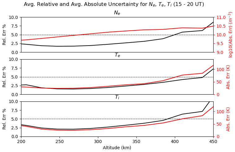
Figure 4 Altitude profiles of relative (in black) and absolute errors (in red) of N_e, T_e and T_i averaged over 15:00–20:00 UT and across all azimuths.

3 Results

Figure 5 shows latitude – longitude projections of N_e, T_e, and T_i observations from MISA scans on 8 April 2024. From left to right, each column corresponds to consecutive scans that occur before, during and after the time the totality passes over the MISA scanning region. Every panel represents 15 min of total experimental time with all of the 21 consecutive azimuthal scans (45 s duration) of a given experiment plotted simultaneously. Every parameter responds differently to the passage of the totality.

During the first scan (17:47–17:59 UT), the totality is located far southwestward from the scanning region, and parameter values correspond to measurements when obscuration percentages are less than 10 %. However, during the second scan (18:16–18:46 UT), the partial obscuration varies from 10 %–50 % substantially impacting EUV input, photo-ionization, and photochemical processes. During the third scan (18:46–18:58 UT), the totality moves from approximately 95° W and 34° N (shown by the red circle), to approximately 90° W and 37° N (shown by the grey circle) along the light grey path shown. In this timeframe, the totality overlaps with the outer edge of the scanning area corresponding to topside altitudes greater than 400 km, while obscuration percentages over the scanning region range from 90 % nearest to the totality to 50 % furthest from the totality. During the fourth scan (19:16–19:27 UT), the totality is located northeastward of the scanning region and obscuration percentages range from 60 %–90 %.

Every parameter responds differently to the eclipse spatially and temporally. N_e visibly decreases starting from the third scan and dips further during the subsequent scan by 2–3 × 10¹¹ around the F-peak region. The densities in the southern portion of the scans, approximately south of 42–45° N, are 2–3 times larger than those at northern latitudes and this difference becomes even more pronounced during the passage of the eclipse. The electron temperature (T_e) begins to decrease as early as the second scan and continues dropping further in the third and fourth scans with larger drops seen at lower altitudes between 200–300 km altitude. Drops of approximately 500 K are seen around 250 km altitude along the totality path between the first and fourth scans. The ion temperature (T_i) visibly decreases by the third scan along a path that is parallel and slightly south of the totality path along with an increase in T_i values southward of the totality path. This narrow drop in ion temperature is still visible in the fourth scan.

Figure 6 shows the evolution of N_e, T_e, and T_i post-eclipse during the next three consecutive scans and the final scan of the day (23:51–23:53 UT). There is little noticeable evolution of N_e from one scan to the next, and the lowest densities are seen in the second and third scans of the figure (20:15–20:26, 20:44–20:56 UT) where there is no longer any eclipse induced obscuration, indicating a delayed eclipse response, persistence of low densities, and slow recovery to typical background values. Similar to Fig. 5, densities are higher at southern latitudes, but N_e values south of 42–45° N are less than twice those at the north. The electron temperature (T_e) steadily increases in the first three scans over a period of approximately 1 h 15 min from 19:45–20:56 UT following the exit of the totality from the scanning region. The largest increases are seen in the topside. The increase is related to the low electron density values that persist following the eclipse. From 23:41–23:53 UT, we see a drop in T_e to typical nighttime values below 400 km altitude but high values persist at higher altitudes and larger azimuths for latitudes north of 40° N. Low ion temperatures persist along the same narrow path as in the previous figure during the first scan shown (19:45–19:57), but T_i changes become difficult to differentiate from background noise in subsequent scans.

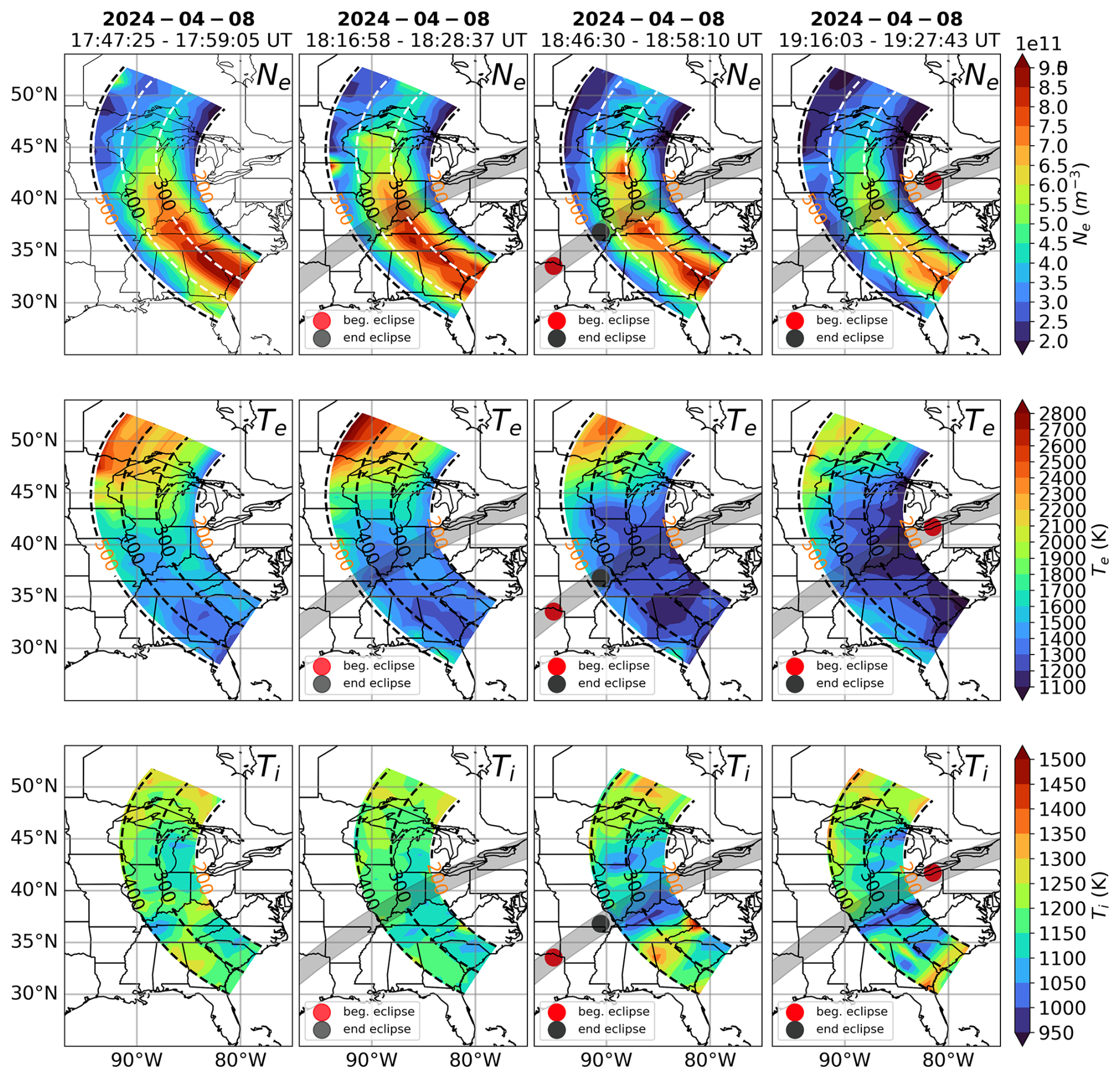
Figure 5 Azimuthal scans of N_e (top row), T_e (middle row), and T_i (bottom row) parameters on the day of the eclipse (8 April 2024) at four different times: prior to the eclipse passing over the scanning area, when the totality path overlaps with the furthest processed ranges of the scanning area (> 500 km altitude), when the totality path overlaps the nearest ranges of the scanning area (< 150 km altitude), and when the totality has moved eastward away from the scanning area. Red circles show the position of the totality during the first azimuthal scan and black circles show the position of the totality during the last azimuthal scan. Mild drop in N_e (second column) can be seen around 300 km when the totality approaches the furthest scanning area and continues to decrease much more in the next hour shown. The drop in T_e occurs at most latitudes and longitudes of the scanning region before the totality appears overhead, whereas N_e drops are visible when the totality is overhead. White or black dashed circular contour lines indicate the scanning altitude. Grey semi-transparent thick line indicates the path of the totality.

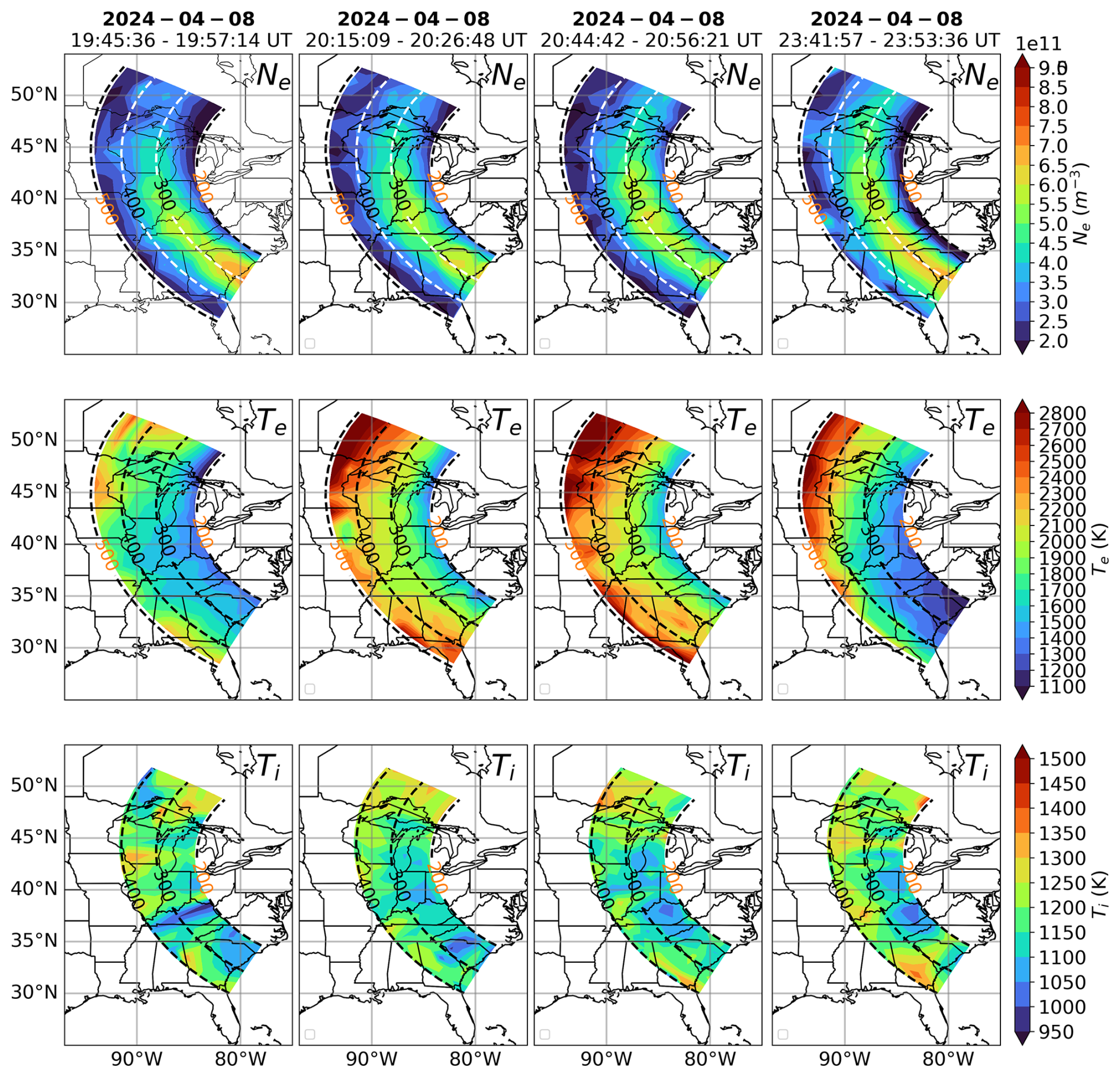
Figure 6 Same as Fig. 5 but for four subsequent scans. The first three columns display consecutive scans that occur immediately after those in Fig. 5, and the fourth column shows the scan which occurs at the end of the day (23:41–23:53 UT) to evaluate whether or not the parameters have recovered to pre-elipse levels.

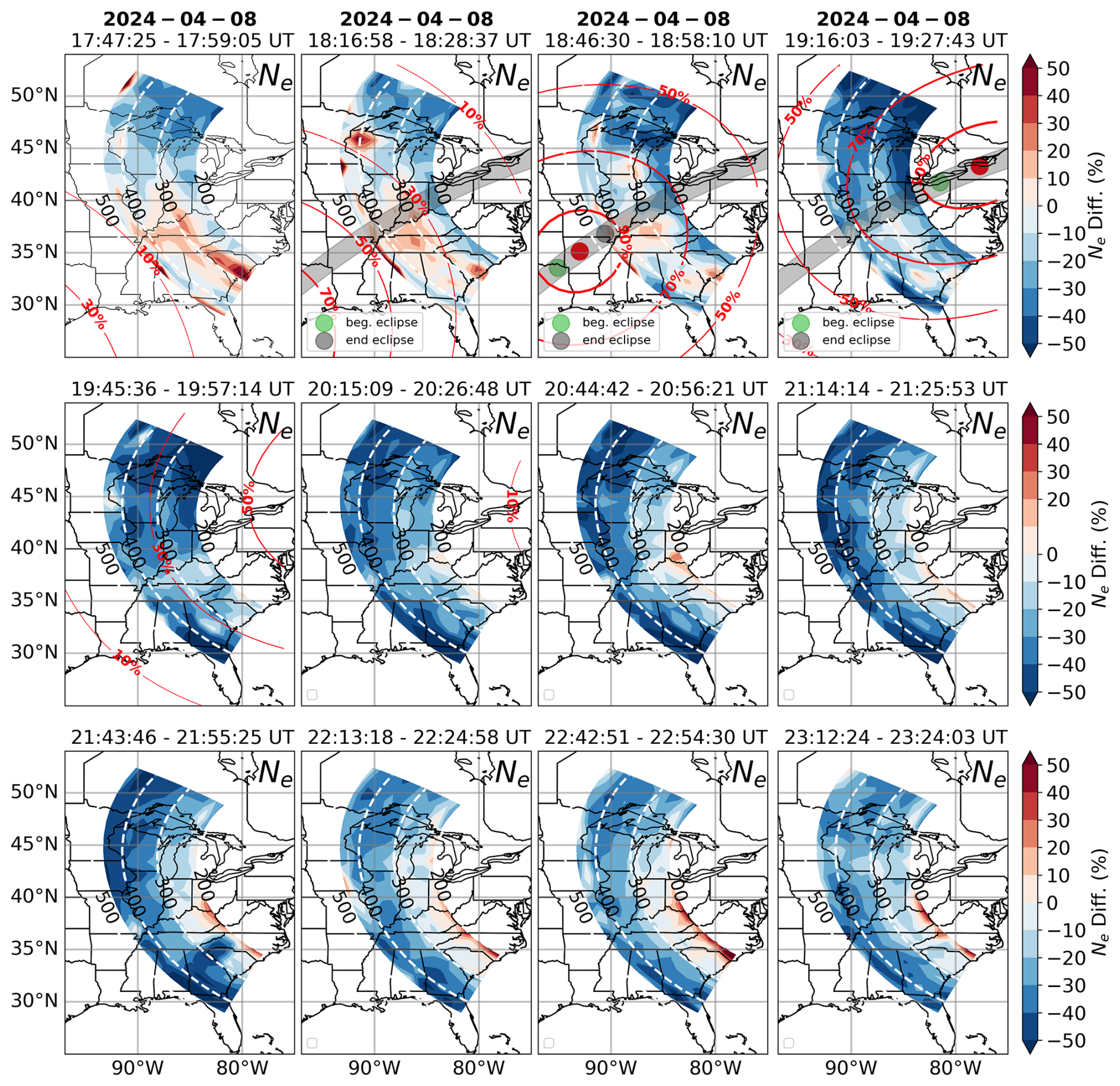
Figure 7 Percent difference MISA scan figures that show a difference between N_e observations and model predictions on 8 April 2024 for 12 consecutive MISA low elevation scans that cover the period before, during, and after the eclipse. Altitude contour lines and position of totality are shown as in previous figures along with eclipse obscuration percentage (red contour lines). N_e decreases are visible for the first time in the third scan and continue further in the fourth and fifth scans. Subsequent scans show F1 region recovery of N_e and topside persistence of decreased N_e values. Largest drops (40 %–50 %) of N_e appear at various latitudes and altitudes after the passage fo the eclipse.

Figures 7, 9, and 11 illustrate the percentage differences while Figs. 8, 10, and 12 show absolute differences between observed N_e, T_e, and T_i parameters and their model predictions on 8 April 2024. We show 12 consecutive scans prior to, during, and following the passage of the totality over the MISA scanning area with corresponding obscuration percentages superimposed over the scanning region and ranging from 0 %–100 %. In contrast to Figs. 5 and 6, indicating the percent and absolute parameter differences with corresponding background model predictions reveals features that are difficult to discern in the data scans.

In Figs. 7 and 8, N_e values begin to decrease more strongly north of the totality path and at low altitudes (third scan) and continue to decrease further at all altitudes and more uniformly across all latitudes although there is still a latitudinal asymmetry. The decrease in electron density of 40 %–50 % (2.0–2.5 × 10¹¹ m⁻³) is visible in the F1 region. Significant decrease in N_e then begins to spread to lower latitudes and is uniform across all altitudes (fifth scan). From the sixth to ninth scan, we can clearly see a recovery in N_e values that first take place in the F1 region (below 300 km) while the topside densities remain persistently low with values of 30 %–50 % (2.0–3.0 × 10¹¹ m⁻³) below predicted background levels. In the last three scans, N_e values appear to have recovered fully in the F1 region with partial recovery in the topside and N_e values 20 %–30 % (1.0–1.5 × 10¹¹ m⁻³) below background levels.

Figures 9 and 10 illustrate the electron temperature T_e response to the eclipse. T_e has a much faster response rate to variations in solar radiation caused by the eclipse and the drop in electron temperature appears proportional to the obscuration rate. The decrease in T_e occurs most strongly at latitudes (35–45° N) where the obscuration rates are larger. T_e begins to decrease visibly (10 %–20 % or 400–500 K) as early as the second scan over altitudes and latitudes where the obscuration rate falls between 30 %–50 %. By the third and fourth scans, there is a significantly larger decrease in T_e (30 %–40 % or 600–700 K) that spreads to a wider range of adjacent latitudes which occurs when obscuration rates above 70 % spread to a larger latitude interval. In fact, the geometry of these drops closely follows the obscuration geometry during the time of the scan. By the fifth scan, when the obscuration rates fall below 40 % in all scanning regions, T_e appears to have recovered to pre-eclipse levels. Following this, the next four scans show large increases in T_e anywhere from 10 %–40 % above background levels due to the persistence of low N_e values throughout the scanning region during the same timeframe. The largest increases of 10 %–40 % (700–800 K) occur between 30–35° N which also correspond to the same regions where large decreases in N_e are seen. In the last three scans, T_e values begin to decrease again to normal background levels and are less than 10 % higher than the background in the final scan.

Unlike N_e and T_e, the drop in T_i (Figs. 11 and 12) occurs over a much smaller range of latitudes along a latitude-longitude path parallel and slightly southward of totality path. During the third scan, a decrease of about 15 %–20 % (200–250 K) in T_i is visible along this path from 200–400 km altitude, with larger decrease seen from 250–350 km than below 250 km. At the same time, there is a mild enhancement in T_i of about 10 %–15 % parallel to the depletion but further south. The obscuration rate in the depletion region as well as the enhancement area is above 70 %. During the fourth scan, the totality has already crossed and exited the scanning region, and the obscuration rate overlapping the T_i depletion is still high (70 %–90 %) but narrower and spread more uniformly over all altitudes shown. In addition, it appears as though the mild enhancement in T_i has now moved to the southernmost azimuths and another depletion has appeared in its place. In the subsequent scan shown in the fifth time interval, a weakened depletion is still visible with mild enhancements at all latitudes north of the depletion. However, in all subsequent scans, depletions and enhancements are less than 10 % (100 K) of the predicted background values, and it is difficult to assess whether they are eclipse related or simply connected to the model and data variance. It is interesting to note however, that in the ninth and tenth scans (21:14–21:25, 22:13–22:24 UT) there are enhancements of 100–200 K in the same region as the eclipse related depletions in earlier scans.

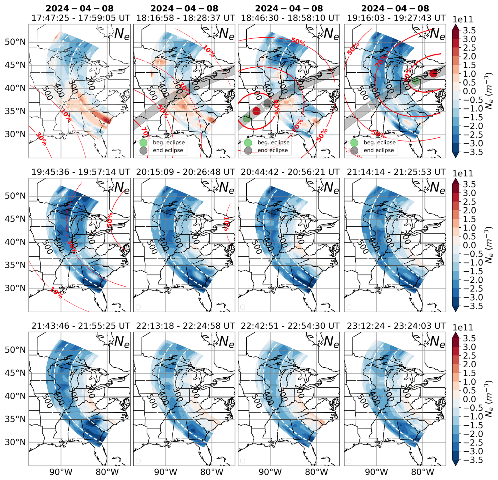
Figure 8 Similar to Fig. 7 but for absolute values of N_e data-model differences.

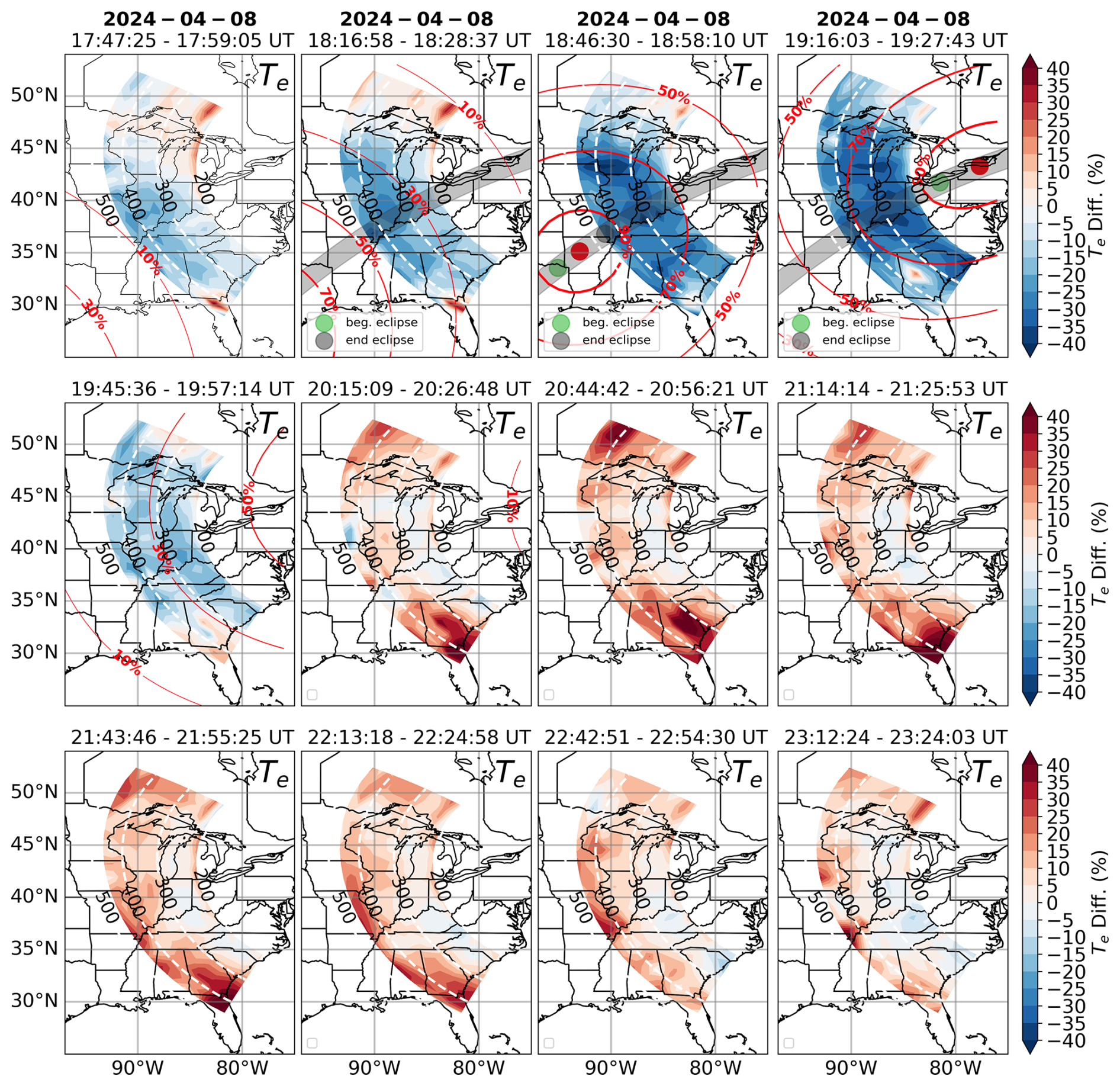
Figure 9 Percent difference MISA scan figures that show a difference between T_e observations and model predictions on 8 April 2024 for 12 consecutive low elevation scans for the period before, during, and after the eclipse. Altitude contour lines and position of totality are shown as in previous figures along with eclipse obscuration percentage (red contour lines). T_e decreases are visible for the first time in the second scan and continue further in the third and fourth scans. Subsequent scans show recovery of T_e and increase to higher than background values at all altitudes immediately after the obscuration is no longer present. The largest drops in T_e of 40 %–50 % appear at all altitudes at the latitudes that surround the path of the totality or where the obscuration is highest.

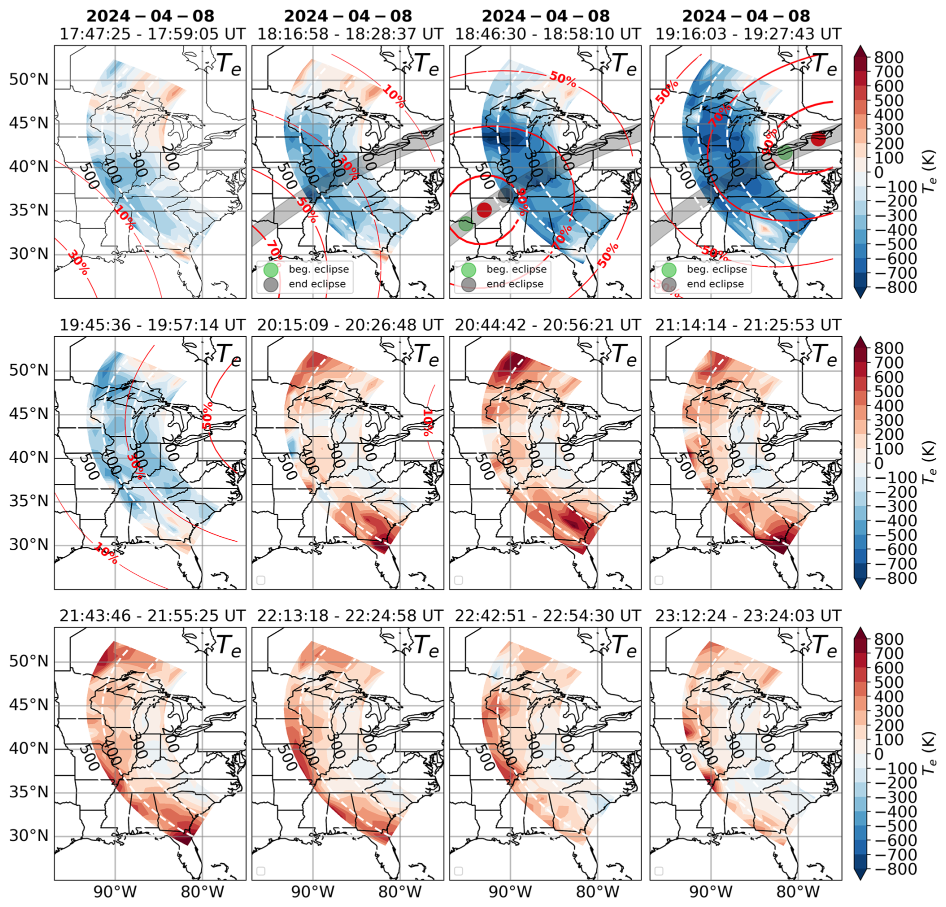
Figure 10 Similar to Fig. 9 but for absolute values of T_e data-model differences.

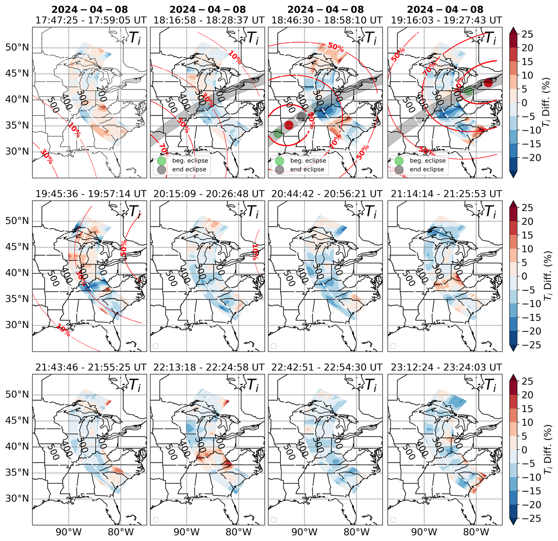
Figure 11 Percent difference MISA scan figures that show T_i model predictions on 8 April 2024 subtracted from T_i data measurements covering 12 consecutive low elevation scans for the period before, during, and after the eclipse. Altitude contour lines and position of totality are shown as in previous figures along with eclipse obscuration percentage (red contour lines). T_i decrease is visible for the first time in the second scan in a region parallel and slightly south of the path of the totality. The largest decrease (15 %–20 %) appears in the third scan and becomes less pronounced in the fourth and fifth panel. Subsequent scans where the obscuration is no longer present show recovery of T_i to background levels.

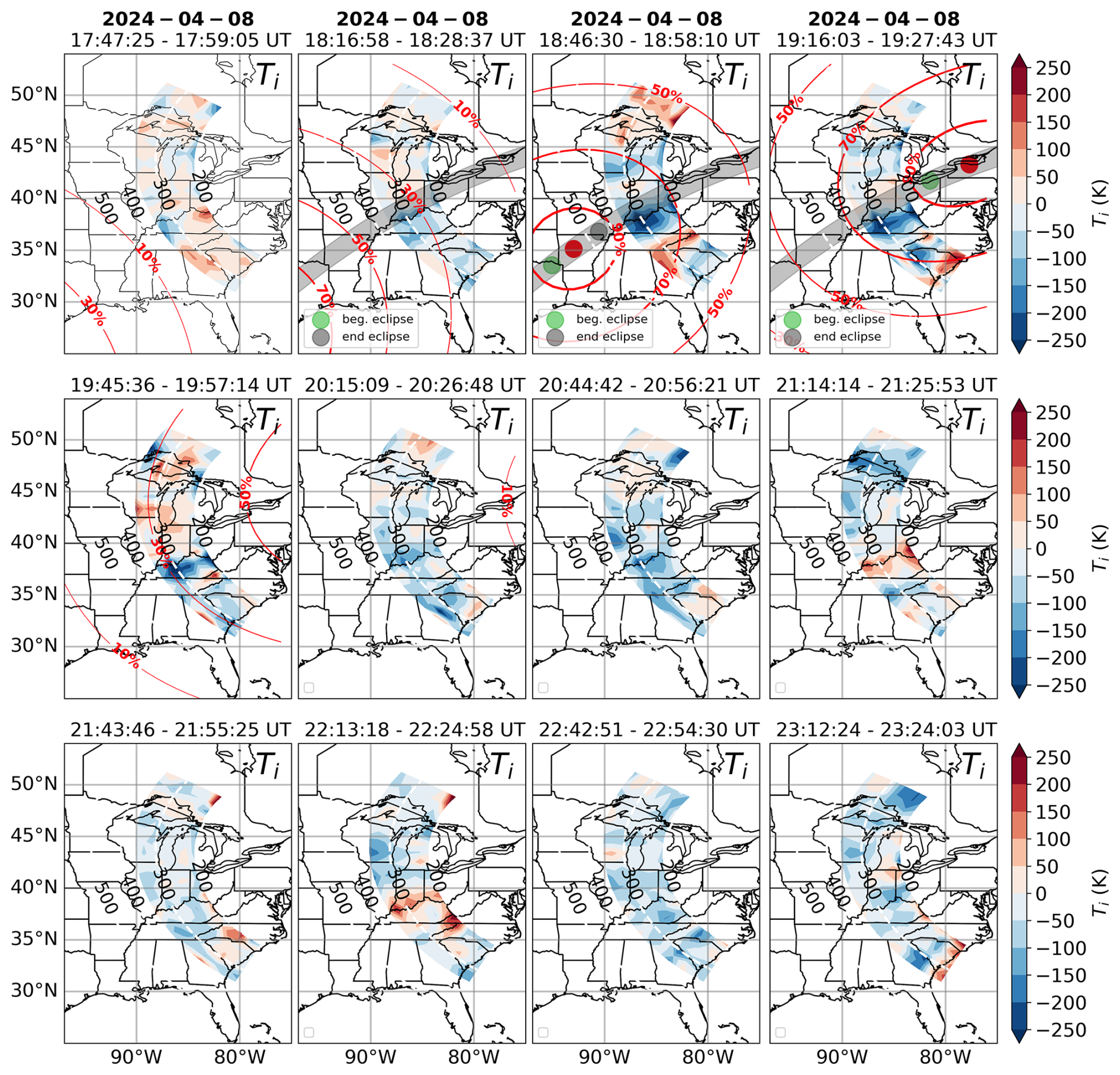
Figure 12 Similar to Fig. 11 but with absolute decrease values of T_i.

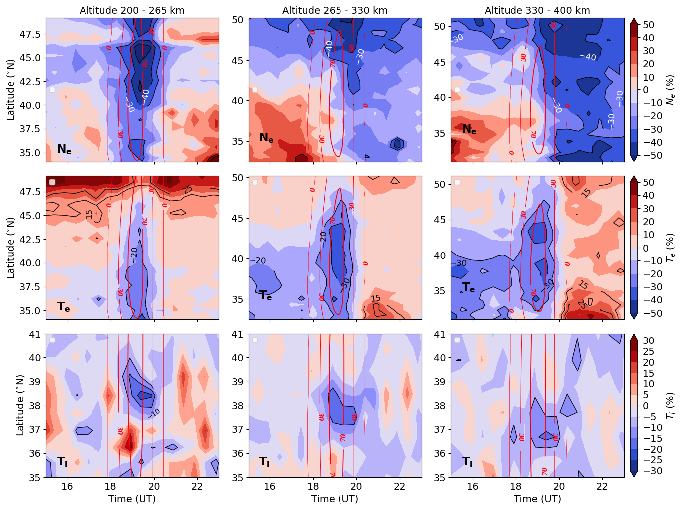
Figure 13 Each column of this figure displays the percent difference between data and model for N_e, T_e, T_i at a given latitude over the time interval of 15:00–24:00 UT and for parameters averaged over three equal altitude sub-intervals from 200–400 km: 200–265 km (left column), 265–330 km (middle column), and 330–400 km (right column). Eclipse obscuration percentage is shown using red contour lines. The largest drops in N_e from 40 %–50 % occur above 40° N. T_e decreases are seen from 18:00–20:00 UT and do not persist later in the day as for N_e. T_i decreases from 10 %–15 % along a narrow range of latitudes which correspond closely to the path of the totality.

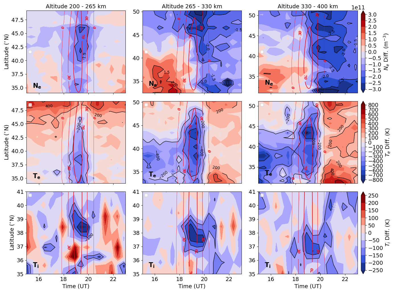
Figure 14 Same as Fig. 13 but showing changes in absolute parameters (N_e, T_e, and T_i). The largest overall decrease in densities ranging from 2.5–3 × 10¹¹ m⁻³ is seen from 265–300 km altitude and above 40° N within 1 h of the closest approach time of the totality. Strong decrease of equivalent value is seen in the topside and south of 35° N. T_e shows the largest drops of 400 K from 40–45° N above 265 k altitude. Increases of 250 K are seen after 20:00 UT most strongly in all azimuths from 400–450 km altitude. T_i shows a decrease of about 200–250 K in a small range of latitudes parallel to the path of the totality and lasts from the red dashed line to approximately 21:00 UT.

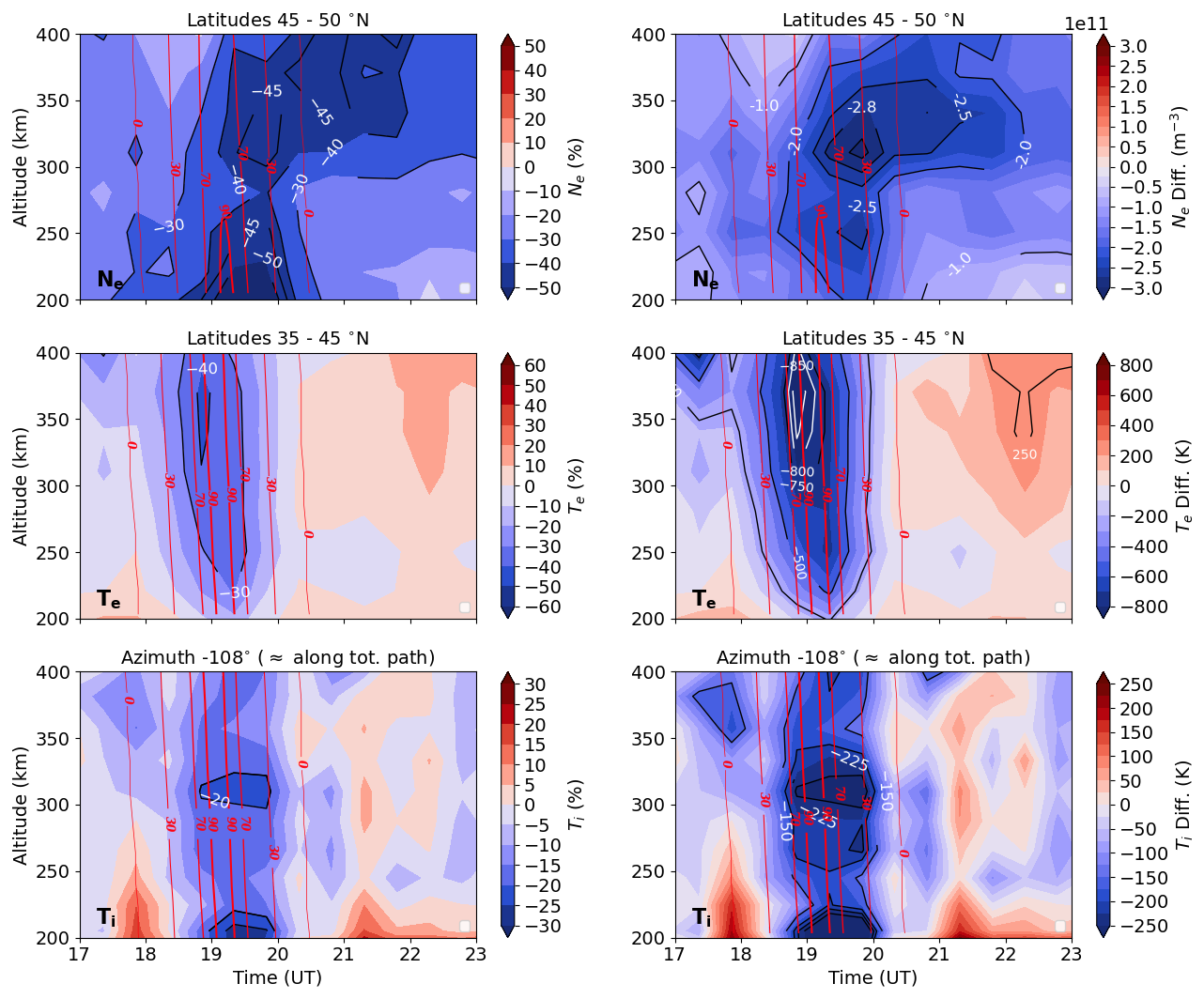
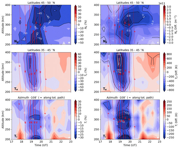
Figure 15 Percent (left column) and absolute right column) difference between data and model for N_e, T_e, T_i at all altitudes from 15:00–24:00 UT averaged over latitudes from 45 to 50° (N_e), 35 to 45° (T_e), and along a single scanning azimuth of −108° which corresponds closely to the path that is parallel and slightly southward of the path of the totality. This figure captures the altitudinal behavior of the parameters over time. Eclipse obscuration percentage is shown with red contour lines. F1 region N_e, T_e, and T_i show immediate recovery when obscuration is no longer present, whereas topside N_e persists until 22:00 UT.

Figures 13 and 14 show percent and absolute difference between data and model for altitude averaged N_e, T_e, and T_i parameters at given latitudes (∼ 34–55° N) vs time (15:00–24:00 UT). Every column corresponds to parameters averaged over three sub-intervals between 200–400 km: 200–265 km (left column), 265–330 km (middle column), and 330–400 km (right column). The largest percentage drops in N_e occur at northern latitudes (mostly north 40–45° N) and persist longer at higher altitudes. For the lowest altitude range from 200–265 km, the largest decrease in N_e ranges from 45 %–50 % (2.8–3×10¹¹ m⁻³) below the predicted background values and occurs between 40 to 50° N, lasting for from 19:00–20:00 UT and corresponding to the time when the highest obscuration is present. In the second altitude interval from 265–330 km, the largest decrease in N_e from 45 %–50 % (2.8–3×10¹¹ m⁻³) occurs above 47° N and also lasts approximately from 19:00–20:00 UT. However, there is a milder decrease that lasts until 22:00 UT. In the third altitude interval of 330–400 km, the largest decrease in N_e from 45 %–50 % (2.8–3×10¹¹ m⁻³), occurs above 47° N as well as below 33° N and lasts from 19:00–22:00 UT with milder decreases persisting until 23:00 UT. In addition, N_e values within the lowest altitude interval appear to respond proportionally to the obscuration rate and begin to decrease immediately after the obscuration rate climbs above 0 % at 18:00 UT. For the intermediate altitude range, N_e begins to decrease much later on around 19:00 UT for latitudes below 43° N but slightly earlier at 18.5 UT when the obscuration rate reaches 30 %. Non-eclipse related decrease of N_e is visible at much earlier times and overlaps with eclipse induced decreases. This could be due to the model prediction variance. At the highest altitude range spanning 330–400 km, N_e first begins to decrease from the eclipse around 19:00 UT.

In contrast to the electron density, the electron temperature decreases appear to extend from 35–45° N or approximately the latitudinal location of the totality path and extend approximately equally in the north and south direction from this path. The shape of the depletion area in latitude and time corresponds very closely to that of the obscuration percentage contour lines. Unlike the electron density, the decrease in T_e is more limited in latitude. There is a very mild decrease in electron temperature (T_e) attributable to the eclipse north of 45° N and south of 35° N. The largest absolute drop in T_e of 600–800 K occurs around 44° N and 19:00 UT in the topside (330–400 km in altitude) and occurs simultaneously with an obscuration percentage of 100 %.

In addition, T_e begins to decrease as early as the obscuration rate rises above 30 % at the lowest altitude interval for most latitudes but appears to respond immediately when the obscuration rate increases beyond 0 % for latitudes between 37.5 and 40° N. Even though it is highly likely that this also occurs for the higher altitude intervals, temperature decreases due to geomagnetically or TID induced elevated N_e from 15:00–19:00 UT and from 33–40° N overlap with eclipse induced decreases and make the latter harder to distinguish. Similarly, slightly before 20 UT, electron temperatures start to resume to normal background values when the obscuration falls below 30 %, and then continue to increase to higher than background values. Subsequently, increases in T_e (< 200 K or less than 10 % in the F1 region and 200–400 K or between 10 %–30 % in the topside) occur because of lower electron densities that persist at all altitudes but especially in the topside.

Like the electron temperature, ion temperatures (T_i) also begin to decrease as soon as the obscuration rate exceeds 30 % but persist slightly longer until about 21:00 UT. Unlike electron temperature drops, ion temperature decreases are restricted to one or two latitude-longitude paths parallel to the path of the totality, and they do not increase above background values post-recovery for the two upper altitude intervals. However, there are regions of increased T_i from 36–37° N from 18.5–19:00 UT, and from 21:00–23:00 UT and between 36–40° N. The largest decrease in T_i from 15 %–20 % (150–200 K) is located between 37–39° N and during the maximum obscuration rate.

Figure 15 illustrates the percent and absolute difference between data and model for N_e, T_e, T_i from 15:00–24:00 UT for all altitudes averaged over latitude windows that showed the strongest decreases in Figs. 13 and 14. The purpose of the figure is to capture the altitudinal variation in the temporal response of the parameters to the eclipse. In the upper row, N_e is averaged over latitudes from 45 to 50° N. The decrease in N_e values shows an altitude dependent response and recovery time with the lowest altitudes responding immediately as soon as the obscuration percentage increases beyond 0 %, and fully recovering before the obscuration reaches 0 % again. N_e also shows the strongest percent decrease (from 45 %–50 %) at the lowest altitudes 200–250 km. However, the strongest absolute decrease is a drop in N_e of 2.8–3.0 × 10¹¹ m⁻³ from 300–350 km altitude which is due to the large densities in the F-peak region. In the topside region from 300–400 km, N_e remains 40 % lower than background levels up to 22:00 UT, and 30 % lower until the 23:00 UT thus never fully recovering. The largest drop in T_e (40 %–50 % or 850–900 K) occurs above 350 km altitude. Like in the previous Figs. 14 and 13, eclipse associated drops in T_e respond almost immediately to the change in obscuration percentage. Lower altitudes show weaker decrease. The biggest drops in T_i (25 %–30 % and 225–250 K) occur in two distinct regions: one from 300–325 km altitude, and another from 200–225 km for which the percent drop in N_e is also large. Unlike for T_e, the largest drop in T_i occurs where the electron density is the largest, namely in the F-peak region, and also where the percent drop in N_e is the largest and the drop in T_e is weakest, namely at the lowest altitudes.

4 Discussion

This is the first study to our knowledge that leverages the unique capabilities of a steerable wide-field incoherent scatter radar to investigate the impact of near total obscuration on ionospheric parameters such as N_e, T_e, and T_i over a large geographic region of the continental US. In contrast to previous reports of ISR-based observations which have focused on vertical variations of these state parameters, in this study we extend our understanding into the horizontal domain. Most of the scanning region was subjected to obscuration percentages larger than 75 % at eclipse time. Some results presented in Figs. 8–15 show latitudinal and altitudinal features that are in agreement with previous observational and modeling studies. Other results represent novel features unique to this study, such as induced ion temperature cooling that reached 225 K, among the largest ion temperature drops reported during an eclipse. Other novel observations are cooling that occurred within a narrow region parallel to the totality path, and asymmetric N_e decrease between the north and south of the totality path.

4.1 Electron density response to the eclipse

The eclipse-induced ionospheric response in N_e is complex and depends on a large number of parallel mechanisms and factors. These effects combine to produce reduced photoionization rates, low temperature and pressure induced downward plasma diffusion, modified diffusion rates, and eclipse induced low pressure systems that can modify thermospheric winds and thus plasma transport (Aa et al., 2024; Ding et al., 2010; Le et al., 2009).

The observed electron density response time to the solar eclipse increased with altitude despite higher altitudes being subjected to the eclipse obscuration earlier. This is consistent with the expected ionospheric photochemical and diffusive processes which responded to the sudden reduction in photoionization. This increasing eclipse response time with altitude as seen in Figs. 7, 8, 13, 14 was consistent with TIDAS 3-D ionosphere data assimilation results (Aa et al., 2024). The authors in (Aa et al., 2024) attribute this slower response time to the balancing effect of downward plasma diffusion caused by a change in the plasma equilibrium scale height from a decrease in plasma temperature and pressure at lower altitudes. This behavior was also demonstrated in the TIEGCM simulation for the August 2017 solar eclipse over Millstone Hill (Wang et al., 2019). The effect is furthermore seen in other modeling and observational studies (Goncharenko et al., 2018).

The N_e recovery time was also altitude dependent but with very large differences between the topside and the F1 region. In the F1 region, the recovery time was nearly uniform up to the F-peak and roughly corresponds to the return of pre-eclipse photoionization levels, whereas in the topside it occurred 3–4 h later. Faster photoionization processes in the F1 region drove the newly generated plasma upward along magnetic field lines toward the topside, but this process was slow and takes significant time. Additionally, the recovery timing below the F-peak in the afternoon (after 20:00 UT ∼ 15:00 LT ) with larger solar zenith (weaker photoionization) and enhanced plasma temperature (smaller downward flux) prevented prompt recovery of the topside ionospheric and even plasmaspheric density (Aa et al., 2024; Wang et al., 2019) through diffusion, even though the diffusion velocity grows rapidly as a function of height.

Thermospheric winds are also significantly perturbed during an eclipse, and form an additional dynamic factor. Numerous modeling studies point to the effect of thermospheric disturbance winds that can cause low pressure systems and create a wind convergence point towards the eclipse region (Choudhary et al., 2011; Cnossen et al., 2019; Wang et al., 2019; Müller-Wodarg et al., 1998; St.-Maurice et al., 2011; Yan et al., 2021) The increased wind induced ion-neutral collisions drag plasma along field lines from lower to higher altitudes, or vice-versa (depending on the direction of the winds), and can substantially modify the existing photochemically triggered changes in N_e.

In this study, a latitudinal asymmetry in eclipse induced density depletions was clearly seen in the scanning region (Fig. 7) 1–2 h after the passage of the totality. For example, in the third, fourth and fifth scans of Fig. 7, latitudes north of the totality path experienced a greater percent decrease in N_e values than the latitudes below. Simulations of thermospheric wind convergence point dynamics from the 2017 solar eclipse indicate its location trails totality by approximately 1 h (Cnossen et al., 2019; Wang et al., 2019)

Applying this factor to the 2024 eclipse, as the wind convergence point approached the scanning region (fourth scan) from the southwest, it generated large southwestward disturbance winds. Because the declination angle over the scan area varies from −10 to 0°, the plasma was pushed along the field lines mainly by the meridional wind component. This led to the plasma being lifted upwards along the field lines by these eclipse-induced disturbance winds, which blow against the regular daytime poleward winds. Although perhaps minor, this effect could have opposed to some degree any eclipse driven N_e decrease in the topside (visible as higher densities in the topside between 40–45° N close to the totality path as compared to above 45° N). The topside region south of the totality path also experienced weakened eclipse induced decrease except for the southernmost portion of the scanning region where the disturbance winds were weaker and eclipse induced lower densities remain unopposed. During the fifth scan, which occurs 1 hour after the third scan, we can approximately assume that the wind convergence point was located very near or even overlapped the southwestern portion of the scanning region, causing the winds south of the totality path to be oriented northward. Northward oriented winds would then reduce the density in the topside by driving plasma down the field lines. This is consistent with observations of a continued decrease in N_e south of the totality path, which caused the overall latitudinal asymmetry in the scanning region to become less pronounced. From the sixth to the eighth scans, daytime poleward thermospheric winds returned to pre-eclipse background levels, and the latitudinal N_e depletion asymmetry in the topside region became negligible leading to uniform decrease at all latitudes.

Another plausible factor for electron density dynamic response could be related to geomagnetic storm ionospheric response. From 15:00–18:00 UT, substantially elevated electron densities of up to 50 % from typical background values were observed south of 40° N, with strongest N_e increase in the F-peak region (265–330 km altitude in Figs. 13 and 14). This N_e increase could have been potentially related to elevated geomagnetic activity and should not be confused with eclipse related effects. A brief increase in geomagnetic activity occurred between 06:00–09:00 UT, with Kp >3, leading to a delayed ionospheric response at mid latitudes ∼ 6–8 h later. This range of time delay in ionospheric parameters at Millstone Hill in response to geomagnetic activity was also noted earlier in (Zhang and Holt, 2008).

Since the regression model is unable to accurately predict effects of specific geomagnetic activity, the influence of earlier increases in the Kp index could show up as elevated densities in data-model differences. However, these effects are not likely a major driver in this particular eclipse, and further modeling study would be required to gauge the relative importance of this mechanism.

4.2 Electron temperature response to the eclipse

The ionospheric electron temperature exhibited significant changes during this eclipse. A T_e drop up to > 800 K was much larger than 100–200 K observed in the 2017 (partial) eclipse at Millstone Hill, and was similar to 500–700 K seen in the 30 May 1984 solar eclipse (Salah et al., 1986) and 800–1000 K in the 20 July 1963 solar eclipse (Evans, 1965). Electron energy transfers to the ambient ions through Coulomb collisions at a rate that is proportional to squared electron/ion density in the F region. Thus a strong anti-correlation between N_e and T_e in the F region is very evident and has been previously well documented (Zhang et al., 2004; Zhang and Holt, 2004). The ion temperature itself depends additionally on neutral temperature and therefore T_i also provides feedback to T_e. As a result, there exists thermal balance among T_e, T_i and T_n at night as well as at lower altitudes, but T_e > T_i > T_n during the day in the F region. Furthermore, electron thermal conduction across altitudes may become an important factor in the topside when the bottomside T_e drops (Huba and Drob, 2017; Zhang et al., 2021b; MacPherson et al., 2000).

Our 2024 observations suggest that the eclipse effect on T_e likely involved (1) reduced solar irradiation as the main energy source for photoionization (photoelectrons) and photoabsorption (T_n), (2) the influence of subsequently reduced N_e on T_e enhancement, and (3) thermal conduction in the higher F region as a result of large T_e height gradients during different solar eclipse stages. It appears that effects (1) and (3) were dominant during the eclipse onset and recovery periods; effect (2), and perhaps effect (3), became more evident during post-eclipse periods when the solar irradiation became stable but N_e was still gradually recovering.

4.3 Ion temperature response to the eclipse

Observations presented in this study offer a unique opportunity to evaluate the spatio-temporal response of ion temperature to a solar eclipse, including the magnitude, temporal development, and geographic extent of the response. Similarly to changes in T_e, variations in T_i are among the least understood ionospheric perturbations, due to the shortage of both observations and simulations that focus on plasma temperature responses. In addition, eclipse induced variations in ion temperature are smaller than those in electron temperature and are thus harder to separate from typical short-term variations that could arise, for example, from traveling ionospheric disturbances (Panasenko et al., 2018).

Still, there is a significant body of evidence that T_i during eclipses decreases by ∼ 50–150 K. Domnin et al. (2013) reported a T_i drop of up to 140 K during the 1 August 2008 eclipse (solar minimum) with obscuration of 42 %. Grigorenko et al. (2008) and Cherniak and Lysenko (2013) found a 30–70 K decrease in T_i for a 29 March 2006 solar eclipse with an obscuration of 73 %, also for solar minimum conditions. Salah et al. (1986) indicated relatively little variation in T_i in response to the solar eclipse on 30 May 1984 with an obscuration of 86 %, although the electron temperature T_e decreased dramatically, by up to 700 K at 300–500 km altitude. A potential ∼ 120 K T_i response was observed around ∼ 190 km, but it diminished by ∼ 300 km. Similarly, Pitout et al. (2013) could not discern T_i variations in response to the solar eclipse of 1 August 2008 in the EISCAT ISR data, although T_e decrease exceeded 1200 K. Goncharenko et al. (2018)'s study of the 21 August 2017 solar eclipse revealed a T_i cooling by up to 140 K for conditions with a maximum obscuration of 63 %, with maximum cooling observed at 150–230 km altitude, and ∼ 70 K cooling seen at 250–300 km altitudes.

In our study, the ion temperature cooling observed during 8 April 2024, reached 225 K, among the largest ion temperature drops reported during an eclipse. This large decrease in ion temperature is likely related to the fact that it occurs in the area close to the maximum obscuration rate. The altitudinal variation of the decrease in T_i shows two clear peaks at ∼ 260–325 km and at ∼ 200 km, but lower cooling at altitudes above ∼ 350 km. We note that this is consistent with earlier results from vertical-only studies that reported noticeable T_i cooling in a limited range of altitudes (Salah et al., 1986; Grigorenko et al., 2008; Goncharenko et al., 2018) and weaker T_i decrease at higher altitudes. This behavior contrasts with GITM simulations that predict stronger T_i cooling at higher altitudes, specifically ∼ 200 K cooling at 400 km in comparison with 50–75 K cooling at 200 km (Cnossen et al., 2019). Simulations with SUPIM-INPE of the 14 December 2020, eclipse showed an altitudinal pattern of T_i changes similar to the GITM simulations, with T_i cooling exceeding 50 K at altitudes above ∼ 550 km, but much lower perturbation in T_i below ∼ 450 km (Bravo et al., 2022). There is no clear explanation for the disparity between simulations and observations in the altitudinal variations in ion temperature changes due to the eclipse, and further modeling study is required beyond the scope of this article. This discrepancy also points to needed improvements in energetics for full profile modeling attempts to understand ionospheric thermodynamics and its connections to ionosphere-thermosphere coupling. These future modeling improvements, such as more realistic upper boundary conditions or more correct light neutral and ion species (H, He, H+, He+), could resolve the discrepancy.

The temporal variation of the eclipse-induced T_i decrease for the most part was consistent with expectations from simulations (Wu et al., 2018; Cnossen et al., 2019), with T_i response symmetric with regards to the maximum obscuration time, as expected due to the decrease in EUV heating. The largest T_i decrease occurred shortly after the largest obscuration (Figs. 13, 14, 15), indicating close coupling between the ion and electrons. However, post-eclipse recovery did not reveal a clear increase in T_i in the area of a large increase in T_e, in contrast to simulations (Cnossen et al., 2019; Bravo et al., 2022). Additionally, according to simulations, the geographic area of a significant T_i decrease is expected to extend to at least 20° in latitude and longitude (Cnossen et al., 2019). Observations in 2024 showed a more complex behavior, with areas of both negative and positive T_i disturbances within the radar’s field of view. This behavior could result from quasi-periodic disturbances in multiple ionospheric parameters with 20–120 min periods that were seen during this (Aa et al., 2024) and other eclipses (Burmaka and Chernogor, 2013; Kumar et al., 2013; Panasenko et al., 2019), associated with AGW generated at lower altitudes. A superposition of a general T_i reduction driven by the decrease in solar EUV and quasi-periodic perturbations due to AGW could have created a complex response seen in Figs. 11 and 12.

4.4 Space Debris Considerations

From our present analyses of MISA ISR data, the main difficulty presented by “hard target” space debris comes from in-beam reflections due to the Starlink operational belt at 550 km altitude. The much larger cross-section of the satellite bodies themselves, combined with any debris in the orbit plane, yields a heavily distorted signal and prevents any incoherent scatter measurements. However, Millstone Hill observations show that this does not prove an operational problem for realistic ionospheric parameter profiles at altitudes significantly away from the Starlink orbital shell, and with the steerable MISA antenna at off-vertical directions (6° elevation) as is used in our study. These conclusions are based on comparisons during non-eclipse conditions to empirical based models of ionospheric parameters (Zhang and Holt, 2008) and to the standard IRI model. In particular, the wide field results from the steerable MISA antenna do not show any hard target distortions to beyond the sensitivity range of even the longest radar pulse used. Detailed calculations of the relative cross-section of ionospheric Thomson scatter versus satellite debris are beyond the scope of this paper, and are not even possible at present as the flux of 34 cm debris is not sufficiently characterized in orbit.

5 Conclusions

In this study, we presented regional ionospheric parameter changes associated with the 8 April 2024 solar eclipse in the eastern to central United States, using 6° elevation wide sweep azimuth scans from the Magnetosphere-Ionosphere Steerable Antenna (MISA) of the Millstone Hill Incoherent Scatter Radar. To the best of our knowledge, this is the first report that presents simultaneous observations of the altitude-resolved response of N_e, T_e, and T_i to a solar eclipse over a broad geographic area, as prior studies were limited to observations in a single direction. In contrast to other studies that used limited multi-day averages to characterize pre-eclipse background ionospheric conditions, we used a polynomial regression model to predict the background ionosphere, and subtracted model-predicted values from the observed values to determine absolute and percent variations of electron density, electron temperature, and ion temperature due to the influence of the eclipse. Significant spatial and temporal differences were found in each parameter's response to the eclipse.

The response of N_e to the eclipse strongly depended on latitude. Significantly larger percent and absolute drops occurred at the northernmost latitudes (north of 45° N) within 1 h of the appearance of the totality over the scanning region. Drops of up to 50 % and 3 × 10¹¹ m⁻³ were recorded at these latitudes. This latitudinal asymmetry in electron density drops is due to the influence of disturbed thermospheric winds which trail the totality and move plasma up or down the magnetic field lines differently south and north of the totality path. Approximately 1.5 h after the totality first overlaps the western edge of the scanning region, the much weaker poleward neutral background winds dominated once again, and the drop in N_e values spreads uniformly to all latitudes.

The response of N_e to the eclipse passage and post-eclipse recovery was also strongly altitude dependent. N_e responded earlier, and showed a faster recovery rate in the F1 region in comparison to the topside due to differences in photochemical and diffusive processes which reacted to a sudden reduction in photoionization. For altitudes ranging from 200–265 km, a decrease in N_e values was seen as early as 18:00 UT when the obscuration rate was just above 0 %, with a recovery to normal background levels slightly after 20:00 UT (obscuration rate nearing 0 %). In comparison, there was an increasing delay in the response time of N_e for altitudes above 350 km. Above 350 km altitude, N_e responded after 19:00 UT (after the obscuration reached a minimum of 70 %) and began to recover significantly only after 22:00 UT, without a full recovery even by the end of the day. The slower recovery rates in the topside were due to weaker photoionization rates in the F1 region during the onset of the eclipse, the dominance of slower diffusion processes, and enhanced plasma temperature preventing prompt recovery of the topside through diffusion.

The largest drops in T_e during the eclipse onset occurred at latitudes closest to the totality path where the obscuration is largest, because the dominant T_e decrease mechanism is reduction in photoionization. The T_e response time showed a relatively flat altitude profile from 300–400 km in contrast to N_e, and temperature decrease began when the obscuration varied from 0 %–30 % between 18:00 and 18.5 UT. This indicates that reduced photoelectron production in the F1 region led to: (1) local F1 region cooling and (2) topside cooling due to simultaneous decrease of photoelectron flux into the topside where the dominant heating mechanism is non-local transport. We showed that drops of up to 40 % (850 K) occur for altitudes above 325 km averaged between 35–45° N from 18.75–19.25 UT. Increases of 200 K and 10 %–15 % in temperature were visible after 20.25 UT due to the lower electron densities which persisted at higher altitudes post-eclipse. In general, observations indicate that the eclipse effect on T_e involved multiple factors including reduced photoionization rates in the F1 region, the effect of reduced N_e on T_e enhancement, and possibly thermal conduction in the higher F region as a result of large T_e height gradients.

Eclipse triggered decreases in ion temperature (T_i) occurred when the obscuration percentage reached 30 %, and T_i recovered to normal levels after the obscuration rate decreased below 30 %, shortly after 20:00 UT. The strongest decreases of 20 % or 225 K occurred from 19:00–20:00 UT at two distinct altitude regions below 225 km and between 300–325 km altitude within a narrow geographic region parallel to the path of the totality. The temporal, altitudinal and latitudinal response of T_i, which included a T_i drop along a narrow region and T_i enhancements that shifted latitudinally from one scan to the next, suggest the possible superimposition of quasi-periodic perturbations due to AGW to a general eclipse-induced T_i decrease.

In aggregate, the observations discussed in this study provide unique evidence of closely tied ionospheric and thermospheric processes and present a new challenge to current models of coupled ionosphere and thermosphere. Although numerous simulations have separately evaluated the roles of direct reduction in solar EUV, changes in the neutral temperature and wind system, and changes in thermospheric composition during solar eclipses, the simultaneous and coupled contributions of changes in electron density and electron and ion temperature, and their impact on energy exchange between electrons, ions, and neutrals, remain poorly understood. Further examination of these processes will also provide new insights about ion-neutral coupling mechanisms under dynamically changing solar irradiation conditions.