Parameterization of the subsolar standoff distance of Earth's magnetopause based on results from machine learning

The subsolar standoff distance r₀ of Earth's magnetopause is a key parameter in understanding the interaction between the solar wind and the magnetosphere. Despite decades of modeling efforts, significant uncertainties persist between model predictions and satellite observation of the magnetopause location. This study introduces a new data-driven parameterization of r₀, based on a dataset containing over 220,000 dayside magnetopause crossings obtained by the THEMIS (2007–2022) and Cluster (2001–2020) missions. Each crossing is paired with high-resolution upstream solar wind parameters from the OMNI database. Four established empirical models are benchmarked against this dataset, yielding root-mean-square errors (RMSE) of ≳1 R_E globally and ≳0.8 R_E in the subsolar region. To determine the primary physical factors of r₀, an XGBoost regression model is trained and interpreted using SHapley Additive exPlanation (SHAP) values. The solar wind dynamic pressure is found to be the dominant contributor, followed by geomagnetic indices (AE, SYMH), interplanetary magnetic field (IMF) magnitude, dipole tilt angle, and IMF cone angle. The IMF B_z component contributes only marginally when geomagnetic indices are included. A support vector regression (SVR) model using the six most influential parameters achieves a RMSE of 0.68 R_E, improving on the best analytic model by approximately 17 %. A second-order polynomial expression with 14 terms is derived, providing a compact, interpretable, and accurate representation of r₀. The SVR model and the polynomial representation is not able to predict r₀ for extreme input conditions, e.g., during the passage of interplanetary coronal mass ejections. Accordingly, the parameter ranges that define the validity domain of the models are specified. The presented results offer improved predictive accuracy of the subsolar standoff distance and highlight the role of so far unconsidered parameters in modeling Earth's magnetopause.

1 Introduction

Earth's magnetopause is the boundary layer between the interplanetary magnetic field (IMF) and the terrestrial magnetic field. It therewith separates solar wind plasma from Earth's magnetosphere and controls its size. To first order, the magnetopause forms at pressure equilibrium of the solar wind dynamic pressure p_dyn and the magnetic pressure exerted by Earth's magnetic field. Since the dynamic pressure is the main factor controlling the location of the magnetopause, early models to describe its shape and location depend on this parameter (e.g. Fairfield, 1971). Additionally, the IMF B_z component is identified as an important parameter and incorporated in following models (e.g. Roelof and Sibeck, 1993; Shue et al., 1997). That is because the direction and magnitude of the B_z component drives dayside magnetic reconnection, where field lines of Earth's magnetic field connect to the IMF, particularly when it is southward (e.g. Petrinec et al., 2022, and references therein). As a result, the magnetopause moves closer to Earth because of dayside flux erosion (Aubry et al., 1970).

The functional form of the model by Shue et al. (1997) characterizes the magnetopause via the subsolar standoff distance r₀, that is the distance between Earth's center and the magnetopause on the aberrated (see below) Sun-Earth line, and the flaring α; a parameter determining how open the magnetopause is on the nightside:

$$\begin{array}{}\text{(1)}& r_{\mathrm{mod}}=r_{\mathrm{0}}\cdot {\left({\displaystyle \frac{\mathrm{2}}{\mathrm{1}+\cos \left(\mathit{\theta }\right)}}\right)}^{\mathit{\alpha }},\end{array}$$

where θ is the solar zenith angle (referred to as zenith angle in the following). Shue et al. (1998) find

$$\begin{array}{}\text{(2)}& r_{\mathrm{0}}=(\mathrm{10.22}+\mathrm{1.29}\cdot \tanh (\mathrm{0.184}\cdot (B_z+\mathrm{8.14})\left)\right)\cdot p_{\mathrm{dyn}}^{-\frac{\mathrm{1}}{\mathrm{6.6}}}\end{array}$$

and

$$\begin{array}{}\text{(3)}& \mathit{\alpha }=(\mathrm{0.58}-\mathrm{0.007}\cdot B_z)\cdot (\mathrm{1}+\mathrm{0.024}\cdot \ln (p_{\mathrm{dyn}}\left)\right)\end{array}$$

empirically, based on mostly equatorial magnetopause crossings (MPCs) by different satellites orbiting Earth. The model is referred to as Sh98 hereinafter. The Sh98 model is axis symmetric around the aberrated Sun–Earth line and does not include cusp indentations. Despite, or perhaps because of, its simplicity, the Sh98 model is regularly used to this day (see e.g. Wang and Sun, 2022; Cucho-Padin et al., 2024). Still, there is an ongoing effort to develop new models that better reflect the actual shape and position of the magnetopause. A visible trend is the increased model complexity in both the amount of parameters used and structure of the parameterization. Newer models account for, e.g., the dawn-dusk asymmetry (Walsh et al., 2014; Baraka et al., 2021; Janda et al., 2024), and include terms for cusp indentations.

One example is a magnetopause model by Lin et al. (2010), called Lin10 in the hereforth. The magnetic pressure p_mag is added as an input parameter, accounting for the pressure of the IMF on the magnetopause. Additionally, the tilt angle γ of Earth's dipole in the (y,z) plane is an input parameter. Because the azimuth angle is also used to parameterize the magnetopause, the model is not axis symmetric anymore. The empirical model is based on 2708 MPCs of different satellites. In total, the model contains 21 coefficients, underscoring the complexity due to the additional input parameters. Based on the MPC dataset used to construct the model, the Lin10 model outperforms previous magnetopause models, including Sh98, in terms of prediction accuracy.

Liu et al. (2015) utilizes the same parameters as in Lin10 with the addition of the IMF B_x and B_y components. Therewith, the IMF is included fully and not only by B_z. Liu et al. (2015) use a magnetohydrodynamics (MHD) approach to find dependencies between r₀ and the input parameters to construct their model (named Liu15 in the following). The influence of the B_y component is discussed in Aghabozorgi Nafchi et al. (2023) with the conclusion that it influences the radial distance of the magnetopause.

In contrast, Nguyen et al. (2022c) use the clock angle and the IMF B_z component separately to cover the influence of the IMF on the shape of the magnetopause in their model (referred to as Ng22 hereinafter). The clock angle represents the projected direction of the IMF in the (y,z) plane and is computed via ${\mathit{\theta }}_{\mathrm{clock}}=\arctan \mathrm{2}(B_y,B_z)$, with a range from −180 to 180°. A value of $\left|{\mathit{\theta }}_{\mathrm{clock}}\right|>\mathrm{90}\mathit{°}$ therefore means southward IMF configuration. While Aghabozorgi Nafchi et al. (2023) find the clock angle to be important in magnetopause modeling, Case and Wild (2013) see no dependence of model performance and clock angle.

The four aforementioned models all use rather typical solar wind and IMF parameters and are either based on MHD simulations or empirical studies, using a best–fit approach to a given parameterization. However, magnetopause models could potentially be improved by considering other input parameters (Němeček et al., 2020b) or methods (Wang et al., 2013; Aghabozorgi Nafchi et al., 2024). In this study, we apply machine learning (ML) techniques to address both ideas. First, the parameters most suitable for the parameterization of the subsolar standoff distance of the magnetopause are identified. The influence of each parameter on r₀ is investigated in detail in the following, before a novel parameterization of the subsolar standoff distance is developed.

2 Data and Preprocessing

Empirical magnetopause models are typically based on datasets of MPCs by different spacecraft. This work uses two extensive MPC catalogs, one for the Time History of Events and Macroscale Interactions during Substorms (THEMIS) (Angelopoulos, 2008) and one for the Cluster mission (Escoubet et al., 2001). The THEMIS catalog (TH–MPC) (Grimmich et al., 2023a) contains a total of 184 292 dayside MPCs between 2007 and 2022. All five THEMIS satellites (THA–THE) are included in the catalog; however, THB and THC are only present until the end of 2009, as they transitioned to the ARTEMIS mission thereafter. Due to the orbital configuration of the THEMIS spacecraft, the TH-MPC catalog covers the low latitude regime up to about ±30° latitude, with full dayside longitude coverage. The MPCs are identified by a random forest machine learning classifier. Accordingly, each MPC is associated with a probability that quantifies the algorithm's confidence in its classification as an MPC. For more detail on the process, see Grimmich et al. (2023b). The Cluster catalog (CL–MPC) (Grimmich et al., 2024a) comprises of 38 322 individual MPCs by the C1 and C3 spacecraft between 2001 and 2020. The polar orbit of the Cluster satellites allows for a greater coverage of the high latitude dayside and cusp regions. Although CL–MPC includes considerably fewer MPCs than the TH-MPC catalog, it thereby remains highly valuable. Note that CL–MPC contains nightside crossings as well, with a split of roughly 60/40 dayside/nightside crossings. Grimmich et al. (2024b) utilizes a modified version of the random forest classifier applied for the TH–MPC catalog to determine magnetopause crossing locations. Combining both datasets, a maximum of 222 614 MPCs can be used for magnetopause modeling.

In addition to the crossing probability, each MPC entry includes the crossing time in UT and position in Geocentric Solar Ecliptic (GSE) coordinates, along with other associated parameters. In GSE, the x-axis points towards the Sun, the z-axis is normal to the ecliptic plane and the y-axis completes the right-handed coordinate system, pointing in antiparallel direction of Earth's orbital motion. In a spherical GSE representation, the zenith angle θ is defined as the angle between r and the positive x direction ($\mathit{\theta }=\arctan \mathrm{2}(\mathit{\rho },x)$, where ρ is the distance from the x-axis: $\mathit{\rho }=\sqrt{y^{\mathrm{2}}+z^{\mathrm{2}}}$, $\mathit{\theta }\in [\mathrm{0},\mathit{\pi }]$). The azimuth angle $\mathit{\phi }=\arctan \mathrm{2}(z,y)$ is the angle of the position vector projected onto the (y,z) plane measured from the positive y-axis towards the positive z-axis ($\mathit{\phi }\in [-\mathit{\pi },\mathit{\pi }]$).

A number of solar wind and IMF parameters for each crossing time are obtained from the OMNI database (Papitashvili and King, 2020). The OMNI database comprises mostly WIND and ACE satellite data, monitoring space weather at the L1 point on the Earth-Sun line. The data is timeshifted to the bowshock nose in order to specify the conditions at Earth at a given time (King and Papitashvili, 2005). Crucial parameters for this study are, e.g., the IMF components B_x, B_y, B_z, the solar wind velocity components v_x, v_y, v_z, the proton density, the alpha particle to proton ratio $\mathrm{Na}/\mathrm{Np}$ and the ion temperature. All coordinate dependent quantities are in the GSE system. Derived quantities such as the IMF (B) and solar wind velocity (v) magnitude, the proton dynamic pressure p_dyn, the magnetic pressure p_mag, and the alfvenic and magnetosonic Mach number are calculated for every MPC. As the clock and cone angles of the IMF are characteristic parameters to describe the IMF configuration, they are also determined for every MPC. The cone angle specifies the angle between the IMF vector and the B_x component and is calculated via ${\mathit{\theta }}_{\mathrm{cone}}=\arccos \left(\right|B_x|/B)$. It has a range of 0 to 90°. The typical Parker-spiral configuration of the IMF is represented by θ_cone≈45°, while smaller values indicate sunward or anti-sunward (radial) IMF and larger values correspond to a perpendicular IMF.

Additionally, the geomagnetic Auroral Electrojet (AE) and Symmetric Horizontal Magnetic Disturbance (SYMH) indices at the time of a MPC are matched to the corresponding MPC. The SYMH index (Imajo et al., 2022) is taken directly from the OMNI database. It essentially resembles a high resolution (1 min) version of the Dst index, which is used to study the activity of geomagnetic storms (Wanliss and Showalter, 2006; Menvielle et al., 2011). The AE index also has 1 min resolution and represents the magnitude of geomagnetic activity associated with the eastward and westward auroral electrojets. Thus, it is a measure for substorm activity, with increasing values meaning stronger substorm behavior (Menvielle et al., 2011). The OMNI database provides the provisional AE index up to 2019 (inclusive), and the quick look AE index from 2021 onward (Nose et al., 2015). The World Data Center (WDC) for Geomagnetism, Kyoto, further provides the provisional AE index for the first half of 2020. For the second half of 2020, no AE data is available for download at the time of this work.

The MPC times are aligned to the nearest minute to match the corresponding high-resolution 1 min OMNI data. The data is not timeshifted further to account for the time delay between the bowshock and the magnetopause. Because of occasional gaps in the OMNI database, about 25 % of all crossings are missing at least one of the aforementioned parameters. To mitigate this circumstance and enlarge the percentage of usable MPCs, a symmetric 10 min interval of OMNI data around the crossing is looked at. The mean value of the available data for each individual parameter is assigned to the corresponding parameter at the time of the MPC. MPCs gaining data via this process are flagged for later recognition. This approach allows 71 % of the MPCs with initially missing parameters to be utilized, increasing the data coverage significantly. Still, a fraction of MPCs remains, for which some parameters are not available. In cases where essential parameters for further analysis are missing, the associated MPC is omitted from the analysis.

Due to Earth's orbital velocity v_E, the magnetospheric system is not perfectly aligned with the GSE x-axis but is instead aberrated by a few degrees. The aberration angle ψ arises from the relative motion between the solar wind and Earth, and depends on both the solar wind speed v and Earth's orbital velocity v_E, which is assumed to be constant at 30 km s⁻¹. The aberration angle can be approximated by

$$\begin{array}{}\text{(4)}& \mathit{\psi }=\arctan \left(-{\displaystyle \frac{v_{\mathrm{E}}}{v}}\right),\end{array}$$

and is calculated individually for every MPC. The aberration angle typically lies between −2.7° and −5.6°. Equation (4) is a simplification of the exact formula $\mathit{\psi }=\arctan (v_{⟂}/v_x)$, where $v_{⟂}=v_y+v_{\mathrm{E}}$. Since the v_x component dominates the solar wind direction, v_x≈v can be assumed safely. The v_y component however is often not small compared to v_E, especially not in the fast solar wind where the flow deflection has a median value of 18 km s⁻¹ (Němeček et al., 2020a). Including the v_y component would increase the absolute aberration by almost two degrees which especially affects the position of the MPCs on the nightside. In the subsolar region, the aberration of the position is neglected since the effect is smaller and the absolute value of the magnetopause distance, which is unchanged by the aberration correction, is more important for our model than the exact position of the MPC. By rotating coordinate sensitive parameters, such as the position and the IMF, by ψ around the z-axis, the system is transformed into aberrated GSE (AGSE) coordinates. Again, the transformation is done for each MPC separately with its respective aberration angle. Derived quantities (like the clock and cone angles, the zenith angle, etc.) are then recomputed in AGSE format. A comparison of the AGSE IMF components derived with this method to those obtained when the aberration includes the v_y component (see above) shows discrepancies of only a few tenths of a nanotesla. We argue that the uncertainty in the IMF data is larger than this deviation and therefore use the simplified equation for the aberration. Including v_y could be considered in future studies to account for the aforementioned effects more precisely. MPCs where no solar wind data is available from OMNI cannot be converted to AGSE by Eq. (4). In such cases, the mean aberration angle (−4.16°) could be applied to enable the use of these crossings in further analysis. However, crossings with missing solar wind data frequently also lack IMF data, which makes them unusable regardless. Consequently, these crossings are excluded from the dataset. The combined dataset then contains 206 764 MPCs. For the modeling done in this work, the AGSE system is used.

Looking closer at the magnetopause crossings reveals that the random forest algorithm often classifies numerous MPCs by the same spacecraft in short succession. This is not per se atypical since the magnetopause is in motion and may cross the satellite multiple times in a short period of time. However, it is likely that the algorithm made false positive detections of a MPC despite extensive validation effort. Grimmich et al. (2023b) points out that an additional source for successive MPCs is a Low Latitude Boundary Layer next to the magnetopause which makes a precise classification more difficult. To filter possible misidentified MPCs, crossings with a probability of less than 0.75 are excluded from further analysis. As a result, the remaining combined database comprises 146 478 MPCs (∼66 % of all MPCs). In the next sections, the maximum number of MPCs is further limited by the zenith angle and the parameter availability for each crossing.

3 Magnetopause Model Performance Comparison

In an attempt to better predict the position and shape of the magnetopause, recent models have become increasingly more complex, accounting, e.g., for the cusp indentation, the dawn–dusk asymmetry, Earth's dipole tilt angle, and effects of the IMF on the magnetopause position. Hence, it is expected that the shape and location of the magnetopause will vary between different models, even under identical input conditions. Cross-sections of the Sh98, Lin10, Liu15, and Ng22 magnetopause models are displayed in Fig. 1. The (a) terminator, (b) y=0, (c) and equatorial plane is shown separately. The IMF is in southward Parker Spiral configuration while the solar wind dynamic pressure is the mean of the whole dataset (2.1 nPa). The dipole tilt angle is set to 25° to better identify differences of the models. Notably, the subsolar standoff distance appears to be rather similar for all models. Also, the equatorial dayside magnetopause only shows small deviations in all models. At the terminator, the difference between the Sh98/Lin10 and Ng22 model already exceeds 2 R_E in the southern hemisphere, further increasing on the far nightside. While the Sh98 model is circular in the (y,z) plane, all others are not due to the cusp indentations (see especially Lin10) and a rotation induced by the IMF (mostly notable for Liu15). Liu15 and Ng22 are very similar and symmetric in the equatorial plane. For the far night side, they predict a smaller dawn-dusk extension than the other two models. The Lin10 model shows a strong dawn-dusk asymmetry. In the y=0 plane, the Sh98 model exhibits multiple R_E deviations in the cusp regions with respect to the other three models. It also stands out that the dipole tilt has an influence on the nightside magnetopause, rotating it further north (south) in the northern (southern) hemisphere for positive (negative) angles for all but the Sh98 model, where it is not included. In conclusion, the different magnetopause models largely agree on the subsolar standoff distance and the low latitude dayside regime, while the magnetopause position at the high latitude dayside and cusp regions and the nightside vary significantly. For more extensive comparisons of magnetopause models on different datasets, see, e.g., Case and Wild (2013), Suvorova and Dmitriev (2015), Samsonov et al. (2016), Němeček et al. (2020b), Nguyen et al. (2022b), and Lin et al. (2024). In the following, the prediction capability of each model is investigated for the dataset introduced in Sect. 2.

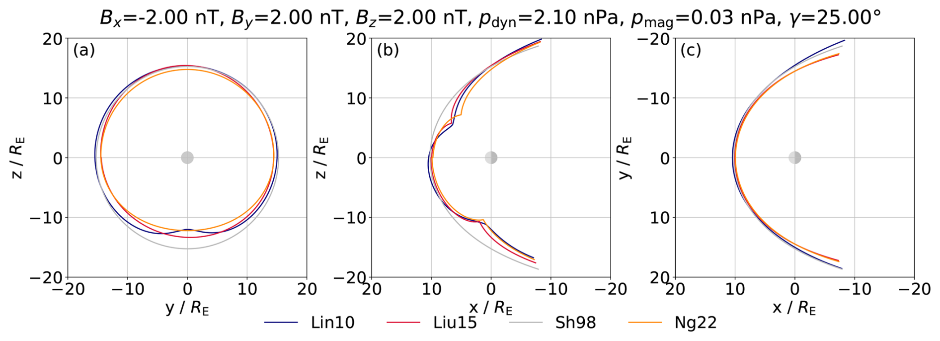
Figure 1 Magnetopause shapes of the Sh98, Lin10, Liu15, and Ng22 models in (a) the terminator, (b) the y=0, and (c) equatorial plane in AGSE coordinates. Note that for panels (b) and (c) the x-axis is flipped, so that the Sun is located on the left.

3.1 Dayside Magnetopause

The dayside region is characterized by x>0 (θ<90°). Because the CL–MPC dataset contains nightside crossings, the amount of usable MPCs reduces to 137 295 after they are filtered out. Since all mentioned magnetopause models rely on the IMF B_z component, MPCs with missing IMF data cannot be used for model comparison. This leaves 133 045 usable MPCs. For each crossing, the magnetopause distance r_mod is calculated for the four models with their respective formula. The observed magnetopause distance by the spacecraft is the magnitude of the positional vector of the magnetopause crossing and denoted as r_obs. To determine the accuracy of each model, the prediction error

$$\begin{array}{}\text{(5)}& \mathrm{\Delta }r=r_{\mathrm{obs}}-r_{\mathrm{mod}}\end{array}$$

is calculated for each crossing. Histograms of the resulting Δr distributions are shown in Fig. 2. Notably, the four models perform rather equally with a common root-mean-square error (RMSE) of slightly above 1 R_E. The mean values of the Sh98 and Lin10 model are close to zero, indicating good magnetopause prediction capabilities on average. For Liu15, the positive mean error implies a small underestimation of the model, meaning that the magnetopause is more expanded than the model assumes for given input parameters. Similarly, the Ng22 model underpredicts the real magnetopause extend by almost 0.5 R_E. The standard deviation of of the prediction error is about 1 R_E for all models, mostly contributing to the RMSE. Figure 3 shows Δr over the zenith angle in a heatmap for the four models. The red dots with error bars indicate the mean and standard deviation of the prediction error for a 4.5° wide bin. The heatmap reveals larger deviations from zero and an increased error for larger zenith angles for every model, especially for θ>60°. These findings imply that the models exhibit reduced predictive accuracy in regions approaching the terminator and possibly on the nightside, consistently estimating the magnetopause to be at larger distances to Earth than it actually is, on average. As discussed for Fig. 1, the models deviate the most in the nightside low latitude regime, suggesting that the shape of the nightside magnetopause is not fully understood (partly due to little available data) or fluctuates largely despite similar conditions. Regardless of the differences of the models in that region, none of the models is able to make accurate predictions. For lower zenith angles (θ<60°), the models on average slightly underpredict the magnetopause distance, especially the Ng22 model, resulting in the high mean Δr value. The Lin10 model seems to be the most accurate for smaller zenith angles.

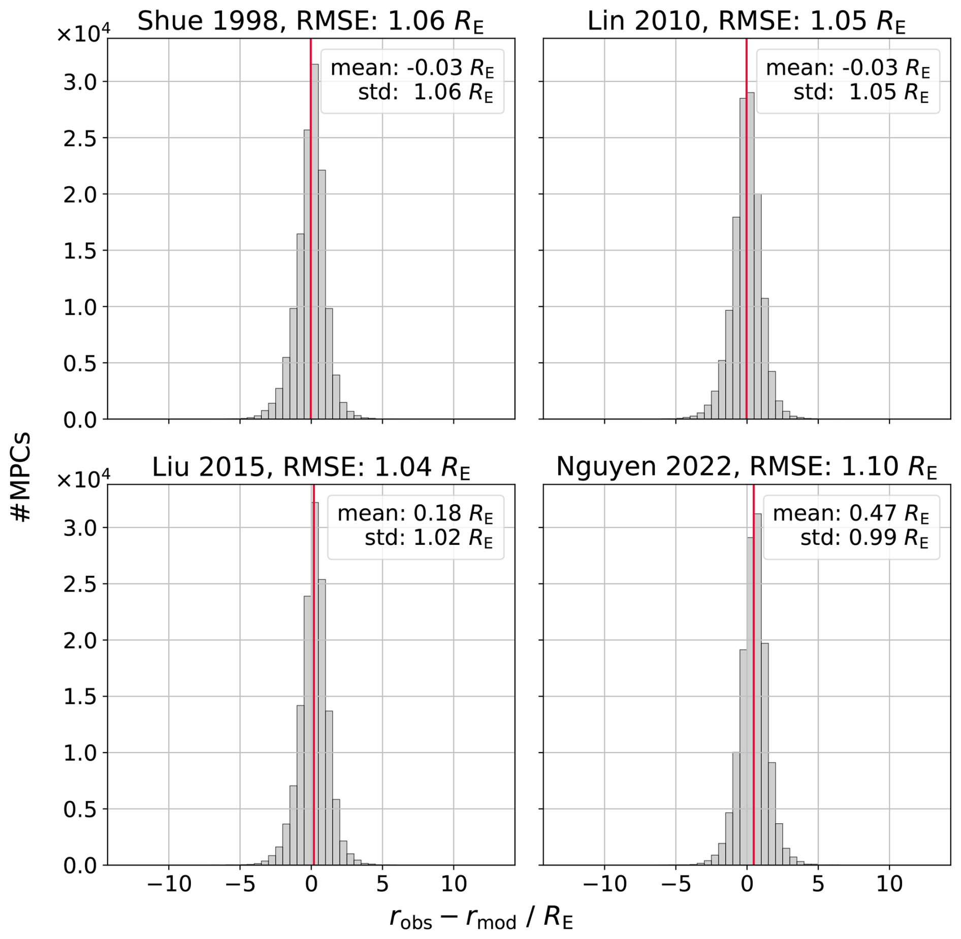
Figure 2 Δr distributions for four different magnetopause models, based on 133 045 dayside magnetopause crossings. The binsize is 0.5 R_E, the mean value is visualized by the red vertical line.

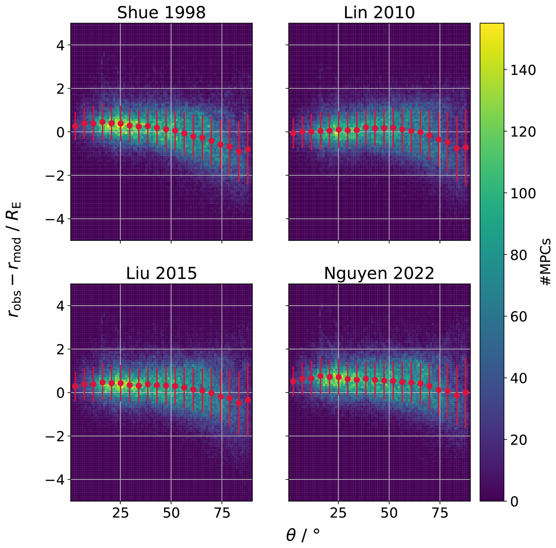
Figure 3 Heatmap of Δr over the zenith angle. Red dots with error bars mark the mean and standard deviation per bin of 4.5° zenith angle. The binsize is 1°×0.1 R_E. Approx. 200 outlying data points are not shown for each model.

3.2 Subsolar Region

In this study, magnetopause crossings with θ<30° are considered subsolar. A zenith angle smaller than 30° is also chosen by, e.g., Aghabozorgi Nafchi et al. (2024) to characterize the subsolar region, since then the magnetopause distance r_MP is very close to the subsolar standoff distance r₀ due to the approximately spherical shape of the magnetopause for low zenith angles. The number of usable MPCs is reduced the same way as for the full dayside magnetopause, resulting in 33 845 usable MPCs. Again, Δr is calculated for every crossing and every model. Figure 4 depicts the resulting distributions. The RMSE decreases for all models compared to the full dayside. Lin10 undergoes the largest improvement, while the Ng22 performance does not change much. Looking in the region of θ<30° in Fig. 3 further explains the positive mean value for every model (underestimation of the magnetopause distance). For the subsolar region, some models clearly perform better than others. While the standard deviation is similar for all models, the mean deviation drives the difference in RMSE. Interestingly, the standard deviation remains rather high at roughly 0.8 R_E with an improvement of approx. 20 % compared to the full dayside. The findings suggest, that albeit the different models make similar predictions regarding the subsolar standoff distance, they still are not able to quantify it accurately.

Grimmich et al. (2023b) computes the equivalent subsolar standoff distance for every MPC and calculates Δr with respect to the Sh98 model. Since in the subsolar region, r₀≈r_MP, the results are comparable specifically in that region. Grimmich et al. (2023b) gets a mean deviation of 0.36 R_E and a standard deviation of 0.76 R_E, which are nearly the same as in our investigation, although the analysis methods differ slightly. The performance comparison shows that in spite of more than two decades of advancement in magnetopause modeling, there remains little measurable improvement in the models' ability to accurately predict the magnetopause location.

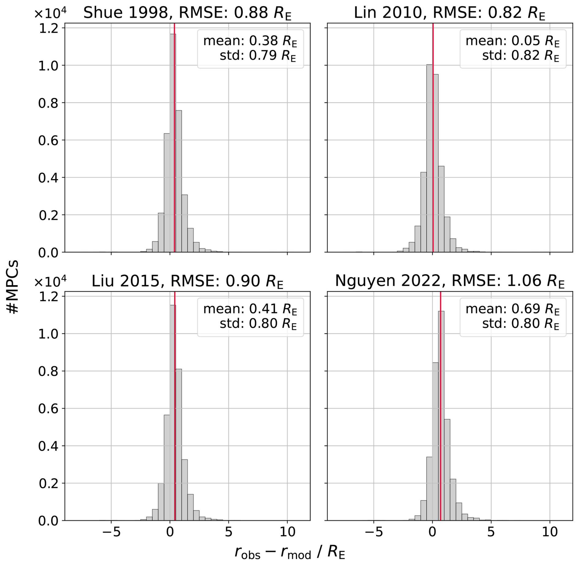
Figure 4 Δr distributions for four different magnetopause models, based on 33,845 magnetopause crossings in the subsolar region (θ<30°). The binsize is 0.5 R_E, the mean value is visualized by the red vertical line.

4 Parameter Relevance and Impact Evaluation

While the importance of the dynamic pressure on the magnetopause location is evident, the effect of the IMF is highly complex and probably not fully understood yet (see e.g. Wang et al., 2014; Lu et al., 2013; Aghabozorgi Nafchi et al., 2023). Additionally, apart from B_z, there is little consensus on which IMF parameters are most relevant for magnetopause modeling. Verigin et al. (2009) even find that the B_z component has no influence at all on the magnetopause location. It is also unclear weather the individual IMF components, the clock and cone angle or a combination of both is more suitable for magnetopause modeling. While Dušík et al. (2010) claim that the IMF cone angle plays a crucial role, Aghabozorgi Nafchi et al. (2023) focus on the clock angle of the IMF. Case and Wild (2013) on the other hand conclude that the clock angle has no influence on the radial magnetopause distance. That said, so far the Ng22 model is the only one of the presented models that includes the IMF clock angle. A new model developed by Aghabozorgi Nafchi et al. (2024) uses both the clock and cone angle as parameters. Němeček et al. (2020b) suggest to consider additional parameters to model the location of the magnetopause. While the authors claim that the $\mathrm{Na}/\mathrm{Np}$ ratio has no significant impact, the strength of Earth's magnetospheric currents does alter the magnetopause location. Additionally, the solar radio flux at 10.7 cm (Tapping and DeTracey, 1990; Tapping, 2013) is used as a proxy for the Sun's activity and the authors conclude that the inclusion of the parameter in magnetopause models would improve the prediction capabilities. Further, the influence of the ring current on the magnetopause location is investigated by, e.g., Machková et al. (2019) and Aghabozorgi Nafchi et al. (2024). Aghabozorgi Nafchi et al. (2024) use the corrected Dst index (Dst*) as a representative for the ring current. Additionally, Staples et al. (2020) connect the SYMH index to variations in observed and measured magnetopause standoff distance.

The main difficulty of choosing appropriate parameters lies in the fact that it is not easily distinguishable which magnetopause response originates from which parameter. Since most of the parameters are correlated or interconnected in some way, attributing effects to individual parameters is hardly possible. Moreover, the magnetopause configuration can appear similar despite differing external conditions. Conversely, under identical conditions, the magnetopause shape can still vary, introducing a degree of variability. Therewith, the initial step in constructing a new magnetopause model involves determining the key parameters that govern its shape and position.

4.1 Machine Learning Setup

Li et al. (2023) used a machine learning approach to find out which parameters are the most important for magnetopause modeling. However, the authors used MPCs from the whole dayside, a small dataset and a limited selection of parameters. Therefore, the same concept is applied again in this work on an extensive dataset.

ML algorithms are often treated as black boxes, where the internal decision-making process remains opaque. While the outputs can be insightful and empirically validated, the underlying reasons for these results are frequently unclear. This lack of interpretability makes it difficult to establish meaningful connections between input and output parameters, and thereby to extract insights into, for example, underlying physical relationships. To address the challenge of interpretability in machine learning models, particularly those treated as black boxes, various explainable AI (XAI) techniques have been developed. One of the most widely used approaches is based on Shapley values, a concept originally derived from cooperative game theory. Introduced by Shapley (1953), Shapley values provide a principled method to fairly distribute the ”payout” among players based on their individual contributions to the total outcome. In the context of machine learning, this framework has been adapted to quantify the contribution of each input feature to a model's prediction. By considering all possible combinations of features, Shapley values offer a theoretically grounded and model-agnostic approach to explain how and to what extent each input feature influences the output, thereby enabling a deeper understanding of the learned relationships and supporting scientific interpretation of complex models. However, the exact computation of Shapley values is computationally expensive, as it requires evaluating all possible subsets of input features - an operation with factorial complexity relative to the number of features. This becomes impractical for models with even a moderate number of inputs. To address this challenge, SHAP (SHapley Additive exPlanations), a Python package introduced by Lundberg and Lee (2017), provides efficient algorithms and approximations for estimating Shapley values in a tractable manner. The obtained value is called the SHAP value and is used in the place of the Shapley value in the following. SHAP performs well with tree based random forest ML algorithms (Lundberg et al., 2020). Therefore, the Python library XGBoost (Chen and Guestrin, 2016) is used to train a regressor model. The training data consists of 80 % of all MPCs, with the target value being the observed magnetopause distance r_obs. All but three hyperparameters of the XGB model are kept at their default values. The adjusted hyperparameters are the number of trees in the random forest (𝚗_𝚎𝚜𝚝𝚒𝚖𝚊𝚝𝚘𝚛𝚜=1000), the depth, i.e. number of decisions, of each tree (𝚖𝚊𝚡_𝚍𝚎𝚙𝚝𝚑=6), and the contribution of each tree, which also influences how conservative the model is and how it generalizes (𝚕𝚎𝚊𝚛𝚗𝚒𝚗𝚐_𝚛𝚊𝚝𝚎=0.05). The SHAP value is then evaluated for every parameter per available MPC.

4.2 Feature Importance

To get an overview of which parameters might be important for future magnetopause models, a regressor with 18 parameters is trained. The parameters are the dynamic and magnetic pressure, the AE and SYMH indices, the clock and cone angle, the components and the absolute value of the solar wind velocity and the IMF, the ion temperature, the $\mathrm{Na}/\mathrm{Np}$ ratio, the dipole tilt angle and the F10.7 solar flux. The zenith angle is limited to 30° to focus on the subsolar region. Because some parameters are missing for certain MPCs, the total number of usable crossings reduces to 18 787. Especially the $\mathrm{Na}/\mathrm{Np}$ ratio decreases the amount of usable MPCs, because it is only available for less than 50 % of all detected magnetopause crossings. Figure 5 shows a beeswarm plot of the obtained SHAP values for every parameter. The parameters are ordered in decreasing importance from top to bottom, where importance is quantified by the mean absolute value of all SHAP values per parameter and denoted as S(i) where i is the respective parameter. The color assigned to each data point reflects the value of its underlying parameter. As one can expect, the dynamic pressure is ranked as the most important parameter with S(p_dyn)=0.53 R_E. On its own, it accounts for a difference in r₀ exceeding 5 R_E, with higher values leading to magnetopause compression (indicated by low SHAP values), and lower values associated with expansion (high SHAP values). This is in good agreement with the literature and empirical models.

The following two parameters are the AE and SYMH indices (S(AE)=0.14 R_E, S(SYMH)=0.1 R_E), both capable of chaning the predicted value of r₀ up to about 2 R_E. As a general trend, the magnetopause moves inward for high parameter values. While the Dst and SYMH index have been used to model Earth's magnetosphere (Tsyganenko, 2013, and references therein), they did not get much attention for magnetopause modeling. Machková et al. (2019) investigate the influence of Dst* on the magnetopause standoff distance and find that the standoff distance decreases for increasing Dst*. A recent neural network model by Aghabozorgi Nafchi et al. (2024) uses Dst* as an input and exhibits the same dependency. Both findings agree with the SHAP values of the SYMH index in this investigation. To the best of our knowledge, the AE index has not been previously used in modeling the magnetopause location. However, our analysis clearly demonstrates that it may be a significant parameter that can potentially improve the model results.

The next important parameter is the F10.7 solar flux (S(F10.7)=0.09 R_E), which is a direct proxy of the solar activity. Long-term variations of the magnetopause due to the solar cycle are investigated by Němeček et al. (2016). The authors draw the conclusion that the F10.7 index does correlate with the magnetopause location. The derived SHAP values result in a similar conclusion.

Interestingly, the IMF magnitude B seems to be more important (S(B)=0.08 R_E) than the magnetic pressure, which is derived from it (S(p_mag)=0.05 R_E). Larger IMF strengths and therefore higher magnetic pressure shift the pressure balance between the sum of dynamic and magnetic pressure in the magnetosheath and the magnetic pressure from Earth's magnetic field closer to Earth, hence the negative SHAP values for high parameter values. This is consistent with magnetopause models such as Lin10 and Ng22, which use the sum of the dynamic and magnetic pressure. Although the magnetic pressure is significantly smaller than the dynamic pressure and is considered negligible by Němeček et al. (2020b), the SHAP values from our analysis suggest that it exerts a non-negligible influence – particularly when the IMF magnitude is used directly instead of the magnetic pressure.

Earth's dipole tilt angle γ is also ranked as an important parameter with an importance of S(γ)=0.07 R_E, justifying its use in many magnetopause models. Based on the SHAP values, our analysis underscores the importance of including the dipole tilt angle in magnetopause models. The effect of the tilt angle is larger in the high latitude and cusp regions, further away from the subsolar point. Still, SHAP values show that the tilt angle is also a crucial parameter for the low-latitude regime. Nguyen et al. (2022a) examines the influence of different IMF parameters on the shape and location of the magnetopause. One conclusion is that the IMF cone angle does not impact the subsolar standoff distance. However, the SHAP values suggest the opposite, with the parameter ranking fairly high, scoring an importance value of S(θ_cone)=0.06 R_E. Also, the feature value is systematic across most of the SHAP values. We therefore conclude that the cone angle has the potential to further enhance the quality of future magnetopause models. Grimmich et al. (2023b) finds that the cone angle is able to explain extreme deviations from theoretical to observed r₀, further underlining the importance of the parameter. In combination with the IMF magnitude, the two parameters cover the influence of the IMF in greater extend than the Sh98 and Lin10 models, which only use the B_z component.

The $\mathrm{Na}/\mathrm{Np}$ ratio is the only parameter covering the alpha particles in the solar wind. Previously discussed plasma parameters refer to protons only. Despite their lower abundance in the solar wind (∼5 %), alpha particles are nearly four times heavier than protons and thus can exert a non-negligible influence on the overall dynamic pressure of the solar wind, which is usually neglected. High values for $\mathrm{Na}/\mathrm{Np}$ have the potential to decrease the subsolar standoff distance by more than 0.5 R_E as indicated by the SHAP values. Němeček et al. (2020b) claim that the observed dependence of the magnetopause location on solar wind speed cannot be attributed to the contribution of alpha particles to the upstream pressure. Although subtle, the SHAP analysis ranks this parameter among the top contributors, assigning it an importance of $S\left(\mathrm{Na}/\mathrm{Np}\right)=\mathrm{0.06}{R}_{\mathrm{E}}$. A crucial restriction is that including the $\mathrm{Na}/\mathrm{Np}$ ratio roughly halves the amount of usable MPCs, since the parameter is available for only about 40 % of all crossings from the OMNI 1 min high resolution database. Using a lower time resolution (five minute or one hour averages) ups the percentage of usable MPCs, but decreases the significance of the parameter. It is therefore decided to keep the one minute time resolution to better reflect the impact of the parameter on the magnetopause position.

All remaining parameters have an importance score of less than 0.05 R_E and are considered less important for the magnetopause standoff distance. Furthermore, the ordering of features with low SHAP importance can fluctuate based on the underlying XGBoost model, or rather the composition of the training data, which are randomly selected 80 % of all MPCs. Still, the IMF B_z component and the clock angle rank low across different XGBoost models. Both parameters are used in previous magnetopause models or standoff distance parameterizations; especially the B_z component, which is generally believed to be an important parameter by, e.g., the aforementioned magnetopause models. While a correlation between SHAP value and B_z value is visible, the performed investigation indicates that the B_z component is not as important as widely believed, altering the standoff distance marginally. Also, the B_x components ranks higher than the B_z component for multiple different XGBoost models, further justifying the importance of the cone angle. The clock angle ranks as the lowest of all investigated parameters, supporting the conclusion of Case and Wild (2013).

On top of the discussed parameters, additional quantities have been investigated. They are not shown here since they are either not relevant (e.g. magnetosonic Mach number, plasma beta), or too closely connected to already investigated parameters (e.g. the proton density SHAP values carry the same information as the ones for the dynamic pressure).

The obtained results are somewhat difficult to compare to the ones by Li et al. (2023), because of a different underlying dataset (including the spatial coverage of MPCs), machine learning model, and parameter choice. Both studies conclude that the dynamic pressure and the IMF magnitude rank highest and the cone angle ranks higher than the clock angle. Additionally, the dependencies between SHAP value and feature value overlap with our results for most parameters. Still, Li et al. (2023) finds that the B_z component is more important than the B_x component and ranks high in general (S(B_z)=0.11 R_E). The differences in the results are possibly due to the mentioned differences in the analysis.

Based on the SHAP value investigation, the six most important parameters are selected for further use as inputs for a magnetopause model. The parameters are the dynamic pressure, the AE and SYMH indices, the IMF magnitude, Earth's dipole tilt angle and the IMF cone angle. Despite the F10.7 solar flux being ranked as fourth important parameter, it is not considered in the following. That is because later analysis shows that the inclusion of F10.7 does not significantly reduce the RMSE of the models. Therefore, the influence of F10.7 is believed to be already covered by other parameters, thus not contributing much additional information. As a possible seventh parameter, the alpha particle to proton ratio was considered. Given that including this parameter would significantly reduce the available training data, we ultimately chose not to incorporate it in magnetopause modeling. All other parameters ranked less important than the cone angle (S(i)<0.05 R_E) are also disregarded from further analysis.

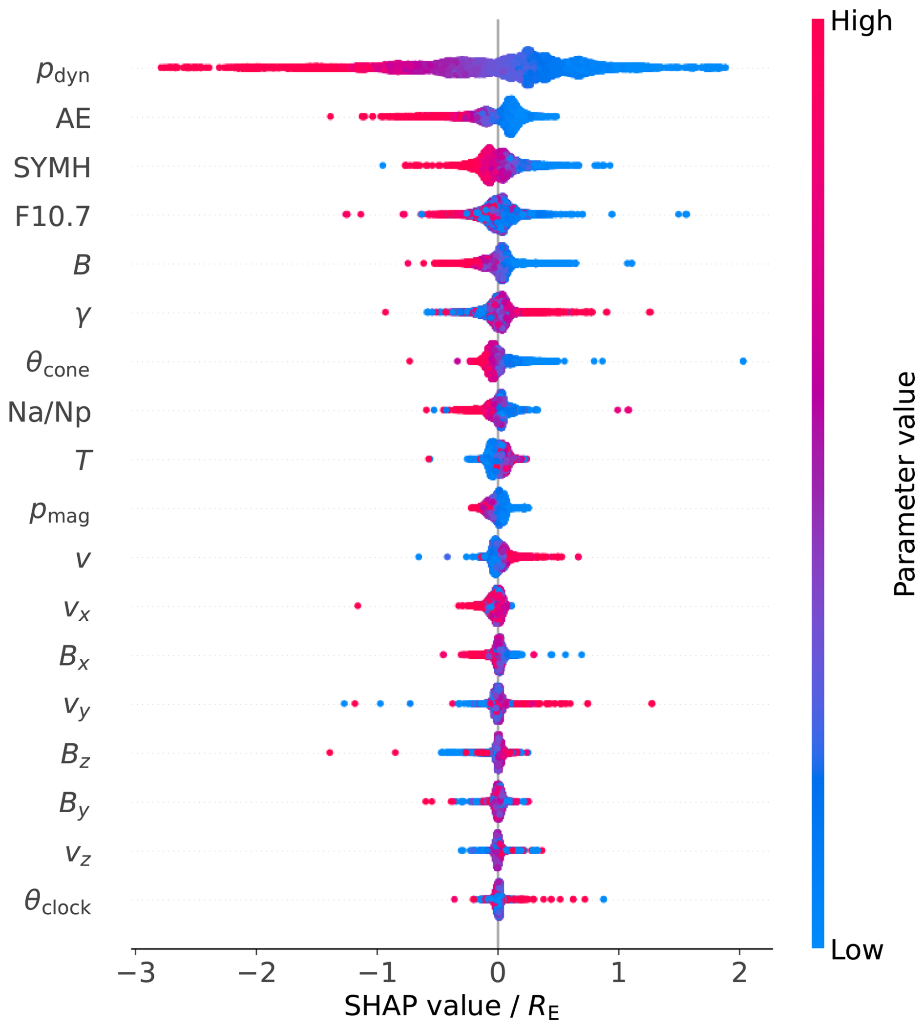
Figure 5 Beeswarm plot of the SHAP values for 18 selected parameters. 18,787 crossings from the subsolar region are analyzed.

4.3 Parameter Influence on r₀

SHAP values provide an overview of the influence on the magnetopause distance of individual parameters. Alternative visualization methods also enable a degree of quantitative analysis. However, to better understand the impact of individual parameters on the subsolar standoff distance, a second ML approach is utilized. A Support Vector Regression (SVR) model is trained using the scikit-learn Python module (Pedregosa et al., 2011) with the following nine input parameters: six parameters from the previous section identified as the most important, namely the solar wind dynamic pressure, the IMF cone angle and magnitude, the AE and SYMH indices, the dipole tilt angle, and a three-component n-vector, representing the position of each MPC. The vector is normalized and points from the center of the Earth to the respective MPC position. The target variable is the observed magnetopause distance. The maximal zenith angle is again limited to 30°, leaving a total of 32 667 MPCs. 80 % of the crossings are used to train the model, the remaining 20 % are the test set. SVR is a supervised machine learning algorithm that extends the principles of Support Vector Machines (SVM) to regression problems. SVR aims to find a function that approximates the relationship between input features and a continuous target variable while maintaining a margin of tolerance defined by the hyperparameter ε. Only data points with prediction errors larger than ε contribute to the cost function, promoting sparsity in the solution. The hyperparameter C controls the trade-off between model complexity and the degree to which deviations larger than ε are penalized; higher values of C allow the model to fit the training data more closely, at the risk of overfitting. The kernel coefficient γ_SVR defines the influence of individual training samples: lower values imply a smoother model, while higher values lead to more localized influence and greater model flexibility. Wang et al. (2013) utilize a SVR model to establish a global 3D magnetopause model, functioning as a proof of concept for the method of SVR. The authors used the solar wind dynamic pressure, the IMF B_z component and Earth's dipole tilt angle in combination with a n-vector as input parameters. The hyperparameter ε is set to 0, while C=20 and γ_SVR=1 are found by visual inspection of the resulting models. In this work, the optimal model parameters are found by hyperparmeter tuning to be ε=0.1, C=20 and γ_SVR=0.01. For SVR, it is important to standardize the input parameters and the target value by removing the mean and scaling to unit variance. The respective values used for scaling each parameter can be found in Table 1. After the prediction, the resulting r₀ values and the input features need to be scaled inversely. The trained SVR model has an RMSE of 0.68 R_E, calculated for the 32 667 subsolar MPCs. Therewith, the error is decreased by approx. 17 % with respect to the Lin10 model, the one with the smallest error of the compared models (refer Fig. 4). Note that the model is not able to make accurate predictions for parameter inputs outside the ranges specified in Table 1.

The dependency of r₀ on different parameters is depicted in Fig. 6 in form of Ceteris Paribus plots. In a Ceteris Paribus plot, all parameters but the one on the x-axis is kept constant at a given value. In this case, the mean value (see Table 1) of the respective parameters is chosen. Doing so allows to investigate the influence of each parameter independently. The n-vector is set to $(n_x,n_y,n_z)=(\mathrm{1},\mathrm{0},\mathrm{0})$, representing the subsolar point. The plot range of the abscissae is defined by the 1 % (99 %) quantile of the training data for the lower (upper) bound. All general trends of the individual parameters agree with the color-coding of the SHAP values from Fig. 5. Additionally, the ranges of the ordinates largely reflect the relative importance of the features, with p_dyn showing the widest range and less important parameters smaller ranges. The fact that two different ML approaches result in qualitatively similar results underscores the validity of the observed patterns and increases confidence in the interpretability of the models. It further suggests that the identified relationships are not model-dependent artifacts.

Figure 6 panel (a) shows the influence of the solar wind dynamic pressure on r₀. The typical non-linear decrease of r₀ with increasing p_dyn is present. A log-log representation of the same plot (not shown) reveals that the dependency is not linear, indicating that the relationship does not follow a power-law of the form $r_{\mathrm{0}}\propto p_{\mathrm{dyn}}^{-\mathrm{1}/k}$ with constant k, as assumed in all previously compared models. In fact, k is larger for low and high dynamic pressures (k>10 for p_dyn<1.4 nPa and p_dyn>9.6 nPa) and smaller for the intermediate dynamic pressure range (k<6 for $\mathrm{3}\mathrm{nPa}<p_{\mathrm{dyn}}<\mathrm{7.2}$ nPa). Aghabozorgi Nafchi et al. (2024) chose a similar approach to find the response of r₀ to different parameters and found k varying for different values of p_dyn too, likewise did Wang et al. (2013).

The dependence of the subsolar standoff distance on the AE index is shown in Fig. 6b. Specifically, r₀ decreases as AE increases. This trend aligns with established solar wind–magnetosphere coupling physics: elevated AE values correspond to increased substorm-related reconnection, which enhances magnetospheric current systems and erodes the dayside magnetopause (Tsurutani and Gonzalez, 1997). Therefore, less magnetic flux is present on the dayside during high AE intervals. The AE index may therefore capture magnetospheric processes that are not reflected by other parameters directly.

A high (low, meaning strongly negative) SYMH index is the result of a quiet (enhanced) ring current. The subsolar standoff distance decreases for high SYMH values, as shown in Fig. 6c. Aghabozorgi Nafchi et al. (2024) observe a similar relationship, but with the Dst* rather than the SYMH index, which reflects a related underlying principle, but do not discus possible reasons. We suggest that a stronger ring current is due to more particles being injected into the near–Earth magnetosphere. Therefore, the pressure just inside the magnetopause increases. To restore the pressure balance, the magnetopause has to move outward, explaining the identified relationship between SYMH and r₀.

High IMF magnitude corresponds to high magnetic pressure, pushing the magnetopause earthward. Despite the magnetic pressure being small in comparison to the dynamic pressure, it is included in more recent magnetopause models. The SHAP value analysis shows that instead of the magnetic pressure, the IMF magnitude has a more severe impact on the magnetopause standoff distance, visible in Fig. 6d. As expected, r₀ decreases with increasing IMF magnitude, agreeing with results from, e.g., Aghabozorgi Nafchi et al. (2024).

The influence of the dipole tilt angle is investigated by Liu et al. (2012), who performed MHD simulations for typical solar wind configurations. The authors conclude that the dipole tilt angle has little to no effect on the magnetopause position and shape for the equatorial magnetopause. The same conclusion is drawn by Aghabozorgi Nafchi et al. (2024), stating that the influence of the tilt angle is small and can therefore be neglected. Our analysis (see Figure 6e) shows that the typical influence of the dipole tilt angle is about 0.4 R_E, up to 1 R_E for some cases (Fig. 1), which is too much to be ignored. The relationship between r₀ and γ is similar to the two aforementioned studies. They find a symmetric dependency with the maximum value of r₀ at γ=0° (Aghabozorgi Nafchi et al., 2024) and a cosine relationship (Liu et al., 2012). In our case, the curve is also symmetric but peaks at $\mathit{\gamma }\approx -\mathrm{4}\mathit{°}$. Note that the exact functional form of the dependency in our case is influenced by the values of the other parameters. One observation is that with increasing dynamic pressure, the impact of other parameters reduces. This is due to the fact that the dynamic pressure is the main driver of the magnetopause location. If it is weak, other parameters have a greater impact and vice versa. Therefore, the impact of the dipole tilt angle varies with other parameters - not only in magnitude, but also in functional form (Wang et al., 2013).

Figure 6 panel (f) depicts the influence of the cone angle. Values near 0° correspond to radial IMF, Parker spiral configuration is at θ_cone≈45° and larger values reflect quasi perpendicular IMF at the subsolar point. The results indicate that the magnetopause is located farther from Earth under quasi-radial IMF conditions, while it moves closer under perpendicular IMF orientations. This is in good agreement with former studies (Dušík et al., 2010; Samsonov et al., 2012; Grygorov et al., 2017; Baraka et al., 2021; Aghabozorgi Nafchi et al., 2024).

Despite being classified as not important, the solar wind speed v shall be discussed briefly. SHAP values indicate increased r₀ with faster solar wind (ref. Fig. 5). According to p_dyn∝v² and r₀ decreasing with increasing dynamic pressure, the relation seems contradicting at first. However, faster solar wind usually is less dense, resulting in moderate dynamic pressure (Borovsky, 2020). Also, high solar wind speed increases the convection electric field and dayside reconnection and therewith the particle intake into the magnetosphere. The increased ring current results in an increase of the subsolar standoff distance, as discussed for the SYMH index. Lastly, fast solar wind often occurs at times of radial IMF, which in turn coincides with an extended magnetosphere. Li et al. (2023) find the same relationship between solar wind speed and magnetopause standoff distance, but do not discuss the potential reasons.

Table 1 Mean, standard deviation, and valid parameter ranges (lower and upper bounds) of the six parameters used to model the subsolar standoff distance.

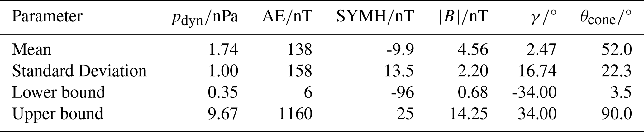
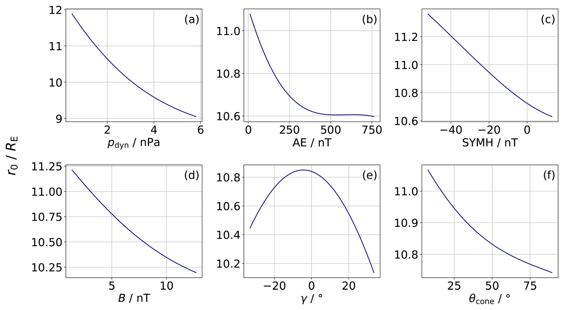
Figure 6 Ceteris Paribus plot of the subsolar standoff distance for each of the six non-positional parameters used to train the SVR model. Per panel, every parameter but the analyzed one is kept constant at the respective mean value. The n-vector has values of $(n_x,n_y,n_z)=(\mathrm{1},\mathrm{0},\mathrm{0})$, representing the subsolar point. The plot range is chosen to be from the 1 % to the 99 % quantile of each parameter.

4.4 On a Global ML Magnetopause Model

Our analysis shows that a machine learning approach is suitable to investigate the influence of certain drivers on the position of the subsolar magnetopause. On the MPC dataset at hand, the SVR model outperforms the established magnetopause models from literature regarding the accuracy of the prediction. Additionally, the influence of certain parameters reflects results from previous studies, showing that the approach has a potential to improve the understanding of magnetopause dynamics under varying solar wind conditions. This raises the question of whether a similar methodology could be employed to develop a global 3D magnetopause model, following examples set by, e.g., Wang et al. (2013).

To do so, a nine parameter SVR model is trained with in total 128 232 dayside MPCs (θ<90°). The input parameters and target value are the same as for the model discussed in the previous subsection. The trained model has an RMSE of 0.75 R_E, which is an improvement of more than 25 % compared to the best of the four compared models (ref. Fig. 2) and only slightly worse than the model for the subsolar region. A comparison between the SVR-predicted magnetopause shape and that of the Lin10 model (see Fig. A1) reveals significant discrepancies, especially in the y=0 plane. This is most likely due to the fact that the training dataset has only a few high latitude MPCs, covering, e.g., the cusps or polar regions. Consequently, the SVR algorithm struggles to accurately reproduce the magnetopause shape in those specific regions. Machine learning models are particularly effective at making predictions for parameters that lie within the parameter space seen during training. However, for uncovered or sparsely populated parameter space volumes, the model cannot predict the target variable accurately. This applies both to certain regions in space and to parameter combinations that are underrepresented in the training dataset. Since the majority of the MPCs lie close to the equatorial plane (with full longitudinal coverage on the dayside), this region is likely the most accurate region of the model. Comparing the equatorial plane with the Lin10 model shows a strong dawn-dusk asymmetry, where the dawn flank is up to 3 R_E closer to Earth than the dusk flank at the terminator. While the dawn–dusk asymmetry of Earth's magnetopause is an active area of research (Walsh et al., 2014; Baraka et al., 2021; Janda et al., 2024), the extent of the asymmetry continues to be a subject of debate. It therefore remains unclear whether the SVR model accurately represents the real magnetopause configuration, or whether the pronounced differences arise from artifacts in the data, such as orbital biases of the satellite missions.

Summarizing the findings, the discrepancies between our model and the Lin10 model are highest in the high latitude regions and on the dawn side, where a strong asymmetry is present. While discrepancies from established models are expected in the development of new magnetopause models, it is challenging to determine which model is more accurate based on visual inspection alone. Extensive hyperparameter tuning was performed on the SVR model to achieve an optimal trade-off between accuracy and overfitting. Doing so, the model is evaluated on unseen test data that has not been used for training the model. When plotting the residuals over the predicted value or individual parameters, no correlation is noticeable. The analysis also shows that the model performs equally well for different areas in space and over certain parameter ranges. Therewith, the SVR model is validated to the best of our abilities. The small RMSE of 0.75 R_E suggest good prediction capabilities. Subsequently, the ML approach, utilizing a SVR model, has the potential to model the dayside magnetopause more accurate than ever before. Nevertheless, the model can potentially lead to false predictions for certain cases, e.g., for uncommon (and therefore unseen during training) input parameter combinations (or parameters out of the bounds in Table 1), especially for the high latitude regions. We suggest that ML models based on the given dataset can be used to predict the equatorial region accurately, but shall be handled with care when investigating other regions and extreme inputs, as ML models often provide unphysical results when used outside of the bounds of the training data set (Zhelavskaya et al., 2021).

5 Parameterization of the Subsolar Standoff Distance

As an alternative to machine learning models, developing a novel parameterization of the subsolar standoff distance based on key identified parameters may be beneficial, as parameterization directly reveals which parameters contribute in which way and strength. Also, a simple equation may be able to better extrapolate to extreme values than a ML model. While previously developed magnetopause models frequently use a power law for the dynamic pressure and a hyperbolic tangent relationship for the B_z component, we decide on a second order polynomial representation for all parameters including cross and linear terms. The chosen six parameters are the same as for the subsolar SVR model: the dynamic pressure, the IMF magnitude, the AE and SYMH indices, the cone angle and the dipole tilt angle. The zenith angle is limited to 30° to only include subsolar crossings. Hence, 32 667 MPCs are used to fit the model. The input features are standardized by removing the mean and scaling to unit variance. Mean values and standard deviations are the same as mentioned in Table 1 of Sect. 4.3. The target value r₀ is not scaled and expressed in units of R_E. To fit the polynomial, the Python library sciki-learn is used. First, the input parameters are expanded into polynomial terms up to degree two with PolynomialFeatures and then fit by LinearRegression. The resulting 28 unique coefficients (a) have the unit of R_E and are represented in Fig. 7. The exact values are presented in Appendix B. A threshold based color coding is applied, with the threshold set to 0.03 R_E. Coefficients with an absolute value greater than the threshold are considered more important (colored in blue). The remaining coefficients are set equal to zero (colored in red). Doing so reduces the amount of coefficients from 28 to 14, effectively halving the complexity of the function. The explicit formula for r₀ is obtained by summing the products of the parameters corresponding to the cells colored in blue and the respective coefficient and is presented in Appendix B. Note that since the parameter values are scaled before fitting the equation, the input values must be scaled in the same manner.

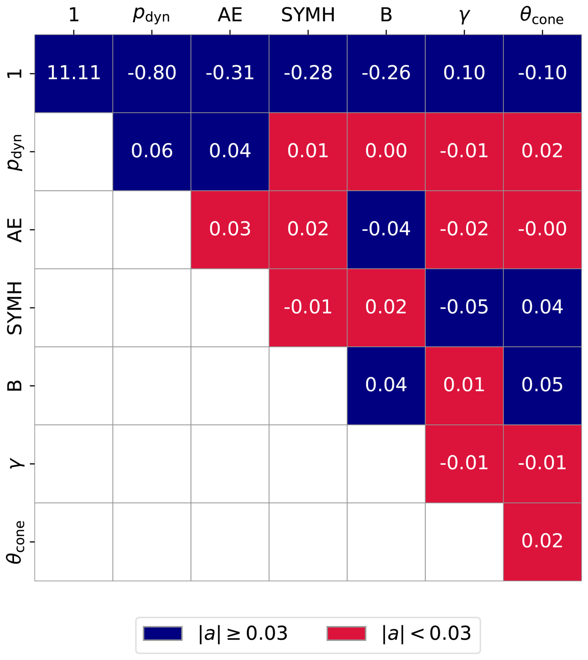
Figure 7 Coefficients of the fitted second-order polynomial for r₀. The matrix entries represent the polynomial coefficients: the first row contains the linear terms, the diagonal elements correspond to the quadratic terms, and the top-left cell denotes the bias (intercept) term. The remaining off-diagonal elements represent the cross terms. All coefficients are expressed in units of R_E. Values are color-coded based on a threshold of 0.03.

To justify the thresholding, the performances of the complete and simplified parameterization are compared. The complete formula predicts the magnetopause distance with a RMSE of 0.72 R_E (〈Δr〉 of zero, std(Δr)=0.72 R_E), while the simplified formula has a RMSE of 0.73 R_E (〈Δr〉=0.03 R_E, std(Δr)=0.73 R_E), showing that on average the prediction accuracy remains nearly unchanged even when using the simplified formula. This is further supported by the observation that the difference in calculated r₀ between parameterizations (complete vs. simplified) has a mean value of 0.03 R_E and a standard deviation of 0.12 R_E, indicating that the methods predict similar standoff distances also for individual cases. The threshold value of 0.03 is chosen to balance parameterization complexity with keeping the RMSE as small as possible. Increasing the threshold further reduces the amount of necessary parameters but increases the RMSE simultaneously. The RMSE of the parameterization is similar to the one obtained by the subsolar SVR model, showing that a simpler, non ML approach leads to similar prediction accuracy. At the same time, it might be an indication that a RMSE of 0.7 R_E is difficult to improve further. Still, this value is the lowest ever obtained on the applied dataset.

The cells colored in blue in Fig. 7 indicate important coefficients. It stands out that all coefficients for the linear terms (top row) are not set equal to zero. More specifically, the absolute values of the coefficients correspond to the order of parameter importance shown in Fig. 5 (ordered left to right from important to less important parameters in Fig. 7). Therewith, the method also seems to be able to quantify the parameter importance. The signs of the linear terms are consistent with the observed parameter influences; specifically, they match the slope directions of the curves in Fig. 6 and align with the color-coding of the SHAP values in Fig. 5.

The cells on the diagonal correspond to quadratic terms. Only the quadratic terms for the dynamic pressure and the magnetic field magnitude are included in the simplified formula. Doing so, the curves of the respective parameters resemble a power law representation more closely, which is how the dynamic pressure is usually used for r₀ parameterizations. Among others, the Lin10 model uses the sum of magnetic and dynamic pressure in a power law representation. Hence, it is reasonable to include a higher order term for the IMF magnitude too.

Almost all included cross terms have a contribution of either the AE or the SYMH index. While the exact physical meaning remains uncertain, it shows that the inclusion of the indices into the parameterization and magnetopause models is in general justified.

Higher order polynomials to parameterize r₀ have been investigated, but they do not decrease the RMSE enough to justify the increased parameterization complexity. Therefore, the polynomial degree is kept at two. Additionally, the dynamic pressure is not included in form of a power law to keep the procedure as simple as possible. Predefining the power law dependency might help to decrease the RMSE further. Adding more parameters to the equation also does not significantly lower the RMSE. The included parameters therewith cover the majority of information needed to predict the subsolar standoff distance accurately.

It has to be noted that, similar to the SVR model, the model does not extrapolate well. Due to, e.g., the coefficient of the quadratic dynamic pressure term being positive, r₀ would eventually increase artificially for large values of p_dyn, which is not physically motivated. In reality, the opposite is the case, where extreme dynamic pressures, e.g., due to the passage of interplanetary coronal mass ejections (ICMEs), strongly compress the magnetopause. To ensure correct predictions, we emphasize to use the model for the applicable parameter ranges specified in Table 1.

The presented parameterization use the AE and SYMH indices. While the parameters are crucial for accurate modeling of the subsolar standoff distance, they are not available in real time. An operational (nowcasting) version for r₀ parameterization, not using AE and SYMH, is presented in Appendix C.

6 Conclusions

In this work, an extensive dateset of Earth's magnetopause crossings has been used to (1) compare the prediction accuracy of four established magnetopause models for the dayside and subsolar regions; (2) determine which parameters are crucial for magnetopause modeling; (3) quantify the effect of each parameter on the subsolar standoff distance; and (4) develop a new parameterization of the subsolar standoff distance with a second order polynomial and six input parameters.

The most important findings can be summarized as follows:

1. The magnetopause models by Shue et al. (1998), Lin et al. (2010), Liu et al. (2015), and Nguyen et al. (2022c) yield similar accuracy in predicting the dayside magnetopause, with RMSEs slightly exceeding 1 R_E. For the subsolar region (zenith angle smaller than 30°), the RMSEs decrease but stay greater than 0.8 R_E. Despite its relatively simple geometric formulation, the Sh98 model performs on par with more recent and structurally complex models. This observation indicates that advances in magnetopause modeling over the past two and a half decades have yielded only incremental gains in magnetopause position prediction precision.

2. SHAP values computed from a trained XGBoost regressor model are highly valuable in revealing which parameters are capable to significantly alter the position of Earth's magnetopause. The analysis provides new insights into the roles of several parameters, including both those previously used in magnetopause modeling and those that have not been traditionally considered.

3. The geomagnetic AE and SYMH indices are identified as important parameters to include in a magnetopause model. They both are closely linked to the magnetopause standoff distance and can explain variations of up to 1 R_E. The AE index has not been considered for magnetopause models so far - we suggest that it should be in the future. Recent studies propose the use of Dst* as a model parameter. However, we opt to include the SYMH index instead, due to its higher time resolution and practically equivalent physical interpretation.

4. Contrary to common belief, the instantaneous IMF B_z component does not seem to be a crucial parameter concerning the magnetopause standoff distance. It is therefore not included in the r₀ parameterization. We point out that other representations of B_z, such as its minimum or mean value over a period of time prior to the MPC may play a more important role than B_z itself, which should be investigated in the future. The effect of dayside reconnection, the process B_z is responsible for, is possibly covered by the geomagnetic indices or a combination of other parameters, making B_z redundant. Instead, the IMF B_x component is classified as an important parameter. It ranks higher than B_z in the SHAP value analysis and is also indirectly represented by the IMF cone angle. Since the cone angle ranks even higher than B_x, it is chosen as an input parameter for our model.

5. Parameter influence on r₀ is studied trough SHAP values and a SVR model. Both methods yield consistent results, which are generally in line with previously published studies and theoretical predictions. The solar wind dynamic pressure has the biggest influence on the magnetopause standoff distance, but does not follow an exact power law. Increasing AE and SYMH indices both reduce r₀; the same applies to the IMF magnitude. Our analysis further shows that an increasing IMF cone angle θ_cone decreases r₀. Former studies showed that radial IMF (θ_cone=0° for purely radial conditions) corresponds to larger standoff distances, which is in agreement with our findings. For average solar wind and IMF conditions we find r₀ peaking when Earth's dipole tilt angle γ is approx. −4° and decreasing for increasing $\left|\mathit{\gamma }\right|$. Past studies also show a symmetric dependency, but with the maximum r₀ at γ=0°. We note that the exact dependence relies on the other input parameters, which should be studied in the future.

6. Despite promising results achieved by machine learning regression models, a global magnetopause model based on, e.g., SVR is not feasible with the available MPC dataset. This is due to the lack of magnetopause crossings in the high latitude regime including the cusp region and the nightside. Sparse data in those regimes lead to inaccurate predictions. Additionally, ML models do not extrapolate well on unseen data during training and are therefore only valid in a certain parameter range. We propose however, that ML models are highly valuable when used correctly, e.g., for a limited sector as the subsolar region or close to the equatorial plane on the dayside.

7. A second order polynomial with six input parameters is suitable to fit the subsolar standoff distance for a given range of each input parameter. Input parameters are the dynamic pressure, AE and SYMH indices, IMF magnitude, Earth's dipole tilt angle, and the IMF cone angle. The polynomial has a RMSE of 0.72 R_E, which is better than that of any of the four magnetopause models compared in this work. To verify the model performance, future work should benchmark the model on an independent MPC data set. The polynomial allows for a reduction in complexity by setting half of the coefficients (14 of 28) equal to zero while keeping the RMSE and prediction capability almost unchanged. The coefficients of the linear terms also reflect the same order of parameter importance previously found by SHAP value analysis.

Despite the valuable insights gained from this study, several issues remain to be addressed. Similar to most other established magnetopause models, the parameterization of r₀ is static, meaning that no time dependency whatsoever is included. While, e.g., Gu et al. (2025) and Nguyen et al. (2022b) propose methods for dynamic magnetopause models, the topic is covered sparsely in the literature. As an intermediate step, it would be a consideration to time shift individual parameters, like the AE index, before they are used in the model. Typically it takes some time (in the order of minutes to hours, depending on the parameter) for the magnetopause to respond to a change in the environment. However, brief analysis showed that no significant improvement is achieved by timeshifting different input parameters. Another problem with magnetopause modeling is the uncertainty of, e.g., the IMF or the dynamic pressure at the bow shock (Walsh et al., 2019; Di Matteo and Sivadas, 2022). Regardless of best effort to propagate space weather parameters from the L1 point to Earth's bow shock, Aghabozorgi Nafchi et al. (2024) claim that the intrinsic inaccuracy of magnetopause models stems from insufficient knowledge of the upstream solar wind parameters. This could also be the case for this work, possibly explaining why the RMSE of our parameterization remains at approx. 0.7 R_E. Future magnetopause models should account for the inherent variability of the magnetopause position by providing not only a point prediction, but also an estimated range within which the boundary is likely to reside. Wang et al. (2013) applied this concept in a SVR model, providing one possible way of incorporating the variability of the magnetopause. Building on such approaches, future research should prioritize probabilistic modeling and uncertainty quantification to better reflect the dynamic and inherently variable nature of the magnetopause. Additionally, models need to be more robust in handling extreme input conditions from, e.g., ICMEs, which are able to compress the magnetopause to otherwise unseen distances. This is particularly important in light of upcoming missions like the Solar Wind Magnetosphere Ionosphere Link Explorer (SMILE) (Wang et al., 2025), which aims to provide continuous global observations of the magnetopause and will benefit from models that can account for its dynamic and uncertain nature.

Appendix A: SVR Dayside Model Compared to Lin10

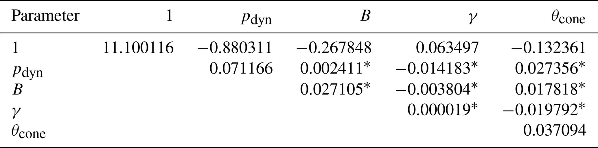
Figure A1 displays the Lin10 and a custom SVR model in three planes for the same MPC. A detailed description can be found in the caption.

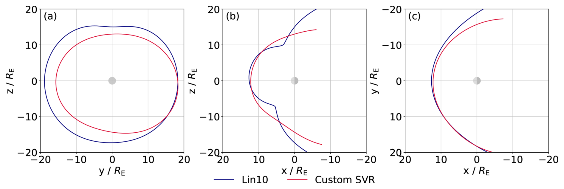
Figure A1 An exemplary comparison of the SVR full-dayside model and the Lin10 model under identical input parameters in (a) the terminator, (b) the y=0, and (c) the equatorial plane in AGSE coordinates. Input conditions are: p_dyn=0.77 nPa, $\mathit{\gamma }=-\mathrm{11}\mathit{°}$ for both models, p_mag=0.004 nPa, B_z=0.6 nT additionally for Lin10, and B=3.22 nT, AE=54 nT, $\mathrm{SYMH}=-\mathrm{5}\mathrm{nT}$, θ_cone=23.5° additionally for the SVR model. Note the strong differences in magnetopause shape in the high latitude regions in panels (a) and (b). Also, an extensive dawn-dusk asymmetry is present for the SVR model, visible in panels (a) and (c).

Appendix B: Equation of the Polynomial Model

The model equation of the subsolar standoff distance is as follows:

$$\begin{array}{ll}{\displaystyle }{r}_{\mathrm{0}}=& {\displaystyle }\mathrm{0.062766}{p}_{\mathrm{dyn}}^{\mathrm{2}}+{\mathrm{0.029063}}^{*}{\mathrm{AE}}^{\mathrm{2}}-{\mathrm{0.005244}}^{*}{\mathrm{SYMH}}^{\mathrm{2}}\\ {\displaystyle }& {\displaystyle }+\mathrm{0.036025}{B}^{\mathrm{2}}-{\mathrm{0.007827}}^{*}{\mathit{\gamma }}^{\mathrm{2}}+{\mathrm{0.024278}}^{*}{\mathit{\theta }}_{\mathrm{cone}}^{\mathrm{2}}\\ {\displaystyle }& {\displaystyle }+\mathrm{0.042863}{p}_{\mathrm{dyn}}\mathrm{AE}+{\mathrm{0.014235}}^{*}{p}_{\mathrm{dyn}}\mathrm{SYMH}\\ {\displaystyle }& {\displaystyle }+{\mathrm{0.003292}}^{*}{p}_{\mathrm{dyn}}B-{\mathrm{0.011979}}^{*}{p}_{\mathrm{dyn}}\mathit{\gamma }\\ {\displaystyle }& {\displaystyle }+{\mathrm{0.021987}}^{*}{p}_{\mathrm{dyn}}{\mathit{\theta }}_{\mathrm{cone}}+{\mathrm{0.018708}}^{*}\mathrm{AE}\mathrm{SYMH}\\ {\displaystyle }& {\displaystyle }-\mathrm{0.043601}\mathrm{AE}B-{\mathrm{0.016090}}^{*}\mathrm{AE}\mathit{\gamma }\\ {\displaystyle }& {\displaystyle }-{\mathrm{0.000336}}^{*}\mathrm{AE}{\mathit{\theta }}_{\mathrm{cone}}+{\mathrm{0.017716}}^{*}\mathrm{SYMH}B\\ {\displaystyle }& {\displaystyle }-\mathrm{0.045112}\mathrm{SYMH}\mathit{\gamma }+\mathrm{0.037957}\mathrm{SYMH}{\mathit{\theta }}_{\mathrm{cone}}\\ {\displaystyle }& {\displaystyle }+{\mathrm{0.006229}}^{*}B\mathit{\gamma }+\mathrm{0.045304}B{\mathit{\theta }}_{\mathrm{cone}}\\ {\displaystyle }& {\displaystyle }-{\mathrm{0.014665}}^{*}\mathit{\gamma }{\mathit{\theta }}_{\mathrm{cone}}-\mathrm{0.804452}{p}_{\mathrm{dyn}}\\ {\displaystyle }& {\displaystyle }-\mathrm{0.307622}\mathrm{AE}-\mathrm{0.276234}\mathrm{SYMH}\\ {\displaystyle }& {\displaystyle }-\mathrm{0.256840}B+\mathrm{0.097598}\mathit{\gamma }\\ \text{(B1)}& {\displaystyle }& {\displaystyle }-\mathrm{0.099100}{\mathit{\theta }}_{\mathrm{cone}}+\mathrm{11.105453}.\end{array}$$

Note that the unit of r₀ is R_E and the input parameters have no unit since they have been transformed using the respective quantities given in Table 1. Values marked with * are set to 0 by the threshold of 0.03 R_E.

Appendix C: Operational version of the r₀ parameterization

The parameterization presented in Sect. 5 enables retrospective reconstruction of the subsolar standoff distance based on known solar wind conditions, IMF, and geomagnetic activity. For the purpose of forecasting r₀ under in operational settings, it is beneficial to utilize a parameterization that does not rely on geomagnetic indices, but only on solar wind and IMF quantities. The same approach as described in Sect. 5 is utilized to obtain the coefficients shown in Fig. C1 (more decimal places in Table C1). The figure is in the same style as Fig. 7. The parameterization predicts the standoff distance with a RMSE of 0.76 R_E (mean of Δr equal to zero) when all 15 terms are included, which is slightly worse than the model including the geomagnetic indices. Reducing the complexity to 7 coefficients based on the threshold of 0.03 leads to a RMSE of 0.77 R_E, which is only marginally worse than the complete model, and close to the performance of the Lin10 model in the subsolar region despite its simplified form. The coefficient values are similar to the ones of the model including AE and SYMH. However, the cone angle seems to be more important such that the corresponding quadratic term is also above the threshold. Comparing the predictions for r₀ across the two different parameterizations (including the indices and not) shows that their difference has a mean of zero and a standard deviation of 0.24 R_E. To conclude, the full formula is likely more accurate, but using the parameterization without AE and SYMH gives a good first estimate.

Figure C1 Coefficients of the fitted second-order polynomial for r₀. Same style as Fig. 7.

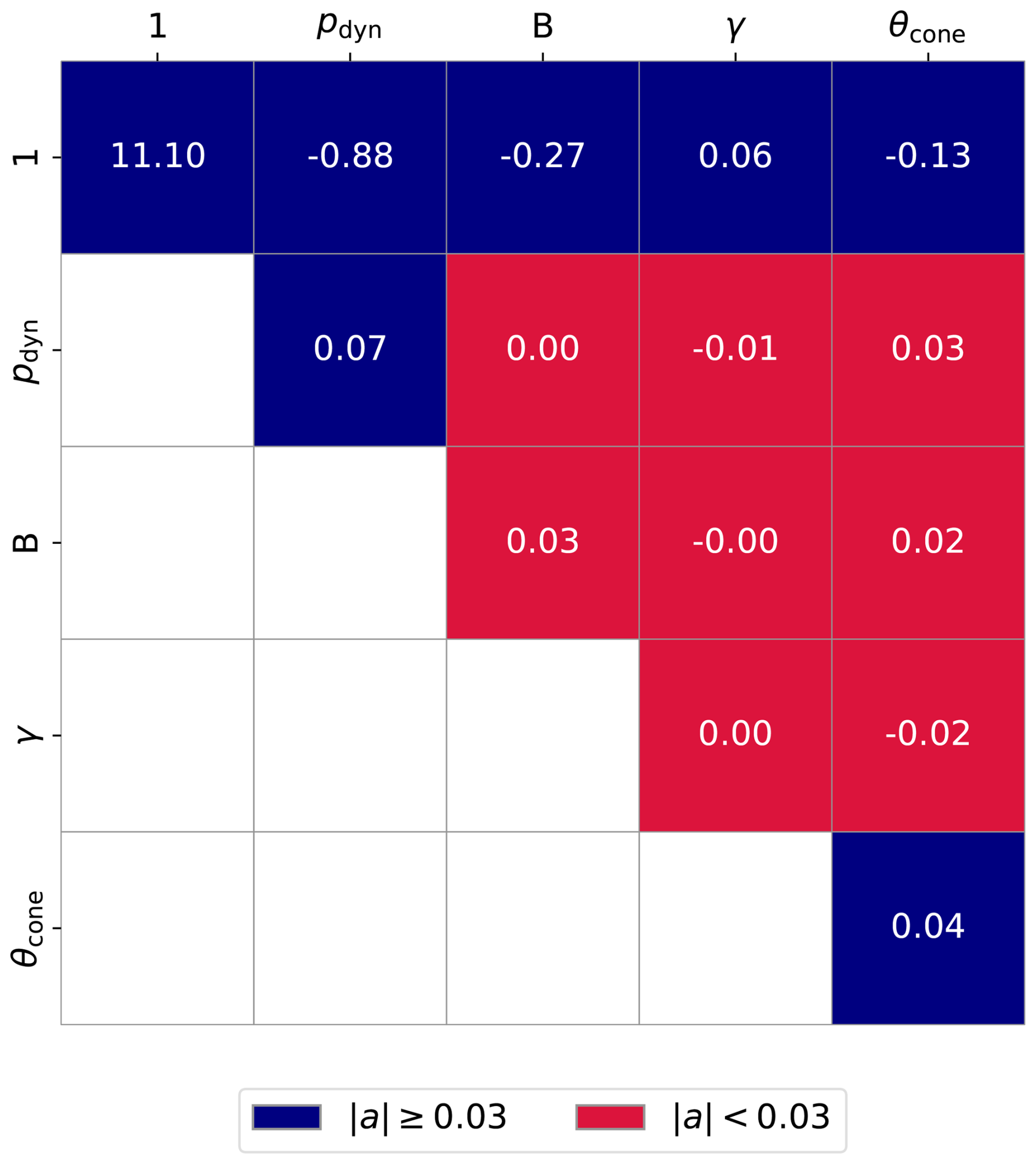
Table C1 Same coefficients as in Fig. C1 but with more decimal places. In units of R_E.

Values marked with ^* are set to 0 by the threshold of 0.03 R_E.