Global inductive magnetosphere-ionosphere- thermosphere coupling

The ionosphere forms the inner boundary of near-Earth space, where collisionless space plasma transitions into a partially ionized gas that interacts with the neutral atmosphere through collisions. Conventional models for magnetosphere-ionosphere (MI) coupling use an electric circuit framework, where an electric potential is calculated from the current continuity equation on a thin spherical shell that represents the ionosphere. This approach, founded in the E,j (electric field and current density) paradigm, contrasts with the approach used to study plasmas in other regions of cosmos, where the magnetic field B and plasma velocity v are treated as fundamental variables (the B,v paradigm). Since traditional MI coupling models also neglect induction by setting $\partial \mathit{B}/\partial t=\mathrm{0}$, they omit the dynamic processes by which B evolves, leaving the global MI coupling process arguably poorly understood. To advance our understanding of MI coupling, we present a new global model of the 2D ionosphere that incorporates induction, with B as the primary variable. This model accommodates arbitrary ionospheric conductance, neutral wind patterns, and realistic main magnetic field geometries. Simulations reveal the complex nature of the induction process over a few seconds to several minutes. The induction timescales depend on the magnitudes and spatial scales of conductance, neutral wind, imposed magnetic field perturbations, and main magnetic field geometry. We simulate for the first time how low-latitude Sq currents and electric fields emerge through induction. Our model has the potential to replace existing MI coupling modules in magnetospheric simulation codes, offering both a truly global solution, and the inclusion of induction in the coupled system dynamics.

1 Introduction

The magnetosphere constitutes the vast region of space where Earth's magnetic field has a dominating influence, a comet-shaped region that extends to about 10 R_E in the sunward direction, with a much longer tail on the nightside. Beyond the magnetosphere's outer boundary is the solar wind, which shapes it and powers most of its dynamics, including phenomena such as geomagnetic storms and auroral displays. The inner boundary of the magnetosphere is the ionosphere, where space plasma overlaps and interacts with the neutral atmosphere. Collisions between the charged particles of the plasma and neutrals in the ionosphere lead to exchanges of momentum and energy when the two fluids move relative to each other.

To our knowledge, all global simulations of the magnetosphere (Tóth et al., 2012; Zhang et al., 2019; Sorathia et al., 2020; Von Alfthan et al., 2014) use the same principle for coupling to the ionosphere: Field-aligned currents (FACs) are mapped along the main magnetic field of the Earth from the inner boundary of the magnetospheric simulation domain, typically a few Earth radii (R_E, set to 6371.2 km in this work), to a 2D spherical shell that represents the ionosphere. The incident FAC is used in the current continuity equation, along with prescribed electric conductivities and neutral winds, to solve for an electric potential (Merkin and Lyon, 2010; Ridley et al., 2004; Ganse et al., 2025) which serves as the inner boundary condition for the magnetosphere simulations. Earthward of the inner boundary, the potential depends on the neutral winds and assumptions about interhemispheric coupling (Maute et al., 2021; Richmond and Maute, 2014). In existing implementations, the potential is treated independently in the two polar hemispheres, and separated from the low latitudes by a boundary condition at some fixed latitude. This circuit-based approach, relating electric fields, conductivities, and currents via the so-called Ionospheric Ohm's law, has a long tradition in ionospheric physics (see, e.g., reviews by Richmond, 2016; Leake et al., 2014), and is derived from the momentum equations of electrons, ions, and neutrals, together with important assumptions for each of them.

In the conventional magnetosphere-ionosphere coupling schemes described above, the electric field E is represented as the gradient of a scalar potential, which implies that it is curl-free, and that $\partial \mathit{B}/\partial t=\mathrm{0}$ according to Faraday's law. In this work, we do not make this assumption, but we still neglect displacement currents, $\partial \mathit{E}/\partial t=\mathrm{0}$. While it is true that the rotational part of E is often small compared to the potential part of the field, it has been observed to be significant in some cases (Madelaire et al., 2024). Importantly, the lack of induction conceals the physical processes that drive ionospheric electrodynamics. The widespread use of this approximation has led to the idea that field-aligned currents set up an electric field, or that electric fields penetrate from higher altitudes, and drive convection and currents across magnetic field lines. This concept has been challenged in a series of papers arguing that instead of treating E and j as primary (the E,j paradigm), B and v should be seen as the primary variables, while E and j are derived (Vasyliūnas, 2001, 2012; Vasyliūnas and Song, 2005; Vasyliūnas, 2005; Parker, 1996). In the B, v paradigm the electric field and currents are understood as natural consequences of plasma convection and magnetic field deformations propagating from the magnetosphere, emphasizing the dynamic coupling between the magnetosphere and the ionosphere rather than viewing electric fields as externally imposed drivers.

Laundal et al. (2024) recently presented a simple conceptual model, a thought experiment in which the ionosphere is flat, the main magnetic field is vertical, the neutral winds are zero, and the dynamics is resolved in a single horizontal dimension. Their purpose was to elucidate the physical process of how the magnetosphere drives ionospheric dynamics, but the restrictive simplifications make it difficult to directly apply their model in a realistic scenario. In this paper, we extend the model by treating the ionosphere as a 2D spherical shell, and allowing arbitrary main magnetic field geometry, neutral wind, and horizontal gradients in all quantities. The resulting model can, in principle, replace the magnetostatic magnetosphere-ionosphere coupling scheme in conventional global magnetospheric models. Incidentally, our B,v-based approach can also be solved in steady state, in which case it reduces to the conventional magnetostatic approach. However, unlike conventional magnetostatic solvers, our model is truly global, with no boundaries that disconnect high- and low-latitude regions.

In Sect. 2 we explain the basic concept of our approach, starting from Maxwell's equations and the Generalized Ohm's law in 3D. In Sect. 3 we discuss simplifying assumptions, including the projection onto a 2D spherical shell, that reduces the computational complexity. Special attention is given to the boundary conditions, which are defined by the magnetic field above and below the ionosphere, represented with spherical harmonics. Section 4 presents example simulation results. We discuss the results, implications, and limitations in Sect. 5. Section 6 concludes the paper.

2 Basic Theory of Inductive Ionospheric Dynamics

In this section we present the basic equations of the inductive magnetosphere-ionosphere coupling scheme used in this paper. Our approach is inspired by Vasyliūnas (2012) and Chap. 9.5 in Parker (2007). It is related to a number of previous simulation studies in which the equations given below are solved in various 1D and 2D geometries (Tu and Song, 2016, 2019; Dreher, 1997; Otto and Zhu, 2003; Laundal et al., 2024). Here we present the equations for a 3D ionosphere. In the next section, we present the simplified equations that model the ionosphere as a 2D spherical shell, along with the approach used to define the boundary conditions.

The induction equation, or Faraday's law, is

$$\begin{array}{}\text{(1)}& {\displaystyle \frac{\partial \mathit{B}}{\partial t}}=-\mathrm{\nabla }\times \mathit{E}.\end{array}$$

To integrate this equation in time, the electric field E must be defined. We consider it to be given by the Generalized Ohm's law (Leake et al., 2014),

$$\begin{array}{}\text{(2)}& \mathit{E}={\displaystyle \frac{{\mathit{\sigma }}_{\mathrm{H}}\mathit{j}\times \widehat{\mathit{b}}+{\mathit{\sigma }}_{\mathrm{P}}\widehat{\mathit{b}}\times \left(\mathit{j}\times \widehat{\mathit{b}}\right)}{{\mathit{\sigma }}_{\mathrm{H}}^{\mathrm{2}}+{\mathit{\sigma }}_{\mathrm{P}}^{\mathrm{2}}}}-\mathit{u}\times \mathit{B}+\mathit{F},\end{array}$$

where u is the neutral wind, $\widehat{\mathit{b}}$ is the unit vector in the direction of the magnetic field, j is the electric current density, and σ_P and σ_H are Pedersen and Hall conductivities, respectively. This equation is derived from the momentum equations for ions and electrons. The vector F includes contributions from inertia, pressure gradients, gravity, and the magnetic field-aligned component of E. For a detailed derivation of this equation, see Leake et al. (2014). When F=0, the remaining terms in the momentum equations represent the Lorentz force and the momentum exchange with neutrals via collisions; and Eq. (2) represents the relationship between E and j when these two forces balance. In the following, we will assume that F=0. Pressure gradients and inertia are important to consider at high altitudes but become relatively less important in the E-region, where the collisional coupling between plasma and neutrals is strongest (Brekke, 2013). Furthermore, the conductivity along the magnetic field lines can be assumed to be large, implying that any electric field in the direction of the field lines is quickly equilibrated, which implies that $\mathit{B}\cdot \mathit{E}=\mathrm{0}$. The effects of pressure gradients and gravity are generally considered to be small, although their impacts are sometimes detectable (Alken, 2016; Laundal et al., 2019).

The Generalized Ohm's law and the Ionospheric Ohm's law are fundamentally the same equation, differing only in the variable being solved for: E for the Generalized Ohm's law or j for the Ionospheric Ohm's law. For F=0 the Ionospheric Ohm's law is (e.g., Brekke, 2013)

$$\begin{array}{}\text{(3)}& \mathit{j}={\mathit{\sigma }}_{\mathrm{P}}(\mathit{E}+\mathit{u}\times \mathit{B})+{\mathit{\sigma }}_{\mathrm{H}}\widehat{\mathit{b}}\times (\mathit{E}+\mathit{u}\times \mathit{B})+j_{\parallel }\widehat{\mathit{b}}.\end{array}$$

The conductivities primarily depend on plasma density and on the collision frequencies between the plasma species and neutrals (e.g., Strangeway, 2012). The collision frequencies, in turn, depend on temperature (Schunk and Nagy, 2009). The time evolution of density, momentum, and temperature are described by the continuity, momentum, and energy equations, respectively (Dreher, 1997; Otto and Zhu, 2003; Tu and Song, 2016; Laundal et al., 2024). In this paper, we assume that the density and temperature, and hence conductivity, are given, and that both ion and electron inertia can be neglected. Thus, the only equation we need to integrate in time is Faraday's law.

We obtain a closed set of equations by replacing the current density using Ampère's law in the quasi-static approximation,

$$\begin{array}{}\text{(4)}& \mathit{j}={\displaystyle \frac{\mathrm{1}}{{\mathit{\mu }}_{\mathrm{0}}}}\mathrm{\nabla }\times \mathit{B},\end{array}$$

and choosing appropriate boundary conditions for B. Equations (1), (2), and (4) can then be combined to describe the evolution of the magnetic field as a function of the magnetic field itself. The electric field can be retrieved at any time from Eq. (2) and the currents from Eq. (4), but, as pointed out by Parker (1996), they do not dictate the dynamics. It is possible but computationally expensive to evolve Faraday's law in 3D. In the next section, we derive the ionospheric induction equation for a 2D spherical shell, along with other simplifying assumptions that we use in our numerical simulation.

3 Dynamic MIT Coupling With 2D Ionosphere

In this section, we describe how we use Eqs. (1), (2), and (4) for a 2D spherical shell at radius r=R that represents the ionosphere. Since the collisional interaction between ions and neutrals peaks in the E-region, this region dominates the ionospheric response in any height-integrated description. Since F in this equation only becomes important outside the E-region (Brekke, 2013), we will neglect it here. In addition we will neglect the continuity and energy equations, which means that, as in conventional magnetosphere-ionosphere coupling schemes, the conductivities, which are functions of density and temperature (Schunk and Nagy, 2009), must be considered as given. Future iterations of the model may include all these effects as it is conceptually straightforward but computationally more expensive to evolve the fluid moments in time together with Faraday's law (Tu and Song, 2016).

Above the 2D ionosphere, we assume ideal MHD and that the magnetic field is force-free, which means that $\mathit{B}\times (\mathrm{\nabla }\times \mathit{B})=\mathbf{0}$. That is, all currents are field-aligned in this region. Below the ionosphere, we assume that there are no currents, so that the magnetic field is curl-free and can be expressed as a gradient of a scalar potential. These assumptions lead to a 3D description of the magnetic field above and below the ionosphere, described in more detail later in this section. The geometry is illustrated in Fig. 1. In this figure, which is to scale, the ionosphere looks like a thin blue line at about 110 km altitude, but is actually a contour plot of a typical Pedersen conductivity. Here, the Pedersen conductivity is based on measurements taken at a single geographic location using the EISCAT incoherent scatter radar on Svalbard, but the values are plotted across all latitudes to illustrate the radial dependence relative to a 2D cross-section of the Earth. This shows that the 2D assumption is reasonable on large scales.

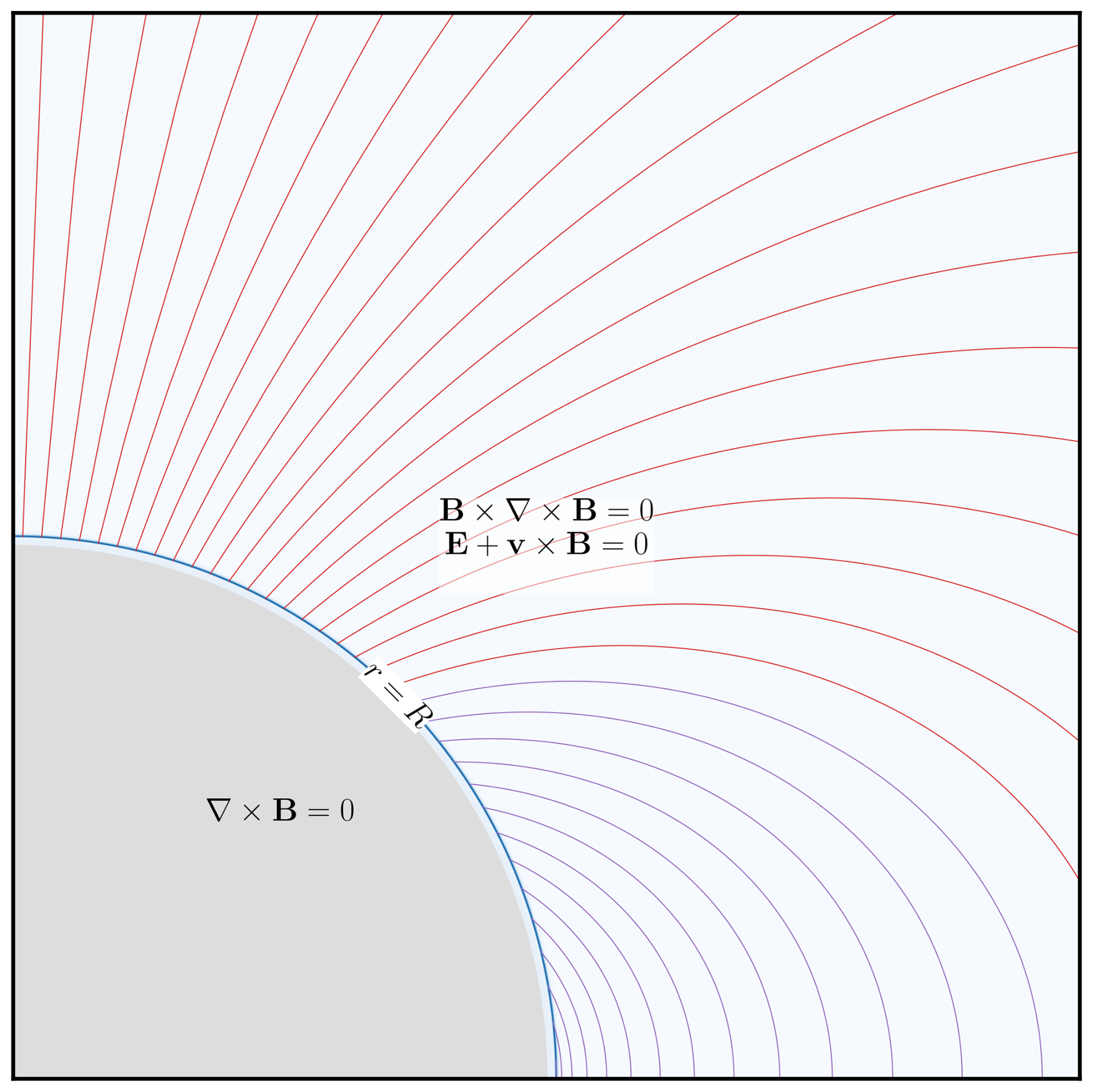
Figure 1 Cross section of the Earth, ionosphere, and inner magnetosphere (gap region) shown to scale. The ionosphere appears as a blue line but is in fact a linear color scale contour plot of a typical height profile of the Pedersen conductivity, highlighting the appropriateness of a 2D treatment. We simulate the radial component of the magnetic field B on the spherical surface at radius r=R, but the magnetic field is defined everywhere using the assumptions indicated in the figure. Above the ionosphere, we assume that the magnetic field is force-free ($\mathit{B}\times \mathrm{\nabla }\times \mathit{B}=\mathrm{0}$) and that it is frozen-in with the plasma, which moves at velocity v. Below the ionosphere, the magnetic field is assumed to be curl-free.

From magnetic flux conservation, the radial component of the magnetic field must be continuous across the ionosphere, which means that the radial component B_r must be the same as the ionosphere (located at r=R) is approached from above or from below. In our 2D model it will only be necessary to consider the radial component of Faraday's law,

$$\begin{array}{}\text{(5)}& {\displaystyle \frac{\partial B_r}{\partial t}}=-(\mathrm{\nabla }\times \mathit{E})\cdot \widehat{\mathit{r}}.\end{array}$$

The horizontal part of the electric field E_S can be expressed by projecting Eq. (2) on the horizontal plane by making the cross product with $\widehat{\mathit{r}}$ from the left and right: ${\mathit{E}}_{\mathrm{S}}=\widehat{\mathit{r}}\times \mathit{E}\times \widehat{\mathit{r}}$. The symmetry of the operation allows us to omit brackets, as the result is independent of the order of the cross products. Neglecting F we get

$$\begin{array}{}\text{(6)}& {\mathit{E}}_{\mathrm{S}}=\widehat{\mathit{r}}\times \left[{\displaystyle \frac{{\mathit{\sigma }}_{\mathrm{H}}\mathit{j}\times \widehat{\mathit{b}}+{\mathit{\sigma }}_{\mathrm{P}}\widehat{\mathit{b}}\times \left(\mathit{j}\times \widehat{\mathit{b}}\right)}{{\mathit{\sigma }}_{\mathrm{P}}^{\mathrm{2}}+{\mathit{\sigma }}_{\mathrm{H}}^{\mathrm{2}}}}-\mathit{u}\times \mathit{B}\right]\times \widehat{\mathit{r}}.\end{array}$$

To represent the ionosphere as a thin sheet at r=R, we treat its radial dependence as a delta function. In this formulation, the local conductivities are replaced by height-integrated conductances Σ_H,P, and we introduce the corresponding sheet current density J_S. A detailed derivation of this thin-sheet formulation from the ionospheric Ohm's law is given in Appendix A.

$$\begin{array}{}\text{(7)}& \begin{array}{rl}{\mathit{E}}_{\mathrm{S}}& =\widehat{\mathit{r}}\times \left[{\displaystyle \frac{{\mathrm{\Sigma }}_{\mathrm{H}}{\mathit{J}}_{\mathrm{S}}\times \widehat{\mathit{b}}+{\mathrm{\Sigma }}_{\mathrm{P}}\widehat{\mathit{b}}\times \left({\mathit{J}}_{\mathrm{S}}\times \widehat{\mathit{b}}\right)}{{\mathrm{\Sigma }}_{\mathrm{P}}^{\mathrm{2}}+{\mathrm{\Sigma }}_{\mathrm{H}}^{\mathrm{2}}}}-\mathit{u}\times \mathit{B}\right]\times \widehat{\mathit{r}}\\ & =\widehat{\mathit{r}}\times \left[{\mathit{\eta }}_{\mathrm{H}}{\mathit{J}}_{\mathrm{S}}\times \widehat{\mathit{b}}+{\mathit{\eta }}_{\mathrm{P}}\widehat{\mathit{b}}\times \left({\mathit{J}}_{\mathrm{S}}\times \widehat{\mathit{b}}\right)-\mathit{u}\times B_r\widehat{\mathit{r}}\right]\times \widehat{\mathit{r}}.\end{array}\end{array}$$

In the last line, we introduced the height-integrated resistances

$$\begin{array}{}\text{(8)}& {\displaystyle }{\mathit{\eta }}_{\mathrm{P}}={\mathrm{\Sigma }}_{\mathrm{P}}/\left({\mathrm{\Sigma }}_{\mathrm{H}}^{\mathrm{2}}+{\mathrm{\Sigma }}_{\mathrm{P}}^{\mathrm{2}}\right)\text{(9)}& {\displaystyle }{\mathit{\eta }}_{\mathrm{H}}={\mathrm{\Sigma }}_{\mathrm{H}}/\left({\mathrm{\Sigma }}_{\mathrm{H}}^{\mathrm{2}}+{\mathrm{\Sigma }}_{\mathrm{P}}^{\mathrm{2}}\right).\end{array}$$

The radial component of the current does not appear in our 2D projection of E. This can be understood by expressing the 3D current system in our model as $\mathit{j}=\mathit{\delta }(r-R){\mathit{J}}_{\mathrm{S}}+H(r-R)j_{\parallel }\widehat{\mathit{b}}$, where δ is the Dirac delta function and H is the Heaviside step function (1 for r≥R and 0 for r<R). In this expression, j_r appears only in the last term, which represents the magnetic field-aligned component of j, which is not included in Eq. (7) because of the cross product with $\widehat{\mathit{b}}$.

To replace the sheet current density, we use the jump condition for the magnetic field across the spherical shell sheet current (or 2D Ampère's law),

$$\begin{array}{}\text{(10)}& {\mathit{J}}_{\mathrm{S}}={\displaystyle \frac{\mathrm{1}}{{\mathit{\mu }}_{\mathrm{0}}}}\widehat{\mathit{r}}\times \mathrm{\Delta }\mathit{B},\mathrm{\Delta }\mathit{B}={\mathit{B}}^{+}-{\mathit{B}}^{-},\end{array}$$

where the superscript “+” signifies the limit of the magnetic field as r approaches R from above, and superscript “−” signifies the limit from below. The cross product with $\widehat{\mathit{r}}$ implies that only the horizontal components of the magnetic field are involved in this equation.

Equations (5), (7), and (10) form, with the boundary conditions and input discussed below, a closed set of equations, in which B_r evolves as a function of the magnetic field itself, similar to the 3D equations presented in Sect. 2. In combining these equations we introduce another simplifying and very useful assumption: That the perturbation magnetic field is so small that it does not significantly change the geometry of the magnetic field. This corresponds to a linearization of the equations. From this point onward, we refer to the main field as B₀, with unit vector components b_r,b_θ, and b_ϕ, and perturbations as B with components B_r,B_θ, and B_ϕ. Eq. (5) can then be written as

$$\begin{array}{}\text{(11)}& \begin{array}{rl}{\displaystyle \frac{\partial B_r}{\partial t}}& ={\displaystyle \frac{\mathrm{1}}{r\sin \mathit{\theta }}}\left(\begin{array}{cc}\frac{\partial }{\partial \mathit{\varphi }}& -\frac{\partial }{\partial \mathit{\theta }}(\sin \mathit{\theta }\cdot )\end{array}\right)\\ & [{\displaystyle \frac{\mathrm{1}}{{\mathit{\mu }}_{\mathrm{0}}}}\left(\begin{array}{cc}{\mathit{\eta }}_{\mathrm{P}}\left(b_{\mathit{\varphi }}^{\mathrm{2}}+b_r^{\mathrm{2}}\right)& -{\mathit{\eta }}_P{b}_{\mathit{\theta }}{b}_{\mathit{\varphi }}+{\mathit{\eta }}_{\mathrm{H}}{b}_r\\ -{\mathit{\eta }}_P{b}_{\mathit{\theta }}{b}_{\mathit{\varphi }}-{\mathit{\eta }}_{\mathrm{H}}{b}_r& {\mathit{\eta }}_{\mathrm{P}}(b_{\mathit{\theta }}^{\mathrm{2}}+b_r^{\mathrm{2}})\end{array}\right)\left(\begin{array}{c}-\mathrm{\Delta }{B}_{\mathit{\varphi }}\\ \mathrm{\Delta }{B}_{\mathit{\theta }}\end{array}\right)\\ & -B_{\mathrm{0}}\left(\begin{array}{c}-b_{\mathit{\varphi }}{u}_{\mathrm{r}}+b_{\mathit{r}}{u}_{\mathit{\varphi }}\\ -b_{\mathit{r}}{u}_{\mathit{\theta }}+b_{\mathit{\theta }}{u}_r\end{array}\right)],\end{array}\end{array}$$

where we have used Eqs. (7)–(10) to express the evolution of B_r in terms of the magnetic field, resistances, magnetic field geometry, and neutral wind. In the neutral wind term, we neglect the magnetic field perturbation since its contribution is very small compared to the main field contribution. This is the equation that we integrate in time to model the ionospheric dynamics. If needed, the horizontal electric field E_S can be retrieved by evaluating the expression in square brackets (equivalent to Eq. 7). The top row of the expression in square brackets refers to the θ component and the bottom row refers to the ϕ component.

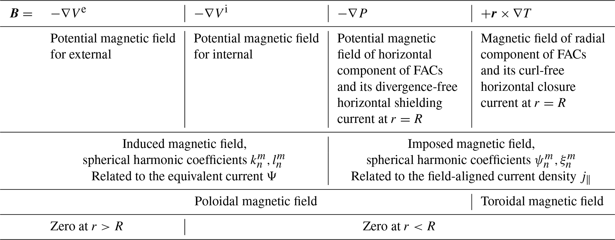
It remains to specify the components of ΔB, which consists of the magnetic field immediately above (B⁺) and below (B⁻) the ionosphere, according to Eq. (10). Below the ionosphere, this is straightforward: Since there are no currents there, the magnetic field is a potential field, and its potential satisfies Laplace's equation. To determine the solution, we integrate Eq. (5) in time to obtain $B_r(R,\mathit{\theta },\mathit{\varphi })$, which then serves as a boundary condition for the Laplace equation. We return to this in more detail in Sect. 3.1. Above the ionosphere, the situation is more complex. In addition to an induced part similar to the one below, there is also an imposed magnetic field. The imposed field is determined by solving the steady-state ideal MHD equations under the assumption of a force-free magnetic field, with boundary conditions set by specified field-aligned currents at high latitudes and constraints from interhemispheric coupling along magnetic field lines at low latitudes. This is discussed in detail in Sect. 3.2. We thus decompose the magnetic field into induced and imposed parts. The imposed field is zero below the ionosphere, while both parts contribute above it. Each part can be described in terms of different current systems: The induced part corresponds to a horizontal, divergence-free sheet current at r=R, referred to as the equivalent current. The imposed part, on the other hand, is associated with field-aligned currents. These relationships are discussed in more detail below.

In the above equations, we need only the horizontal component of the electric field E_S. At r≥R, the vertical component of the electric field can be retrieved from the assumption that the parallel component of E is zero:

$$\begin{array}{}\text{(12)}& \mathit{E}\cdot {\mathit{B}}_{\mathrm{0}}=\mathrm{0}\Rightarrow E_r=-\left(E_{\mathit{\theta }}{b}_{\mathit{\theta }}+E_{\mathit{\varphi }}{b}_{\mathit{\varphi }}\right)/b_r.\end{array}$$

Likewise, the sheet current at r=R (Eq. 10) can be connected to the full 3D current density at r>R by first using the current continuity equation to determine $j_r=-{\mathrm{\nabla }}_{\mathrm{S}}\cdot {\mathit{J}}_{\mathrm{S}}$, with ∇_S the horizontal (surface) gradient defined as

$$\begin{array}{}\text{(13)}& {\mathrm{\nabla }}_{\mathrm{S}}=\mathrm{\nabla }-\widehat{\mathit{r}}{\displaystyle \frac{\partial }{\partial r}},\end{array}$$

and then the force-free assumption to reconstruct the full current vector at r>R:

$$\begin{array}{}\text{(14)}& \mathit{j}\times {\mathit{B}}_{\mathrm{0}}=\mathbf{0}\Rightarrow \mathit{j}=j_r/b_r\widehat{\mathit{b}}.\end{array}$$

In the next subsections we define the induced and imposed parts of the magnetic field, together with their corresponding currents, using spherical harmonics. We also describe how this decomposition is related to the more conventional decomposition into poloidal and toroidal parts.

3.1 The Induced Magnetic Field

Below the ionosphere j=0, which means that the magnetic field is curl-free and can be expressed as $\mathit{B}(r<R)=-\mathrm{\nabla }V$, where the magnetic potential V obeys the Laplace equation ∇²V=0. The solution can be expanded in spherical harmonics (see e.g., Sabaka et al., 2013 and Olsen, 1997)

$$\begin{array}{}\text{(15)}& \begin{array}{rl}{\mathit{B}}_{\mathrm{ind}}^{\mathrm{e}}& =-\mathrm{\nabla }{V}^{\mathrm{e}}\\ & =-\mathrm{\nabla }\left(R\sum _{n,m}{\left({\displaystyle \frac{r}{R}}\right)}^n{P}_n^m\right(\mathit{\theta }\left)\right[q_n^m\cos \left(m\mathit{\varphi }\right)\\ & +s_n^m\sin \left(m\mathit{\varphi }\right)\left]\right),\end{array}\end{array}$$

where the superscript “e” signifies that the magnetic field corresponds to a current that is “external” with respect to the observation radius r. Above the ionosphere, the situation is more complicated, because there the magnetic field is a superposition of induced and imposed parts. The imposed part is discussed in detail below. The induced part of the magnetic field at r>R is, by definition, the part that satisfies the Laplace equation. The solution is

$$\begin{array}{}\text{(16)}& \begin{array}{rl}{\mathit{B}}_{\mathrm{ind}}^{\mathrm{i}}& =-\mathrm{\nabla }{V}^{\mathrm{i}}\\ & =-\mathrm{\nabla }\left(R\sum _{n,m}{\left({\displaystyle \frac{R}{r}}\right)}^{n+\mathrm{1}}{P}_n^m\right(\mathit{\theta }\left)\right[g_n^m\cos \left(m\mathit{\varphi }\right)\\ & +h_n^m\sin \left(m\mathit{\varphi }\right)\left]\right),\end{array}\end{array}$$

where the superscript “i” signifies that the field corresponds to an “internal” current. For B_r, which defines the induced part of the magnetic field, to be continuous across r=R we must have that

$$\begin{array}{}\text{(17)}& \underset{r\to R^{-}}{lim}{\displaystyle \frac{\partial }{\partial r}}{V}^{\mathrm{e}}=\underset{r\to R^{+}}{lim}{\displaystyle \frac{\partial }{\partial r}}{V}^{\mathrm{i}}\end{array}$$

which leads to the following relationships between the coefficients $q_n^m,s_n^m$ and $g_n^m,h_n^m$ (Sabaka et al., 2013)

$$\begin{array}{}\text{(18)}& n{q}_n^m=-(n+\mathrm{1})g_n^m,n{s}_n^m=-(n+\mathrm{1})h_n^m.\end{array}$$

These relationships are enforced by defining the coefficients $k_n^m$ and $l_n^m$,

$$\begin{array}{}\text{(19)}& \mathit{\{}{k}_n^m,l_n^m\mathit{\}}\equiv -{\displaystyle \frac{\mathrm{1}}{n+\mathrm{1}}}\mathit{\{}{q}_n^m,s_n^m\mathit{\}}={\displaystyle \frac{\mathrm{1}}{n}}\mathit{\{}{g}_n^m,h_n^m\mathit{\}},\end{array}$$

with these forms chosen to simplify subsequent mathematical relationships. Inserting Eq. (19) into Eqs. (15) and (16) we obtain that the total induced magnetic field B_ind can be written as B_ind=∇V, where

$$\begin{array}{}\text{(20)}& V=\left\{\begin{array}{ll}-R\sum _{n,m}(n+\mathrm{1}){\left(\frac{r}{R}\right)}^n{P}_n^m\left(\mathit{\theta }\right)\left[k_n^m\cos \left(m\mathit{\varphi }\right)+l_n^m\sin \left(m\mathit{\varphi }\right)\right],& r<R,\\ R\sum _{n,m}n{\left(\frac{R}{r}\right)}^{n+\mathrm{1}}{P}_n^m\left(\mathit{\theta }\right)\left[k_n^m\cos \left(m\mathit{\varphi }\right)+l_n^m\sin \left(m\mathit{\varphi }\right)\right],& r>R.\end{array}\right.\end{array}$$

Note that V is undefined at r=R, but Eq. (17) implies that its radial derivative is defined also at this point. In other words, the radial component B_r of the magnetic field at r=R can be obtained through

$$\begin{array}{}\text{(21)}& B_r(R,\mathit{\theta },\mathit{\varphi })=\sum _{n,m}n(n+\mathrm{1})P_n^m\left(\mathit{\theta }\right)\left[k_n^m\cos \left(m\mathit{\varphi }\right)+l_n^m\sin \left(m\mathit{\varphi }\right)\right].\end{array}$$

Equations (15)–(18) describe a one-to-one relationship between B_r and the induced part of the magnetic field on both sides of the ionosphere. Given an initial condition for B_r, the coefficients $k_n^m$ and $l_n^m$ can be determined by integrating Eq. (11) and inverting the spherical harmonic representation in Eq. (21). Once these coefficients are known, the magnetic field immediately below the ionosphere (B⁻) and the induced part of the magnetic field immediately above the ionosphere (${\mathit{B}}_{\mathrm{ind}}^{+}$) can be reconstructed using Eq. (20). The imposed part of the magnetic field immediately above the ionosphere is yet to be defined.

The horizontal sheet current at r=R that is equivalent with B_ind can be found with Ampère's law, Eq. (10). Inserting the magnetic field we get the equivalent current, which can be expressed as

$$\begin{array}{}\text{(22)}& {\mathit{J}}_{\mathrm{eq}}=\widehat{\mathit{r}}\times {\mathrm{\nabla }}_{\mathrm{S}}\mathrm{\Psi },\end{array}$$

where the equivalent current function Ψ can be identified from ${\mathit{J}}_{\mathrm{eq}}=\frac{\mathrm{1}}{{\mathit{\mu }}_{\mathrm{0}}}\widehat{\mathit{r}}\times \mathrm{\Delta }{\mathit{B}}_{\mathrm{ind}}$, giving (see, e.g., Laundal et al., 2018)

$$\begin{array}{}\text{(23)}& \mathrm{\Psi }=-{\displaystyle \frac{R}{{\mathit{\mu }}_{\mathrm{0}}}}\sum _{n,m}(\mathrm{2}n+\mathrm{1})P_n^m\left(\mathit{\theta }\right)\left[k_n^m\cos \left(m\mathit{\varphi }\right)+l_n^m\sin \left(m\mathit{\varphi }\right)\right].\end{array}$$

The equivalent current is important because it can be derived from ground magnetometer measurements of magnetic field perturbations (Kamide et al., 1981; Untiedt and Baumjohann, 1993; Laundal et al., 2015). If the main magnetic field is assumed to be radial ($b_{\mathit{\theta }}=b_{\mathit{\varphi }}=\mathrm{0}$), the equivalent current equals the divergence-free part of J_S (Vasyliūnas, 2007).

3.2 The Imposed Magnetic Field

While the induced magnetic field has a one-to-one relationship with the equivalent current, the imposed magnetic field is a force-free magnetic field confined to r>R and has a one-to-one relationship to the field-aligned currents. As in the conventional MI coupling approach, we make the simplifying assumption that field-aligned currents map instantaneously between the magnetosphere and the upper boundary of the ionosphere, through what Merkin and Lyon (2010) term the gap region. At low latitudes, we assume that field-aligned currents instantaneously connect the hemispheres along magnetic field lines such that the electric field matches at conjugate points, in keeping with the assumption of a force-free magnetic field and ideal MHD, $\mathit{E}+\mathit{v}\times \mathit{B}=\mathbf{0}$, above the ionosphere (Hesse et al., 1997). An equivalent statement is that the Alfvén speed is so high that any j×B force is immediately removed, or shifted to the magnetospheric and ionospheric boundaries, so that the magnetic field in the gap region at all times is relaxed in a force-free configuration. This is of course a simplification, and a physical description of the Alfvén wave propagation through the gap region has been studied by e.g. Lotko (2004) and Wright (1996).

As for any divergence-free vector field we can write the imposed magnetic field in terms of poloidal and toroidal parts (Sabaka et al., 2013; Olsen, 1997; Backus, 1986),

$$\begin{array}{}\text{(24)}& {\mathit{B}}_{\mathrm{imp}}=\mathit{P}+\mathit{T},\end{array}$$

where the toroidal part $\mathit{T}=\mathit{r}\times \mathrm{\nabla }T$ is related to the radial current density and the poloidal part P is related to the horizontal part of the field-aligned current density. The toroidal scalar T can be expanded in terms of spherical harmonics (e.g., Olsen, 1997, Laundal et al., 2016, and Fillion et al., 2023):

$$\begin{array}{}\text{(25)}& T=\left\{\begin{array}{ll}\sum _{n,m}{P}_n^m\left(\mathit{\theta }\right)\left(\frac{R}{r}\right)\left[{\mathit{\psi }}_n^m\cos \left(m\mathit{\varphi }\right)+{\mathit{\xi }}_n^m\sin \left(m\mathit{\varphi }\right)\right],& r>R,\\ \mathrm{0},& r<R\end{array}\right.\end{array}$$

and the associated radial current density immediately above the ionosphere is:

$$\begin{array}{}\text{(26)}& j_r=-{\displaystyle \frac{\mathrm{1}}{R{\mathit{\mu }}_{\mathrm{0}}}}\sum _{n,m}n(n+\mathrm{1})P_n^m\left(\mathit{\theta }\right)\left[{\mathit{\psi }}_n^m\cos \left(m\mathit{\varphi }\right)+{\mathit{\xi }}_n^m\sin \left(m\mathit{\varphi }\right)\right].\end{array}$$

Thus, if we know j_∥ globally, we can find $j_r=b_r{j}_{\parallel }$ and ${\mathit{\psi }}_n^m$ and ${\mathit{\xi }}_n^m$, and hence T.

There are two aspects that make it somewhat complicated to calculate B_imp: (1) In MI coupling applications j_∥ is given at high latitudes, but not at low latitudes. The global pattern of j_∥, and thus the coefficients ${\mathit{\psi }}_n^m$ and ${\mathit{\xi }}_n^m$, must instead be specified through a combination of prescribed current patterns at high latitudes and the set of interhemispheric coupling constraints at low latitudes mentioned previously. We return to this in detail in Sect. 3.2.1. (2) The poloidal magnetic field P is a function of the horizontal part of the field-aligned current density in the entire volume at r>R, even if we only evaluate it immediately above R. In our model, this field encompasses the contribution from the horizontal part of the field-aligned currents at r>R and a divergence-free horizontal shielding current in the ionosphere that ensures that P is zero below the ionosphere. This shielding current is constructed as part of the imposed system in our decomposition and modifies the poloidal component of the imposed magnetic field above the ionosphere so that its radial component is zero at the ionosphere boundary. In Sect. 3.2.2 we describe how the shielding current can be calculated from the coefficients ${\mathit{\psi }}_n^m$ and ${\mathit{\xi }}_n^m$.

Before proceeding, we clarify a potential source of confusion in our terminology. We assume that the imposed magnetic field is contained above the ionosphere and describe induction as the process that allows magnetic field disturbances to penetrate through the ionosphere. An alternative and perhaps more intuitive interpretation is to view induction as the mechanism that prevents the external magnetic field from directly penetrating the ionosphere. In conventional MI coupling approaches, where induction is ignored, the magnetic field generated by currents in and above the ionosphere would be immediately observable at ground level.

It is also important to clarify our usage of the term induced field. While the term “inductive fields” sometimes refers to the transient quantities ∇×E or $\partial \mathit{B}/\partial t$ associated with the induction process, we use “induced” to denote the resultant magnetic field produced by these transient processes, a field that can persist in a steady state, effectively representing the integral of inductive fields.

3.2.1 Specifying the Imposed Magnetic Field

As discussed above, the imposed magnetic field has a one-to-one relationship with the field-aligned currents. At high latitudes, the field-aligned current density is assumed to be given. At low latitudes, we make two assumptions about the field-aligned current density:

1. Since the magnetic field is force-free for r>R, there can be no currents perpendicular to the magnetic field in this region. Current continuity therefore implies that any current that leaves one hemisphere must enter the other at the conjugate footpoint. Because the main magnetic field strength is not necessarily equal at the two footpoints, the current density can differ between them. The preserved quantity, as defined by Richmond (1995), is $J_{e_{\mathrm{3}}}$ (his notation, Eq. 4.14), which represents j_∥ divided by a geometric factor that varies along the main magnetic field in proportion to its field strength. Thus, we require that $J_{e_{\mathrm{3}}}({\mathit{\lambda }}_{\mathrm{m}},{\mathit{\varphi }}_{\mathrm{m}})=J_{e_{\mathrm{3}}}(-{\mathit{\lambda }}_{\mathrm{m}},{\mathit{\varphi }}_{\mathrm{m}})$, where (λ_m,ϕ_m) are the Modified Apex magnetic latitude and longitude, respectively, which are constant along main magnetic field lines (Richmond, 1995). This constraint can be expressed in terms of ${\mathit{\psi }}_n^m$ and ${\mathit{\xi }}_n^m$ using Eq. (26).

2. Ideal MHD applies at r>R so that E maps along field lines between hemispheres. We seek an imposed magnetic field that – given the neutral wind, ionospheric conductivity, main magnetic field geometry, and the induced magnetic field – produces an electric field that maps along the main magnetic field lines to the conjugate points. In practice, we transform Eq. (7) into a form describing the Modified Apex electric field components. These components, which Richmond (1995) denotes by $E_{d_{\mathrm{1}}}$ and $E_{d_{\mathrm{2}}}$, are assumed to be equal along magnetic field lines and thus also at conjugate points (Richmond, 1995; Laundal and Richmond, 2017). For a potential field, this assumption is obviously true according to Eqs. (4.8) and (4.9) in Richmond (1995). However, we use it for an electric field that includes a rotational part, which requires further justification. Consider a Faraday loop, a closed line integral of E that includes a line segment Δl_N connecting two points (${\mathit{\lambda }}_{\mathrm{m}}^{\mathrm{1},\mathrm{2}},{\mathit{\varphi }}_{\mathrm{m}}^{\mathrm{1},\mathrm{2}}$) horizontally in the ionosphere, which is further connected along paths that follow B₀ to another horizontal segment in the opposite hemisphere, Δl_S, connected by the points ($-{\mathit{\lambda }}_{\mathrm{m}}^{\mathrm{1},\mathrm{2}},{\mathit{\varphi }}_{\mathrm{m}}^{\mathrm{1},\mathrm{2}}$). Faraday's law gives (with $\mathit{E}\cdot {\mathit{B}}_{\mathrm{0}}=\mathrm{0}$),

   $$\begin{array}{}\text{(27)}& {\mathit{E}}_{\mathrm{N}}\cdot \mathrm{\Delta }{\mathit{l}}_{\mathrm{N}}+{\mathit{E}}_{\mathrm{S}}\cdot \mathrm{\Delta }{\mathit{l}}_{\mathrm{S}}=-\underset{A}{\int }{\displaystyle \frac{\partial \mathit{B}}{\partial t}}\cdot \mathrm{d}n\end{array}$$

   where dn is a vector that points perpendicular to an integration surface A enclosed by the described path. Now we make a small adjustment in these segments so that they, and the surface, move with the rate at which the surface deforms because of induction, to make the right-hand side zero. However this requires an adjustment to the left hand side to transform into the new reference frame.

   $$\begin{array}{}\text{(28)}& \begin{array}{rl}& \left({\mathit{E}}_{\mathrm{N}}+\mathit{\delta }{\mathit{v}}_n\times {\mathit{B}}_{\mathrm{0}}\right)\cdot \mathrm{\Delta }{\mathit{l}}_{\mathrm{N}}+\left({\mathit{E}}_{\mathrm{S}}+\mathit{\delta }{\mathit{v}}_{\mathrm{S}}\times {\mathit{B}}_{\mathrm{0}}\right)\cdot \mathrm{\Delta }{\mathit{l}}_{\mathrm{S}}=\mathrm{0}\\ \Rightarrow & {\mathit{E}}_{\mathrm{N}}\cdot \mathrm{\Delta }{\mathit{l}}_{\mathrm{N}}+{\mathit{E}}_{\mathrm{S}}\cdot \mathrm{\Delta }{\mathit{l}}_{\mathrm{S}}=-\mathit{\delta }{\mathit{E}}_{\mathrm{N}}\cdot \mathrm{\Delta }{\mathit{l}}_{\mathrm{N}}-\mathit{\delta }{\mathit{E}}_{\mathrm{S}}\cdot \mathrm{\Delta }{\mathit{l}}_{\mathrm{S}},\end{array}\end{array}$$

   where δv is the velocity that describes the deformation of the surface A in the ionosphere and δE is the corresponding electric field. The terms on the right-hand side were introduced to make the surface integral zero, and therefore correspond to the deformation of the total magnetic field by the induction. We make the physical assumption that the induction electric field is small enough that this deformation is negligible, reducing the equation to

   $$\begin{array}{}\text{(29)}& {\mathit{E}}_{\mathrm{N}}\cdot \mathrm{\Delta }{\mathit{l}}_{\mathrm{N}}+{\mathit{E}}_{\mathrm{S}}\cdot \mathrm{\Delta }{\mathit{l}}_{\mathrm{S}}=\mathrm{0},\end{array}$$

   which is the same relation that is satisfied by potential electric fields. Under this assumption, the total electric field E thus maps between hemispheres as if it was a potential, allowing us to use the equations by Richmond (1995) to perform the mapping.

These constraints, involving the parallel current density and two components of the electric field, may seem to overdetermine the system, as we have only two unknowns: the value of the toroidal scalar T, which describes the imposed magnetic field, in each of the two hemispheres. However, Hesse et al. (1997) show that mapping the vector electric field is equivalent to mapping a single scalar, even when induction is included, though this scalar is not necessarily equal to the electric potential.

In summary, we seek coefficients $({\mathit{\psi }}_n^m,{\mathit{\xi }}_n^m)$ of a magnetic field that is simultaneously representative of (1) the prescribed j_∥ at high latitudes and (2) low-latitude interhemispheric currents and an electric field that maps between hemispheres. We describe the details of the numerical implementation of this in Sect. C.

The interhemispheric constraints are consistent with the idea by Buchert (2020) about the Sq currents being driven by differences in the neutral winds at conjugate points. We show below that the interhemispheric constraints, together with a neutral wind pattern from the empirical model by Drob et al. (2015) are sufficient to develop Sq currents. To our knowledge, this is the first inductive explanation of Sq currents. A detailed discussion of this alternative view of the mechanism for Sq current production is given in Sect. 5.2.

We note that our 2D ionosphere is likely incompatible with the physics of the equatorial electrojet: If the 2D sheet current has a non-zero divergence at the dip equator, it implies a radial current above the sheet which crosses magnetic field lines, in violation of the force-free assumption. We discuss the limitations of our 2D approach in more detail in Sect. 5.

3.2.2 The Poloidal Part of the Imposed Magnetic Field

When the field-aligned currents have a horizontal component, there will be an associated poloidal magnetic field. Unlike the simple relationship between the toroidal magnetic field and the radial current density, the poloidal magnetic field is determined by a volume integral of the horizontal field-aligned current density (Backus, 1986; Engels and Olsen, 1998; Olsen, 1997).

Engels and Olsen (1998) presented a method for calculating the poloidal magnetic field of field-aligned currents at some given radius. Their method yields a representation in terms of magnetic potentials for internal and external sources, similar to Eqs. (16) and (15). Here we use their technique for r≤R, where all field-aligned currents are external. We get a poloidal magnetic field of the field-aligned currents that can be written in terms of a potential with external origin, ${\mathit{P}}_{\mathrm{0}}=-\mathrm{\nabla }{P}_{\mathrm{0}}$, where

$$\begin{array}{}\text{(30)}& P_{\mathrm{0}}=R\sum _{n,m}{\left({\displaystyle \frac{r}{R}}\right)}^n{P}_n^m\left(\mathit{\theta }\right)\left[q_n^m\cos \left(m\mathit{\varphi }\right)+s_n^m\sin \left(m\mathit{\varphi }\right)\right],\end{array}$$

similar to Eq. (15). Since the field-aligned currents associated with P₀ are volumetric, the poloidal field is continuous and can therefore be evaluated immediately above the ionosphere, where it equals its value at r=R. We will return to how the coefficients $q_n^m$ and $s_n^m$ are related to ${\mathit{\psi }}_n^m$ and ${\mathit{\xi }}_n^m$ shortly, but first we introduce the shielding effect.

Since the imposed magnetic field does not penetrate the ionosphere immediately, there must be an associated divergence-free sheet current on r=R that exactly negates the radial magnetic field implied by P₀ below the ionosphere. The magnetic field of such a divergence-free current can be written as ${\mathit{P}}_{\mathrm{shield}}=-\mathrm{\nabla }{P}_{\mathrm{shield}}$, where P_shield is a magnetic potential for a source at r=R. This magnetic field can be represented with an expansion as in Eq. (20),

$$\begin{array}{}\text{(31)}& P_{\mathrm{shield}}=\left\{\begin{array}{ll}-R\sum _{n,m}(n+\mathrm{1}){\left(\frac{r}{R}\right)}^n{P}_n^m\left(\mathit{\theta }\right)\left[{\mathit{\kappa }}_n^m\cos \left(m\mathit{\varphi }\right)+{\mathit{\iota }}_n^m\sin \left(m\mathit{\varphi }\right)\right],& r<R,\\ R\sum _{n,m}n{\left(\frac{R}{r}\right)}^{n+\mathrm{1}}{P}_n^m\left(\mathit{\theta }\right)\left[{\mathit{\kappa }}_n^m\cos \left(m\mathit{\varphi }\right)+{\mathit{\iota }}_n^m\sin \left(m\mathit{\varphi }\right)\right],& r>R.\end{array}\right.\end{array}$$

This magnetic potential has a continuous radial derivative, but its horizontal gradient is in general discontinuous across r=R. The shielding current ensures that $B_r^{\mathrm{imp}}=-\partial P_{\mathrm{0}}/\partial r-\partial P_{\mathrm{shield}}/\partial r=\mathrm{0}$ for all r<R. Equations (30) and (31) then imply that

$$\begin{array}{}\text{(32)}& \mathit{\{}{q}_n^m,s_n^m\mathit{\}}=(n+\mathrm{1})\mathit{\{}{\mathit{\kappa }}_n^m,{\mathit{\iota }}_n^m\mathit{\}}.\end{array}$$

Inserting this equation for the coefficients into Eq. (30) and combining the result with Eq. (31) gives a total magnetic potential $P=P_{\mathrm{0}}+P_{\mathrm{shield}}$ for the horizontal magnetic field immediately above the ionosphere:

$$\begin{array}{}\text{(33)}& \begin{array}{rl}P(r=R^{+},\mathit{\theta },\mathit{\varphi })& =R\sum _{n,m}(\mathrm{2}n+\mathrm{1})P_n^m\left(\mathit{\theta }\right)\left[{\mathit{\kappa }}_n^m\cos \right(m\mathit{\varphi })\\ & +{\mathit{\iota }}_n^m\sin \left(m\mathit{\varphi }\right)].\end{array}\end{array}$$

The horizontal components of −∇P define the poloidal part of the imposed magnetic field P in Eq. (24).

The question of how to relate the coefficients ${\mathit{\kappa }}_n^m$ and ${\mathit{\iota }}_n^m$ to ${\mathit{\psi }}_n^m$ and ${\mathit{\xi }}_n^m$ remains. Ultimately, each ${\mathit{\kappa }}_n^m$ and ${\mathit{\iota }}_n^m$ is a linear combination of the coefficients ${\mathit{\psi }}_n^m$ and ${\mathit{\xi }}_n^m$. We use the approach by Engels and Olsen (1998) to find this linear combination. Their approach is essentially to sum the magnetic field of the divergence-free part of the horizontal current density at each r. This gives the following equation for the coefficients ${\mathit{\kappa }}_n^m,{\mathit{\iota }}_n^m$, which corresponds to a Biot-Savart integral:

$$\begin{array}{}\text{(34)}& \mathit{\{}{\mathit{\kappa }}_n^m,{\mathit{\iota }}_n^m\mathit{\}}=-{\displaystyle \frac{\mathrm{1}}{\mathrm{2}n+\mathrm{1}}}{\displaystyle \frac{{\mathit{\mu }}_{\mathrm{0}}}{R}}\underset{R}{\overset{\mathrm{\infty }}{\int }}\mathit{\{}{q^{\prime }}_n^m,{s^{\prime }}_n^m\mathit{\}}{\left({\displaystyle \frac{R}{r^{\prime }}}\right)}^{n-\mathrm{1}}\mathrm{d}{r}^{\prime },\end{array}$$

where ${q^{\prime }}_n^m\left(r\right)$ and ${s^{\prime }}_n^m\left(r\right)$ are spherical harmonic coefficients that describe the divergence-free part of the horizontal components of the current density at radius r>R. Note that we need to scale this expression with $-(n+\mathrm{1})$ to obtain the expressions in Engels and Olsen (1998), due to our scaling of the external magnetic potentials. The coefficients ${q^{\prime }}_n^m\left(r\right)$ and ${s^{\prime }}_n^m\left(r\right)$ are the coefficients of a surface spherical harmonic expansion of an equivalent current function Ψ^′(r):

$$\begin{array}{}\text{(35)}& {\mathit{j}}_{\mathrm{h}}\left(r\right)=\widehat{\mathit{r}}\times {\mathrm{\nabla }}_{\mathrm{S}}{\mathrm{\Psi }}^{\prime }\left(r\right)\end{array}$$

To find the coefficients ${q^{\prime }}_n^m\left(r\right)$ and ${s^{\prime }}_n^m\left(r\right)$ we in principle need to do a spherical harmonic analysis at all r>R. The horizontal current density at r can be found by mapping j_∥ from R to r, again assuming that the currents are weak, so that B₀ can be used to specify the field geometry. We get

$$\begin{array}{}\text{(36)}& \begin{array}{rl}\mathit{j}\left(r,{\mathit{\theta }}_{\mathrm{m}},{\mathit{\varphi }}_{\mathrm{m}}\right)& =j_{\parallel }\left(R,{\mathit{\theta }}_{\mathrm{m}},{\mathit{\varphi }}_{\mathrm{m}}\right){\displaystyle \frac{{\mathit{B}}_{\mathrm{0}}\left(r^{\prime },{\mathit{\theta }}_{\mathrm{m}},{\mathit{\varphi }}_{\mathrm{m}}\right)}{B_{\mathrm{0}}\left(r^{\prime },{\mathit{\theta }}_{\mathrm{m}},{\mathit{\varphi }}_{\mathrm{m}}\right)}}{\displaystyle \frac{B_{\mathrm{0}}\left(r^{\prime },{\mathit{\theta }}_{\mathrm{m}},{\mathit{\varphi }}_{\mathrm{m}}\right)}{B_{\mathrm{0}}\left(R,{\mathit{\theta }}_{\mathrm{m}},{\mathit{\varphi }}_{\mathrm{m}}\right)}}\\ & =j_{\parallel }\left(R,{\mathit{\theta }}_{\mathrm{m}},{\mathit{\varphi }}_{\mathrm{m}}\right){\displaystyle \frac{{\mathit{B}}_{\mathrm{0}}\left(r^{\prime },{\mathit{\theta }}_{\mathrm{m}},{\mathit{\varphi }}_{\mathrm{m}}\right)}{B_{\mathrm{0}}\left(R,{\mathit{\theta }}_{\mathrm{m}},{\mathit{\varphi }}_{\mathrm{m}}\right)}},\end{array}\end{array}$$

where θ_m and ϕ_m refer to coordinates that map along magnetic field lines such as Modified Apex coordinates (Richmond, 1995).

The horizontal components of Eq. (36) relates j_h(r^′) and $j_{\parallel }(r=R)$, which in turn is described by the coefficients ${\mathit{\psi }}_n^m$ and ${\mathit{\xi }}_n^m$. This can be used to relate ${q^{\prime }}_n^m$ and ${s^{\prime }}_n^m$ to ${\mathit{\psi }}_n^m$ and ${\mathit{\xi }}_n^m$, and Eq. (34) provides the connection to ${\mathit{\kappa }}_n^m$ and ${\mathit{\iota }}_n^m$. The numerical implementation of this is explained in detail in Sect. C.

The end result of this is that all the terms in Eq. (24), that describes B_imp, are given by ${\mathit{\psi }}_n^m$ and ${\mathit{\xi }}_n^m$.

3.3 Summary of the Magnetic Field Description

In summary, we have a decomposition of the full magnetic field that is

$$\begin{array}{}\text{(37)}& \begin{array}{rl}\mathit{B}=& -\mathrm{\nabla }{V}^{\mathrm{e}}\left(k_n^m,l_n^m\right)-\mathrm{\nabla }{V}^{\mathrm{i}}\left(k_n^m,l_n^m\right)\\ & -\mathrm{\nabla }P\left({\mathit{\psi }}_n^m,{\mathit{\xi }}_n^m\right)+\mathit{r}\times \mathrm{\nabla }T\left({\mathit{\psi }}_n^m,{\mathit{\xi }}_n^m\right),\end{array}\end{array}$$

where the two sets of coefficients refer to imposed and induced parts, rather than the more conventional decomposition in terms of poloidal and toroidal parts (e.g., Tamao, 1986). Here, the toroidal magnetic field is part of the imposed magnetic field, while the poloidal magnetic field (the potential fields) is partly in the imposed and partly in the induced parts of the magnetic field. In principle, this equation is valid everywhere, but our description of P in the previous section is only valid at r<R, where all FACs and the shielding current are external, and immediately above the ionosphere, where the shielding current is internal and the FACs are external. It could easily be generalized by including internal sources, using Eqs. (14)–(16) of Engels and Olsen (1998).

Table 1 summarizes the decomposition of the magnetic field into induced and imposed parts, their relationships to currents, and to the poloidal-toroidal decomposition.

The time evolution of Faraday's law, Eq. (11), can be represented by the temporal integration of the induced magnetic field coefficients $k_n^m,l_n^m$, along with the application of boundary conditions involving the imposed magnetic field coefficients ${\mathit{\psi }}_n^m$ and ${\mathit{\xi }}_n^m$. This evolution is governed by the resistances η_P and η_H, the magnetic field geometry B₀, the neutral winds u, and the high-latitude FAC density j_∥. The electric field can be calculated at any time by evaluating the expression in square brackets. A steady-state solution can be obtained by setting $\partial B_r/\partial t=\mathrm{0}$ and solving for $k_n^m$ and $l_n^m$. We present a numerical scheme in Sect. C, and example results in the following section.

Table 1 A summary of the magnetic field decomposition used in this work.

4 Example Simulations

In this section, we present example simulations to illustrate the impact of incorporating induction in magnetosphere-ionosphere coupling. For simplicity, we hold the spatial patterns of conductance, wind, and high-latitude field-aligned currents constant. We explore two cases:

1. Simulations where the high-latitude field-aligned currents are set to zero, while the conductances or wind patterns (either would produce the same result) increase from zero as a step function. This demonstrates how Sq currents emerge via induction.

2. From the steady state established in case 1, we introduce a step function increase in the high-latitude field-aligned currents. The resulting evolution of the polar magnetic and electric fields demonstrates how the introduction of polar FACs changes the low-latitude currents and produces what is commonly referred to as penetration electric field.

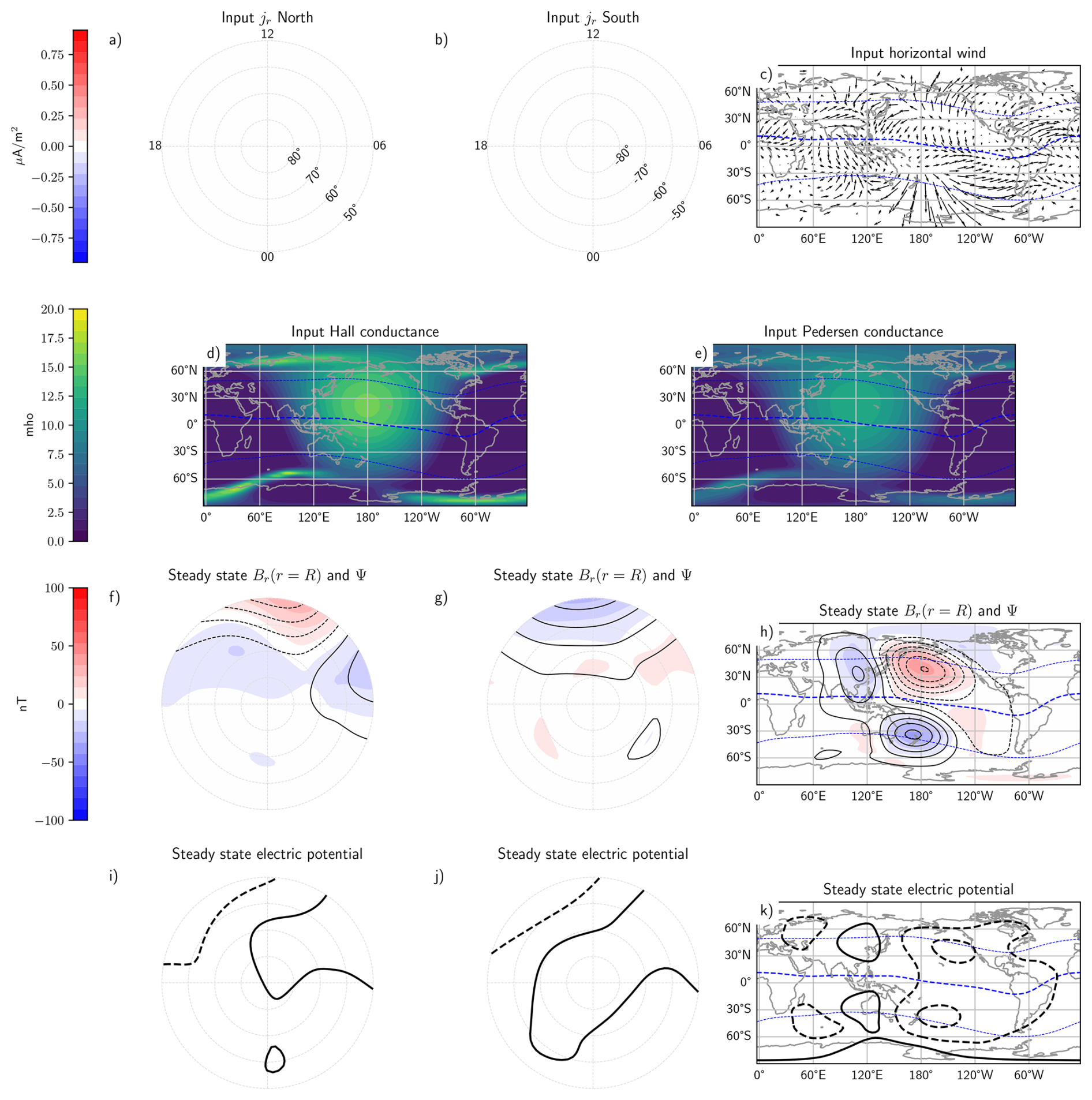
Figure 2 Simulation inputs and steady-state solutions for simulation case 1, where input high-latitude FACs are zero. Polar maps show parameters in Modified Apex latitude and magnetic local time, while global maps are in geographic coordinates with local noon at the center. The input parameters are the field-aligned currents in the Northern (a) and Southern Hemispheres (b); the horizontal winds (c); and the Hall (d) and Pedersen (e) conductance. All input parameters are represented using spherical harmonics, which may differ slightly from their empirical model origins (Drob et al., 2015; Hardy et al., 1987); the spherical harmonic representations shown in the figure are used in our simulations. Based on these inputs, the steady-state solution for the radial magnetic field at r=R is shown in panels (f) (Northern hemisphere), (g) (Southern hemisphere), and (h), with colors representing the field magnitude. Black contours in these panels indicate the equivalent current, spaced at intervals of 20 kA. Panels (i) (Northern hemisphere), (j) (Southern hemisphere), and (k) show the steady-state electric potential, with contours spaced at 3 kV. The induction electric field is zero in the steady state and therefore does not appear in the figure. The blue lines in the global plots represent the magnetic dip equator (dashed) and ±45° Modified Apex latitude, which is the boundary between high and low latitudes used in our simulations.

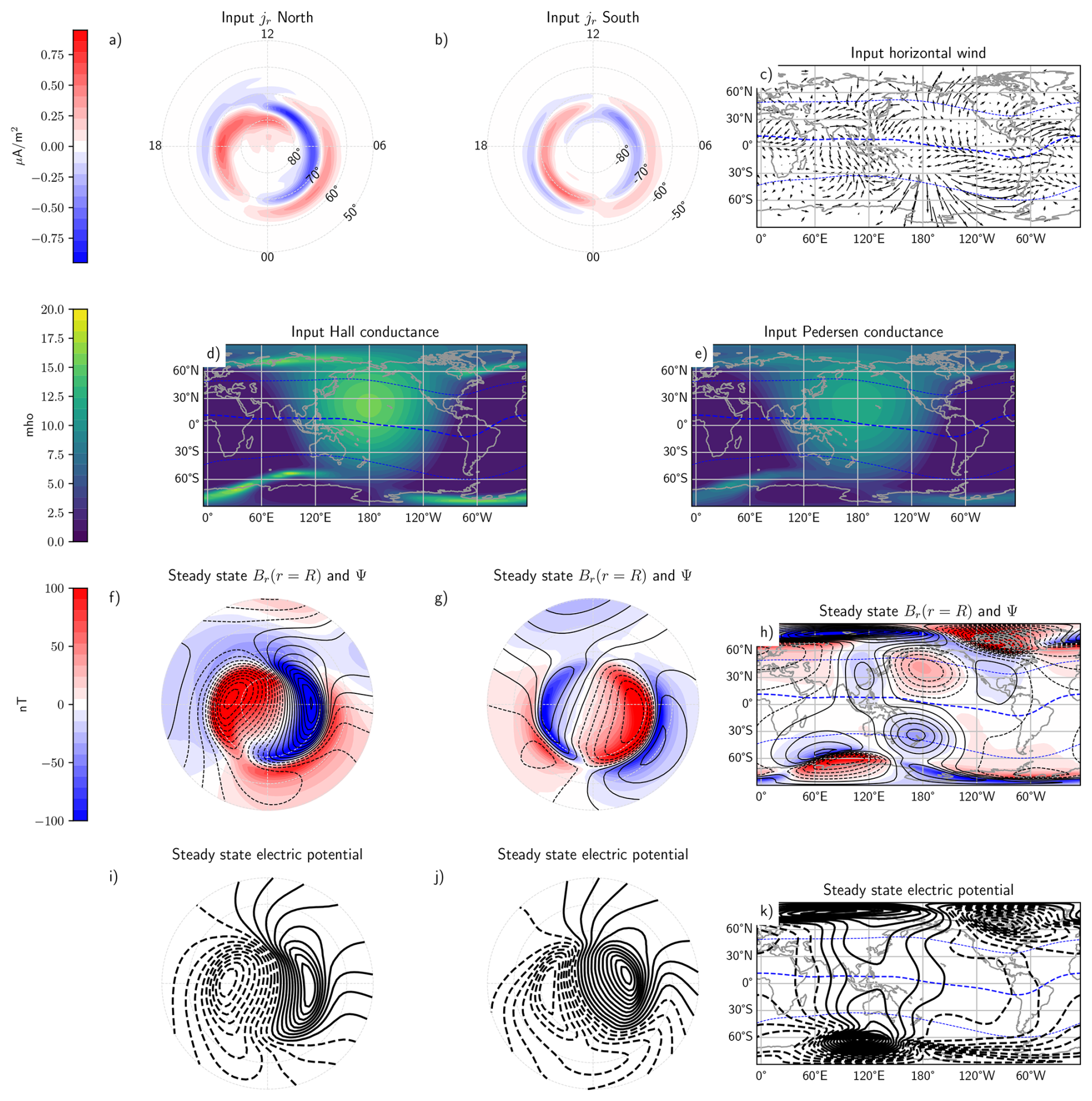
Figure 3 Simulation inputs and steady-state solutions for simulation case 2. The format of the figure is the same as in Fig. 2. The input high-latitude FACs are from the AMPS model (Laundal et al., 2018).

Figures 2 and 3 show the input parameters and corresponding steady-state solutions for the two cases. The two top rows show the input patterns of FACs (a and b), winds (c), and conductance (d and e). The two bottom rows show the steady-state electric potential for this input. We will show below the inductive part of the electric field that is present before steady state is reached. The global maps show the Earth on 1 June 2001, 00:00 UT with local noon at the center. The main magnetic field is given by the International Geomagnetic Reference Field (IGRF) (Alken et al., 2021) for the time of our simulation. The dashed blue lines in the global maps show the dip equator, where b_r=0, and the boundaries between high and low latitudes, set here to 45° Modified Apex latitude (Richmond, 1995). The coordinates in these maps refer to geographic coordinates, while the coordinates in the polar maps refer to Modified Apex latitude and magnetic local time (Laundal and Richmond, 2017). Our simulations are carried out in geocentric spherical coordinates. We truncate the spherical harmonic expansion at $n,m=\mathrm{90}$, corresponding to a spatial resolution of about 400–500 km. The color scales and contour spacing are the same across both Figs. 2 and 3 and throughout the subsequent simulation result figures.

The Hall and Pedersen conductances are given as $\sqrt{{\mathrm{\Sigma }}_{\mathrm{aurora}}^{\mathrm{2}}+{\mathrm{\Sigma }}_{\mathrm{EUV}}^{\mathrm{2}}+{\mathrm{\Sigma }}_{\mathrm{background}}^{\mathrm{2}}}$ on a grid, and then represented with surface spherical harmonics. Σ_aurora is the conductance produced by auroral precipitation, here defined by the precipitation model by Hardy et al. (1987) for Kp=4 converted to conductance using the equations by Robinson et al. (1987). Σ_EUV is the solar EUV-produced conductance, which is based on a simple empirical model by Moen and Brekke (1993) but rigorously accounts for the circular shape of Earth (Laundal et al., 2022b). This model approximately captures the conductance's dependence on plasma density resulting from ionization by solar EUV radiation, but it does not account for the conductance's dependence on magnetic field strength (Richmond, 2016). The main magnetic field varies significantly across the Earth, and the resulting conductance variations may influence the induction process. This effect is not addressed here and may be explored in future work. Σ_background is a constant set to 2 mho in our simulations, that represents a background conductance, sometimes referred to as starlight conductance. The three contributions are combined using quadratic addition due to the mainly quadratic density dependence of the plasma decay in the E-region (Robinson et al., 2021).

The horizontal wind vectors are from the Horizontal Wind Model (HWM) by Drob et al. (2015), evaluated with code by Ilma (2017) at 110 km altitude and with an Ap index of 35. Although vertical winds should ideally be included in our simulation (u_r in Eq. 11), their contribution is minimal outside the equatorial region because of the main field geometry, and since the HWM only provides horizontal winds, we have opted to neglect them in this analysis.

The field-aligned current patterns are given by the Average Magnetic Field and Polar Current System (AMPS) model (Laundal et al., 2018) for a solar wind speed of 400 m s⁻¹, IMF B_y=4 nT, $B_z=-\mathrm{5}$ nT, F_10.7=100 sfu, and a dipole tilt angle calculated to be 18.3° for the time chosen for our simulation.

4.1 Inductive Formation of Sq Currents

Figure 4 shows global maps of the radial magnetic field B_r at r=R and the equivalent current function Ψ (Eq. 23) at different simulation times following a step-function increase at t=0 in winds or conductance (both yielding the same result) to the patterns in Fig. 2c–e. We see that during the seven minutes included here, a mid/low-latitude current pattern develops on the dayside (center of the maps) with a clockwise cell in the Northern hemisphere and an anti-clockwise cell in the Southern hemisphere. This is the Sq current system, which is driven by neutral winds (Yamazaki and Maute, 2017). In this model, the Sq current system results from the magnetic field deformation implied by the induction equation, driven by a static wind pattern and the hemispheric linkage described in Sect. 3.2.1, rather than being derived from electrostatic potentials obtained from solving the current continuity equation as in previous models (Richmond, 2016). Current continuity is always maintained in our simulations since we use Ampère's law without displacement currents (Eq. 10).

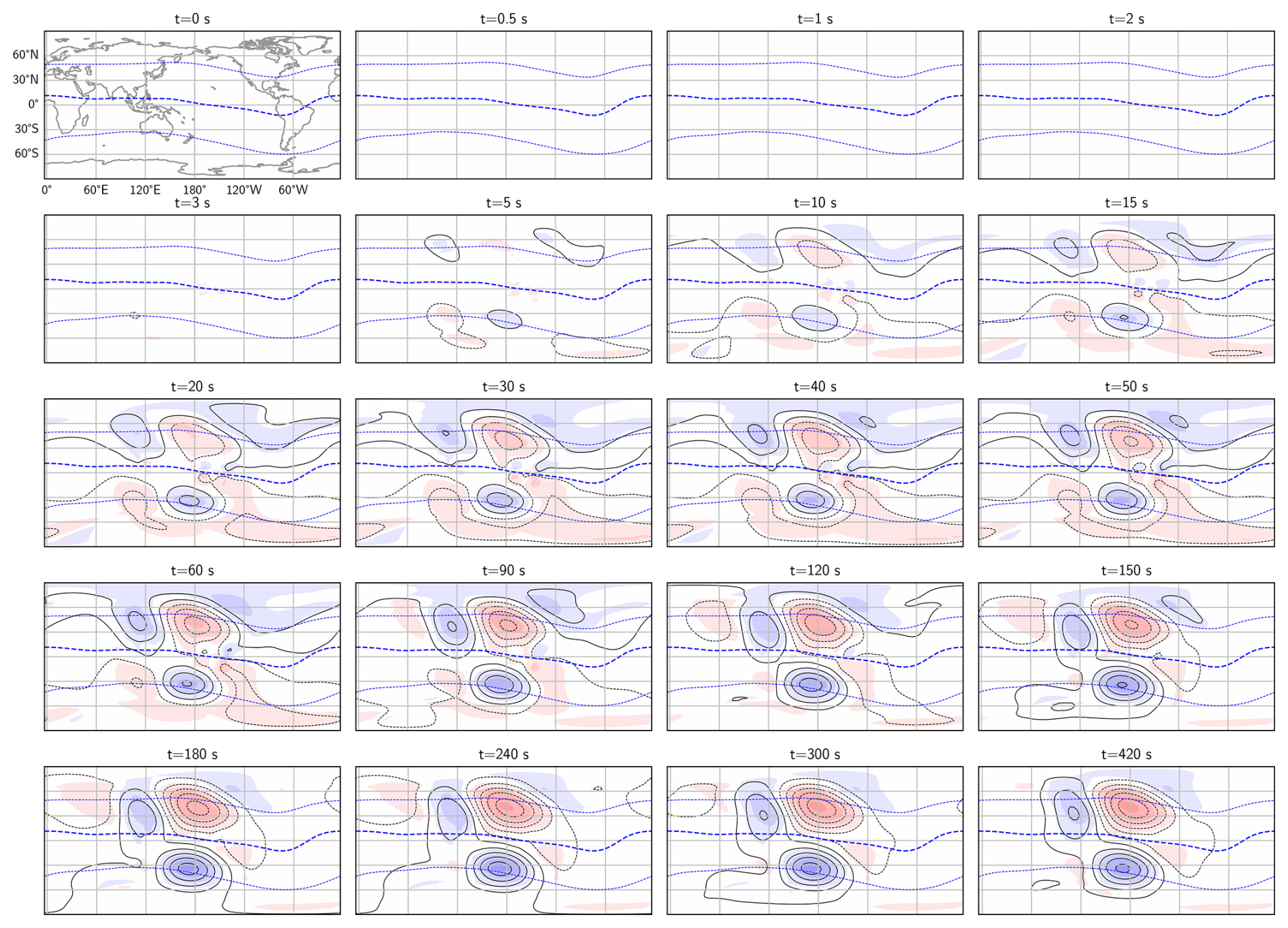
Figure 4 The radial magnetic field (shown in colors) and equivalent current (black contours, spaced at 20 kA intervals) are plotted at 16 different simulation times, following a step increase in winds and/or conductance from zero to the values shown in Fig. 2. The simulation time in seconds is indicated above each panel. The plots are presented in geographic coordinates with noon at the center (consistent with Fig. 2). The blue dashed lines are the magnetic dip equator and contours of ± 45° Modified Apex latitude. The color scale for B_r(r=R) is identical to that in Fig. 2.

Figure 5 shows maps for the same simulation times as in Fig. 4, but this time of the surface electric field (Eq. 7). The surface electric field can be written as

$$\begin{array}{}\text{(38)}& {\mathit{E}}_{\mathrm{S}}=-{\mathrm{\nabla }}_{\mathrm{S}}\mathrm{\Phi }+\widehat{\mathit{r}}\times {\mathrm{\nabla }}_{\mathrm{S}}W,\end{array}$$

where Φ and W are scalar fields. Φ is the electric potential, and its isocontours, spaced by 3 kV, are shown in black in Fig. 5. W is the electric field stream function, and its isocontours, also spaced by 3 kV, are shown in orange. While the contour lines of Φ are perpendicular to the potential electric field, the contours of W are parallel to the rotational part of the electric field. The corresponding plasma flow above the ionosphere, where ideal MHD holds, will be perpendicular to the induction contours, which means that it describes a compression or expansion of the plasma. Only W contributes to $(\mathrm{\nabla }\times \mathit{E})\cdot \widehat{\mathit{r}}$ and therefore only W is directly related to temporal variations in the magnetic field. Even though there are no contour lines of W visible after 50 s, its impact remains visible in the changing Φ and in the changing magnetic field in Fig. 4. The magnitude and scale sizes of the Sq currents in Fig. 4 and low-latitude electric field in Fig. 5 are consistent with typical patterns reported in the literature (e.g., Yamazaki and Maute, 2017, and Richmond et al., 1980).

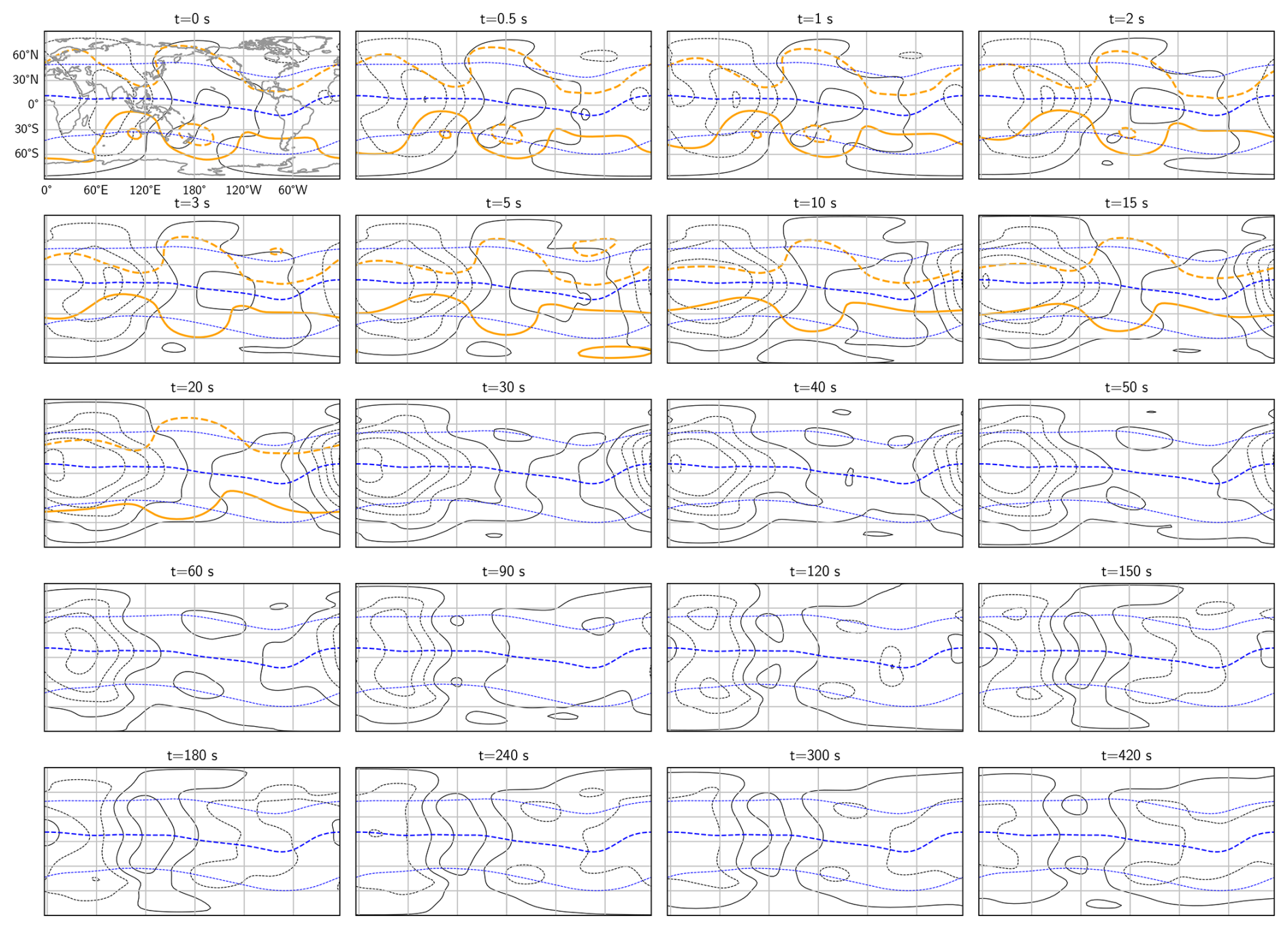
Figure 5 The electric potential Φ (black contours) and electric stream function W (orange contours) at various simulation times, following a step increase in the winds and/or conductance from zero to the values shown in Fig. 2. Φ and W are defined in Eq. (38). The contour spacing is 3 kV for both scalar fields. The simulation times and map projection are the same as in Fig. 4.

4.2 Dynamic Response to FAC Increase

Figures 6–9 show the response in the magnetic and electric fields, respectively, during the seven minutes following a step increase in high-latitude field-aligned currents, from zero to the patterns shown in Fig. 3a and b. The wind and conductance is the same as in the no-FAC case, and the initial condition for this simulation is the steady state solution for the no-FAC case shown in Fig. 2f–k.

Figures 6 and 7 focus on the polar regions and display the response in the magnetic and electric fields, respectively, as functions of magnetic latitude and local time. These figures show that the smaller scale sizes emerge quickly, within few seconds, while the large-scale field continues to change slowly for several tens of seconds. The induction electric field is strong in the beginning, but decreases to a fraction of the potential electric field within about 10 s. It reduces faster in the Southern hemisphere than in the Northern hemisphere because η_P and η_H are higher there due to the lower conductance. We stress that even though the induction electric field quickly becomes small, careful inspection of the last snapshots in Figs. 6 and 7 reveal subtle differences which imply that induction continues to be active for several minutes.

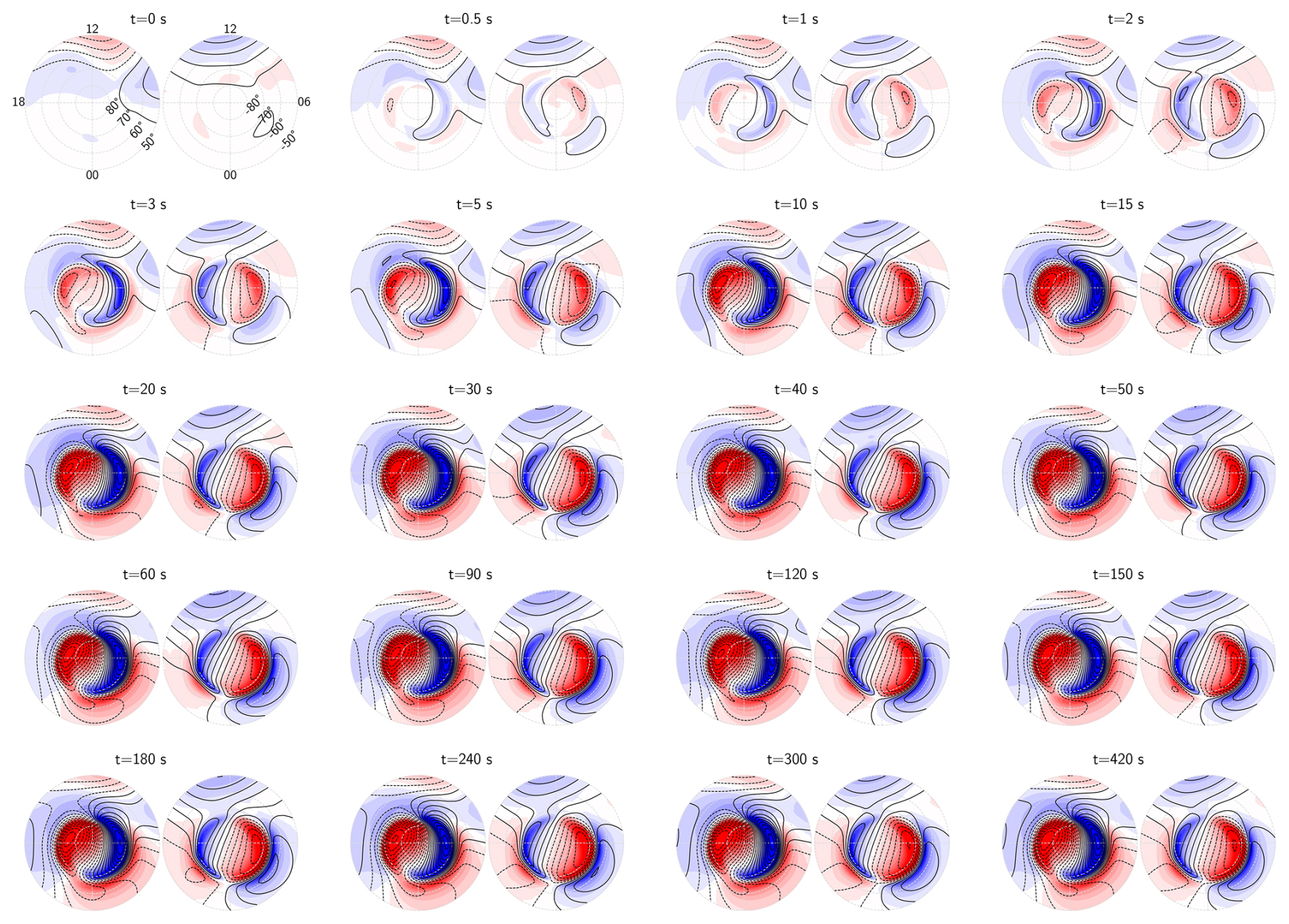
Figure 6 The radial magnetic field (colors) and equivalent current (black contours, spaced at 20 kA intervals) at 16 simulation times, following a step increase in polar field-aligned currents from zero to the values shown in Fig. 3. At each simulation time, a pair of polar plots is displayed, with the northern hemisphere on the left and the southern hemisphere on the right. The initial condition for this simulation is the steady-state solution from Fig. 2 with no FAC but with the same winds and conductance. The simulation time in seconds is indicated above each panel. The plots are presented on Modified Apex latitude and local time grids. The color scale for r=R is identical to that in Figs. 2 and 3.

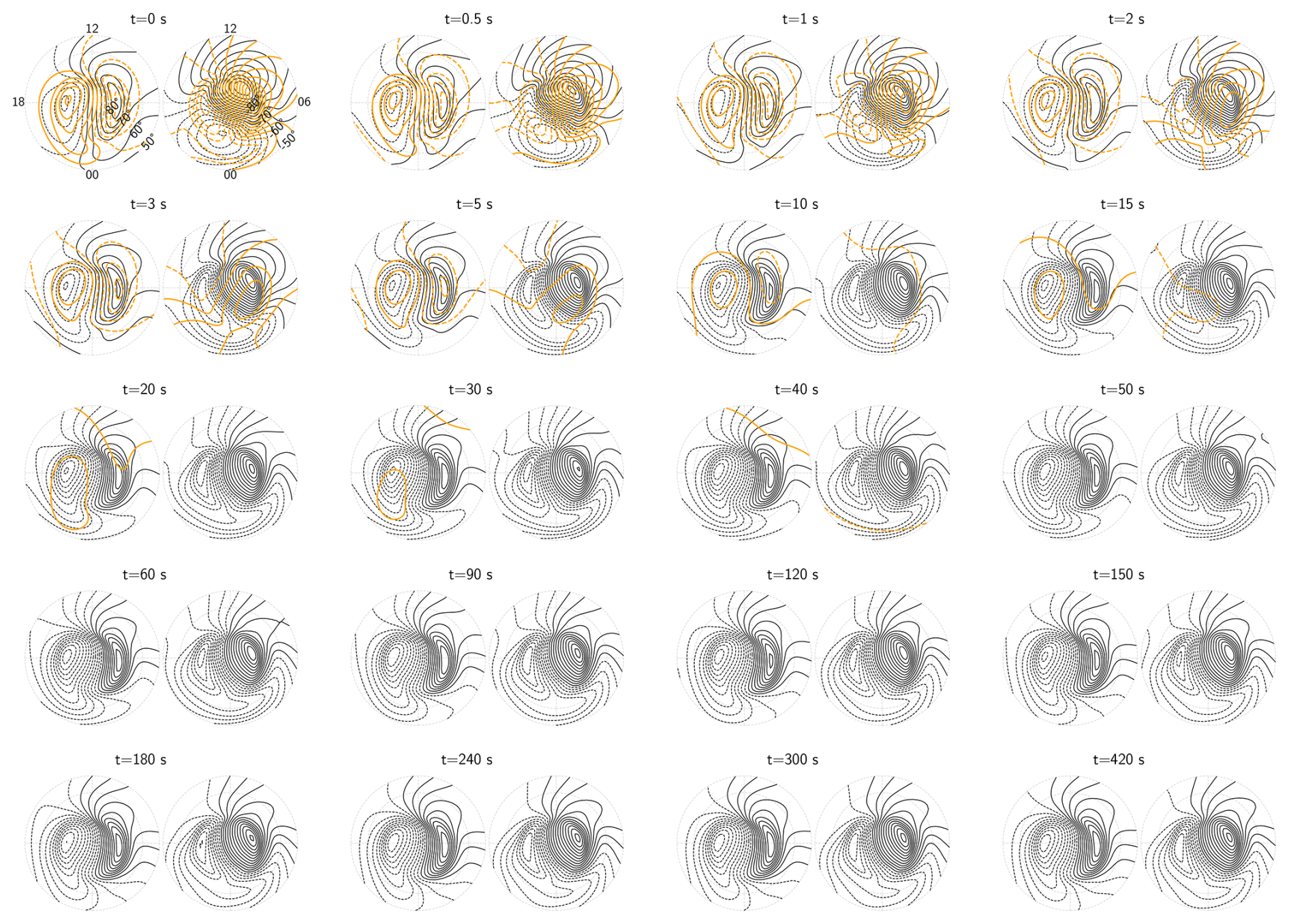
Figure 7 The electric potential (black contours) and electric stream function (orange contours) at various simulation times following a step increase of the high-latitude field-aligned currents from zero to the values shown in Fig. 3. The contour spacing is 3 kV for both scalar fields. The simulation times and map projection are the same as in Fig. 6.

Figures 8 and 9 show the magnetic and electric fields, respectively, on a global scale. In Fig. 8 the first snapshot is identical to Fig. 2h and represents the steady-state solution in the absence of FACs, but with the winds and conductance of Fig. 3c–e. The subsequent snapshots show how B_r and the equivalent current Ψ develop as a result of the step increase in high-latitude FACs. The clearest change is the appearance of the polar currents, the details of which were discussed above. In Fig. 8 we see their equatorward extension, emerging on time scales of several tens of seconds. Another clear change is the emergence of a region with negative B_r (blue) east of the main Sq current cell in the Northern hemisphere, which takes several minutes to develop. This difference in response time at high and low latitudes to a rapid increase in polar FACs is not predicted by conventional models, and might be measurable with for example high time-resolution ground magnetometer networks.

Figure 9 shows the global evolution of the electric field following the step increase in polar FACs. Ten seconds after the increase, we see that a local maximum emerges near midnight (left and right edges of the plots), and continues to increase for 20–30 s, before it decreases and disappears completely after three minutes. This can be interpreted as a transient penetration electric field that corresponds to upward plasma flow in the post-midnight region and downward plasma flow in the pre-midnight region. After seven minutes (the last snapshot) a low-latitude electric field is established that is much stronger and significantly different from the pattern seen in Fig. 5, prior to the increase in high-latitude FACs. The difference can be interpreted as a slowly varying penetration electric field that eventually reaches the steady state shown in Fig. 3k. It is interesting to note that even after seven minutes, we see subtle differences from Fig. 3k, which means that it takes even longer to reach a steady state.

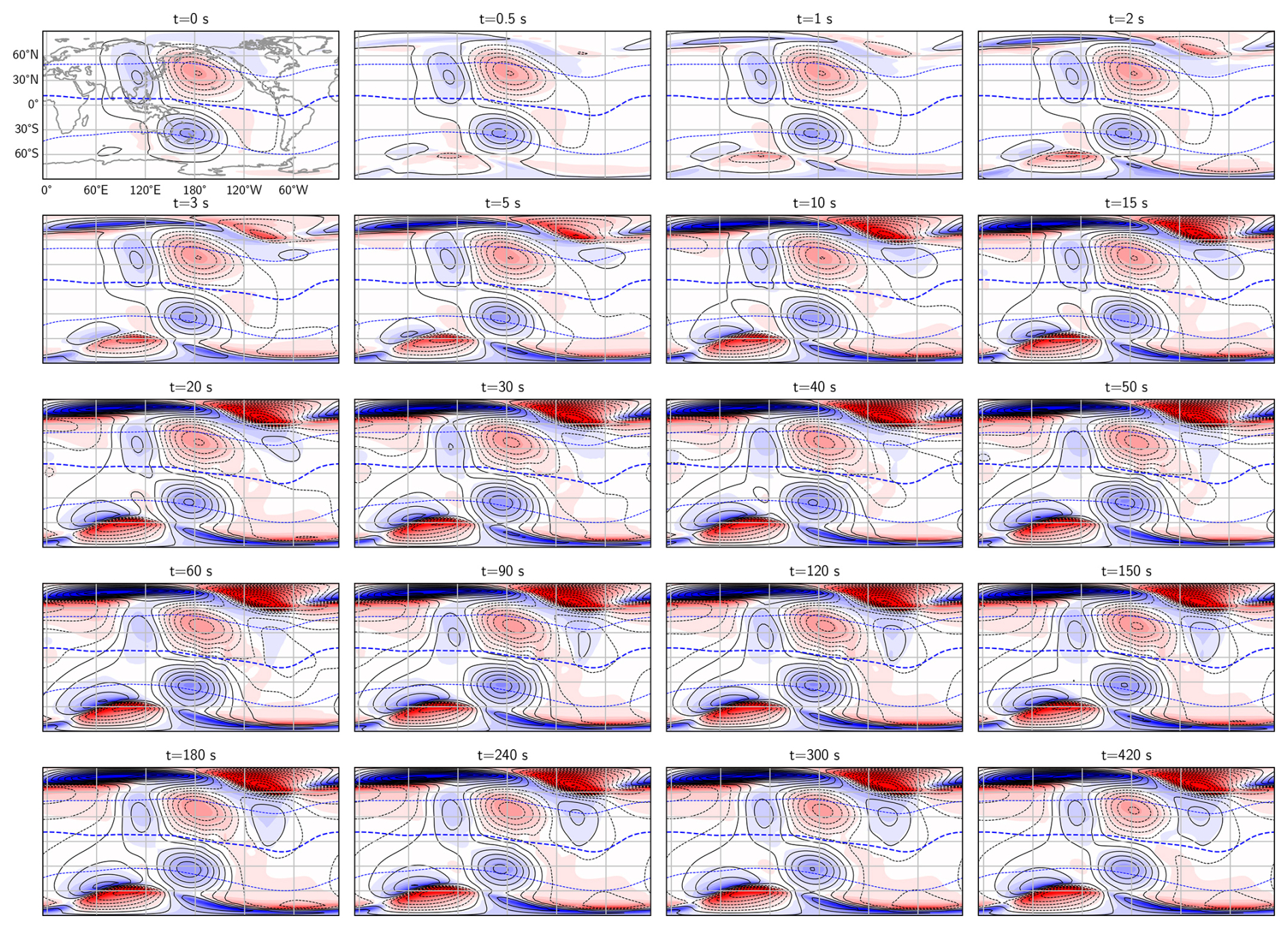
Figure 8 The radial magnetic field and equivalent current from Fig. 6 shown in geographic coordinates. The simulation times, scales, and format are the same as in previous figures.

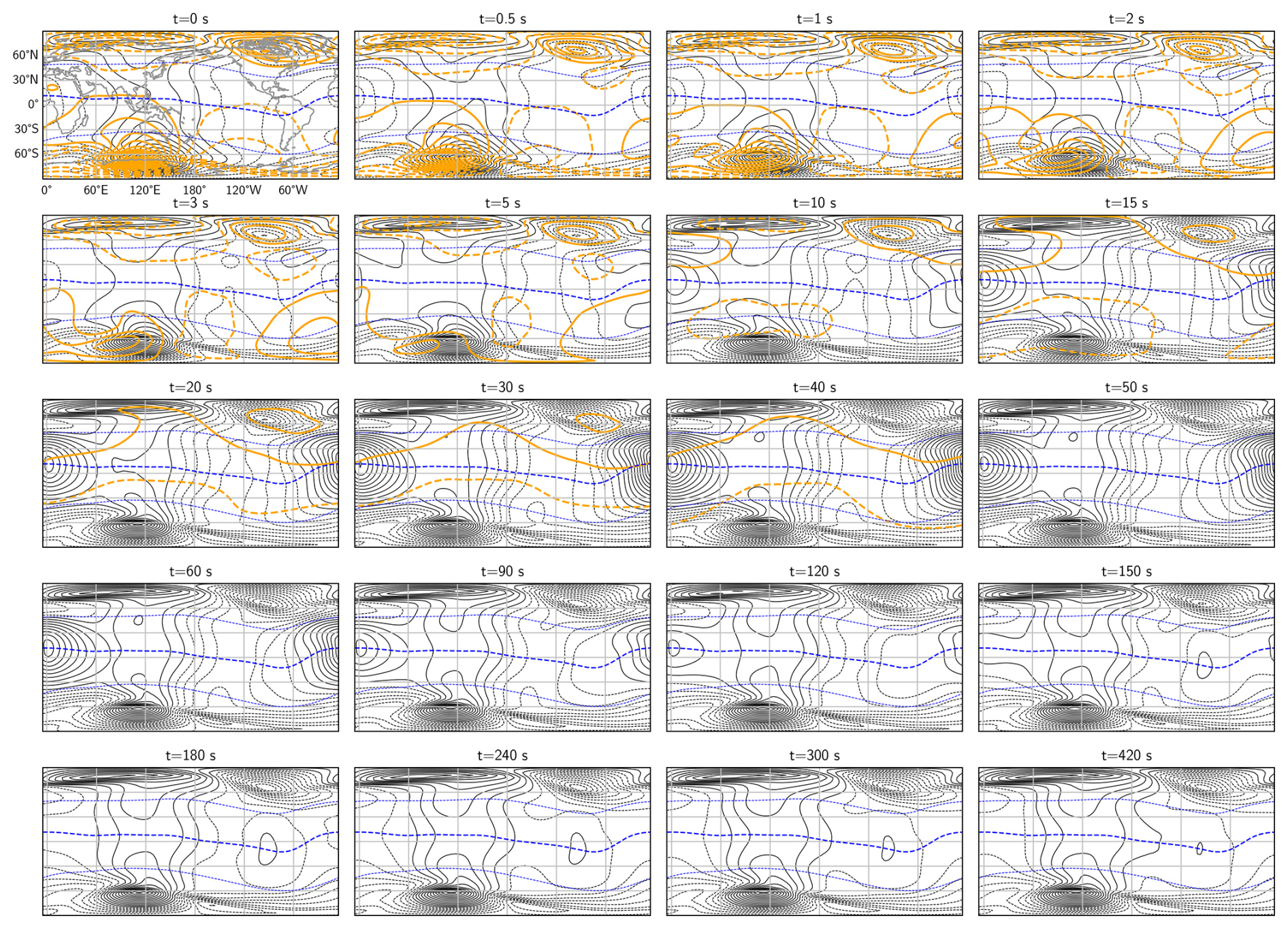
Figure 9 The electric potential and stream function from Fig. 7 shown in geographic coordinates. The simulation times and format are the same as in previous figures.

In the simulations presented here, the FAC, wind, and conductance patterns are held fixed in a geographic coordinate system, instead of slowly rotating them to be fixed with respect to the Sun. The rotation would be slow compared to the time scales of most processes seen in Figs. 4–9, but given that some changes take place over several minutes, induction could nevertheless play a non-negligible role even in the dynamics that results from the rotations of static patterns.

5 Discussion

The model and simulation results presented in this study explain and demonstrate the dynamic interplay between the magnetosphere, ionosphere, and neutral atmosphere. By implementing a global 2D ionospheric model based on the theoretical framework outlined in Sects. 2 and 3, we have demonstrated the effect of induction, as captured by Faraday's law and the Generalized Ohm's law, which combine to Eq. (11). In our model, the electromagnetic fields respond dynamically to changes in the driving parameters – the magnetic field of high-latitude field-aligned currents, neutral winds, or ionospheric conductivity – in contrast to the instant magnetostatic response implied by conventional models for large-scale magnetosphere-ionosphere coupling. While capturing this dynamic response for the first time on a global scale, our model also successfully reproduces key steady-state features of the ionospheric current systems and magnetic field perturbations observed in previous studies, but using a fundamentally different approach. Instead of treating the electric field and current density as the primary variables, as is common in ionospheric physics, the primary parameter of our model is the magnetic field. The velocity could be included as a primary variable by evolving the ion momentum equation in time (Laundal et al., 2024), but for simplicity, we use a steady-state solution here. If needed, the steady-state ion and electron velocities can be calculated using equations from (Brekke, 2013, Chap. 5.1), and the height-integration approach of Laundal et al. (2024). In this way, we offer a framework within the B,v paradigm (Parker, 1996; Vasyliūnas, 2012) to explain the magnetosphere-ionosphere coupling process, capable of accounting for its dynamics.

The simulation results shown in Sect. 4.1 and 4.2 are intentionally idealized, with step changes in winds/conductance and high-latitude field-aligned currents, respectively, to demonstrate the dynamic transition of the ionosphere between states. While these abrupt transitions are artificial, large-scale sudden changes do occur in nature, and our simulations highlight the necessity of accounting for inductive effects when analyzing variations on time scales of tens of seconds. Example of such large-scale rapid changes are solar flares or solar eclipses, which can cause sudden changes in ionospheric conductivity. The inductive effects of these changes have been previously considered (Nagata, 1966), but not with the level of realism achieved by our model. Future work could apply our model with more realistic time profiles of conductance changes associated with solar flares to explore how geomagnetic crochets (e.g., Yamauchi et al., 2020) arise through inductive processes. Another large-scale disturbance where inductive effects should be considered is the sudden increase in solar wind pressure (Madelaire et al., 2022), which propagate through the magnetosphere in seconds and cause magnetic field variations on the ground that imply the presence of significant induction electric fields (Madelaire et al., 2024).

In the rest of this section, we discuss the novel aspects of our model in more detail. Section 5.1 compares our work with previous studies on inductive magnetosphere-ionosphere coupling. Section 5.2 discusses how the perspective on low-latitude wind-driven magnetic field disturbances differs from conventional perspectives. Section 5.3 investigates induction time scales based on an analytical solution to a highly simplified version of the induction equation. Section 5.4 discusses the main limitations of our model and avenues for improvements in future iterations.

5.1 Comparison With Previous Work

Many previous studies of magnetosphere-ionosphere coupling have concentrated on the “gap region” (Merkin and Lyon, 2010), often neglecting the effects of induction at the lower boundary, which is the focus of our investigation. Previous models of magnetosphere-ionosphere coupling typically employ 1D frameworks that consider only the vertical direction (Tu et al., 2011, 2014; Wright, 1996) or 2D models that account for both the vertical dimension and one horizontal dimension (Tu and Song, 2016, 2019; Lotko, 2004; Dreher, 1997; Otto and Zhu, 2003). These studies, many of which also include more detailed treatments of fluid dynamics, have demonstrated that our assumption about the gap region – namely, that the magnetic field rapidly reaches a force-free state – is overly simplistic, particularly on the short time scales we consider. However, all these studies overlook the role of induction at the lower boundary, which we account for in this work. Our results shows the importance of including this lower-boundary induction.

Over the past decades, starting with Yoshikawa and Itonaga (1996), several papers have investigated the inductive response of the ionosphere in terms of Alfvén wave reflection (Buchert and Budnik, 1997), and how it affects ultra-low frequency (ULF) wave propagation (Sciffer et al., 2004; Waters and Sciffer, 2008; Lysak, 2004; Lysak and Song, 2006; Lysak et al., 2020). These studies provide valuable insights into the ionospheric response over different time scales, and clearly demonstrate the need to account for induction in the ionospheric boundary. However, by focusing on wave solutions, they are complicated to use for capturing rapid changes as in the simulations described in Sects. 4.1 and 4.2, or to the magnetosphere-ionosphere coupling schemes required in global magnetospheric simulations. In addition, our approach is arguably more straightforward to expand to capture non-linear behavior.

Vanhamäki (2011) presented an approach for inductive magnetosphere-ionosphere coupling that could overcome these issues. His method shares similarities with ours, using a set of basis functions for the magnetic field to solve for the electric field given the FAC. Instead of spherical harmonics, he used Spherical Elementary Current Systems (SECS) (Amm, 1997; Vanhamäki and Juusola, 2020). The SECS functions are global, but have short reach, which makes them ideal for regional analyses, but less suitable for large-scale domains. Vanhamäki (2011) therefore only demonstrated the technique in a limited region, studying inductive effects in the vicinity of an auroral omega band. In Sect. 5.4.4 we discuss how the approach by Vanhamäki (2011) could be integrated with ours in the future to achieve higher spatial resolution in certain regions.

5.2 Low-latitude Ionospheric Electrodynamics

The global maps in Sect. 4 show that induction processes can play a role for a long time after a step change in winds or FACs, even beyond the seven minutes displayed in the figures.

The slow changes seen at low latitudes can be understood by inspecting the ionospheric induction equation, Eq. (11). The time scale of magnetic field variations (left-hand side) depends on the spatial derivatives and, consequently, the scale sizes of specific combinations of conductance, neutral wind, magnetic field disturbance, and main magnetic field (right-hand side). At low latitudes, the conductance is mainly determined by solar EUV radiation, and gradients are expected to be small. The drivers of the induction at low latitudes are the wind, the poloidal field associated with field-aligned currents, and the corresponding shielding current. Since the field-aligned currents are remote, the structure of this poloidal magnetic field is expected to be dominated by large scales. It may therefore take a long time (tens of seconds to minutes) before the magnetic field of field-aligned currents become visible in low-latitude ground magnetometers.

Our model offers an alternative perspective on low-latitude ionospheric dynamics relative to conventional textbook descriptions. For example, (Kelley, 2009, Chap. 2.6) argues, in response to the B,v-centered view advanced by Vasyliūnas and Song (2005), that “[…]decades of successful application of electroquasistatics in the ionosphere should not be replaced when it is applicable”. While the historical success of electroquasistatics is undisputed in ionospheric physics, our simulations show that important dynamics will be missing without considering how the magnetic field changes through induction. Our results show that even as the system converges toward an electroquasistatic equilibrium, it can take a long time, and involve large-scale intermittent structures in the electric field.

The electroquasistatic approach is computationally efficient, and often yields results that are nearly identical with results from our inductive model that is by comparison more computationally expensive. We nevertheless argue that induction is needed to answer the question of how electric fields and currents change. For example, in our model we see a strong dependence in the low-latitude electric field on the pattern of field-aligned currents at high latitudes. This is the so-called penetration electric field. The term penetration electric field stems from an idea that charges in the inner magnetosphere produces a large-scale electric field (e.g. Kelley, 2009). This contradicts basic facts about space plasmas, since any such charge distribution would quickly (on plasma frequency time scales) be canceled in a frame of reference moving with the plasma (Parker, 2007; Vasyliūnas, 2005, 2012; Parker, 1996). In our model, on the other hand, the electric field is produced in response to a deformation of the magnetic field. The magnetic field deformation changes the Lorentz force, and hence the force balance between the Lorentz force and collisional friction. The ion and electron motion in the ionosphere changes accordingly, and their motion gives the electric field.

In our approach, we assume that the magnetic field deformation related to field-aligned currents occurs instantaneously – an unrealistic simplification – by assuming the magnetic field is perfectly force-free. Simulations by Tu and Song (2019) offer a complementing perspective, resolving plasma dynamics in the vertical dimension and in only a single dimension on the sphere. The propagation of magnetic disturbances from the magnetosphere to the ionosphere as explained by Tu and Song (2019), and the dynamic response of the ionosphere as presented in this paper explains the apparent penetration electric field in terms of B and v. Our simulations also show transient features of the penetration electric field that are impossible to predict with conventional theory, but might be possible to observe in radar measurements.

The traditional explanation of the Sq current system is that neutral winds set up a polarization electric field to ensure charge neutrality, and that this electric field drives currents, and the magnetic field is perturbed accordingly. The inductive formation shown in Sect. 4.1 also starts with the neutral winds, but yields an entirely different description of the chain of causality. The winds do two things: (1) If u×B₀ has a curl, it directly induces a magnetic field perturbation; (2) if u×B₀ at conjugate points imply different electric fields, the magnetic field lines at conjugate points move in different directions and cause magnetic tension to build up. Alfvén waves between hemispheres communicate the imbalance, relaxing the magnetic tension. In reality, this would take some time, but in our study we assume that the balance is reached immediately, and the (imposed) magnetic field adjusts such that the electric potential maps between hemispheres, without violating the assumption of a force-free magnetic field, and current continuity. Sq currents will only form if there is an interhemispheric imbalance in Lorentz force at conjugate points, mainly arising from neutral winds. The formation of the Sq currents is a manifestation of the magnetic field deforming, building up the Lorentz force so that (mainly) ions are pushed through the moving neutral atmosphere while (mainly) electrons act as a neutralizing fluid, moving to preserve charge neutrality. The electric field is determined by this motion. In steady state the electric field is such that no further deformation happens, as the j×B force and momentum transfer due to collisions with neutrals counterbalance each other. At this point, the electric field is purely a potential field, and there is no induction as per Faraday's law.

The critical importance of imbalanced winds at conjugate points agrees with the conclusion by Buchert (2020), who investigated this from an E,j perspective. He describes the low-latitude ionosphere as an entangled dynamo since the winds at conjugate points are coupled.

The equatorial electrojet (EEJ), a narrow channel of intense eastward currents along the dayside dip equator, is missing from the patterns in Sect. 4. This is presumably because the formation of the EEJ involves 3-dimensional structures, as discussed by Yamazaki and Maute (2017), neglected in our 2D approach. In addition, the horizontal resolution of our simulations (≈ 450 km) may anyway be too crude to resolve the EEJ, which extends ≈ 3° to either side of the dip equator (Yamazaki and Maute, 2017).

5.3 Approximating Induction Time Scales With Analytical Solution

It is instructive to consider the highly simplified case of a constant and radial main magnetic field, zero wind, and conductances that are uniform, conditions under which Fukushima's theorem holds (Fukushima, 1976). In that case, we show in Appendix B that Eq. (11) reduces to a differential equation for the coefficients of the induced field $(q_n^m,s_n^m)$, as defined in Eq. (15), as functions of the coefficients of the imposed field (${\mathit{\psi }}_n^m,{\mathit{\xi }}_n^m$). For constant imposed field coefficients, the solution to this equation is

$$\begin{array}{}\text{(39)}& \begin{array}{rl}\left(\begin{array}{c}{q}_n^m\left(t\right)\\ s_n^m\left(t\right)\end{array}\right)=& {\displaystyle \frac{{\mathrm{\Sigma }}_{\mathrm{H}}}{{\mathrm{\Sigma }}_{\mathrm{P}}}}{\displaystyle \frac{n+\mathrm{1}}{\mathrm{2}n+\mathrm{1}}}\left(\begin{array}{c}{\mathit{\psi }}_n^m\\ {\mathit{\xi }}_n^m\end{array}\right)\left[\mathrm{1}-e^{-\frac{{\mathit{\eta }}_{\mathrm{P}}(\mathrm{2}n+\mathrm{1})}{R{\mathit{\mu }}_{\mathrm{0}}}t}\right]\\ & +\left(\begin{array}{c}{q}_n^m(t=\mathrm{0})\\ s_n^m(t=\mathrm{0})\end{array}\right)e^{-\frac{{\mathit{\eta }}_{\mathrm{P}}(\mathrm{2}n+\mathrm{1})}{R{\mathit{\mu }}_{\mathrm{0}}}t}.\end{array}\end{array}$$

In this simplified case, there is no coupling between scale sizes. The exponents show that the characteristic time scales of magnetic field variations depend on scale size (spherical harmonic degree n), the Pedersen resistance η_P, and the radius of the ionosphere R. Figure 10 shows contours of constant e-folding time for different n and Σ_P, with Σ_H held fixed at 5 mho. We see that variations are quickest when Σ_P=Σ_H, ranging from about one min for global scale sizes, to 1 s for n∼ 80–90, which corresponds to scale sizes of about 500 km. We stress that realistic conditions can yield very different results, as illustrated in the previous section.

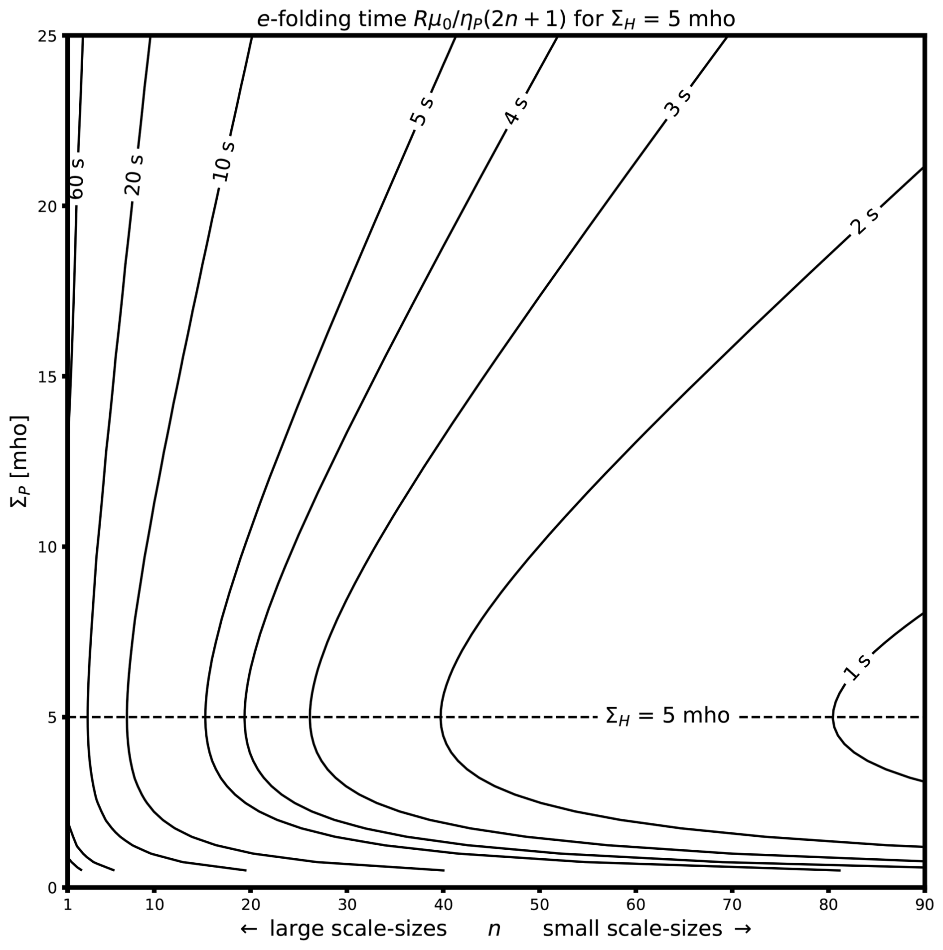
Figure 10 Characteristic time of magnetic field variations at different scale sizes for different Pedersen resistances. In this plot, the Pedersen resistance is varied by setting the Hall conductance to 5 mho and varying the Pedersen conductance.

5.4 Limitations and Potential Enhancements

While the model presented here clearly has limitations, the approach opens several opportunities to study aspects of magnetosphere-ionosphere-thermosphere coupling that have so far not been possible. Here we discuss some of the limitations and how they could be eliminated in future iterations.

5.4.1 From 2D to 3D

Our model is two-dimensional and therefore by definition does not capture dynamics in the vertical direction, including inherently 3D phenomena such as the EEJ. The spherical harmonic representations used here may be difficult to generalize to a 3D ionosphere. An alternative approach could be to use a finite difference or finite volume approach inside a 3D ionosphere, and use our spherical harmonic approach to specify upper and lower boundary conditions. We note that excellent 3D models of the ionosphere already exist (Qian et al., 2014; Huba et al., 2008; Zettergren and Snively, 2015; Ridley et al., 2006), but none of them include induction.

5.4.2 Coupling With Global Magnetosphere Simulations

Our model uses as input the patterns of high-latitude FACs, 2D horizontal wind, and ionospheric conductance, and can output the electric field. These input and output types are also used in magnetosphere-ionosphere coupling modules of global magnetospheric simulations (Merkin and Lyon, 2010; Ridley et al., 2004; Ganse et al., 2025), suggesting that these modules could be replaced with ones based on the approach presented here. This would allow us to study the impact of the magnetosphere on ionospheric induction, and the impact of ionospheric induction on the global magnetosphere.

Our global solver also addresses an inconsistency that can arise in existing models: In conventional approaches, the current continuity equation is solved independently for the electric potential in each hemisphere. This approach does not guarantee consistent mapping of the potential between conjugate points, violating the assumptions of ideal MHD in the magnetosphere and no induction in the ionosphere (Hesse et al., 1997). In contrast, our approach includes induction in the ionosphere, which means that an electric potential mismatch between hemispheres is not in violation of the assumptions of the model. In addition, in our approach, the ionosphere behaves more like a dynamic fluid cell at the inner edge of the magnetosphere rather than a rigid boundary. As a result, abrupt changes in ionospheric conductance, neutral winds, or high-latitude magnetic field perturbations (or field-aligned currents) do not produce the same sudden, potentially unphysical changes in the ionospheric electric field seen in conventional magnetostatic MI coupling schemes. Instead, the electric field evolves smoothly through induction, reflecting the motion of magnetic field lines. This motion may be asymmetric between hemispheres, influencing the displacement field as described by Laundal et al. (2022a). Although including induction does not ensure that the potential maps along magnetic field lines, as noted by Hesse et al. (1997), the total electric field will map in regions where ideal MHD holds.

5.4.3 Inclusion of Fluid Equations

In this paper we only evolve B_r in time, while the wind, conductance, and high-latitude FACs are given. Evolving the FACs would amount to running a global magnetosphere simulation in parallel, as discussed above. The winds and conductance, however, have their own dynamics in the ionosphere, which we neglect here for simplicity. The conductance depends mainly on the plasma density, which is described by the continuity equation; but it also depends on the collision frequencies which depend on temperature (Schunk and Nagy, 2009), which is described by the energy equation. Including plasma fluid moments in the simulation, as in the 1D simulation presented by Laundal et al. (2024), is likely to reveal more complex dynamics. For example, frictional heating, caused by differential motion between ions and neutrals, raises the temperature. This increase alters collision frequencies and conductances, which, in turn, affect the induction process. The modified induction process further influences frictional heating, creating a nonlinear feedback loop. These complex interactions will be explored in future studies.

5.4.4 Refinement

Our use of spherical harmonics is well suited for global analyses. However, this method becomes increasingly ineffective with increasing spatial resolution due to the rapidly growing number of terms required in the spherical harmonic expansion. To address this, our model could be improved by combining spherical harmonics with Spherical Elementary Current Systems (SECS). In this hybrid approach, spherical harmonics would provide the background global representation, while SECS could be used to superimpose a high-resolution magnetic field on a fine grid in specific regions of interest. To implement this consistently and account for the poloidal magnetic field of field-aligned currents, the standard SECS functions would need to be modified. Specifically, the poloidal field of the field-aligned currents must be incorporated along realistic magnetic field geometries, following an approach similar to Vanhamäki et al. (2020) using dipole field lines.

5.4.5 Inclusion of Telluric Currents

In this paper we have neglected the conductivity of the Earth. In reality, the magnetic field induced in the ionosphere leads to currents flowing in the interior of the Earth. Accounting for these induced currents is important for the interpretation of ground magnetometer data, since ground magnetometers observe a combination of ionospheric and telluric magnetic fields. While this issue has been discussed extensively in the literature (e.g., Juusola et al., 2016, 2020; Olsen et al., 2010), the influence of ground induction on ionospheric dynamics is much less studied. Vanhamäki et al. (2005) made simple order-of-magnitude estimates of this effect by using 1D ground conductivity and complex image method with realistic ionospheric sources, and concluded that the effect of ground induction on ionospheric dynamics is significantly smaller than the effect of ionospheric self-induction. However, recently Juusola et al. (2024) made more detailed calculations with 3D ground conductivity and showed that telluric induction can significantly modify the inductive electric field in the ionosphere and should not be ignored.

Including ground induction in our model would change the lower boundary condition for the ionosphere, B⁻. To account for ground induction, the Laplace equation must be solved for the potential magnetic field below the ionosphere V^e with more accurate lower boundary conditions. With spherical harmonics, this can be done with transfer functions that depend on ground conductivity, and map between the ionospheric magnetic field observable from the ground (described here by coefficients $k_n^m$ and $l_n^m$) and spherical harmonic coefficients that describe the induced magnetic field in the ground (e.g., Grayver et al., 2021). While this is feasible, it is beyond the scope of this paper.

6 Conclusions

We have presented a new model to describe magnetosphere-ionosphere-thermosphere coupling on a global scale, that takes into account the induction equation, Faraday's law. Our approach treats the magnetic field as the primary variable, while currents and electric fields are evaluated from Ampère's law and the Generalized Ohm's law, respectively. In this way, our work deviates from the E,j-centered view that is conventionally taken in ionospheric physics, but aligns with how space plasmas are handled elsewhere (Leake et al., 2014; Parker, 2007).

Results from numerical simulations, using spherical harmonic representations of the various quantities (see Sect. C), were presented in Sect. 4. The results show that induction takes place on a broad range of time scales, from fractions of seconds to minutes. The time scale depends on the magnitudes and spatial scales of conductances, imposed magnetic field, neutral wind, and on the main magnetic field geometry (Eq. 11). Large-scale structures at low latitudes take particularly long to adapt to sudden changes in polar FACs, winds, or conductance.

Our model is two-dimensional, and uses as boundary condition an imposed magnetic field that is in reality a result of an inductive process above the ionosphere that we neglect here for simplicity. At high latitudes, the imposed magnetic field is defined to be consistent with a prescribed pattern of field-aligned currents; at low latitudes it is calculated by assuming that the magnetic field adapts to preserve current continuity between hemispheres and matching electric potentials along magnetic field lines, given a neutral wind pattern. These assumptions lead to Sq currents and low-latitude electric fields appearing through induction in our simulations, representing, to our knowledge, the first time that this has been demonstrated.

The model presented here can in principle be incorporated into global magnetosphere simulations and upper-atmospheric circulation models to provide a more complete description of magnetosphere–ionosphere interactions. Steady-state solutions for the electric field can also be obtained, see Sect. C for implementation details. This gives a truly global alternative to prevailing magnetostatic models, which invoke boundary conditions that decouple high and low latitudes. The numerical implementation of the model, used to produce the simulation results presented here, is discussed in Sect. C.

Appendix A: Derivation of the Thin-Sheet Conductivity and Resistivity Tensors

In Sect. 3 we present a two-dimensional version of the Generalized Ohm's law for a collisional ionosphere (Eq. 7). The equation is a projection of the corresponding 3D Eq. (3) onto a spherical shell and so it is valid for an ionosphere that is truly two-dimensional. Nevertheless, as indicated by the choice of notation, we interpret J_S and Σ_P,H as the height-integrated versions of the corresponding 3D quantities j and σ_P,H. If j or σ_P,H vary with height, which they do in the realistic ionosphere, Eq. (7) is not simply a height integral of Eq. (2), so this interpretation requires more justification.

The justification is provided by using the ionospheric Ohm's law, and then solve this equation for E_S. In the dynamo region of the ionosphere (primarily the E-region), E and B vary only slowly with altitude, whereas the conductivities vary sharply. Because of this scale separation, the altitude dependence is carried almost entirely by the conductivities, so integrating the ionospheric Ohm’s law yields well-defined conductances. For generality we retain a finite field-aligned conductivity σ_∥ (though elsewhere in the paper we assume it to be infinite), and write the ionospheric Ohm's law as

$$\begin{array}{}\text{(A1)}& \mathit{j}={\mathit{\sigma }}_{\mathrm{P}}{\mathit{E}}_{⟂}^{\prime }+{\mathit{\sigma }}_{\mathrm{H}}\widehat{\mathit{b}}\times {\mathit{E}}^{\prime }+{\mathit{\sigma }}_{\parallel }{E}_{\parallel }\widehat{\mathit{b}}.\end{array}$$

Here, ${\mathit{E}}^{\prime }=\mathit{E}+\mathit{u}\times \mathit{B}$ is the electric field in the neutral frame of reference. If we assume that both B (which is dominated by the main field, B₀) and E vary little over the height of the ionosphere, we can integrate this equation to get a 3D height-integrated current:

$$\begin{array}{}\text{(A2)}& \mathit{J}={\mathrm{\Sigma }}_{\mathrm{P}}{\mathit{E}}_{⟂}+{\mathrm{\Sigma }}_{\mathrm{H}}\widehat{\mathit{b}}\times \mathit{E}+{\mathrm{\Sigma }}_{\parallel }{E}_{\parallel }\widehat{\mathit{b}}+\mathit{Q}.\end{array}$$

Here, ${\mathrm{\Sigma }}_{\mathrm{P},\mathrm{H},\parallel }$ are the height-integrated ${\mathit{\sigma }}_{\mathrm{P},\mathrm{H},\parallel }$, and $\mathit{Q}={\mathit{Q}}_{\mathrm{P}}+{\mathit{Q}}_{\mathrm{H}}$, where

$$\begin{array}{}\text{(A3)}& {\displaystyle }{\mathit{Q}}_{\mathrm{P}}& {\displaystyle }=\int {\mathit{\sigma }}_{\mathrm{P}}\left(r\right)\left(\mathit{u}\right(r)\times \mathit{B})\mathrm{d}r\text{(A4)}& {\displaystyle }{\mathit{Q}}_{\mathrm{H}}& {\displaystyle }=\int {\mathit{\sigma }}_{\mathrm{H}}\left(r\right)\left(\mathit{u}\right(r)\times \mathit{B})\times \widehat{\mathit{b}}\mathrm{d}r\end{array}$$

are integrated wind terms weighted by the Pedersen and Hall conductivities (Richmond, 1995; Hatch et al., 2024).

We use that ${\mathit{E}}_{⟂}=\mathit{E}-E_{\parallel }\widehat{\mathit{b}}$ and decompose J in radial (subscript r) and tangential/surface components (subscript S):

$$\begin{array}{}\text{(A5)}& \left(\begin{array}{c}{J}_r\\ {\mathit{J}}_{\mathrm{S}}\end{array}\right)=\left(\begin{array}{c}{\mathrm{\Sigma }}_{\mathrm{P}}{E}_r+{\mathrm{\Sigma }}_{\mathrm{H}}{\left(\widehat{\mathit{b}}\times \mathit{E}\right)}_r+\left({\mathrm{\Sigma }}_{\parallel }-{\mathrm{\Sigma }}_{\mathrm{P}}\right)E_{\parallel }{b}_r+Q_r\\ {\mathrm{\Sigma }}_{\mathrm{P}}{\mathit{E}}_{\mathrm{S}}+{\mathrm{\Sigma }}_{\mathrm{H}}{\left(\widehat{\mathit{b}}\times \mathit{E}\right)}_{\mathrm{S}}+\left({\mathrm{\Sigma }}_{\parallel }-{\mathrm{\Sigma }}_{\mathrm{P}}\right)E_{\parallel }{\widehat{\mathit{b}}}_{\mathrm{S}}+{\mathit{Q}}_{\mathrm{S}}\end{array}\right).\end{array}$$

In our 2D/thin-sheet formulation the discontinuity of the horizontal magnetic field across the ionosphere is described by the Ampère jump condition (Eq. 10). This relation requires a surface current confined to the sheet: J_S in the equation above. Because the discontinuity only involves the horizontal magnetic field above and below, there can be no independent horizontal perturbation field inside the sheet itself. Consequently the sheet current is purely tangential: J_r=0. The horizontal divergence of J_S is in general nonzero and is balanced by the radial current carried in the field-aligned system above. We therefore impose J_r=0 in the radial component of (Eq. A5) and solve for E_r:

$$\begin{array}{}\text{(A6)}& E_r=-{\displaystyle \frac{{\mathrm{\Sigma }}_{\mathrm{H}}{\left(\widehat{\mathit{b}}\times \mathit{E}\right)}_r+\left({\mathrm{\Sigma }}_{\parallel }-{\mathrm{\Sigma }}_{\mathrm{P}}\right)b_r\left({\widehat{\mathit{b}}}_{\mathrm{S}}\cdot {\mathit{E}}_{\mathrm{S}}\right)+Q_r}{{\mathrm{\Sigma }}_{\mathrm{P}}\left(b_{\mathit{\theta }}^{\mathrm{2}}+b_{\mathit{\varphi }}^{\mathrm{2}}\right)+{\mathrm{\Sigma }}_{\parallel }{b}_r^{\mathrm{2}}}}\end{array}$$

This can be inserted in the expression for J_S to get an equation for the surface current that only depends on the horizontal components of the electric field. This is a version of the height-integrated ionospheric Ohm's law that explicitly states the dependence on the conductance and main magnetic field geometry through the tensor ${\mathbb{A}}_{\mathrm{cond}}(\mathrm{\Sigma },\widehat{\mathit{b}})$:

$$\begin{array}{}\text{(A7)}& {\mathit{J}}_{\mathrm{S}}={\mathbb{A}}_{\mathrm{cond}}(\mathrm{\Sigma },\widehat{\mathit{b}}){\mathit{E}}_{\mathrm{S}}+{\mathit{Q}}_{\mathrm{eff}},\end{array}$$

where

$$\begin{array}{}\text{(A8)}& {\mathit{Q}}_{\mathrm{eff}}={\mathit{Q}}_{\mathrm{S}}-{\displaystyle \frac{\left({\mathrm{\Sigma }}_{\parallel }-{\mathrm{\Sigma }}_{\mathrm{P}}\right)b_r{\mathit{b}}_S{Q}_r-{\mathrm{\Sigma }}_{\mathrm{H}}{\left(\widehat{\mathit{r}}\times \widehat{\mathit{b}}\right)}_S{Q}_r}{{\mathrm{\Sigma }}_{\mathrm{P}}\left(b_{\mathit{\theta }}^{\mathrm{2}}+b_{\mathit{\varphi }}^{\mathrm{2}}\right)+{\mathrm{\Sigma }}_{\parallel }{b}_r^{\mathrm{2}}}}.\end{array}$$

is the effective wind, a combination of the tangential/surface component of the integrated wind terms and the contribution that comes from substituting E_r in the surface component. The conductance tensor can be expressed as

$$\begin{array}{}\text{(A9)}& {\mathbb{A}}_{\mathrm{cond}}(\mathrm{\Sigma },\widehat{\mathit{b}})={\displaystyle \frac{\mathrm{1}}{\mathrm{\Delta }}}\left(\begin{array}{cc}K{b}_{\mathit{\varphi }}^{\mathrm{2}}+M(\mathrm{1}-b_{\mathit{\varphi }}^{\mathrm{2}})& (M-K)b_{\mathit{\theta }}{b}_{\mathit{\varphi }}-{\mathrm{\Sigma }}_{\mathrm{H}}{\mathrm{\Sigma }}_{\parallel }{b}_r\\ (M-K)b_{\mathit{\theta }}{b}_{\mathit{\varphi }}+{\mathrm{\Sigma }}_{\mathrm{H}}{\mathrm{\Sigma }}_{\parallel }{b}_r& K{b}_{\mathit{\theta }}^{\mathrm{2}}+M(\mathrm{1}-b_{\mathit{\theta }}^{\mathrm{2}})\end{array}\right).\end{array}$$

where

$$\begin{array}{}\text{(A10)}& \begin{array}{rl}& \mathrm{\Delta }\equiv {\mathrm{\Sigma }}_{\mathrm{P}}\left(b_{\mathit{\theta }}^{\mathrm{2}}+b_{\mathit{\varphi }}^{\mathrm{2}}\right)+{\mathrm{\Sigma }}_{\parallel }{b}_r^{\mathrm{2}},\\ & K\equiv {\mathrm{\Sigma }}_{\mathrm{P}}^{\mathrm{2}}+{\mathrm{\Sigma }}_{\mathrm{H}}^{\mathrm{2}},\\ & M\equiv {\mathrm{\Sigma }}_{\mathrm{P}}{\mathrm{\Sigma }}_{\parallel }.\end{array}\end{array}$$

This conductance tensor reduces to the expression given by Amm (1996); Rishbeth and Garriott (1969) for b_ϕ=0.

We can solve Eq. (A7) for E_S to get the corresponding 2D Generalized Ohm's law:

$$\begin{array}{}\text{(A11)}& {\mathit{E}}_{\mathrm{S}}={\mathbb{A}}_{\mathrm{cond}}^{-\mathrm{1}}(\mathrm{\Sigma },\widehat{\mathit{b}})\left({\mathit{J}}_{\mathrm{S}}-{\mathit{Q}}_{\mathrm{eff}}\right)={\mathbb{A}}_{\mathrm{res}}(\mathit{\eta },\widehat{\mathit{b}})\left({\mathit{J}}_{\mathrm{S}}-{\mathit{Q}}_{\mathrm{eff}}\right)\end{array}$$

where the inverse of the conductance tensor is the resistance tensor, ${\mathbb{A}}_{\mathrm{res}}(\mathit{\eta },\widehat{\mathit{b}})$:

$$\begin{array}{}\text{(A12)}& {\mathbb{A}}_{\mathrm{res}}(\mathit{\eta },\widehat{\mathit{b}})=\left(\begin{array}{cc}{\mathit{\eta }}_{\mathrm{P}}+\left({\mathit{\eta }}_{\parallel }-{\mathit{\eta }}_{\mathrm{P}}\right)b_{\mathit{\theta }}^{\mathrm{2}}& \left({\mathit{\eta }}_{\parallel }-{\mathit{\eta }}_{\mathrm{P}}\right)b_{\mathit{\theta }}{b}_{\mathit{\varphi }}+{\mathit{\eta }}_{\mathrm{H}}{b}_r\\ \left({\mathit{\eta }}_{\parallel }-{\mathit{\eta }}_{\mathrm{P}}\right)b_{\mathit{\theta }}{b}_{\mathit{\varphi }}-{\mathit{\eta }}_{\mathrm{H}}{b}_r& {\mathit{\eta }}_{\mathrm{P}}+\left({\mathit{\eta }}_{\parallel }-{\mathit{\eta }}_{\mathrm{P}}\right)b_{\mathit{\varphi }}^{\mathrm{2}}\end{array}\right),\end{array}$$

where η_P and η_H are defined in terms of the conductances as in Eqs. (8) and (9), and ${\mathit{\eta }}_{\parallel }=\mathrm{1}/{\mathrm{\Sigma }}_{\parallel }$. We emphasize that η_P,H are not height-integrated resistances, but quantities derived from the height-integrated conductivities.

The resistance tensor (Eq. A12) is equivalent to the matrix defined in Eq. (11) of O'Sullivan and Downes (2006), which is written in Cartesian coordinates, and it reduces to the matrix in Eq. (11) of this paper in the limit ${\mathit{\eta }}_{\parallel }=\mathrm{0}$. We have thus shown that the expression that we get by simply projecting the 3D Generalized Ohm's law to 2D can also be derived by height-integrating the Ionospheric Ohm's law and solving for E. The advantage of this derivation is that it quantifies the relationship between the 2D and 3D quantities. For example, it provides a consistent way to include altitude-dependent winds in the thin-sheet formulation, by calculating the height integrals in Eqs. (A3) and (A4) to give Q_H and Q_P.

Appendix B: Analytical Solution for Radial Magnetic Field, No wind, and Uniform conductance

In this appendix we derive Eq. (39), the analytical solution discussed in Sect. 5.3. This solution applies under some very restrictive assumptions: The main magnetic field B₀ is radial and constant everywhere, the resistances η_P and η_H are uniform, and there are no neutral winds. Then Faraday's law, Eq. (5) reduces to

$$\begin{array}{}\text{(B1)}& {\displaystyle \frac{\partial B_r}{\partial t}}=-{\mathit{\eta }}_{\mathrm{P}}\left({\mathrm{\nabla }}_{\mathrm{S}}\times {\mathit{J}}_{\mathrm{S}}\right)\cdot \widehat{\mathit{r}}\mp {\mathit{\eta }}_{\mathrm{H}}{\mathrm{\nabla }}_{\mathrm{S}}\times \left({\mathit{J}}_{\mathrm{S}}\times \widehat{\mathit{r}}\right)\end{array}$$

where Eq. (7) was used to replace E_S. The second term is negative when B₀ points downward (as in the Northern hemisphere), and positive when it points upward. In the following we proceed only with the negative sign.

The sheet current can always be written as a sum of divergence-free and curl-free parts. In this case, where the main field is radial, the divergence-free part of the current is equal to the equivalent current (Eq. 22). The curl-free part can be written in terms of a potential α, so that we get

$$\begin{array}{}\text{(B2)}& {\mathit{J}}_{\mathrm{S}}=\widehat{\mathit{r}}\times {\mathrm{\nabla }}_{\mathrm{S}}\mathrm{\Psi }-{\mathrm{\nabla }}_{\mathrm{S}}\mathit{\alpha }.\end{array}$$

where α describes the divergent part of J_S. With this representation of J_S we can write Faraday's law as (e.g., Backus, 1986)

$$\begin{array}{}\text{(B3)}& {\displaystyle \frac{\partial B_r}{\partial t}}=-{\mathit{\eta }}_{\mathrm{P}}{\mathrm{\nabla }}_{\mathrm{S}}^{\mathrm{2}}\mathrm{\Psi }-{\mathit{\eta }}_{\mathrm{H}}{\mathrm{\nabla }}_{\mathrm{S}}^{\mathrm{2}}\mathit{\alpha },\end{array}$$

We can represent α in terms of the spherical harmonic coefficients ${\mathit{\psi }}_n^m$ and ${\mathit{\xi }}_n^m$. The expression for α is (e.g., Laundal et al., 2016)

$$\begin{array}{}\text{(B4)}& \mathit{\alpha }=-{\displaystyle \frac{R}{{\mathit{\mu }}_{\mathrm{0}}}}\sum _{n,m}{P}_n^m\left(\mathit{\theta }\right)\left[{\mathit{\psi }}_n^m\cos \left(m\mathit{\varphi }\right)+{\mathit{\xi }}_n^m\sin \left(m\mathit{\varphi }\right)\right].\end{array}$$

Both Ψ and B_r can be expanded in terms of spherical harmonics with expansion coefficients $q_n^m$ and $s_n^m$, by replacing $k_n^m$ and $l_n^m$ in Eqs. (23) and (21), respectively, using Eq. (19). With these spherical harmonic representations, and the property that ${\mathrm{\nabla }}_{\mathrm{S}}^{\mathrm{2}}=-n(n+\mathrm{1})/R^{\mathrm{2}}$, Eq. (B3) becomes an equation that relates three spherical harmonic series. These series depend on $q_n^m$ and $s_n^m$ (the Ψ term), their time derivatives (the $\partial B_r/\partial t$ term), and on ${\mathit{\psi }}_n^m$ and ${\mathit{\xi }}_n^m$ (the α term). If we match the different terms in these series, we get the following set of differential equations:

$$\begin{array}{}\text{(B5)}& {\displaystyle \frac{\partial }{\partial t}}\left(\begin{array}{c}{q}_n^m\\ s_n^m\end{array}\right)=-{\displaystyle \frac{\mathrm{1}}{R{\mathit{\mu }}_{\mathrm{0}}}}\left(\begin{array}{c}{\mathit{\eta }}_{\mathrm{P}}(\mathrm{2}n+\mathrm{1})q_n^m+{\mathit{\eta }}_{\mathrm{H}}(n+\mathrm{1}){\mathit{\psi }}_n^m\\ {\mathit{\eta }}_{\mathrm{P}}(\mathrm{2}n+\mathrm{1})s_n^m+{\mathit{\eta }}_{\mathrm{H}}(n+\mathrm{1}){\mathit{\xi }}_n^m\end{array}\right).\end{array}$$

For constant ${\mathit{\psi }}_n^m$ and ${\mathit{\xi }}_n^m$ and specified initial conditions, $q_n^m\left(t\right)$ and $s_n^m\left(t\right)$ for time t>0 are given by Eq. (39).

Appendix C: Discretization

The numerical implementation of the model described in this work involves discretization in terms of a combination of spherical harmonics and grid points. Here, we describe how this is done.

C1 Spherical Harmonic Representation of Scalar and Horizontal vector fields

To perform the spherical harmonic decomposition of scalar fields, we use a spherical harmonic transform approach of solving the linear system

$$\begin{array}{}\text{(C1)}& {\mathbb{G}}_s\stackrel{\mathrm{̃}}{\mathit{s}}=\mathit{s},\end{array}$$

where the forward operator 𝔾_s evaluates vectors of spherical harmonic coefficients $\stackrel{\mathrm{̃}}{\mathit{s}}$ at a given set of grid points, giving the grid-resolved data vector s representing the scalar field s.

Similarly, the spherical harmonic decomposition of horizontal vector fields is done by using a spherical harmonic transform approach of solving the linear system

$$\begin{array}{}\text{(C2)}& {\mathbb{G}}_{\mathit{t}}\stackrel{\mathrm{̃}}{\mathit{t}}=\mathit{t}.\end{array}$$

In this case, the field is two-dimensional, and the model vector is resolved into curl-free and divergence-free parts,

$$\begin{array}{}\text{(C3)}& \stackrel{\mathrm{̃}}{\mathit{t}}=\left(\begin{array}{c}{\stackrel{\mathrm{̃}}{\mathit{t}}}_{\mathrm{cf}}\\ {\stackrel{\mathrm{̃}}{\mathit{t}}}_{\mathrm{df}}\end{array}\right),\end{array}$$

and the grid-resolved data vector into θ and ϕ components

$$\begin{array}{}\text{(C4)}& \mathit{t}=\left(\begin{array}{c}{\mathit{t}}_{\mathit{\theta }}\\ {\mathit{t}}_{\mathit{\varphi }}\end{array}\right).\end{array}$$

The forward operator can be expressed as

$$\begin{array}{}\text{(C5)}& {\mathbb{G}}_{\mathit{t}}=\left(\begin{array}{cc}({\mathbb{G}}_{\mathit{t}}{)}_{\mathit{\theta },\mathrm{cf}}& ({\mathbb{G}}_{\mathit{t}}{)}_{\mathit{\theta },\mathrm{df}}\\ ({\mathbb{G}}_{\mathit{t}}{)}_{\mathit{\varphi },\mathrm{cf}}& ({\mathbb{G}}_{\mathit{t}}{)}_{\mathit{\varphi },\mathrm{df}}\end{array}\right).\end{array}$$

𝔾_θ,cf and 𝔾_ϕ,cf give the grid-resolved θ- and ϕ-components, respectively, of (−∇_S) applied to the spherical harmonics used to represent the scalar potential of the curl-free part of the horizontal vector field. Likewise, 𝔾_θ,df and 𝔾_ϕ,df give the grid-resolved θ- and ϕ-components, respectively, of $(\widehat{\mathit{r}}\times {\mathrm{\nabla }}_{\mathrm{S}})$ applied to the spherical harmonics used to represent the scalar potential of the divergence-free part of the horizontal vector field.

Matrices are denoted by blackboard bold. We use 𝔾_X to denote matrices that transform from spherical harmonics to grid points for the quantity X. All other matrices either transform between different spherical harmonic coefficients or between different quantities on the grid. Vectors and matrices associated with spherical harmonics are marked with a tilde, while those associated with grid points are not.

C2 Matrix formulation of Faraday's Law and the Steady-State Condition

From the two-dimensional Faraday's law in Eq. (5), the time derivative of the spherical harmonic coefficients ${\stackrel{\mathrm{̃}}{\mathit{B}}}_{\mathrm{ind}}$ of the induced magnetic field, which corresponds to the radial component of B, can be written as

$$\begin{array}{}\text{(C6)}& {\displaystyle \frac{\partial {\stackrel{\mathrm{̃}}{\mathit{B}}}_{\mathrm{ind}}}{\partial t}}={\stackrel{\mathrm{̃}}{\mathbb{T}}}_{{\mathit{E}}_{\mathrm{S}}\mapsto \partial {\mathit{B}}_{\mathrm{ind}}/\partial t}{\stackrel{\mathrm{̃}}{\mathit{E}}}_{\mathrm{S}}\end{array}$$

where ${\stackrel{\mathrm{̃}}{\mathit{E}}}_{\mathrm{S}}$ is a spherical harmonic representation of the electric field tangential to the ionosphere, and ${\stackrel{\mathrm{̃}}{\mathbb{T}}}_{{\mathit{E}}_{\mathrm{S}}\mapsto \partial {\mathit{B}}_{\mathrm{ind}}/\partial t}$ is the spherical harmonic representation of $(-\widehat{\mathit{r}}\times {\mathrm{\nabla }}_{\mathrm{S}})$. In Sect. C3, we show how ${\stackrel{\mathrm{̃}}{\mathit{E}}}_{\mathrm{S}}$ depends linearly on the spherical harmonic coefficients of the induced magnetic field, ${\stackrel{\mathrm{̃}}{\mathit{B}}}_{\mathrm{ind}}$, the parameter simulated by Eq. (C6), as well as on the input parameters: the horizontal neutral wind, $\stackrel{\mathrm{̃}}{\mathit{u}}$ and the radial component of the field-aligned current density, $\stackrel{\mathrm{̃}}{{\mathit{j}}_r}$. We get

$$\begin{array}{}\text{(C7)}& {\stackrel{\mathrm{̃}}{\mathit{E}}}_{\mathrm{S}}={\stackrel{\mathrm{̃}}{\mathbb{E}}}_{{\mathit{B}}_{\mathrm{ind}}}{\stackrel{\mathrm{̃}}{\mathit{B}}}_{\mathrm{ind}}+{\stackrel{\mathrm{̃}}{\mathbb{E}}}_{\mathit{u}}\stackrel{\mathrm{̃}}{\mathit{u}}+{\stackrel{\mathrm{̃}}{\mathbb{E}}}_{j_r}{\stackrel{\mathrm{̃}}{\mathit{j}}}_r,\end{array}$$

where the matrices ${\stackrel{\mathrm{̃}}{\mathbb{E}}}_{{\mathit{B}}_{\mathrm{ind}}}$, ${\stackrel{\mathrm{̃}}{\mathbb{E}}}_{\mathit{u}}$, and ${\stackrel{\mathrm{̃}}{\mathbb{E}}}_{j_r}$ are given in Eqs. (C34)–(C36). The coefficients for the radial component of the field-aligned current density is a solution of the linear system

$$\begin{array}{}\text{(C8)}& {\mathbb{G}}_{j_r}{\stackrel{\mathrm{̃}}{\mathit{j}}}_r=\left(\begin{array}{c}{\mathit{j}}_r^{\mathrm{hl}}\\ \mathbf{0}\end{array}\right),\end{array}$$

defined in accordance with Eq. (C1). In this equation, the upper block of the vector (superscript “hl”) refers to grid points at high latitudes, while the lower block refers to grid points at low latitudes, where the hemispheres are connected as described in Sect. 3.2.1. The grid values ${\mathit{j}}_r^{\mathrm{hl}}$ are the user-specified input to the simulation, taken from the AMPS model (Laundal et al., 2018) in the simulations presented in this work. The minimum-norm least-squares solution of the linear system is found by calculating

$$\begin{array}{}\text{(C9)}& {\stackrel{\mathrm{̃}}{\mathit{j}}}_r={\mathbb{G}}_{j_r}^{\mathit{†}}\left(\begin{array}{c}{\mathit{j}}_r^{\mathrm{hl}}\\ \mathbf{0}\end{array}\right)\end{array}$$

where ${\mathbb{G}}_{j_r}^{\mathit{†}}$ denotes the Moore-Penrose inverse of of ${\mathbb{G}}_{j_r}$. Similarly, the coefficients for the horizontal neutral winds is a solution of the linear system

$$\begin{array}{}\text{(C10)}& {\mathbb{G}}_{\mathit{u}}\stackrel{\mathrm{̃}}{\mathit{u}}=\mathit{u}\end{array}$$

defined in accordance with Eq. (C2). The grid values u are the user-specified input, taken from the Horizontal Wind Model (Drob et al., 2015) in the simulations presented in this work. The minimum-norm least-squares solution of the linear system is found by calculating

$$\begin{array}{}\text{(C11)}& \stackrel{\mathrm{̃}}{\mathit{u}}={\mathbb{G}}_{\mathit{u}}^{\mathit{†}}\mathit{u},\end{array}$$

where ${\mathbb{G}}_{\mathit{u}}^{\mathit{†}}$ denotes the Moore-Penrose inverse of 𝔾_u.

To obtain final expressions for Faraday's law and the steady-state condition, we note that the surface electric field coefficients can be separated as

$$\begin{array}{}\text{(C12)}& {\stackrel{\mathrm{̃}}{\mathit{E}}}_{\mathrm{S}}=\left(\begin{array}{c}{\stackrel{\mathrm{̃}}{\mathit{E}}}_{\mathrm{cf}}\\ {\stackrel{\mathrm{̃}}{\mathit{E}}}_{\mathrm{df}}\end{array}\right)=\left(\begin{array}{c}({\stackrel{\mathrm{̃}}{\mathbb{E}}}_{{\mathit{B}}_{\mathrm{ind}}}{\stackrel{\mathrm{̃}}{\mathit{B}}}_{\mathrm{ind}}+{\stackrel{\mathrm{̃}}{\mathbb{E}}}_{\mathit{u}}\stackrel{\mathrm{̃}}{\mathit{u}}+{\stackrel{\mathrm{̃}}{\mathbb{E}}}_{j_r}{\stackrel{\mathrm{̃}}{\mathit{j}}}_r{)}_{\mathrm{cf}}\\ ({\stackrel{\mathrm{̃}}{\mathbb{E}}}_{{\mathit{B}}_{\mathrm{ind}}}{\stackrel{\mathrm{̃}}{\mathit{B}}}_{\mathrm{ind}}+{\stackrel{\mathrm{̃}}{\mathbb{E}}}_{\mathit{u}}\stackrel{\mathrm{̃}}{\mathit{u}}+{\stackrel{\mathrm{̃}}{\mathbb{E}}}_{j_r}{\stackrel{\mathrm{̃}}{\mathit{j}}}_r{)}_{\mathrm{df}}\end{array}\right)\end{array}$$

in accordance with Eq. (C2). The curl of the curl-free part is by definition zero, implying that we can express ${\stackrel{\mathrm{̃}}{\mathbb{T}}}_{{\mathit{E}}_{\mathrm{S}}\mapsto \partial {\mathit{B}}_{\mathrm{ind}}/\partial t}$ as

$$\begin{array}{}\text{(C13)}& {\stackrel{\mathrm{̃}}{\mathbb{T}}}_{{\mathit{E}}_{\mathrm{S}}\mapsto \partial {\mathit{B}}_{\mathrm{ind}}/\partial t}=\left(\begin{array}{cc}\mathbf{0}& {\stackrel{\mathrm{̃}}{\mathbb{T}}}_{{\mathit{E}}_{\mathrm{df}}\mapsto \partial {\mathit{B}}_{\mathrm{ind}}/\partial t}\end{array}\right),\end{array}$$

where ${\stackrel{\mathrm{̃}}{\mathbb{T}}}_{{\mathit{E}}_{\mathrm{df}}\mapsto \partial {\mathit{B}}_{\mathrm{ind}}/\partial t}$ is the diagonal matrix given in Table C1, representing the application of $(-\widehat{\mathit{r}}\times {\mathrm{\nabla }}_{\mathrm{S}})$ on the divergence-free part of E_S. Inserting Eqs. (C12) and (C13) into Eq. (C6), we obtain the following matrix formulation of Faraday's law,

$$\begin{array}{}\text{(C14)}& {\displaystyle \frac{\partial {\stackrel{\mathrm{̃}}{\mathit{B}}}_{\mathrm{ind}}}{\partial t}}={\stackrel{\mathrm{̃}}{\mathbb{T}}}_{{\mathit{E}}_{\mathrm{df}}\mapsto \partial {\mathit{B}}_{\mathrm{ind}}/\partial t}({\stackrel{\mathrm{̃}}{\mathbb{E}}}_{{\mathit{B}}_{\mathrm{ind}}}{\stackrel{\mathrm{̃}}{\mathit{B}}}_{\mathrm{ind}}+{\stackrel{\mathrm{̃}}{\mathbb{E}}}_{\mathit{u}}\stackrel{\mathrm{̃}}{\mathit{u}}+{\stackrel{\mathrm{̃}}{\mathbb{E}}}_{j_r}{\stackrel{\mathrm{̃}}{\mathit{j}}}_r{)}_{\mathrm{df}}.\end{array}$$

When simulating the temporal evolution of the induced magnetic field, we perform a discretized integration of Eq. (C14) using Euler's method,

$$\begin{array}{}\text{(C15)}& {\stackrel{\mathrm{̃}}{\mathit{B}}}_{\mathrm{ind},n+\mathrm{1}}\approx {\stackrel{\mathrm{̃}}{\mathit{B}}}_{\mathrm{ind},n}+{\displaystyle \frac{\partial {\stackrel{\mathrm{̃}}{\mathit{B}}}_{\mathrm{ind},n}}{\partial t}}\mathrm{\Delta }t,\end{array}$$

where we use the time step $\mathrm{\Delta }t=\mathrm{5}\times {\mathrm{10}}^{-\mathrm{4}}$ s for all simulations in this work. The error of this method is of the order O(Δt²).

The steady state of the ionosphere is reached when $\frac{\partial {\stackrel{\mathrm{̃}}{\mathit{B}}}_{\mathrm{ind}}}{\partial t}=\mathrm{0}$. Inserting this constraint into Eq. (C14), we obtain

$$\begin{array}{}\text{(C16)}& {\stackrel{\mathrm{̃}}{\mathbb{T}}}_{{\mathit{E}}_{\mathrm{df}}\mapsto \partial {\mathit{B}}_{\mathrm{ind}}/\partial t}{\left({\stackrel{\mathrm{̃}}{\mathbb{E}}}_{{\mathit{B}}_{\mathrm{ind}}}{\stackrel{\mathrm{̃}}{\mathit{B}}}_{\mathrm{ind}}+{\stackrel{\mathrm{̃}}{\mathbb{E}}}_{\mathit{u}}\stackrel{\mathrm{̃}}{\mathit{u}}+{\stackrel{\mathrm{̃}}{\mathbb{E}}}_{j_r}{\stackrel{\mathrm{̃}}{\mathit{j}}}_r\right)}_{\mathrm{df}}=\mathrm{0}.\end{array}$$

Since ${\stackrel{\mathrm{̃}}{\mathbb{T}}}_{{\mathit{E}}_{\mathrm{df}}\mapsto \partial {\mathit{B}}_{\mathrm{ind}}/\partial t}$ is a diagonal and invertible matrix, we can multiply Eq. (C16) from the left by its inverse, giving

$$\begin{array}{}\text{(C17)}& {\left({\stackrel{\mathrm{̃}}{\mathbb{E}}}_{{\mathit{B}}_{\mathrm{ind}}}{\stackrel{\mathrm{̃}}{\mathit{B}}}_{\mathrm{ind}}\right)}_{\mathrm{df}}=-{\left({\stackrel{\mathrm{̃}}{\mathbb{E}}}_{\mathit{u}}\stackrel{\mathrm{̃}}{\mathit{u}}+{\stackrel{\mathrm{̃}}{\mathbb{E}}}_{j_r}{\stackrel{\mathrm{̃}}{\mathit{j}}}_r\right)}_{\mathrm{df}}.\end{array}$$

This linear system can be solved for the steady state ${\stackrel{\mathrm{̃}}{\mathit{B}}}_{\mathrm{ind}}$. Note that it is also possible to solve the equation for $\stackrel{\mathrm{̃}}{\mathit{u}}$ or ${\stackrel{\mathrm{̃}}{\mathit{j}}}_r$ given the other vectors, which could give alternative approaches to determining horizontal neutral winds or field-aligned currents experimentally, assuming that the system is in steady state.

Thus, it is possible to find both time-dependent and steady-state solutions for the model parameters ${\stackrel{\mathrm{̃}}{\mathit{B}}}_{\mathrm{ind}}$ by solving equations involving conductance-dependent matrices ${\stackrel{\mathrm{̃}}{\mathbb{E}}}_{{\mathit{B}}_{\mathrm{ind}}}$, ${\stackrel{\mathrm{̃}}{\mathbb{E}}}_{\mathit{u}}$ and ${\stackrel{\mathrm{̃}}{\mathbb{E}}}_{j_r}$, obtained from Eqs. (C34)–(C36), respectively, and the spherical harmonic coefficient vectors ${\stackrel{\mathrm{̃}}{\mathit{j}}}_r$ and $\stackrel{\mathrm{̃}}{\mathit{u}}$, obtained from Eqs. (C8) and (C10) with grid-resolved input from external models, respectively.

As a side note, Eq. (C14) represents a linear and time-invariant (LTI) system during periods when the conductance, field-aligned current, and neutral wind are constant. In such cases, solutions at any time within the period can be computed using matrix exponentials (Chen, 2014), bypassing numerical integration. This approach could improve simulation efficiency, particularly in scenarios where these quantities vary slowly compared to the timescales of induction, a common assumption in ionospheric modeling.

C3 Matrix Formulation of the Generalized Ohm's Law

Here, we derive an expression for linearly constructing the spherical harmonic coefficients of the horizontal electric field from those of the induced magnetic field, neutral winds, and field-aligned currents, while accounting for boundary conditions through the imposed magnetic field. This expression, presented in Eq. (C33), is derived from the 2D Generalized Ohm's law in Eq. (7), which can be discretized in terms of grid points and spherical harmonics as

$$\begin{array}{}\text{(C18)}& {\mathbb{G}}_{{\mathit{E}}_{\mathrm{S}}}{\stackrel{\mathrm{̃}}{\mathit{E}}}_{\mathrm{S}}={\mathbb{T}}_{{\mathit{J}}_{\mathrm{S}}\mapsto {\mathit{E}}_{\mathrm{S}}}{\mathbb{G}}_{{\mathit{J}}_{\mathrm{S}}}{\stackrel{\mathrm{̃}}{\mathbb{T}}}_{\mathit{B}\mapsto {\mathit{J}}_{\mathrm{S}}}\stackrel{\mathrm{̃}}{\mathit{B}}+{\mathbb{T}}_{\mathit{u}\mapsto {\mathit{E}}_{\mathrm{S}}}{\mathbb{G}}_{\mathit{u}}\stackrel{\mathrm{̃}}{\mathit{u}},\end{array}$$

where $\stackrel{\mathrm{̃}}{\mathit{B}}$, ${\stackrel{\mathrm{̃}}{\mathit{E}}}_{\mathrm{S}}$ and $\stackrel{\mathrm{̃}}{\mathit{u}}$ are vectors containing the spherical harmonic coefficients of the magnetic field, horizontal electric field and horizontal neutral wind, respectively. ${\stackrel{\mathrm{̃}}{\mathbb{T}}}_{\mathit{B}\mapsto {\mathit{J}}_{\mathrm{S}}}$ is the representation of the jump condition ${\mathit{J}}_{\mathrm{S}}=\frac{\mathrm{1}}{{\mathit{\mu }}_{\mathrm{0}}}\widehat{\mathit{r}}\times \mathrm{\Delta }\mathit{B}$ in the basis of the spherical harmonics used for representing B. The evaluation matrices ${\mathbb{G}}_{{\mathit{E}}_{\mathrm{S}}}$, ${\mathbb{G}}_{{\mathit{J}}_{\mathrm{S}}}$ and 𝔾_u evaluate the spherical harmonic expansions of the horizontal electric field, current and neutral wind, respectively, on a common set of grid points in accordance with Eq. (C2). In the simulations presented in this work, we use a cubed-sphere grid with 100×100 grid points in each of the six cubed-sphere blocks. ${\mathbb{T}}_{{\mathit{J}}_{\mathrm{S}}\mapsto {\mathit{E}}_{\mathrm{S}}}={\mathbb{T}}_{{\mathit{J}}_{\mathrm{S}}\mapsto {\mathit{E}}_{\mathrm{S}}}({\mathit{B}}_{\mathrm{0}},{\mathit{\eta }}_{\mathrm{P}},{\mathit{\eta }}_{\mathrm{H}})$ and ${\mathbb{T}}_{\mathit{u}\mapsto {\mathit{E}}_{\mathrm{S}}}={\mathbb{T}}_{\mathit{u}\mapsto {\mathit{E}}_{\mathrm{S}}}\left({\mathit{B}}_{\mathrm{0}}\right)$ represent the current-dependent and neutral wind-dependent terms in the 2D Generalized Ohm's law, respectively, expressed on the same grid points.

We can obtain the minimum-norm least-squares solution for the spherical harmonic coefficients ${\stackrel{\mathrm{̃}}{\mathit{E}}}_{\mathrm{S}}$ by multiplying Eq. (C18) from the left by the Moore-Penrose inverse of ${\mathbb{G}}_{{\mathit{E}}_{\mathrm{S}}}$, denoted by ${\mathbb{G}}_{{\mathit{E}}_{\mathrm{S}}}^{\mathit{†}}$, giving

$$\begin{array}{}\text{(C19)}& \begin{array}{rl}{\stackrel{\mathrm{̃}}{\mathit{E}}}_{\mathrm{S}}=& {\mathbb{G}}_{{\mathit{E}}_{\mathrm{S}}}^{\mathit{†}}{\mathbb{T}}_{{\mathit{J}}_{\mathrm{S}}\mapsto {\mathit{E}}_{\mathrm{S}}}{\mathbb{G}}_{{\mathit{J}}_{\mathrm{S}}}{\stackrel{\mathrm{̃}}{\mathbb{T}}}_{\mathit{B}\mapsto {\mathit{J}}_{\mathrm{S}}}\stackrel{\mathrm{̃}}{\mathit{B}}\\ & +{\mathbb{G}}_{{\mathit{E}}_{\mathrm{S}}}^{\mathit{†}}{\mathbb{T}}_{\mathit{u}\mapsto {\mathit{E}}_{\mathrm{S}}}{\mathbb{G}}_{\mathit{u}}\stackrel{\mathrm{̃}}{\mathit{u}}.\end{array}\end{array}$$

Continuing, we decompose the magnetic field B into the sum of its induced part B_ind and its imposed part B_imp, in accordance with Sect. 3, implying that $\stackrel{\mathrm{̃}}{\mathit{B}}$ can be written as

$$\begin{array}{}\text{(C20)}& \stackrel{\mathrm{̃}}{\mathit{B}}=\left(\begin{array}{c}{\stackrel{\mathrm{̃}}{\mathit{B}}}_{\mathrm{ind}}\\ {\stackrel{\mathrm{̃}}{\mathit{B}}}_{\mathrm{imp}}\end{array}\right).\end{array}$$

Similarly, the matrix evaluating J_S from the model vector $\stackrel{\mathrm{̃}}{\mathit{B}}$ can be separated into blocks referencing the induced and imposed parts of the magnetic field,

$$\begin{array}{}\text{(C21)}& {\stackrel{\mathrm{̃}}{\mathbb{T}}}_{\mathit{B}\mapsto {\mathit{J}}_{\mathrm{S}}}=\left(\begin{array}{cc}{\stackrel{\mathrm{̃}}{\mathbb{T}}}_{{\mathit{B}}_{\mathrm{ind}}\mapsto {\mathit{J}}_{\mathrm{S}}}& {\stackrel{\mathrm{̃}}{\mathbb{T}}}_{{\mathit{B}}_{\mathrm{imp}}\mapsto {\mathit{J}}_{\mathrm{S}}}\end{array}\right).\end{array}$$

where the spherical harmonic transformation matrices ${\stackrel{\mathrm{̃}}{\mathbb{T}}}_{{\mathit{B}}_{\mathrm{ind}}\mapsto {\mathit{J}}_{\mathrm{S}}}$ and ${\stackrel{\mathrm{̃}}{\mathbb{T}}}_{{\mathit{B}}_{\mathrm{imp}}\mapsto {\mathit{J}}_{\mathrm{S}}}$ are given in Table C1. The matrix ${\stackrel{\mathrm{̃}}{\mathbb{T}}}_{{\mathit{B}}_{\mathrm{imp}}\mapsto {\mathit{J}}_{\mathrm{S}}}$ includes the contribution to the poloidal field coming from the toroidal B_imp, representing the Biot-Savart integral of the horizontal part of the field-aligned currents above the ionosphere, as discussed in Sect. 3.2.2. The discretization procedure is discussed in Sect. C4. Inserting Eqs. (C20) and (C21) into Eq. (C19), we obtain

$$\begin{array}{}\text{(C22)}& \begin{array}{rl}{\stackrel{\mathrm{̃}}{\mathit{E}}}_{\mathrm{S}}=& {\stackrel{\mathrm{̃}}{\mathbb{T}}}_{{\mathit{B}}_{\mathrm{ind}}\mapsto {\mathit{E}}_{\mathrm{S}}}{\stackrel{\mathrm{̃}}{\mathit{B}}}_{\mathrm{ind}}+{\stackrel{\mathrm{̃}}{\mathbb{T}}}_{{\mathit{B}}_{\mathrm{imp}}\mapsto {\mathit{E}}_{\mathrm{S}}}{\stackrel{\mathrm{̃}}{\mathit{B}}}_{\mathrm{imp}}\\ & +{\stackrel{\mathrm{̃}}{\mathbb{T}}}_{\mathit{u}\mapsto {\mathit{E}}_{\mathrm{S}}}\stackrel{\mathrm{̃}}{\mathit{u}},\end{array}\end{array}$$

where the spherical harmonic coefficient transformation matrices ${\stackrel{\mathrm{̃}}{\mathbb{T}}}_{X\mapsto {\mathit{E}}_{\mathrm{S}}}$ are given in Table C1

${\stackrel{\mathrm{̃}}{\mathit{B}}}_{\mathrm{imp}}$ depends on the specified field-aligned currents at high latitudes and on the constraints that the current density and electric field map between hemispheres at low latitudes, as discussed in Sect. 3.2.1. These three constraints, which together specify ${\stackrel{\mathrm{̃}}{\mathit{B}}}_{\mathrm{imp}}$, can be expressed by a linear system of equations,

$$\begin{array}{}\text{(C23)}& {\mathbb{G}}_{\mathit{c}}{\stackrel{\mathrm{̃}}{\mathit{B}}}_{\mathrm{imp}}=\mathit{c}\end{array}$$

which can be solved for ${\stackrel{\mathrm{̃}}{\mathit{B}}}_{\mathrm{imp}}$ at each time step. In the following, we go through the details of how this is done, and how this expression can be used to eliminate ${\stackrel{\mathrm{̃}}{\mathit{B}}}_{\mathrm{imp}}$ from Eq. (C22). The forward operator in Eq. (C23) can be written as

$$\begin{array}{}\text{(C24)}& {\mathbb{G}}_{\mathit{c}}=\mathbb{A}{\stackrel{\mathrm{̃}}{\mathbb{T}}}_{{\mathit{B}}_{\mathrm{imp}}\mapsto j_r,{\mathit{E}}_{\mathrm{S}}},\end{array}$$

where the matrix transforming from ${\stackrel{\mathrm{̃}}{\mathit{B}}}_{\mathrm{imp}}$ to corresponding spherical harmonic coefficients for the radial component of the field-aligned current density (j_r) and for the horizontal electric field (E_S) is given by

$$\begin{array}{}\text{(C25)}& {\stackrel{\mathrm{̃}}{\mathbb{T}}}_{{\mathit{B}}_{\mathrm{imp}}\mapsto j_r,{\mathit{E}}_{\mathrm{S}}}=\left(\begin{array}{c}{\stackrel{\mathrm{̃}}{\mathbb{T}}}_{{\mathit{B}}_{\mathrm{imp}}\mapsto j_r}\\ {\stackrel{\mathrm{̃}}{\mathbb{T}}}_{{\mathit{B}}_{\mathrm{imp}}\mapsto {\mathit{E}}_{\mathrm{S}}}\end{array}\right),\end{array}$$

and ${\stackrel{\mathrm{̃}}{\mathbb{T}}}_{{\mathit{B}}_{\mathrm{imp}}\mapsto j_r}$ and ${\stackrel{\mathrm{̃}}{\mathbb{T}}}_{{\mathit{B}}_{\mathrm{imp}}\mapsto {\mathit{E}}_{\mathrm{S}}}$ are given in Table C1. The matrix 𝔸 can be written as

$$\begin{array}{}\text{(C26)}& \mathbb{A}=\left(\begin{array}{cc}{\mathbb{A}}_{j_r}^{\mathrm{hl}}& \mathbf{0}\\ {\mathbb{A}}_{j_r}^{\mathrm{ll}}-{\mathbb{A}}_{j_r}^{\mathrm{ll},\mathrm{cp}}& \mathbf{0}\\ \mathbf{0}& {\mathbb{A}}_{{\mathit{E}}_{\mathrm{S}}}^{\mathrm{ll}}-{\mathbb{A}}_{{\mathit{E}}_{\mathrm{S}}}^{\mathrm{ll},\mathrm{cp}}\end{array}\right),\end{array}$$

where the top part represents the constraint that ${\stackrel{\mathrm{̃}}{\mathit{B}}}_{\mathrm{imp}}$ should describe the given high-latitude (superscript “hl” refers to high-latitude grid points) FAC, the middle part represents current continuity between hemispheres at low latitudes (superscript “ll” refers to low-latitude grid points and superscript “ll,cp” refers to their conjugate points), and the bottom part represents the mapping of electric fields between hemispheres at low latitudes.

${\mathbb{A}}_{j_r}^{\mathrm{ll}}$ and ${\mathbb{A}}_{j_r}^{\mathrm{hl}}$ evaluate the spherical harmonic expansion of j_r in accordance with Eq. (C1) at the high- and low-latitude grid points immediately above the ionosphere, respectively, construct the corresponding j vectors from the force-free condition

$$\begin{array}{}\text{(C27)}& \mathit{j}\times {\mathit{B}}_{\mathrm{0}}=\mathrm{0}\Rightarrow \begin{array}{rl}{\displaystyle }{j}_{\mathit{\theta }}& {\displaystyle }=j_r{b}_{\mathit{\theta }}/b_r,\\ {\displaystyle }{j}_{\mathit{\varphi }}& {\displaystyle }=j_r{b}_{\mathit{\varphi }}/b_r,\end{array}\end{array}$$

and project these vectors onto the field-aligned Modified Apex unit vectors ${\widehat{\mathbf{d}}}_{\mathrm{3}}$ (defined in Richmond, 1995) at the same grid points, giving Modified Apex components $J_{e_{\mathrm{3}}}$ that are constant along the main field lines (Richmond, 1995). ${\mathbb{A}}_{j_r}^{\mathrm{ll},\mathrm{cp}}$ performs the same operation, but for the field-conjugated low-latitude grid points, which are determined by tracing the main field lines that intersect the low-latitude grid points outward until they intersect the targeted points on the opposite hemisphere of the ionospheric shell. In practice, we find the conjugate points using Modified Apex coordinate conversions (van der Meeren et al., 2025; Emmert et al., 2010). The term ${\mathbb{A}}_{{\mathit{E}}_{\mathrm{S}}}^{\mathrm{ll}}$ performs the evaluation of the spherical harmonic expansion of ${\mathit{E}}_{\mathrm{S}}=E_{\mathit{\theta }}\widehat{\mathit{\theta }}+E_{\mathit{\varphi }}\widehat{\mathit{\varphi }}$ (projection of E onto $\widehat{\mathit{\theta }}$ and $\widehat{\mathit{\varphi }}$) at low-latitude grid points immediately above the ionosphere in accordance with Eq. (C2), retrieves the third (radial) component of the corresponding E vectors from the ideal MHD condition

$$\begin{array}{}\text{(C28)}& \mathit{E}\cdot {\mathit{B}}_{\mathrm{0}}=\mathrm{0}\Rightarrow E_r=-\left(E_{\mathit{\theta }}{b}_{\mathit{\theta }}+E_{\mathit{\varphi }}{b}_{\mathit{\varphi }}\right)/b_r,\end{array}$$

and projects these vectors onto the field-perpendicular Modified Apex unit vectors ${\widehat{\mathit{e}}}_{\mathrm{1}}$ and ${\widehat{\mathit{e}}}_{\mathrm{2}}$ (see Richmond, 1995) at the same grid points, giving Modified Apex components $E_{d_{\mathrm{1}}}$ and $E_{d_{\mathrm{2}}}$ that are constant along the main field lines. The matrix ${\mathbb{A}}_{{\mathit{E}}_{\mathrm{S}}}^{\mathrm{ll},\mathrm{cp}}$ performs the same operation, but for the field-conjugated low-latitude grid points.

The constraint vector c can be written as

$$\begin{array}{}\text{(C29)}& \mathit{c}=\mathbb{A}\left(\begin{array}{c}{\stackrel{\mathrm{̃}}{\mathit{j}}}_r\\ -{\stackrel{\mathrm{̃}}{\mathbb{T}}}_{{\mathit{B}}_{\mathrm{ind}}\mapsto {\mathit{E}}_{\mathrm{S}}}{\stackrel{\mathrm{̃}}{\mathit{B}}}_{\mathrm{ind}}-{\stackrel{\mathrm{̃}}{\mathbb{T}}}_{\mathit{u}\mapsto {\mathit{E}}_{\mathrm{S}}}\stackrel{\mathrm{̃}}{\mathit{u}}\end{array}\right).\end{array}$$

The spherical harmonic coefficient vectors ${\stackrel{\mathrm{̃}}{\mathit{j}}}_r$ and $\stackrel{\mathrm{̃}}{\mathit{u}}$ are found from Eqs. (C8) and (C10), respectively. ${\stackrel{\mathrm{̃}}{\mathbb{T}}}_{{\mathit{B}}_{\mathrm{ind}}\mapsto {\mathit{E}}_{\mathrm{S}}}$ and ${\stackrel{\mathrm{̃}}{\mathbb{T}}}_{\mathit{u}\mapsto {\mathit{E}}_{\mathrm{S}}}$ relate the spherical harmonic coefficients for the induced magnetic field and horizontal neutral wind, respectively, to the corresponding coefficients for the horizontal electric field, and are given in Table C1. 𝔸 is given in Eq. (C26). The negative sign ensures that the imposed field cancels any difference between the conjugate point E_d1 and E_d2 Modified Apex components of the electric field at low latitudes, ensuring that $({\mathbb{A}}_{{\mathit{E}}_{\mathrm{S}}}^{\mathrm{ll}}-{\mathbb{A}}_{{\mathit{E}}_{\mathrm{S}}}^{\mathrm{ll},\mathrm{cp}}){\stackrel{\mathrm{̃}}{\mathit{E}}}_{\mathrm{S}}=\mathrm{0}$ for the total electric field coefficients ${\stackrel{\mathrm{̃}}{\mathit{E}}}_{\mathrm{S}}$.

We can obtain the minimum-norm least-squares solution for the spherical harmonic coefficients ${\stackrel{\mathrm{̃}}{\mathit{B}}}_{\mathrm{imp}}$ by multiplying Eq. (C23) from the left by the Moore-Penrose inverse of 𝔾_c, denoted by ${\mathbb{G}}_{\mathit{c}}^{\mathit{†}}$, giving

$$\begin{array}{}\text{(C30)}& \begin{array}{rl}{\stackrel{\mathrm{̃}}{\mathit{B}}}_{\mathrm{imp}}& ={\mathbb{G}}_{\mathit{c}}^{\mathit{†}}c\\ & ={\mathbb{G}}_{\mathit{c}}^{\mathit{†}}\mathbb{A}\left(\begin{array}{c}{\stackrel{\mathrm{̃}}{\mathit{j}}}_r\\ -{\stackrel{\mathrm{̃}}{\mathbb{T}}}_{{\mathit{B}}_{\mathrm{ind}}\mapsto {\mathit{E}}_{\mathrm{S}}}{\stackrel{\mathrm{̃}}{\mathit{B}}}_{\mathrm{ind}}-{\stackrel{\mathrm{̃}}{\mathbb{T}}}_{\mathit{u}\mapsto {\mathit{E}}_{\mathrm{S}}}\stackrel{\mathrm{̃}}{\mathit{u}}\end{array}\right).\end{array}\end{array}$$

Now, we can represent the matrix product ${\mathbb{G}}_{\mathit{c}}^{\mathit{†}}\mathbb{A}$ in terms of the block that references the ${\stackrel{\mathrm{̃}}{\mathit{j}}}_r$ coefficients and the one that references the ${\stackrel{\mathrm{̃}}{\mathit{E}}}_{\mathrm{S}}$ coefficients, and name them ${\stackrel{\mathrm{̃}}{\mathbb{T}}}_{j_r\mapsto {\mathit{B}}_{\mathrm{imp}}}$ and ${\stackrel{\mathrm{̃}}{\mathbb{T}}}_{{\mathit{E}}_{\mathrm{S}}\mapsto {\mathit{B}}_{\mathrm{imp}}}$, respectively, giving

$$\begin{array}{}\text{(C31)}& {\mathbb{G}}_{\mathit{c}}^{\mathit{†}}\mathbb{A}=\left(\begin{array}{cc}{\stackrel{\mathrm{̃}}{\mathbb{T}}}_{j_r\mapsto {\mathit{B}}_{\mathrm{imp}}}& {\stackrel{\mathrm{̃}}{\mathbb{T}}}_{{\mathit{E}}_{\mathrm{S}}\mapsto {\mathit{B}}_{\mathrm{imp}}}\end{array}\right).\end{array}$$

This implies that Eq. (C30) can be written as

$$\begin{array}{}\text{(C32)}& \begin{array}{rl}{\stackrel{\mathrm{̃}}{\mathit{B}}}_{\mathrm{imp}}=& {\stackrel{\mathrm{̃}}{\mathbb{T}}}_{j_r\mapsto {\mathit{B}}_{\mathrm{imp}}}{\stackrel{\mathrm{̃}}{\mathit{j}}}_r-{\stackrel{\mathrm{̃}}{\mathbb{T}}}_{{\mathit{E}}_{\mathrm{S}}\mapsto {\mathit{B}}_{\mathrm{imp}}}{\stackrel{\mathrm{̃}}{\mathbb{T}}}_{{\mathit{B}}_{\mathrm{ind}}\mapsto {\mathit{E}}_{\mathrm{S}}}{\stackrel{\mathrm{̃}}{\mathit{B}}}_{\mathrm{ind}}\\ & -{\stackrel{\mathrm{̃}}{\mathbb{T}}}_{{\mathit{E}}_{\mathrm{S}}\mapsto {\mathit{B}}_{\mathrm{imp}}}{\stackrel{\mathrm{̃}}{\mathbb{T}}}_{\mathit{u}\mapsto {\mathit{E}}_{\mathrm{S}}}\stackrel{\mathrm{̃}}{\mathit{u}}.\end{array}\end{array}$$

Inserting this expression into Eq. (C22), we can write ${\stackrel{\mathrm{̃}}{\mathit{E}}}_{\mathrm{S}}$ as

$$\begin{array}{}\text{(C33)}& {\stackrel{\mathrm{̃}}{\mathit{E}}}_{\mathrm{S}}={\stackrel{\mathrm{̃}}{\mathbb{E}}}_{{\mathit{B}}_{\mathrm{ind}}}{\stackrel{\mathrm{̃}}{\mathit{B}}}_{\mathrm{ind}}+{\stackrel{\mathrm{̃}}{\mathbb{E}}}_{\mathit{u}}\stackrel{\mathrm{̃}}{\mathit{u}}+{\stackrel{\mathrm{̃}}{\mathbb{E}}}_{j_r}{\stackrel{\mathrm{̃}}{\mathit{j}}}_r,\end{array}$$

where the matrices giving the different contributions to the horizontal electric field are given by

$$\begin{array}{}\text{(C34)}& {\displaystyle }{\stackrel{\mathrm{̃}}{\mathbb{E}}}_{{\mathit{B}}_{\mathrm{ind}}}=\left(\mathbb{1}-{\stackrel{\mathrm{̃}}{\mathbb{T}}}_{{\mathit{B}}_{\mathrm{imp}}\mapsto {\mathit{E}}_{\mathrm{S}}}{\stackrel{\mathrm{̃}}{\mathbb{T}}}_{{\mathit{E}}_{\mathrm{S}}\mapsto {\mathit{B}}_{\mathrm{imp}}}\right){\stackrel{\mathrm{̃}}{\mathbb{T}}}_{{\mathit{B}}_{\mathrm{ind}}\mapsto {\mathit{E}}_{\mathrm{S}}},\text{(C35)}& {\displaystyle }{\stackrel{\mathrm{̃}}{\mathbb{E}}}_{\mathit{u}}=\left(\mathbb{1}-{\stackrel{\mathrm{̃}}{\mathbb{T}}}_{{\mathit{B}}_{\mathrm{imp}}\mapsto {\mathit{E}}_{\mathrm{S}}}{\stackrel{\mathrm{̃}}{\mathbb{T}}}_{{\mathit{E}}_{\mathrm{S}}\mapsto {\mathit{B}}_{\mathrm{imp}}}\right){\stackrel{\mathrm{̃}}{\mathbb{T}}}_{\mathit{u}\mapsto {\mathit{E}}_{\mathrm{S}}},\text{(C36)}& {\displaystyle }{\stackrel{\mathrm{̃}}{\mathbb{E}}}_{j_r}={\stackrel{\mathrm{̃}}{\mathbb{T}}}_{{\mathit{B}}_{\mathrm{imp}}\mapsto {\mathit{E}}_{\mathrm{S}}}{\stackrel{\mathrm{̃}}{\mathbb{T}}}_{j_r\mapsto {\mathit{B}}_{\mathrm{imp}}}.\end{array}$$

The spherical harmonic coefficient transformation matrices ${\stackrel{\mathrm{̃}}{\mathbb{T}}}_{X\mapsto {\mathit{E}}_{\mathrm{S}}}$ are given in Table C1 and the matrices ${\stackrel{\mathrm{̃}}{\mathbb{T}}}_{X\mapsto {\mathit{B}}_{\mathrm{imp}}}$ are, as illustrated in Eq. (C31), blocks of the product of the Moore-Penrose inverse of 𝔾_c with 𝔸, which are specified in Eqs. (C24)–(C26). Note that the coefficients of the neutral winds and of the induced magnetic field contribute to the total ${\stackrel{\mathrm{̃}}{\mathit{E}}}_{\mathrm{S}}$ both directly and through the imposed magnetic field, while the coefficients of the radial component of the field-aligned current density contribute only through the imposed magnetic field.

Table C1 A summary of the matrices transforming between different spherical harmonic vectors. The integer n is the spherical harmonic degree, μ₀ is the vacuum permeability, and R is the ionospheric radius. The matrix ${\stackrel{\mathrm{̃}}{\mathbb{T}}}_{{\mathrm{\nabla }}_{\mathrm{S}}^{\mathrm{2}}}$ is a spherical harmonic representation of the surface Laplacian, and the matrix ${\stackrel{\mathrm{̃}}{\mathbb{T}}}_{{\mathit{P}}^{\mathrm{e}}\mapsto \mathrm{\Delta }\mathit{P}}$ represents the mapping of the coefficients of external poloidal fields to the corresponding potential difference across the 2D ionosphere. The matrices ${\mathbb{G}}_{{\mathit{J}}_{\mathrm{S}}}$, ${\mathbb{G}}_{{\mathit{E}}_{\mathrm{S}}}$ and 𝔾_u evaluate the spherical harmonic representations of the horizontal current, electric field and wind, respectively, at a given set of grid points, in accordance with Eq. (C2). ${\mathbb{T}}_{{\mathit{J}}_{\mathrm{S}}\mapsto {\mathit{E}}_{\mathrm{S}}}$ and ${\mathbb{T}}_{\mathit{u}\mapsto {\mathit{E}}_{\mathrm{S}}}$ are the horizontal wind- and current-dependent terms in the 2D Generalized Ohm's law, respectively, discretized on the same grid points.

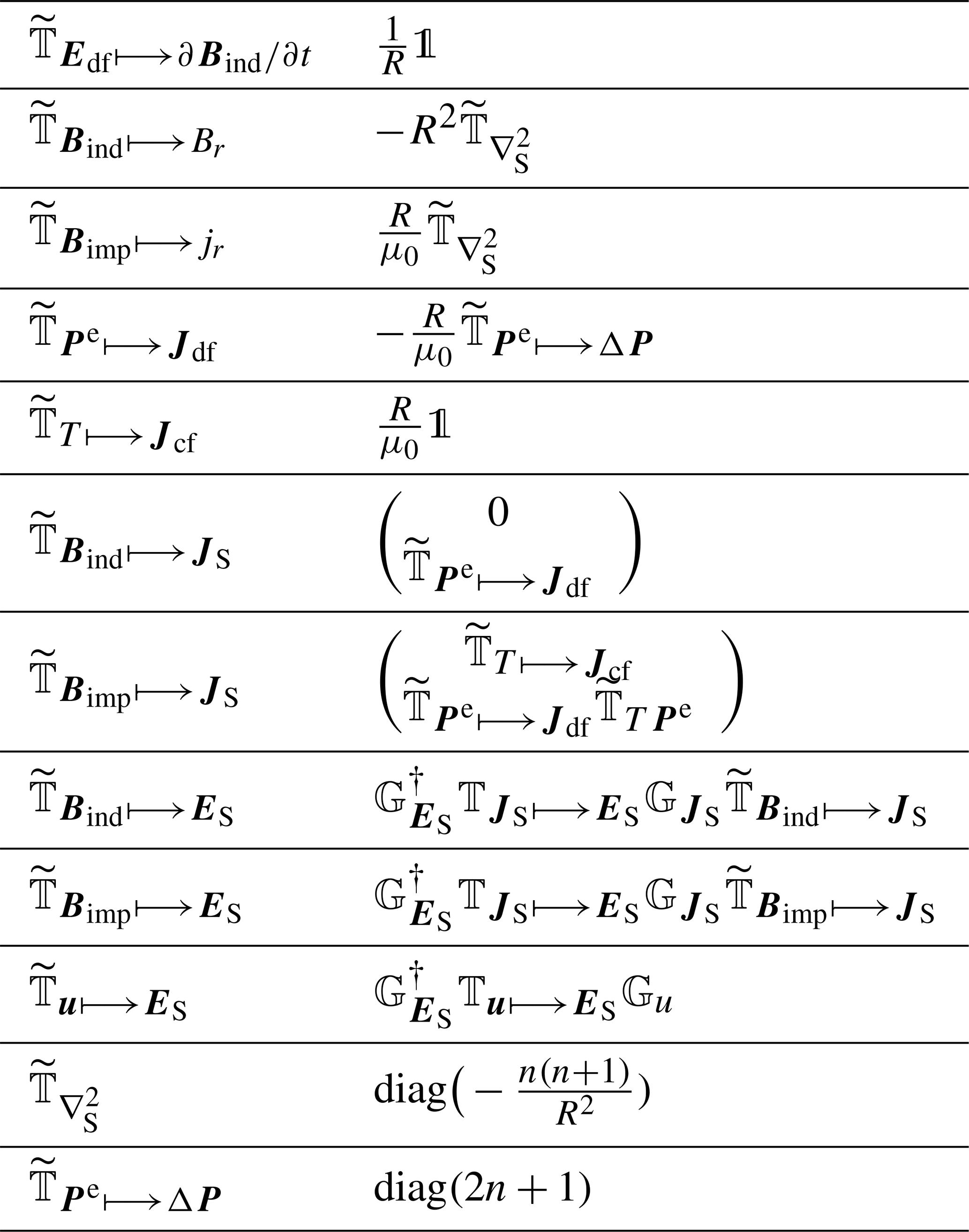
C4 Matrix Formulation of the Poloidal Magnetic Field of Field-Aligned Currents

In the numerical implementation, we represent Eq. (34), based on Engels and Olsen (1998), as a matrix ${\stackrel{\mathrm{̃}}{\mathbb{T}}}_{{\mathit{B}}_{\mathrm{imp}}\mapsto {\mathit{P}}^{\mathrm{e}}}$ that transforms vectors of toroidal spherical harmonic coefficients to corresponding vectors of spherical harmonic coefficients of external poloidal fields. This is done by performing the discretized integration of poloidal magnetic field contributions from the horizontal components of the field-aligned currents at r>R via the midpoint rule

$$\begin{array}{}\text{(C37)}& {\stackrel{\mathrm{̃}}{\mathbb{T}}}_{{\mathit{B}}_{\mathrm{imp}}\mapsto {\mathit{P}}^{\mathrm{e}}}=-\mathrm{\Delta }r\sum _{i=\mathrm{1}}^N{\stackrel{\mathrm{̃}}{\mathbb{T}}}_{{\mathit{P}}^{\mathrm{e}}\left(r_i\right)\mapsto {\mathit{P}}^{\mathrm{e}}}{\stackrel{\mathrm{̃}}{\mathbb{T}}}_{{\mathit{B}}_{\mathrm{imp}}\mapsto {\mathit{P}}^{\mathrm{e}}\left(r_i\right)}\end{array}$$

where the $r_i=R+\mathrm{\Delta }r/\mathrm{2}$ are the integration radii. The matrix

$$\begin{array}{}\text{(C38)}& {\stackrel{\mathrm{̃}}{\mathbb{T}}}_{{\mathit{P}}^{\mathrm{e}}\left(r_i\right)\mapsto {\mathit{P}}^{\mathrm{e}}}=\mathrm{diag}\left[{\left({\displaystyle \frac{R}{r_i}}\right)}^{n-\mathrm{1}}\right]\end{array}$$

represents the conversion of the spherical harmonic coefficients of an external poloidal field at radius r_i to radius R. The matrix ${\stackrel{\mathrm{̃}}{\mathbb{T}}}_{{\mathit{B}}_{\mathrm{imp}}\mapsto {\mathit{P}}^{\mathrm{e}}\left(r_i\right)}$ constructs the external poloidal field associated with the horizontal components of the field-aligned current density at r_i, and can be written as

$$\begin{array}{}\text{(C39)}& {\stackrel{\mathrm{̃}}{\mathbb{T}}}_{{\mathit{B}}_{\mathrm{imp}}\mapsto {\mathit{P}}^{\mathrm{e}}\left(r_i\right)}={\stackrel{\mathrm{̃}}{\mathbb{T}}}_{{\mathit{j}}_{\mathrm{h}}\left(r_i\right)\mapsto {\mathit{P}}^{\mathrm{e}}\left(r_i\right)}{\mathbb{G}}_{{\mathit{j}}_{\mathrm{h}}\left(r_i\right)}^{\mathit{†}}{\mathbb{T}}_{j_r\mapsto {\mathit{j}}_{\mathrm{h}}\left(r_i\right)}{\mathbb{G}}_{j_r}{\stackrel{\mathrm{̃}}{\mathbb{T}}}_{{\mathit{B}}_{\mathrm{imp}}\mapsto j_r}.\end{array}$$

${\stackrel{\mathrm{̃}}{\mathbb{T}}}_{{\mathit{B}}_{\mathrm{imp}}\mapsto j_r}$ transforms spherical harmonic coefficients of the imposed magnetic field to coefficients for the scalar j_r immediately above the ionosphere, and is given in Table C1. ${\mathbb{G}}_{j_r}$ evaluates the spherical harmonic expansion of j_r at cubed-sphere grid points according to Eq. (C1). In this work, we use the same $\mathrm{6}\times \mathrm{100}\times \mathrm{100}$ cubed-sphere grid for this calculation as used when calculating the matrices in Sect. C3. ${\mathbb{T}}_{j_r\mapsto {\mathit{j}}_{\mathrm{h}}\left(r_i\right)}$ represents the mapping of the grid-evaluated j_r to the corresponding grid-evaluated j_h at r=r_i via Eq. (36). The Moore-Penrose inverse ${\mathbb{G}}_{{\mathit{j}}_{\mathrm{h}}\left(r_i\right)}^{\mathit{†}}$ performs a minimum-norm least-squares spherical harmonic decomposition of the horizontal current density at the mapped grid points at r=r_i according to Eq. (C2), and ${\stackrel{\mathrm{̃}}{\mathbb{T}}}_{{\mathit{j}}_{\mathrm{h}}\left(r_i\right)\mapsto {\mathit{P}}^{\mathrm{e}}\left(r_i\right)}={\stackrel{\mathrm{̃}}{\mathbb{T}}}_{{\mathit{B}}_{\mathrm{ind}}\mapsto {\mathit{J}}_{\mathrm{S}}}^{-\mathrm{1}}$ converts the coefficients into corresponding coefficients of an external poloidal magnetic field with r_i as the reference radius, where ${\stackrel{\mathrm{̃}}{\mathbb{T}}}_{{\mathit{B}}_{\mathrm{ind}}\mapsto {\mathit{J}}_{\mathrm{S}}}$ is given in Table C1.