An empirical model of high-latitude ionospheric conductances based on EISCAT observations

Conductances are key properties of the ionospheric electrodynamics and the difficulty of measuring them directly is a significant limitation to the usefulness of many analysis techniques. We have utilized all available field-aligned observations from the EISCAT incoherent scatter ultra-high frequency (UHF) radar since 2001 and from the 42 m EISCAT Svalbard Radar (ESR) since 1998 to develop a new empirical model for estimating the high-latitude ionospheric Hall and Pedersen conductances. The solar radiation component of the model is parametrized with the solar zenith angle and the F_10.7 index, and the auroral precipitation component is parametrized with the magnetic local time and the divergence-free part of the horizontal ionospheric current density, which is obtained from ground-based magnetic field observations. We have also derived a new technique based on spherical elementary current systems that can be used to solve for the ionospheric potential electric field and field-aligned current density from known ionospheric conductances and ground-based magnetic field observations, taking into account induction in the ionosphere and in the ground. The new empirical conductance model and solver were applied to IMAGE magnetometer network observations. Comparison of the results with Swarm and Active Magnetosphere and Planetary Electrodynamics Response Experiment (AMPERE) satellite observations showed reasonable agreement in the electric field profile and direction of the field-aligned current, but in the post-midnight sector the modelled amplitudes tended to be weaker than observations. The combination of the new conductance model and analysis technique allows estimating the key properties of ionospheric electrodynamics from ground-based magnetic field observations.

1 Introduction

Key properties of the ionospheric electrodynamics are electric fields, currents, and height-integrated conductivities, also called conductances. They are tightly coupled to adjacent domains: Field-aligned currents and the potential electric field connect the ionosphere and the magnetosphere, providing a window to processes in the vast and distant near-Earth space through observations of the more compact and conveniently located ionosphere. Joule heating due to the currents affects thermospheric density, with poorly understood but occasionally disastrous effects on satellite orbits (e.g., Zhang et al., 2022). The inductive electric field interacts with the conducting ground (e.g., Juusola et al., 2025b), driving potentially hazardous geomagnetically induced currents (GICs) in technological conductor networks.

A crucial limitation to studying ionospheric electrodynamics is the scarcity of simultaneous observations of the key properties of ionospheric electrodynamics in the same region. Long time series of observations at a comparable and sufficiently detailed spatial and temporal resolution would be ideal, in order to cover all relevant event types. Global or even regional observations of the ionospheric conductance distribution are especially difficult to obtain (see, e.g., Robinson et al., 2020; Palmroth et al., 2021; Wang and Zou, 2022). However, at large spatial scales (∼1000 km) and 10 min time resolution, Green et al. (2007) suggest that they could be estimated by combining the ionospheric currents from SuperMAG (Gjerloev, 2012) and Active Magnetosphere and Planetary Electrodynamics Response Experiment (AMPERE; Anderson et al., 2002) observations and the electric field from Super Dual Auroral Radar Network (SuperDARN; Chisham et al., 2007) observations.

The International Monitor for Auroral Geomagnetic Effects (IMAGE) magnetometer network, located in Fennoscandia and surrounding areas, provides a continuous time series of meso-scale (∼100 km), 10 s ground-based magnetic field observations that cover several solar cycles. From these data, it is possible to derive the divergence-free (DF) part of the horizontal current density J_DF and the DF (i.e., inductive) part of the horizontal ionospheric electric field E_DF due to telluric and DF ionospheric currents (Pirjola and Viljanen, 1998; Madelaire et al., 2024; Juusola et al., 2025b). Above the ionospheric horizontal current sheet, the curl-free (CF) horizontal ionospheric currents and field-aligned currents also contribute to the DF electric field, although Vanhamäki et al. (2007) argue that this DF electric field should be very small.

There are no regional potential electric field data available in the IMAGE area. However, if ionospheric conductances were available, the CF part of the horizontal electric field E_CF (i.e., potential electric field) and the CF part of the horizontal current density J_CF could be calculated using the expressions from Juusola et al. (2025b),

$$\begin{array}{}\text{(1)}& {\displaystyle }\mathit{E}={\mathit{E}}_{\text{CF}}+{\mathit{E}}_{\text{DF}}\text{(2)}& {\displaystyle }\mathit{J}={\mathit{J}}_{\text{CF}}+{\mathit{J}}_{\text{DF}}\text{(3)}& {\displaystyle }\mathit{J}={\mathrm{\Sigma }}_{\mathrm{P}}\mathit{E}+{\mathrm{\Sigma }}_{\mathrm{H}}\mathit{E}\times {\widehat{\mathit{e}}}_{\mathrm{r}}\text{(4)}& {\displaystyle }\begin{array}{rl}(\mathrm{\nabla }\times \mathit{J}{)}_{\mathrm{r}}=& [\mathrm{\nabla }{\mathrm{\Sigma }}_{\mathrm{P}}\times ({\mathit{E}}_{\text{CF}}+{\mathit{E}}_{\text{DF}}){]}_{\mathrm{r}}+{\mathrm{\Sigma }}_{\mathrm{P}}[\mathrm{\nabla }\times {\mathit{E}}_{\text{DF}}{]}_{\mathrm{r}}\\ & +[\mathrm{\nabla }{\mathrm{\Sigma }}_{\mathrm{H}}\times (({\mathit{E}}_{\text{CF}}+{\mathit{E}}_{\text{DF}})\times {\widehat{\mathit{e}}}_{\mathrm{r}}){]}_{\mathrm{r}}\\ & -{\mathrm{\Sigma }}_{\mathrm{H}}(\mathrm{\nabla }\cdot {\mathit{E}}_{\text{CF}})\end{array}\text{(5)}& {\displaystyle }\begin{array}{rl}\mathrm{\nabla }\cdot \mathit{J}=& \mathrm{\nabla }{\mathrm{\Sigma }}_{\mathrm{P}}\cdot ({\mathit{E}}_{\text{CF}}+{\mathit{E}}_{\text{DF}})+{\mathrm{\Sigma }}_{\mathrm{P}}\mathrm{\nabla }\cdot {\mathit{E}}_{\text{CF}}\\ & +\mathrm{\nabla }{\mathrm{\Sigma }}_{\mathrm{H}}\cdot \left[\right({\mathit{E}}_{\text{CF}}+{\mathit{E}}_{\text{DF}})\times {\widehat{\mathit{e}}}_{\mathrm{r}}]\\ & +{\mathrm{\Sigma }}_{\mathrm{H}}(\mathrm{\nabla }\times {\mathit{E}}_{\text{DF}}{)}_{\mathrm{r}}.\end{array}\end{array}$$

Here, J is the ionospheric sheet current density perpendicular to the main magnetic field, E is the electric field perpendicular to the magnetic field, Σ_P is the Pedersen conductance perpendicular to the magnetic field and parallel to the eletric field, Σ_H is the Hall conductance perpendicular to both the magnetic and electric field, and ${\widehat{\mathit{e}}}_{\mathrm{r}}$ is a unit vector in the direction of the assumed radial magnetic field lines. This approach has a similar basis as the KRM technique (Kamide et al., 1981), the Assimilative Mapping of Ionospheric Electrodynamics (AMIE; Richmond and Kamide, 1988; Richmond, 1992), and Local Mapping of Polar Ionospheric Electrodynamics (Lompe; Laundal et al., 2022a), but unlike those models, it takes E_DF into account as well. In some dynamical situations, inductive effects are not negligible and the ionospheric electric field is not a pure CF field, but can have a significant DF part (Vanhamäki et al., 2007; Madelaire et al., 2024).

There are two main sources of Σ_P and Σ_H: photoionization, which is caused by solar radiation on the dayside, and impact ionization, which is caused by auroral precipitation. Moen and Brekke (1993) have derived an empirical model for the solar radiation component as a function of the solar zenith angle χ and F_10.7 solar flux based on nine days of data from the European Incoherent Scatter Scientific Association (EISCAT) incoherent scatter radar. Another model with slightly different parametrization was developed by Ieda et al. (2015). Ahn et al. (1998), on the other hand, have derived an empirical model for the precipitation components of Σ_P and Σ_H as a function of horizontal and vertical ground magnetic field perturbations and magnetic local time (MLT) based on auroral-zone Chatanika incoherent scatter radar data. This model has been incorporated into AMIE.

We will utilize a newly processed data set of Σ_P and Σ_H, derived from all available field-aligned EISCAT Ultra High Frequency (UHF) radar observations between January 2001 and January 2024 and from the 42 m EISCAT Svalbard Radar (ESR) between October 1998 and January 2024, to continue the work of Moen and Brekke (1993) and Ahn et al. (1998). The UHF radar is located in Tromsø in Northern Norway and the ESR radar near Longyearbyen in Svalbard. Our aim is to develop an empirical model for Σ_P and Σ_H that would make it possible to estimate E_CF and J_CF from J_DF and E_DF. Instead of ground magnetic field variations, which are often contaminated by signatures from induced telluric currents (Juusola et al., 2020), we will use the ionospheric J_DF to parametrize the precipitation-dependent component. Furthermore, we will show that the empirical model of Moen and Brekke (1993), which is based on nine days of EISCAT data, is not ideal for describing the newly processed, long time series of EISCAT conductances, and derive a new, modified version by simultanously fitting both the solar radiation and precipitation component models to the observations.

An empirical model that predicts the precipitation component of Σ_P and Σ_H based on J_DF has the advantage that the conductances have the same spatial resolution as J_DF, and they follow the dynamics of J_DF, unlike for example climatological models that use some other parameter as input (e.g., Newell et al., 2009; Machol et al., 2012; Hatch et al., 2024). Furthermore, the time series is not truncated due to dependency on data from another instrument. In the near future, EISCAT_3D will start operations in northern Fennoscandia and provide detailed, volumetric observations of the ionospheric conductivities and electric fields. Our model can provide meso-scale context to the regionally more limited EISCAT_3D observations.

The structure of the study is as follows: the data and methods are described in Sect. 2, the empirical model is developed and validated in Sect. 3, and its performance is discussed in Sect. 4. The conclusions are summarised in Sect. 5.

2 Data and methods

2.1 EISCAT radar data

2.1.1 Data selection

All data available from the EISCAT UHF radar in Tromsø from January 2001 to January 2024 and from the 42 m ESR near Longyearbyen from October 1998 to January 2024 were downloaded from the Madrigal data base (Madrigal, 2025). UHF data measured before a major system upgrade in 2000 were not used, because the amount of data in Madrigal is very small and the radar modes and data analysis were different from those used after the upgrade. Data less than one year old in January 2025 were not used due to the embargo rules of EISCAT. The EISCAT data in Madrigal are plasma parameters fitted to measured incoherent scatter spectra using the Grand Unified Incoherent Scatter Design and Analysis Program (GUISDAP; Lehtinen and Huuskonen, 1996; Häggström, 2025). The fitted parameters are electron density (N_e), electron temperature, ion temperature, and line-of-sight bulk plasma velocity. In this study, we use electron densities, and select only electron density profiles measured with a magnetic field aligned radar beam and with 30 to 120 s time resolution. The profiles were cleaned by removing individual data points according to the following conditions: the GUISDAP fit must be flagged as successful, relative error in N_e must be smaller than 0.5, chi-square of the fit must be smaller than 10, ion temperature must be larger than 50 K, and N_e<10¹² m⁻³ below 95 km altitude. The last two conditions remove clearly erroneous results that are not captured automatically by GUISDAP. Logarithm of N_e was then linearly interpolated to 1 km range resolution between 75 and 330 km altitudes to create a consistent data set. Range resolution of the fitted plasma parameters depends on altitude and may vary between radar modes. The resolution is typically about 3 km in the lower E region (below 110 km altitude) and about 20 km at 330 km altitude. Finally, profiles that contain electron densities larger than 5×10¹² m⁻³ after the interpolation were rejected to remove strong, non-ionospheric echoes, e.g., from satellites. The limit was chosen to be close to, but clearly above, the largest density one may realistically expect in the F region. The test was done only for the interpolated data up to 330 km altitude. Also satellites above 330 km altitude may affect the densities measured below 330 km, because satellite echoes from above may be aliased below 330 km in the radar signal processing. The fraction of profiles rejected based on this criterion was 0.066 % for the UHF and 0.035 % for the ESR.

2.1.2 Conductivity calculation

Hall and Pedersen conductivities σ_H and σ_P were calculated from the interpolated N_e as

$$\begin{array}{}\text{(6)}& {\displaystyle }& {\displaystyle }{\mathit{\sigma }}_{\mathrm{P}}=\left({\displaystyle \frac{\mathrm{1}}{m_{\mathrm{e}}{\mathit{\nu }}_{\text{en}}}}{\displaystyle \frac{{\mathit{\nu }}_{\text{en}}^{\mathrm{2}}}{{\mathit{\nu }}_{\text{en}}^{\mathrm{2}}+{\mathit{\omega }}_{\text{ce}}^{\mathrm{2}}}}+{\displaystyle \frac{\mathrm{1}}{m_{\mathrm{i}}{\mathit{\nu }}_{\text{in}}}}{\displaystyle \frac{{\mathit{\nu }}_{\text{in}}^{\mathrm{2}}}{{\mathit{\nu }}_{\text{in}}^{\mathrm{2}}+{\mathit{\omega }}_{\text{ci}}^{\mathrm{2}}}}\right)N_{\mathrm{e}}{e}^{\mathrm{2}}\text{(7)}& {\displaystyle }& {\displaystyle }{\mathit{\sigma }}_{\mathrm{H}}=\left({\displaystyle \frac{\mathrm{1}}{m_{\mathrm{e}}{\mathit{\nu }}_{\text{en}}}}{\displaystyle \frac{{\mathit{\omega }}_{\text{ce}}{\mathit{\nu }}_{\text{en}}}{{\mathit{\nu }}_{\text{en}}^{\mathrm{2}}+{\mathit{\omega }}_{\text{ce}}^{\mathrm{2}}}}-{\displaystyle \frac{\mathrm{1}}{m_{\mathrm{i}}{\mathit{\nu }}_{\text{in}}}}{\displaystyle \frac{{\mathit{\omega }}_{\text{ci}}{\mathit{\nu }}_{\text{in}}}{{\mathit{\nu }}_{\text{in}}^{\mathrm{2}}+{\mathit{\omega }}_{\text{ci}}^{\mathrm{2}}}}\right)N_{\mathrm{e}}{e}^{\mathrm{2}},\end{array}$$

where m_e and m_i are the electron and ion mass, e is the unit charge, ω_ce and ω_ci are the cyclotron or gyrofrequency of electrons and ions, and ν_en and ν_in are the electron-neutral and ion-neutral collision frequencies (Schunk and Nagy, 2009).

First, neutral atmospheric parameters were obtained using the NRLMSISE-00 model (Picone et al., 2002) for the location and time of each measurement. Ion-neutral collision frequencies for molecular ions (75 % NO⁺ and 25 % ${\mathrm{O}}_{\mathrm{2}}^{+}$), atomic ions (O⁺), and electron-neutral collision frequencies were calculated using formulas of Schunk and Nagy (2009). The NRLMSISE-00 neutral temperature (T_n) was used for ion (T_i) and electron (T_e) temperatures ($T_{\mathrm{i}}=T_{\mathrm{e}}=T_{\mathrm{n}}$), because the fitted T_i and T_e are often very noisy, especially when N_e is low. T_e and T_i may be increased above T_n by particle precipitation and Joule heating, respectively. Although the ion-neutral collisions frequencies of Schunk and Nagy (2009) are temperature dependent, Baloukidis et al. (2023) reported that doubling the model T_n has only a very small effect on the Pedersen conductance estimates. We have made a similar test for both Pedersen and Hall conductances, and found that doubling T_e, T_i, or both has only very small effect on both Pedersen and Hall conductances.

Magnetic field intensities were calculated with the International Geomagnetic Reference Field (IGRF-13) model (Alken et al., 2021), and these were used to calculate gyrofrequencies. Pedersen and Hall conductivities were calculated using the modelled collision frequencies and gyrofrequencies, the measured N_e, and molecular-to-atomic ion density ratio from the International Reference Ionosphere (IRI) model (Bilitza et al., 2022). Standard deviations (STD) of the conductivities were calculated using STD of N_e from the GUISDAP fits, which is expected to be the dominant source of error. The model values of collision frequencies and gyrofrequencies, which are based on well-established models of the geomagnetic field and the neutral atmosphere, were considered exact.

2.1.3 Height integration and final cleaning

Hall and Pedersen conductances were height-integrated from the conductivities, except if the profile contained extremely small ($N_{\mathrm{e}}<{\mathrm{10}}^{q_{\mathrm{1}}-\mathrm{0.2}}$, where q₁ is the 0.001 quantile of the log ₁₀(N_e) values) or large ($N_{\mathrm{e}}>{\mathrm{10}}^{q_{\mathrm{2}}+\mathrm{0.2}}$, where q₂ is the 0.999 quantile of the log ₁₀(N_e) values) N_e. This was done in order to remove strong satellite echoes. All data were plotted, and radar experiments that suffered from obvious technical problems or did not have sufficient altitude coverage for the conductance calculation were manually removed. Duplicate analysis runs of the same data were also removed.

Remaining satellite echoes and noise spikes (or minima) caused by technical issues were removed as follows: For both Pedersen and Hall conductances, the standard deviation and mean of data points within 10 points from point i in the time series, excluding point i, were calculated. Point i was flagged as a noise spike, if either of the conductances at point i deviated more than 10 standard deviations from the corresponding mean values. All rejected points were removed from the final data vectors.

Pedersen and Hall conductivity data points where the N_e profiles did not reach low enough altitudes were rejected if the following conditions were satisfied: (1) Conductivity at the lowest measured altitude was more than $\mathrm{2}\times {\mathrm{10}}^{-\mathrm{4}}$ S m⁻¹ or more than half of the maximum conductivity. (2) The conductivity maximum was located less than 5 km above the lowest measured altitude. In the end, we were left with 609 776 Σ_P values and 605 774 Σ_H values from UHF and 925 900 Σ_P values and 923 638 Σ_H values from ESR. Their magnetic local time distributions are illustrated in Figs. 3e and 4e. These figures will be discussed in more detail in Sect. 3.1.

2.2 IMAGE magnetometer network data

We have used 10 s ground magnetic field measurements from the IMAGE magnetometers (Juusola et al., 2025a). For data before 2015, we have used the method by van de Kamp (2013) to subtract the long-term baseline (including instrument drifts, etc.), any jumps in the data, and the diurnal variation from the variometer data. For 2015 onwards, we have first corrected the data for any jumps and spikes and then subtracted a ten-day sliding median. The ten-day sliding median was calculated for the midnight of each day and the baseline values in between were interpolated using a cosine curve.

The remaining variation magnetic field consists of an external part mainly due to ionospheric electric currents but with some magnetospheric contribution as well, and an internal part due to induced telluric currents in the conducting ground. We have used the two-dimensional (2D) Spherical Elementary Current System (SECS) method (Amm, 1997; Amm and Viljanen, 1999; Pulkkinen et al., 2003a, b; McLay and Beggan, 2010; Weygand et al., 2011; Marsal et al., 2017, 2020; Laundal et al., 2021; Vanhamäki and Juusola, 2020; Walker et al., 2023; Juusola et al., 2016b, 2020, 2023a, b, 2025b) to estimate the ionospheric J_DF for the time integration intervals of EISCAT Σ_P and Σ_H at the locations of the field-aligned measurements, (69.583°, 19.210°) geodetic latitude and longitude for UHF and (78.09°, 16.02°) for ESR. For each value of Σ_P and Σ_H, the corresponding value of J_DF was obtained as a mean of the J_DF values during the radar measurement integration time.

2.3 Ionospheric electrodynamics with the 2D SECS method

The divergence-free part of the ionospheric horizontal current density can be expressed in terms of 2D DF SECS functions. The current density of the divergence-free (DF) 2D SECS is

$$\begin{array}{}\text{(8)}& {\mathit{J}}_{\text{DF}}(t,{\mathit{\theta }}^{\prime })={\displaystyle \frac{I_{\text{DF}}\left(t\right)}{\mathrm{4}\mathit{\pi }R}}{\widehat{\mathit{e}}}_{{\mathit{\varphi }}^{\prime }}\left\{\begin{array}{ll}\tan \left(\frac{{\mathit{\theta }}^{\prime }}{\mathrm{2}}\right){\cot }^{\mathrm{2}}\left(\frac{{\mathit{\theta }}_{\mathrm{0}}}{\mathrm{2}}\right),& {\mathit{\theta }}^{\prime }<{\mathit{\theta }}_{\mathrm{0}}\\ \cot \left(\frac{{\mathit{\theta }}^{\prime }}{\mathrm{2}}\right),& {\mathit{\theta }}^{\prime }\ge {\mathit{\theta }}_{\mathrm{0}}\end{array}\right.\end{array}$$

where R is the radius of the ionosphere, θ^′ is the colatitude in the SECS coordinates, ${\widehat{\mathit{e}}}_{{\mathit{\varphi }}^{\prime }}$ is a unit vector in the zonal direction in the SECS coordinates, and I_DF(t) is the time-dependent DF SECS amplitude. The curl of J_DF is uniformly distributed over a spherical cap defined by the colatitude θ₀

$$\begin{array}{}\text{(9)}& (\mathrm{\nabla }\times {\mathit{J}}_{\text{DF}}{)}_{\mathrm{r}}=-{\displaystyle \frac{I_{\text{DF}}\left(t\right)}{\mathrm{4}\mathit{\pi }{R}^{\mathrm{2}}}}+\left\{\begin{array}{ll}\frac{I_{\text{DF}}\left(t\right)}{A},& {\mathit{\theta }}^{\prime }<{\mathit{\theta }}_{\mathrm{0}}\\ \mathrm{0},& {\mathit{\theta }}^{\prime }\ge {\mathit{\theta }}_{\mathrm{0}}\end{array}\right.\end{array}$$

where A is the area of the spherical cap,

$$\begin{array}{}\text{(10)}& A=\mathrm{2}\mathit{\pi }{R}^{\mathrm{2}}(\mathrm{1}-\cos {\mathit{\theta }}_{\mathrm{0}})\end{array}$$

and can be set to equal the SECS grid cell area. The magnetic field associated with J_DF is

$$\begin{array}{ll}\text{(11)}& {\displaystyle }\mathit{B}=& {\displaystyle }{B}_{\mathrm{r}}{\widehat{\mathit{e}}}_{\mathrm{r}}+B_{{\mathit{\theta }}^{\prime }}{\widehat{\mathit{e}}}_{{\mathit{\theta }}^{\prime }}{\displaystyle }{B}_{\mathrm{r}}(t,r,{\mathit{\theta }}^{\prime })=& {\displaystyle \frac{I_{\text{DF}}\left(t\right){\mathit{\mu }}_{\mathrm{0}}}{\mathrm{4}\mathit{\pi }}}{\displaystyle \frac{\mathrm{1}}{r}}\left({\displaystyle \frac{R}{\sqrt{r^{\mathrm{2}}-\mathrm{2}rR\cos {\mathit{\theta }}^{\prime }+R^{\mathrm{2}}}}}\right.\\ \text{(12)}& {\displaystyle }& {\displaystyle }\left.+\left\{\begin{array}{ll}-\mathrm{1},& r<R\\ -R/r,& r\ge R\end{array}\right.\right){\displaystyle }{B}_{{\mathit{\theta }}^{\prime }}(t,r,{\mathit{\theta }}^{\prime })=& {\displaystyle }-{\displaystyle \frac{I_{\text{DF}}\left(t\right){\mathit{\mu }}_{\mathrm{0}}}{\mathrm{4}\mathit{\pi }}}{\displaystyle \frac{\mathrm{1}}{r\sin {\mathit{\theta }}^{\prime }}}\left({\displaystyle \frac{r-R\cos {\mathit{\theta }}^{\prime }}{\sqrt{r^{\mathrm{2}}-\mathrm{2}rR\cos {\mathit{\theta }}^{\prime }+R^{\mathrm{2}}}}}\right.\\ \text{(13)}& {\displaystyle }& {\displaystyle }\left.+\left\{\begin{array}{ll}\cos {\mathit{\theta }}^{\prime },& r<R\\ -\mathrm{1},& r>R\end{array}\right.\right)\end{array}$$

where μ₀ is the vacuum permeability. There is a small inconsistency between the magnetic field of Eqs. (12)–(13) and the current density of Eq. (8), because the magnetic field expressions have been derived for θ₀=0. However, as discussed by Vanhamäki and Juusola (2020), this does not appear to affect practical applications.

The DF SECS poles are placed on uniform or nonuniform grids in the region of interest. With IMAGE we typically use grids with 0.5° latitude and 1° longitude resolution at 1 m depth and at 90 km altitude. The amplitudes I_DF are determined by fitting the superposed magnetic field of the SECSs to the three components of the measured magnetic field. Using the two DF SECS layers, one at 1 m depth and the other at 90 km altitude, will separate the external and internal contributions to the magnetic field variations. The inductive electric field associated with temporal changes in the J_DF amplitude is given by Faraday's law

$$\begin{array}{}\text{(14)}& (\mathrm{\nabla }\times {\mathit{E}}_{\text{DF}}{)}_{\mathrm{r}}=-{\displaystyle \frac{\partial B_{\mathrm{r}}}{\partial t}}\end{array}$$

as

$$\begin{array}{ll}{\displaystyle }{\mathit{E}}_{\text{DF}}(t,r,{\mathit{\theta }}^{\prime })=& {\displaystyle }-{\displaystyle \frac{\partial I_{\text{DF}}\left(t\right)}{\partial t}}{\displaystyle \frac{{\mathit{\mu }}_{\mathrm{0}}}{\mathrm{4}\mathit{\pi }}}{\widehat{\mathit{e}}}_{{\mathit{\varphi }}^{\prime }}{\displaystyle \frac{\mathrm{1}}{r\sin {\mathit{\theta }}^{\prime }}}\\ {\displaystyle }& {\displaystyle }\times \left(\sqrt{r^{\mathrm{2}}-\mathrm{2}rR\cos {\mathit{\theta }}^{\prime }+R^{\mathrm{2}}}\right.\\ \text{(15)}& {\displaystyle }& {\displaystyle }\left.+\left\{\begin{array}{ll}r\cos {\mathit{\theta }}^{\prime }-R,& r<R\\ R\cos {\mathit{\theta }}^{\prime }-r,& r\ge R\end{array}\right.\right)\end{array}$$

(Juusola et al., 2025b). The time derivative of the SECS amplitudes can be estimated as

$$\begin{array}{}\text{(16)}& {\displaystyle \frac{\partial I_{\text{DF}}}{\partial t}}\approx {\displaystyle \frac{I_{\text{DF}}\left(t\right)-I_{\text{DF}}(t-\mathrm{\Delta }t)}{\mathrm{\Delta }t}},\end{array}$$

where Δt is the time step of the data, 10 s for IMAGE. The DF SECS amplitudes of the telluric equivalent current sheet at 1 m depth can be used to calculate the internal contribution to E_DF and the DF SECS amplitudes of the ionospheric equivalent current sheet at 90 km altitude can be used to calculate the external contribution to E_DF. The total E_DF is then obtained as a sum of the internal and external contributions.

The curl-free (CF) part of the horizontal ionospheric current density can be expressed in terms of CF 2D SECS functions,

$$\begin{array}{}\text{(17)}& {\displaystyle }& {\displaystyle }{\displaystyle }{\mathit{J}}_{\text{CF}}(t,{\mathit{\theta }}^{\prime })={\displaystyle \frac{I_{\text{CF}}\left(t\right)}{\mathrm{4}\mathit{\pi }R}}{\widehat{\mathit{e}}}_{{\mathit{\theta }}^{\prime }}\left\{\begin{array}{ll}\tan \left(\frac{{\mathit{\theta }}^{\prime }}{\mathrm{2}}\right){\cot }^{\mathrm{2}}\left(\frac{{\mathit{\theta }}_{\mathrm{0}}}{\mathrm{2}}\right),& {\mathit{\theta }}^{\prime }<{\mathit{\theta }}_{\mathrm{0}}\\ \cot \left(\frac{{\mathit{\theta }}^{\prime }}{\mathrm{2}}\right),& {\mathit{\theta }}^{\prime }\ge {\mathit{\theta }}_{\mathrm{0}}\end{array}\right.\text{(18)}& {\displaystyle }& {\displaystyle }\mathrm{\nabla }\cdot {\mathit{J}}_{\text{CF}}=-j_{\mathrm{r}}=-{\displaystyle \frac{I_{\text{CF}}\left(t\right)}{\mathrm{4}\mathit{\pi }{R}^{\mathrm{2}}}}+\left\{\begin{array}{ll}\frac{I_{\text{CF}}\left(t\right)}{A},& {\mathit{\theta }}^{\prime }<{\mathit{\theta }}_{\mathrm{0}}\\ \mathrm{0},& {\mathit{\theta }}^{\prime }\ge {\mathit{\theta }}_{\mathrm{0}}\end{array}\right.\end{array}$$

where I_CF is the CF SECS amplitude and j_r is the radial current density. The magnetic field of J_CF is

$$\begin{array}{ll}{\displaystyle }\mathit{B}(t,r,{\mathit{\theta }}^{\prime })& {\displaystyle }=-{\displaystyle \frac{{\mathit{\mu }}_{\mathrm{0}}{I}_{\text{CF}}\left(t\right)}{\mathrm{4}\mathit{\pi }r}}{\widehat{\mathit{e}}}_{{\mathit{\varphi }}^{\prime }}\\ \text{(19)}& {\displaystyle }& {\displaystyle }\times \left\{\begin{array}{ll}\mathrm{0},& r<R\\ \tan \left(\frac{{\mathit{\theta }}^{\prime }}{\mathrm{2}}\right){\cot }^{\mathrm{2}}\left(\frac{{\mathit{\theta }}_{\mathrm{0}}}{\mathrm{2}}\right),& r>R,{\mathit{\theta }}^{\prime }<{\mathit{\theta }}_{\mathrm{0}}\\ \cot \left(\frac{{\mathit{\theta }}^{\prime }}{\mathrm{2}}\right),& r>R,{\mathit{\theta }}^{\prime }\ge {\mathit{\theta }}_{\mathrm{0}}\end{array}\right..\end{array}$$

Similarly, the CF part of the ionospheric horizontal electric field can be expressed as a superposition of 2D CF SECS functions,

$$\begin{array}{}\text{(20)}& {\displaystyle }{\displaystyle }{\mathit{E}}_{\text{CF}}(t,{\mathit{\theta }}^{\prime })={\displaystyle \frac{Q_{\text{CF}}\left(t\right)}{\mathrm{4}\mathit{\pi }R}}{\widehat{\mathit{e}}}_{{\mathit{\theta }}^{\prime }}\left\{\begin{array}{ll}\tan \left(\frac{{\mathit{\theta }}^{\prime }}{\mathrm{2}}\right){\cot }^{\mathrm{2}}\left(\frac{{\mathit{\theta }}_{\mathrm{0}}}{\mathrm{2}}\right),& {\mathit{\theta }}^{\prime }<{\mathit{\theta }}_{\mathrm{0}}\\ \cot \left(\frac{{\mathit{\theta }}^{\prime }}{\mathrm{2}}\right),& {\mathit{\theta }}^{\prime }\ge {\mathit{\theta }}_{\mathrm{0}}\end{array}\right.\text{(21)}& {\displaystyle }\mathrm{\nabla }\cdot {\mathit{E}}_{\text{CF}}={\displaystyle \frac{\mathit{\rho }}{{\mathit{ϵ}}_{\mathrm{0}}}}=-{\displaystyle \frac{Q_{\text{CF}}\left(t\right)}{\mathrm{4}\mathit{\pi }{R}^{\mathrm{2}}}}+\left\{\begin{array}{ll}\frac{Q_{\text{CF}}\left(t\right)}{A}& {\mathit{\theta }}^{\prime }<{\mathit{\theta }}_{\mathrm{0}}\\ \mathrm{0},& {\mathit{\theta }}^{\prime }\ge {\mathit{\theta }}_{\mathrm{0}}\end{array}\right.\end{array}$$

where Q_CF is the CF SECS amplitude, ρ is the charge density, and ϵ₀ is the vacuum permittivity. In addition to the CF electric field, it is often useful to determine the associated electric potential Φ_E,

$$\begin{array}{}\text{(22)}& {\displaystyle }{\mathit{E}}_{\text{CF}}(t,{\mathit{\theta }}^{\prime })=-\mathrm{\nabla }{\mathrm{\Phi }}_{\mathrm{E}}(t,{\mathit{\theta }}^{\prime })=-{\displaystyle \frac{\mathrm{1}}{R}}{\displaystyle \frac{\partial {\mathrm{\Phi }}_{\mathrm{E}}(t,{\mathit{\theta }}^{\prime })}{\partial {\mathit{\theta }}^{\prime }}}{\widehat{\mathit{e}}}_{{\mathit{\theta }}^{\mathbf{\prime }}}\text{(23)}& {\displaystyle }\begin{array}{rl}{\mathrm{\Phi }}_{\mathrm{E}}& (t,{\mathit{\theta }}^{\prime })=-R\underset{\mathrm{0}}{\overset{{\mathit{\theta }}^{\prime }}{\int }}{E}_{\text{CF},\mathit{\theta }}(t,\mathit{\theta })\mathrm{d}\mathit{\theta }={\displaystyle \frac{Q_{\text{CF}}\left(t\right)}{\mathrm{4}\mathit{\pi }}}\\ & \times \left\{\begin{array}{ll}{\cot }^{\mathrm{2}}\frac{{\mathit{\theta }}_{\mathrm{0}}}{\mathrm{2}}\ln \left({\cos }^{\mathrm{2}}\frac{{\mathit{\theta }}^{\prime }}{\mathrm{2}}\right),& {\mathit{\theta }}^{\prime }<{\mathit{\theta }}_{\mathrm{0}}\\ {\cot }^{\mathrm{2}}\frac{{\mathit{\theta }}_{\mathrm{0}}}{\mathrm{2}}\ln \left({\cos }^{\mathrm{2}}\frac{{\mathit{\theta }}_{\mathrm{0}}}{\mathrm{2}}\right)& \\ -\ln \left({\sin }^{\mathrm{2}}\frac{{\mathit{\theta }}^{\prime }}{\mathrm{2}}\right)+\ln \left({\sin }^{\mathrm{2}}\frac{{\mathit{\theta }}_{\mathrm{0}}}{\mathrm{2}}\right),& {\mathit{\theta }}^{\prime }\ge {\mathit{\theta }}_{\mathrm{0}}\end{array}\right.\end{array}\end{array}$$

where we have set ${\mathrm{\Phi }}_{\mathrm{E}}(t,\mathrm{0})=\mathrm{0}$.

If J_DF, E_DF, the Pedersen conductance Σ_P and the Hall conductance Σ_H are known, E_CF and J_CF can be determined using Eqs. (4) and (5). First, we write Eq. (4) in the form (cf. Juusola et al., 2025b)

$$\begin{array}{}\text{(24)}& {\displaystyle }\begin{array}{rl}{\displaystyle }\sum _j& {\displaystyle }\left[[-(\mathrm{\nabla }{\mathrm{\Sigma }}_{\mathrm{P}}{)}_{\mathit{\varphi },i}-\left(\mathrm{\nabla }{\mathrm{\Sigma }}_{\mathrm{H}}{)}_{\mathit{\theta },i}\right]g_{i,j}^{E_{\text{CF},\mathit{\theta }}}\right.\\ {\displaystyle }& {\displaystyle }\left.+\left[\right(\mathrm{\nabla }{\mathrm{\Sigma }}_{\mathrm{P}}{)}_{\mathit{\theta },i}-\left(\mathrm{\nabla }{\mathrm{\Sigma }}_{\mathrm{H}}{)}_{\mathit{\varphi },i}\right]g_{i,j}^{E_{\text{CF},\mathit{\varphi }}}+{\mathrm{\Sigma }}_{\mathrm{H},i}{\displaystyle \frac{\mathrm{1}}{\mathrm{4}\mathit{\pi }{R}^{\mathrm{2}}}}\right]Q_{\text{CF},j}\\ {\displaystyle }& {\displaystyle }-{\mathrm{\Sigma }}_{\mathrm{H},i}{\displaystyle \frac{Q_{\text{CF},i}}{A_i}}={\displaystyle \frac{I_{\text{DF},i}}{A_i}}-\sum _j{\displaystyle \frac{I_{\text{DF},j}}{\mathrm{4}\mathit{\pi }{R}^{\mathrm{2}}}}\\ {\displaystyle }& {\displaystyle }-\left[[-(\mathrm{\nabla }{\mathrm{\Sigma }}_{\mathrm{P}}{)}_{\mathit{\varphi },i}-\left(\mathrm{\nabla }{\mathrm{\Sigma }}_{\mathrm{H}}{)}_{\mathit{\theta },i}\right]E_{\text{DF},\mathit{\theta },i,j}\right.\\ {\displaystyle }& {\displaystyle }+\left[\right(\mathrm{\nabla }{\mathrm{\Sigma }}_{\mathrm{P}}{)}_{\mathit{\theta },i}-\left(\mathrm{\nabla }{\mathrm{\Sigma }}_{\mathrm{H}}{)}_{\mathit{\varphi },i}\right]E_{\text{DF},\mathit{\varphi },i,j}\\ {\displaystyle }& {\displaystyle }\left.+{\mathrm{\Sigma }}_{\mathrm{P}}(\mathrm{\nabla }\times {\mathit{E}}_{\text{DF}}{)}_{\mathrm{r}}\right].\end{array}\end{array}$$

Here, we have denoted the geometry-dependent components of E_CF (Eq. 20) by g. We can use this expression to solve for Q_CF,i, at grid points i. Writing Eq. (5) in the form

$$\begin{array}{}\text{(25)}& {\displaystyle }\begin{array}{rl}{\displaystyle \frac{I_{\text{CF},i}}{A_i}}& {\displaystyle }-\sum _j{\displaystyle \frac{I_{\text{CF},j}}{\mathrm{4}\mathit{\pi }{R}^{\mathrm{2}}}}=\\ {\displaystyle }& {\displaystyle }\sum _j\left[\left[\right(\mathrm{\nabla }{\mathrm{\Sigma }}_{\mathrm{P}}{)}_{\mathit{\theta },i}-\left(\mathrm{\nabla }{\mathrm{\Sigma }}_{\mathrm{H}}{)}_{\mathit{\varphi },i}\right]E_{\text{DF},\mathit{\theta },i,j}\right.\\ {\displaystyle }& {\displaystyle }\left.+\left[\right(\mathrm{\nabla }{\mathrm{\Sigma }}_{\mathrm{P}}{)}_{\mathit{\varphi },i}+\left(\mathrm{\nabla }{\mathrm{\Sigma }}_{\mathrm{H}}{)}_{\mathit{\theta },i}\right]E_{\text{DF},\mathit{\varphi },i,j}\right]\\ {\displaystyle }& {\displaystyle }+\sum _j\left[\left[\right(\mathrm{\nabla }{\mathrm{\Sigma }}_{\mathrm{P}}{)}_{\mathit{\theta },i}-\left(\mathrm{\nabla }{\mathrm{\Sigma }}_{\mathrm{H}}{)}_{\mathit{\varphi },i}\right]g_{i,j}^{E_{\text{CF},\mathit{\theta }}}\right.\\ {\displaystyle }& {\displaystyle }+\left[\right(\mathrm{\nabla }{\mathrm{\Sigma }}_{\mathrm{P}}{)}_{\mathit{\varphi },i}+\left(\mathrm{\nabla }{\mathrm{\Sigma }}_{\mathrm{H}}{)}_{\mathit{\theta },i}\right]g_{i,j}^{E_{\text{CF},\mathit{\varphi }}}\\ {\displaystyle }& {\displaystyle }\left.-{\mathrm{\Sigma }}_{\mathrm{P},i}{\displaystyle \frac{\mathrm{1}}{\mathrm{4}\mathit{\pi }{R}^{\mathrm{2}}}}\right]Q_{\text{CF},j}+{\mathrm{\Sigma }}_{P,i}{\displaystyle \frac{Q_{\text{CF},i}}{A_i}},\end{array}\end{array}$$

we can solve for the CF SECS amplitudes I_CF,i. The problem can be made more straightforward with the approximation

$$\begin{array}{}\text{(26)}& {\displaystyle \frac{I_{\text{CF},i}}{A_i}}-\sum _j{\displaystyle \frac{I_{\text{CF},j}}{\mathrm{4}\mathit{\pi }{R}^{\mathrm{2}}}}\approx {\displaystyle \frac{I_{\text{CF},i}}{A_i}}.\end{array}$$

Globally, the sum of all amplitudes is expected to be approximately zero. In local applications, the sum can be non-zero, but as it represents the global sum, more realistic results are in fact obtained by discarding the term.

2.4 Swarm data

2.4.1 Electric field

We have used the Python package viresclient (Smith et al., 2025) to access Swarm Thermal Ion Imager (TII) cross-track ion flow velocity (“Viy”) measurements, satellite velocity (“VsatC”, “VsatE”, “VsatN”), and geomagnetic field models (“B_NEC_CHAOS-Core”, “B_NEC_CHAOS-Static”, “B_NEC_CHAOS-MMA-Primary”, “B_NEC_CHAOS-MMA-Secondary”) from the European Space Agency's VirES for Swarm service (VirES, 2025). These data are available in the collection “SW_EXPT_EFIx_TCT02”, which is described to contain 2 Hz cross-track ion flows. We have only downloaded data northward of quasi-dipole latitude 44°, which is the low-latitude boundary used for EFI TII cross-track flow calibration, and data that are flagged calibrated, as indicated by the second bit of the quantity Quality_flags being set to 1 (Burchill and Knudsen, 2020). The measurements are provided in satellite track coordinates where the unit vector ${\widehat{\mathit{e}}}_x$ is in the direction of the satellite velocity, ${\widehat{\mathit{e}}}_z$ points radially downward, and ${\widehat{\mathit{e}}}_y=-{\widehat{\mathit{e}}}_x\times {\widehat{\mathit{e}}}_z$. The magnetic field model data are provided in the North-East-Centre (NEC) reference frame.

The electric field at Swarm altitude was obtained from the cross-track ion velocity V_i,y as $E_x=-V_{i,y}{B}_{\text{model,C}}$ and mapped to the altitude of the horizontal current sheet by multiplying by $\sqrt{B_{\text{IGRF},{\mathit{J}}_{\text{DF}}}/B_{\text{IGRF,sat}}}$, where the IGRF amplitude was obtained using Laundal et al. (2022b). The corresponding component from the IMAGE electric field north (E_N) and east (E_E) components was obtained as

$$\begin{array}{}\text{(27)}& E_x=E_{\mathrm{N}}{\displaystyle \frac{V_{\text{sat,N}}}{\sqrt{V_{\text{sat,N}}^{\mathrm{2}}+V_{\text{sat,E}}^{\mathrm{2}}}}}+E_{\mathrm{E}}{\displaystyle \frac{V_{\text{sat,E}}}{\sqrt{V_{\text{sat,N}}^{\mathrm{2}}+V_{\text{sat,E}}^{\mathrm{2}}}}}.\end{array}$$

The footpoints of the satellite observations at the altitude of the horizontal current sheet were traced along the IGRF field using the Apexpy code (Laundal et al., 2022b).

2.4.2 Field-aligned current density

We also obtained Swarm single satellite (SW_OPER_FACxTMS_2F) and dual-satellite (SW_OPER_FAC_TMS_2F) radial current measurements (“IRC”) (Ritter et al., 2013) as well as the auxilaries “F107”, “SunZenithAngle”, and “MLT”. Field-aligned current amplitudes were mapped from the satellite altitude to the altitude of the horizontal current sheet by multiplying them by $B_{\text{IGRF},{\mathit{J}}_{\text{DF}}}/B_{\text{IGRF,sat}}$, where the IGRF amplitude was obtained using Laundal et al. (2022b).

2.5 AMPERE field-aligned current density

We obtained Active Magnetosphere and Planetary Electrodynamics Response Experiment (AMPERE) radial current densities via the AMPERE Science Data Center (Anderson et al., 2025). The large-scale current densities are derived from the Iridium constellation perturbation magnetic field observations (Waters et al., 2020). Ten minutes of the observed magnetic perturbations are fitted with spherical harmonics, and the radial currents are derived as the curl of the spherical harmonic magnetic perturbation fit. The spherical harmonic fit is implemented over the entire sphere with a latitude order of 60, corresponding to a latitude resolution of 3°, and a longitude order of 5 commensurate with the orbit spacing. We mapped the AMPERE current density from the satellite altitude to the altitude of the horizontal current sheet as described in Sect. 2.4.2 for Swarm data.

2.6 All-sky camera data

We have used auroral images at 557.7 nm wavelength (green emission) from all-sky cameras (Kauristie, 2025) located at Sodankylä (SOD) and Kilpisjärvi (KIL) to observe auroral emission. The images are provided at a 20 s cadence, with an exposure time of 1 s. In order to compare with ionospheric currents, the auroral intensity was projected to 110 km (Partamies et al., 2022). Only elevation angles above 70° are included to cut out the parts with the largest positional uncertainty.

2.7 Solar zenith angle, solar F_10.7 flux, and magnetic local time

We have calculated the solar zenith angle χ using the pysolar code (Stafford, 2014). The solar F_10.7 flux was obtained from https://lasp.colorado.edu/lisird/data/penticton_radio_flux, last access: 21 October 2025. The magnetic local time (MLT) was calculated using the Apexpy code (Laundal et al., 2022b).

3 Results

3.1 Statistical model

We assume that the ionospheric Hall (Σ_H) and Pedersen (Σ_P) conductances have two main components: a solar flux dependent part Σ_EUV and a precipitation dependent part Σ_precip,

$$\begin{array}{}\text{(28)}& \mathrm{\Sigma }=\sqrt{{\mathrm{\Sigma }}_{\text{BG}}^{\mathrm{2}}+{\mathrm{\Sigma }}_{\text{EUV}}^{\mathrm{2}}+{\mathrm{\Sigma }}_{\text{precip}}^{\mathrm{2}}}.\end{array}$$

In addition, we assume a small constant background conductance Σ_BG (Ahn et al., 1998). The conductances are proportional to electron density, which in turn is proportional to the square root of the production rate. Because production rates can be summed up linearly (assuming that the conductivity types are generated at the same altitudes), different contributions to the conductance are summed up quadratically (cf., Janhunen et al., 2012).

Moen and Brekke (1993) have derived an empirical model for Σ_EUV as a function of the solar zenith angle χ and solar F_10.7 flux,

$$\begin{array}{}\text{(29)}& {\displaystyle }& {\displaystyle }{\mathrm{\Sigma }}_{\text{P,EUV}}=F_{\mathrm{10.7}}^{\mathrm{0.49}}(\mathrm{0.34}\cos \mathit{\chi }+\mathrm{0.93}{\cos }^{\mathrm{1}/\mathrm{2}}\mathit{\chi })\text{(30)}& {\displaystyle }& {\displaystyle }{\mathrm{\Sigma }}_{\text{H,EUV}}=F_{\mathrm{10.7}}^{\mathrm{0.53}}(\mathrm{0.81}\cos \mathit{\chi }+\mathrm{0.54}{\cos }^{\mathrm{1}/\mathrm{2}}\mathit{\chi }).\end{array}$$

The distribution of Σ_P as observed by EISCAT as a function of χ and F_10.7 is illustrated in Fig. 1. The left column shows the number of observations as a function of χ (Fig. 1a) and F_10.7 (Fig. 1c) and the right column shows the distributions of the observed values. The sum of values in each distribution column is 1, the thick white curve is the median, and the thin white curves are the 10, 25, 75, and 90 percentiles. The red curve is the median calculated using our new model (including both EUV and precipitation components as well as the constant background value, as will be explained in more detail below) and the blue curve is the median calculated using the Moen and Brekke (1993) empirical model (Eq. 29). Similar plots for Σ_H are shown in Fig. 2. We note that Eqs. (29) and (30) do not describe the data particularly well as the conductances, especially Σ_P, are for instance overestimated in the lower range of χ. Thus, we will make a new fit to the data using a modified formula,

$$\begin{array}{}\text{(31)}& {\mathrm{\Sigma }}_{\text{EUV}}=c_{\mathrm{1}}{F}_{\mathrm{10.7}}^{c_{\mathrm{2}}}{q}^{\prime }(\mathit{\chi }{)}^{c_{\mathrm{3}}},\end{array}$$

where c₁–c₃ are the fitting parameters. The function q^′(χ) is the physically derived replacement for cos (χ) introduced by Laundal et al. (2022a) that describes EUV-associated plasma production. For our purposes, the main problem of using cos (χ) would be that the derivatives of Σ_EUV would become discontinuous at χ=90°. Unlike cos (χ), q^′(χ) assumes that the Earth is not flat but round, and the resulting conductances do not have derivatives that go to negative infinity as χ approaches 90°(Laundal et al., 2022a). A Python code for calculating q^′(χ) can be found as a supplement.

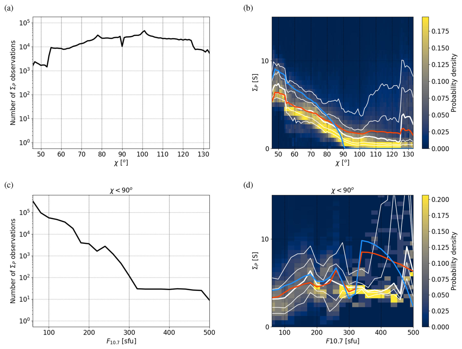
Figure 1 Number of EISCAT observations of the Pedersen conductance Σ_P as a function of the solar zenith angle χ (a) and distribution of the observed Σ_P (b). For the distribution, the sum of values in each column is 1. The thick white curve is the median and the thin white curves are the 10, 25, 75, and 90 percentiles. The red curve is the median calculated using our new model, including both EUV and precipitation components, and the blue curve is the median calculated using the Moen and Brekke (1993) empirical model (Eq. 29). The bottom row shows corresponding data with χ<90° as a function F_10.7.

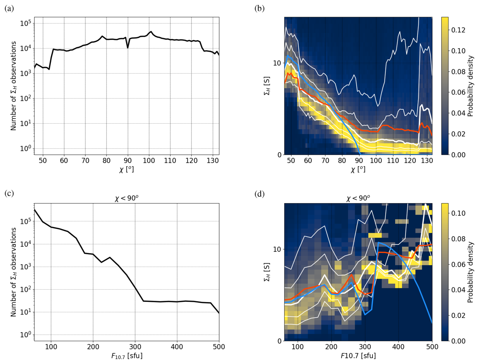
Figure 2 The same as Fig. 1 except for the Hall conductance Σ_H instead of the Pedersen conductance Σ_P.

Ahn et al. (1998) used Chatanika radar data to derive an empirical model for Σ_precip as a function of horizontal (ΔH) and vertical (ΔZ) ground magnetic field perturbations and magnetic local time (MLT). They used a relationship of the form

$$\begin{array}{}\text{(32)}& \mathrm{\Sigma }=\left\{\begin{array}{ll}{a}_{\mathrm{1}}\left(\text{MLT}\right)|\mathrm{\Delta }H{|}^{a_{\mathrm{2}}\left(\text{MLT}\right)},& \mathrm{\Delta }H<\mathrm{0},\mathrm{\Delta }Z<\mathrm{0}\\ a_{\mathrm{3}}\left(\text{MLT}\right)|\mathrm{\Delta }H{|}^{a_{\mathrm{4}}\left(\text{MLT}\right)},& \mathrm{\Delta }H<\mathrm{0},\mathrm{\Delta }Z>\mathrm{0}\\ a_{\mathrm{5}}\left(\text{MLT}\right)|\mathrm{\Delta }H{|}^{a_{\mathrm{6}}\left(\text{MLT}\right)},& \mathrm{\Delta }H>\mathrm{0},\mathrm{\Delta }Z<\mathrm{0}\\ a_{\mathrm{7}}\left(\text{MLT}\right)|\mathrm{\Delta }H{|}^{a_{\mathrm{8}}\left(\text{MLT}\right)},& \mathrm{\Delta }H>\mathrm{0},\mathrm{\Delta }Z>\mathrm{0}\end{array}\right.,\end{array}$$

where the coefficients a(MLT) for different MLT sectors were determined by fitting the model to the observations. For the eastward electrojet region, the sectors were 13:00–15:00, 16:00–18:00, 19:00–21:00, 22:00–23:00, and 00:00–02:00 MLT and for the westward electrojet region, 19:00–21:00, 22:00–23:00, 00:00–02:00, 03:00–04:00, 05:00–06:00, 07:00–09:00, and 10:00–12:00 MLT.

We choose a similar approach, except that instead of $\left|\mathrm{\Delta }H\right|$ we use $\left|{\mathit{J}}_{\text{DF}}\right|$. We use $\left|{\mathit{J}}_{\text{DF}}\right|$ instead of J_eastward, which would correspond to ΔH, in order to avoid unphysical conductance structures when there is a J_DF pattern more complicated than a basic electrojet. (∇×J_DF)_r can be used as a proxy for the field-aligned current density under some conditions (see, e.g., Weygand and Wing, 2016; Juusola et al., 2023b), and higher conductance values might be expected for regions of upward field-aligned current than for downward field-aligned current. We tested using (∇×J_DF)_r in a similar way as Ahn et al. (1998) used ΔZ, but better results were obtained using $\left|{\mathit{J}}_{\text{DF}}\right|$ alone. Separate modelling of regions with positive and negative (∇×J_DF)_r tended to give higher conductances for the region of negative (∇×J_DF)_r, although opposite behavior is expected. The reason may be the limitation of (∇×J_DF)_r for describing the location of possible conductance gradients.

Figure 3 shows Σ_P as a function of $\left|{\mathit{J}}_{\text{DF}}\right|$, (∇×J_DF)_r, and MLT in a format similar to Fig. 1. Similar plots for Σ_H are displayed in Fig. 4. For our model, we use the expression

$$\begin{array}{}\text{(33)}& {\mathrm{\Sigma }}_{\text{precip}}=c_{\mathrm{4}}\left(\text{MLT}\right)|{\mathit{J}}_{\text{DF}}{|}^{c_{\mathrm{5}}\left(\text{MLT}\right)}.\end{array}$$

Unlike Ahn et al. (1998), we do not try to distinguish between the eastward and westward electrojet region, because such a separation is not always unambiguous, e.g., when the current has a strong north–south component. The MLT dependence of the coefficients c₄ and c₅ will describe the different regions to some extent. The asymmetric distribution of the number of conductance observations for positive and negative (∇×J_DF)_r in Figs. 3c and 4c may be related to the concentration of upward field-aligned current regions and the spreading of downward field-aligned current regions, as discussed for example by Yoshikawa et al. (2011).

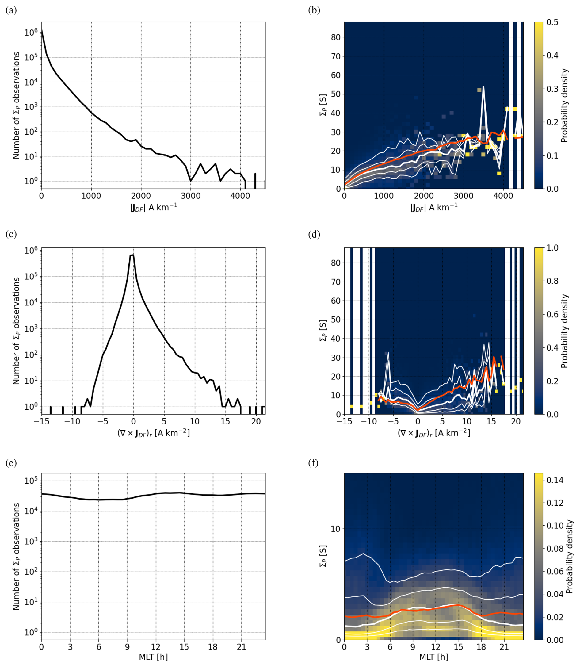
Figure 3 Σ_P as a function of $\left|{\mathit{J}}_{\text{DF}}\right|$, (∇×J_DF)_r, and MLT in a format similar to Fig. 1. Whenever there is no conductance data for a given value on the x axis, the corresponding distribution is replaced by a white bar.

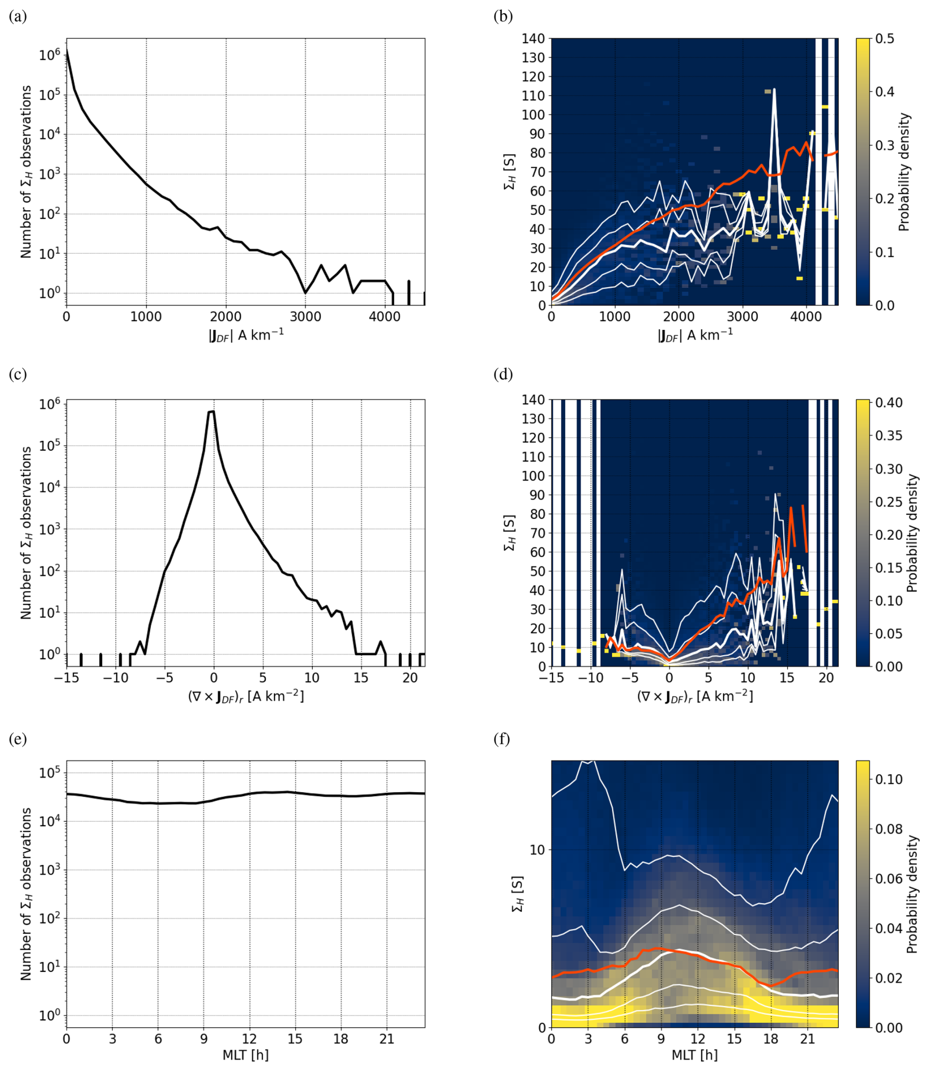
Figure 4 The same as Fig. 3 except for the Hall conductance Σ_H instead of the Pedersen conductance Σ_P.

The coefficients c₀–c₅, where c₀=Σ_BG is the constant background conductance, were determined by a least squares fit of the model to the observed Σ_P and Σ_H. The resulting values and standard deviation (STD) errors are provided in Tables 1–2. Linear interpolation was used for MLTs between those given in Table 2. The MLT-dependent coefficients c₄–c₅ are also illustrated in Fig. 5. The coefficient pair c₄ and c₅ describe the precipitation dependence of Σ_P and Σ_H. In Fig. 5, both pairs display a general systematic tendency for the other coefficient to strengthen as the other weakens. Larger values of c₅ indicate stronger dependence on $\left|{\mathit{J}}_{\text{DF}}\right|$. Close to noon, the coefficient c₅ is almost zero, which means that the conductance is almost independent of $\left|{\mathit{J}}_{\text{DF}}\right|$. The conductance is also clearly larger than the background level (c₄>c₀). This is not caused by photoionisation, because it is included in the model. So, it seems that there must be precipitation that enhances the E region electron density but is not visible in $\left|{\mathit{J}}_{\text{DF}}\right|$. A possible explanation are small-scale current systems that are not detected by ground-based magnetometers.

Table 1 Fitted values of the coefficients c₀–c₃ and their standard deviation (STD) errors from Eq. (31) ([F_10.7]=sfu, [Σ_EUV]=S) and from Σ_BG=c₀ ([Σ_BG]=S) for Σ_P and Σ_H.

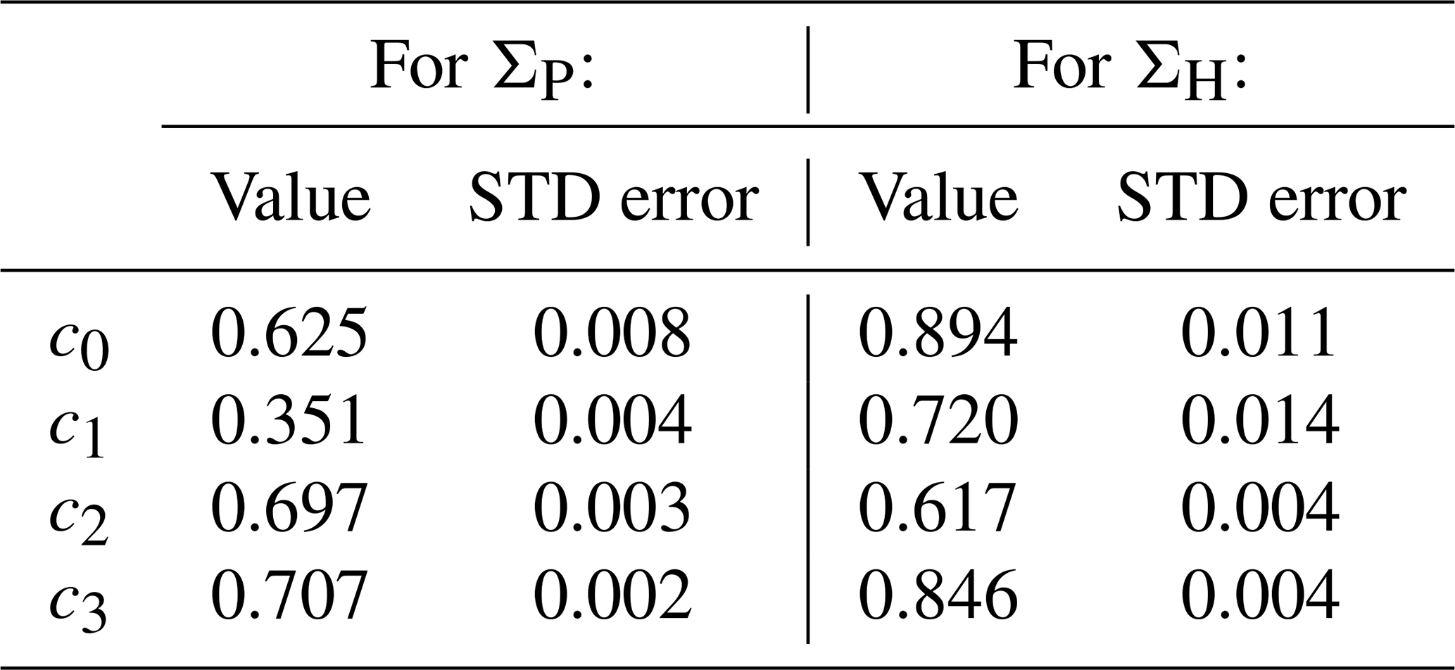
Table 2 Fitted values of the MLT dependent coefficients c₄ and c₅ and their standard deviation (STD) errors from Eq. (33) ($\left[\right|{\mathit{J}}_{\text{DF}}\left|\right]=\mathrm{A}/\mathrm{km}$, [Σ_precip]=S) for Σ_P and Σ_H.

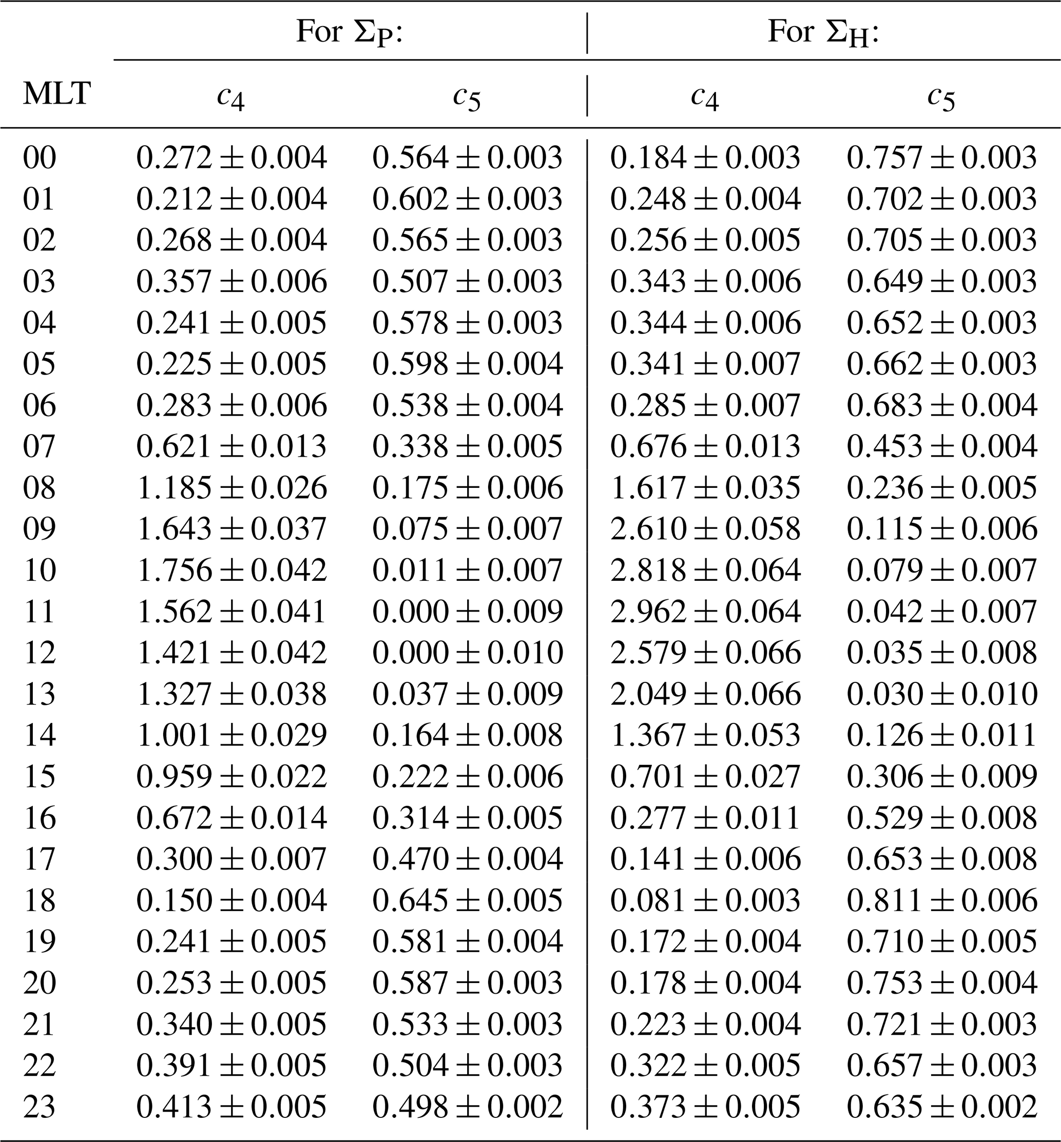
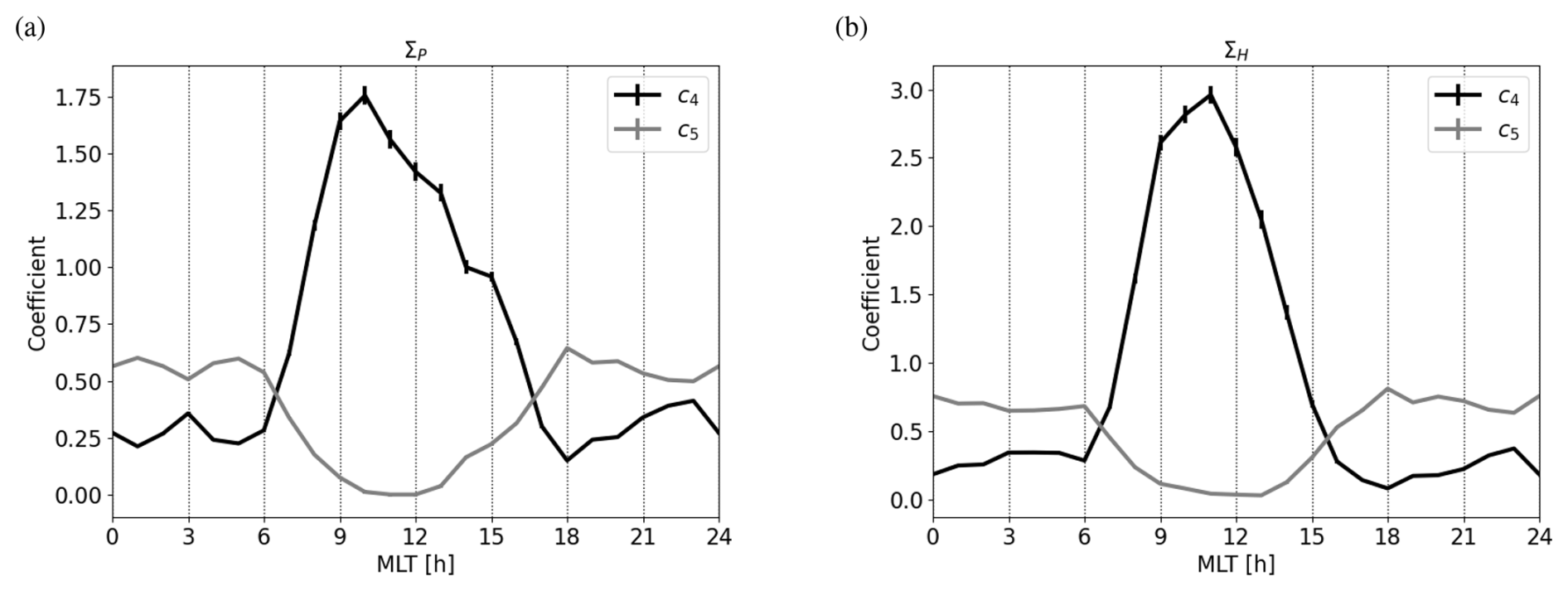
Figure 5 Coefficients c₄ and c₅ from Eq. (33) as a function of MLT for Σ_P (a) and Σ_H (b). Standard deviation errors of the coefficients are indicated by vertical line segments.

The correlation coefficient between the observed and modelled data is CC=0.66 for both Σ_P and Σ_H. The coefficient of determination

$$\begin{array}{}\text{(34)}& R^{\mathrm{2}}=\mathrm{1}-{\displaystyle \frac{{\sum }_i({\mathrm{\Sigma }}_i^{\text{obs}}-{\mathrm{\Sigma }}_i^{\text{mod}}{)}^{\mathrm{2}}}{{\sum }_i({\mathrm{\Sigma }}_i^{\text{obs}}-\text{mean}({\mathrm{\Sigma }}^{\text{obs}}){)}^{\mathrm{2}}}}\end{array}$$

is R²=0.43 for Σ_P and R²=0.44 for Σ_H. Considering that the scale sizes of IMAGE-based J_DF and EISCAT-based conductances are different, meso-scale and small-scale, respectively, these numbers seem reasonable. The thick white and red curves in Figs. 1–4 show the median of the observed and modelled values, respectively. Generally, the white and red curves follow each other relatively well, and in Figs. 1b and 2b, the red curves fit the data better than the Moen and Brekke (1993) model (blue curves). The wrong dependence on (∇×J_DF)_r, discussed above, is also visible in the median curves of the observed and modelled data in Figs. 3d and 4d.

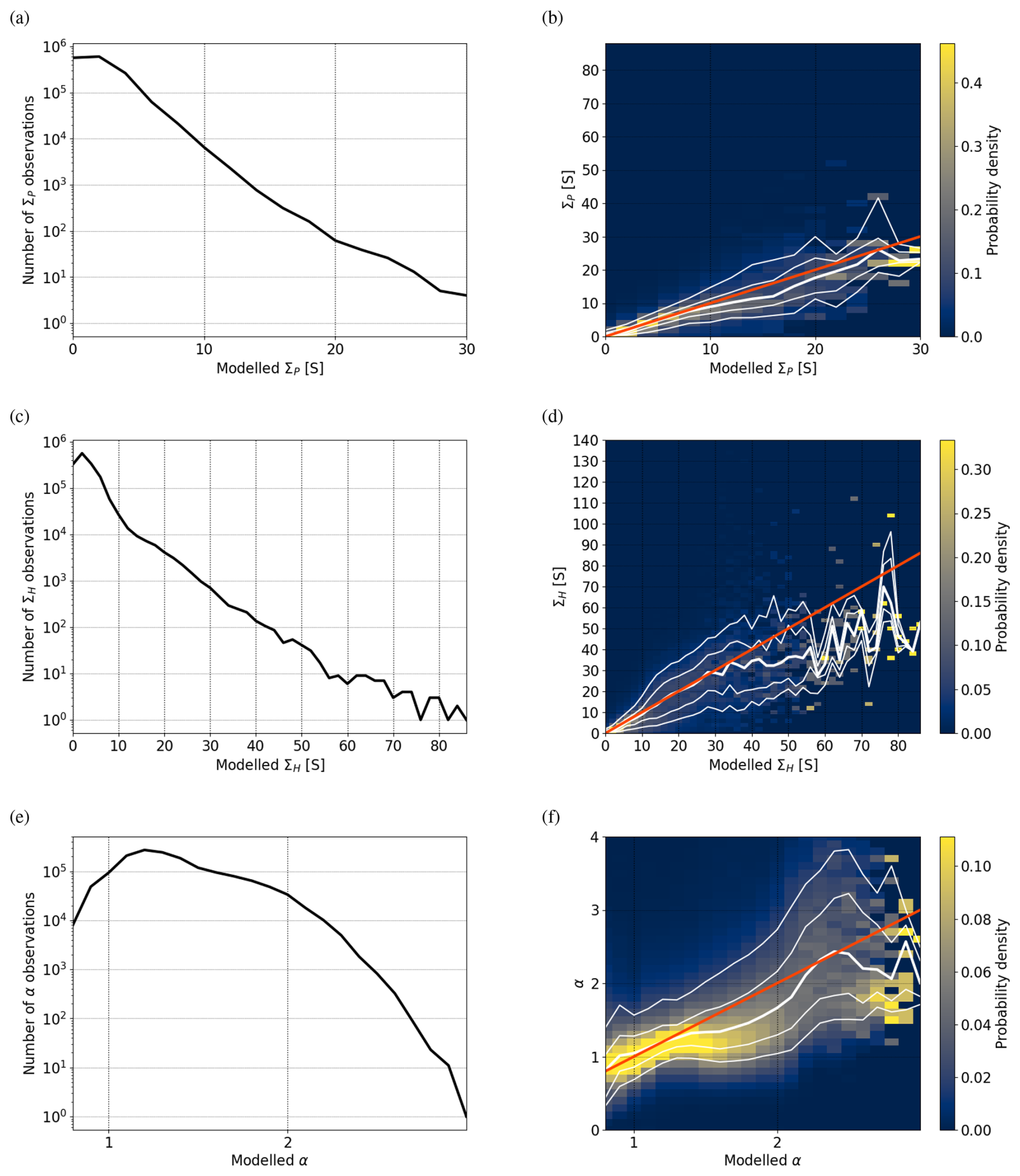
Figure 6 shows the observed Σ_P (top), Σ_H (middle), and Hall-to-Pedersen conductance ratio $\mathit{\alpha }=\frac{{\mathrm{\Sigma }}_{\mathrm{H}}}{{\mathrm{\Sigma }}_{\mathrm{P}}}$ (bottom) as a function of the modelled value in a format similar to Figs. 1–4. The red curves in the right column are lines of unity. The median curve aligns well with the line of unity for all three parameters, indicating good agreement between observed and modelled values.

Figure 6 Observed Σ_P (a, b) Σ_H (c, d), and Hall-to-Pedersen conductance ratio $\mathit{\alpha }=\frac{{\mathrm{\Sigma }}_{\mathrm{H}}}{{\mathrm{\Sigma }}_{\mathrm{P}}}$ (e, f) as a function of the modelled value in a format similar to Figs. 1–4. The red line is the line of unity.

A summary of fitting the model is displayed on the left hand side of Fig. 7. The right hand side illustrates how the model is used in Sects. 3.2 (“Option a”) and 3.3 (“Option b”). We will call the new model “Ebec” for EISCAT-based empirical conductance model.

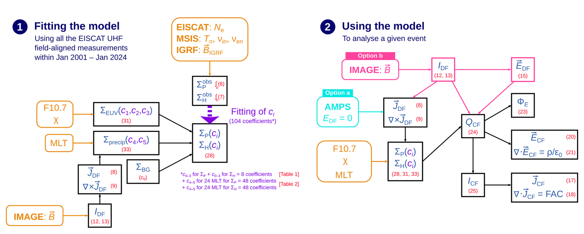
Figure 7 Summary of fitting the Ebec model (1) and using the Ebec model (2). Input data are in yellow, derived parameters in blue, model coefficients in purple, and equation numbers in red. The right hand side illustrates how the model is used in Sects. 3.2 (“Option a”, cyan color) and 3.3 (“Option b”, pink color).

3.2 Comparison with the SWIPE model

In order to start validating the new empirical conductance model, we will apply it to $\left|{\mathit{J}}_{\text{DF}}\right|$ from the Average Magnetic field and Polar current System (AMPS) model (Laundal et al., 2018) and compare with the Swarm Ionospheric Polar Electrodynamics (SWIPE) model (Hatch et al., 2024) conductances for the same conditions. AMPS is a climatological model of polar ionospheric currents, based on magnetic field measurements from the CHAMP and Swarm satellites, and SWIPE is a climatological model of polar ionospheric electrodynamics, based on the Thermal Ion Imager (TII) and Vector Field Magnetometer (VFM) instruments carried by Swarm. Both AMPS and SWIPE are parametrized with magnetic latitude, MLT, dipole tilt angle, solar wind speed, F_10.7, and Interplanetary Magnetic Field (IMF) B_GSM,y and B_GSM,z. AMPS provides the DF and CF part of the horizontal ionospheric current density and the field-aligned current density. SWIPE provides the ionospheric Hall and Pedersen conductances and horizontal potential electric field and corresponding potential. E_DF is assumed to be zero.

Because SWIPE has not been very extensively validated, we will first compare the SWIPE conductances with EISCAT observations. Figure 8 is otherwise the same as Fig. 6a–d except that instead of the new EISCAT-based model, values modelled using SWIPE are compared with the EISCAT observations. The solar wind speed and interplanetary magnetic field data propagated to Earth's bow shock nose that were needed as input for SWIPE were extracted from NASA/GSFC's OMNI data set through OMNIWeb (Papitashvili and King, 2020). We have not included SWIPE conductances that should be masked according to the criteria specified in Hatch et al. (2024) ($\mathit{J}\cdot \mathit{E}<\mathrm{0.5}\mathrm{mW}{\mathrm{m}}^{-\mathrm{2}}$; Σ≤0 S). Figure 8 shows that there is reasonable agreement between SWIPE and EISCAT for small conductance values.

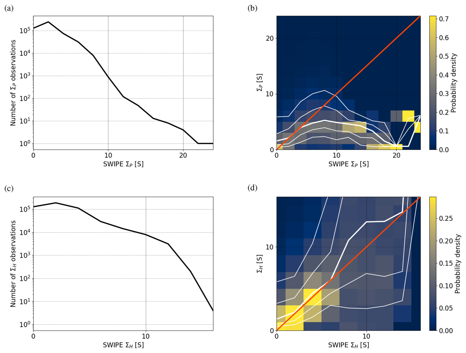
Figure 8 The same as Fig. 6a–d except that instead of Ebec, values modelled using SWIPE are compared with the EISCAT observations.

Figure 9a shows $\left|{\mathit{J}}_{\text{DF}}\right|$ from AMPS as a function of magnetic latitude and MLT for dipole tilt angle 0° (equinox), solar wind speed V=450 km s⁻¹, F_10.7=120 sfu, IMF $B_{\text{GSM},y}=\mathrm{0}$ nT and $B_{\text{GSM},z}=-\mathrm{5}$ nT. For reference, we also show contours of the field-aligned current density from AMPS. Figure 9b and 9c show the conductances estimated using our model, and 9d and 9e show the conductances from the SWIPE model for the same conditions as those applied to the AMPS model. There are some white areas in the modelled conductances, because SWIPE can only produce conductance estimates when the conductances are “electrodynamically visible”. That is, if J and E are not large enough or if $\mathit{J}\cdot \mathit{E}<\mathrm{0}$, the conductances cannot be estimated. As a result, SWIPE conductances have a baseline uncertainty of at least 0.5 S (Hatch et al., 2024).

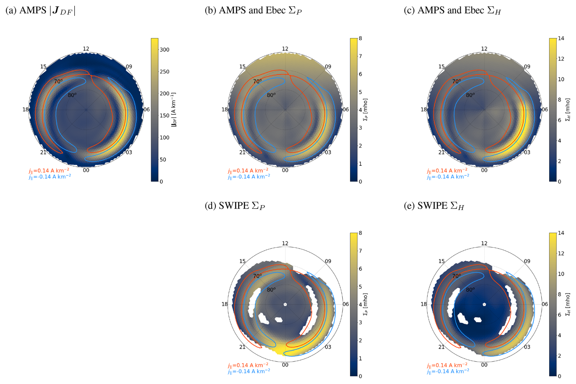
Figure 9 (a) $\left|{\mathit{J}}_{\text{DF}}\right|$ as a function of magnetic latitude and MLT according to the AMPS model (Laundal et al., 2018) for dipole tilt angle 0° (equinox), solar wind speed V=450 km s⁻¹, F_10.7=120 sfu, IMF $B_{\text{GSM},y}=\mathrm{0}$ nT and $B_{\text{GSM},z}=-\mathrm{5}$ nT. The contours indicate regions of upward (blue) and downward (red) field-aligned current density according to AMPS. (b) Σ_P according to the EISCAT-based empirical model Ebec for the AMPS J_DF. (c) Σ_H according to Ebec for the AMPS J_DF. (d) Σ_P according to the SWIPE model (Hatch et al., 2024) for the same conditions as AMPS. (e) Σ_H according to the SWIPE model. The red and blue contours are the same in all panels.

Both SWIPE and Ebec conductances show the highest values in the midnight and morning sector auroral oval. For SWIPE, the maximum of Σ_P is around midnight and of Σ_H around 3 MLT, whereas for Ebec the entire post-midnight sector shows increased values. The maximum amplitude of Ebec Σ_H (15 S) is somewhat higher than that of SWIPE (12 S) whereas the maximum amplitude of Ebec Σ_P (7 S) is slightly lower than that of SWIPE (9 S).

Next, we solve Eq. (24) for Q_CF,i using Σ_P from Fig. 9b, Σ_H from Fig. 9c, and I_DF,i from AMPS (∇×J_DF)_r according to Eq. (9). AMPS (∇×J_DF)_r is shown in Fig. 10a. The red and blue field-aligned current density contours in Fig. 10a are based on AMPS data and identical to those in Fig. 9. E_DF is assumed to be negligible. I_CF is then determined using Eq. (25). We have used a triangular grid and only included triangles where all nodes have latitudes ≥60°. The values of $\left|{\mathit{J}}_{\text{DF}}\right|$, (∇×J_DF)_r, Σ_P, and Σ_H were first calculated for the grid nodes. The conductance gradients and values for the triangle faces were estimating using the finite difference approach

$$\begin{array}{ll}\text{(35)}& {\displaystyle }\mathrm{\nabla }{\mathrm{\Sigma }}_{\mathit{\theta },\text{face}}=& {\displaystyle \frac{{\mathrm{\Sigma }}_{\text{node2}}-{\mathrm{\Sigma }}_{\text{node1}}}{R({\mathit{\theta }}_{\text{node2}}-{\mathit{\theta }}_{\text{node1}})}}\text{(36)}& {\displaystyle }\mathrm{\nabla }{\mathrm{\Sigma }}_{\mathit{\varphi },\text{face}}=& {\displaystyle \frac{{\mathrm{\Sigma }}_{\text{node2}}-{\mathrm{\Sigma }}_{\text{node1}}}{R\sin {\mathit{\theta }}_{\text{face}}({\mathit{\varphi }}_{\text{node2}}-{\mathit{\varphi }}_{\text{node1}})}}\text{(37)}& {\displaystyle }{\mathrm{\Sigma }}_{\text{face}}=& {\displaystyle \frac{{\mathrm{\Sigma }}_{\text{node1}}+{\mathrm{\Sigma }}_{\text{node2}}+{\mathrm{\Sigma }}_{\text{node3}}}{\mathrm{3}}}{\displaystyle }{A}_{\text{face}}=& {\displaystyle }{R}^{\mathrm{2}}\cdot (C_{\text{node1,node2}}+C_{\text{node2,node3}}\\ \text{(38)}& {\displaystyle }& {\displaystyle }+C_{\text{node3,node1}}-\mathit{\pi }),\end{array}$$

where the triangle cell area A in Eqs. (24) and (25) was calculated from the excess of the triangle angles C. The two out of three nodes used to calculate the gradients were selected to yield the largest latitude and longitude variations across the triangle. The face grid was used to solve Eqs. (24) and (25). The resulting field-aligned current density and electric potential are displayed in Fig. 10b and c. The corresponding distributions from AMPS and SWIPE are illustrated in Fig. 10d and e.

AMPS (Fig. 10d) shows the expected pattern of Region 1 and Region 2 field-aligned current rings. In the dusk sector, the pattern and amplitudes produced by the combination of AMPS and Ebec (Fig. 10b) are quite similar. In the dawn sector, the direction of the field-aligned current density more or less agrees with AMPS, but the amplitude is clearly weaker. SWIPE (Fig. 10e) shows the expected two-cell convection pattern with a potential difference of 93 kV. AMPS+Ebec (Fig. 10c) also produces a two-cell convection pattern, but the potential drop is smaller, 77 kV. The difference can be explained by the higher Hall conductance of the Ebec model (Fig. 9c) compared to the SWIPE model (Fig. 9e).

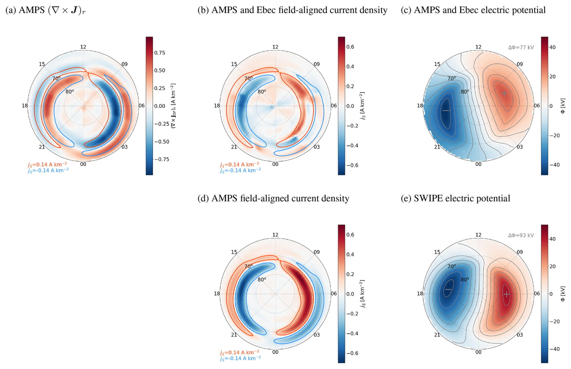
Figure 10 (a) (∇×J)_r as a function of magnetic latitude and MLT according to the AMPS model (Laundal et al., 2018) for the same model parameters as Fig. 9. (b, c) Field-aligned current density and electric potential solved using Eqs. (24) and (25) and the distributions in Figs. 9a–c and 10a. E_DF is assumed to be negligible. (d) Field-aligned current density according to the AMPS model. The contours indicate regions of upward (blue) and downward (red) field-aligned current density with amplitude exceeding 0.14 A km⁻². (e) Electric potential according to the SWIPE model (Hatch et al., 2024). The red and blue contours in (a) and (b) are identical to those in panel (d).

3.3 Combining IMAGE observations and the empirical conductance model

In this section, we will apply the new empirical conductance model to solve Eq. (24) for Q_CF,i when I_DF,i and E_DF have been determined by applying the 2D SECS method to IMAGE magnetic field observations. I_CF is then determined using Eq. (25). First, we determine Σ_P and Σ_H from the known J_DF, F_10.7, χ, and MLT, as described in Sect. 3.1. The conductance gradients and conductances at the same locations are then estimated using the finite difference approach,

$$\begin{array}{}\text{(39)}& {\displaystyle }\begin{array}{rl}{\displaystyle }\mathrm{\nabla }{\mathrm{\Sigma }}_{\mathit{\theta },i+\frac{\mathrm{1}}{\mathrm{2}},j+\frac{\mathrm{1}}{\mathrm{2}}}=& {\displaystyle \frac{\mathrm{1}}{\mathrm{2}}}\cdot \left({\displaystyle \frac{{\mathrm{\Sigma }}_{i+\mathrm{1},j}-{\mathrm{\Sigma }}_{i,j}}{R\mathrm{\Delta }\mathit{\theta }}}\right.\\ {\displaystyle }& {\displaystyle }\left.+{\displaystyle \frac{{\mathrm{\Sigma }}_{i+\mathrm{1},j+\mathrm{1}}-{\mathrm{\Sigma }}_{i,j+\mathrm{1}}}{R\mathrm{\Delta }\mathit{\theta }}}\right)\end{array}\text{(40)}& {\displaystyle }\begin{array}{rl}{\displaystyle }\mathrm{\nabla }{\mathrm{\Sigma }}_{\mathit{\varphi },i+\frac{\mathrm{1}}{\mathrm{2}},j+\frac{\mathrm{1}}{\mathrm{2}}}=& {\displaystyle \frac{\mathrm{1}}{\mathrm{2}}}\cdot \left({\displaystyle \frac{{\mathrm{\Sigma }}_{i,j+\mathrm{1}}-{\mathrm{\Sigma }}_{i,j}}{R\sin {\mathit{\theta }}_{\mathit{\varphi },i+\frac{\mathrm{1}}{\mathrm{2}},j+\frac{\mathrm{1}}{\mathrm{2}}}\mathrm{\Delta }\mathit{\varphi }}}\right.\\ {\displaystyle }& {\displaystyle }\left.+{\displaystyle \frac{{\mathrm{\Sigma }}_{i+\mathrm{1},j+\mathrm{1}}-{\mathrm{\Sigma }}_{i+\mathrm{1},j}}{R\sin {\mathit{\theta }}_{\mathit{\varphi },i+\frac{\mathrm{1}}{\mathrm{2}},j+\frac{\mathrm{1}}{\mathrm{2}}}\mathrm{\Delta }\mathit{\varphi }}}\right)\end{array}\text{(41)}& {\displaystyle }{\mathrm{\Sigma }}_{i+\frac{\mathrm{1}}{\mathrm{2}},j+\frac{\mathrm{1}}{\mathrm{2}}}={\displaystyle \frac{{\mathrm{\Sigma }}_{i,j}+{\mathrm{\Sigma }}_{i+\mathrm{1},j}+{\mathrm{\Sigma }}_{i,j+\mathrm{1}}+{\mathrm{\Sigma }}_{i+\mathrm{1},j+\mathrm{1}}}{\mathrm{4}}}\text{(42)}& {\displaystyle }{A}_{i+\frac{\mathrm{1}}{\mathrm{2}},j+\frac{\mathrm{1}}{\mathrm{2}}}=\mathrm{2}{R}^{\mathrm{2}}\mathrm{\Delta }\mathit{\varphi }\sin {\mathit{\theta }}_{i+\frac{\mathrm{1}}{\mathrm{2}},j+\frac{\mathrm{1}}{\mathrm{2}}}\sin {\displaystyle \frac{\mathrm{\Delta }\mathit{\theta }}{\mathrm{2}}}.\end{array}$$

Here, A is the grid cell area in Eqs. (24) and (25), Δθ is the co-latitude grid resolution, and Δϕ is the longitude grid resolution for the rectangular grid.

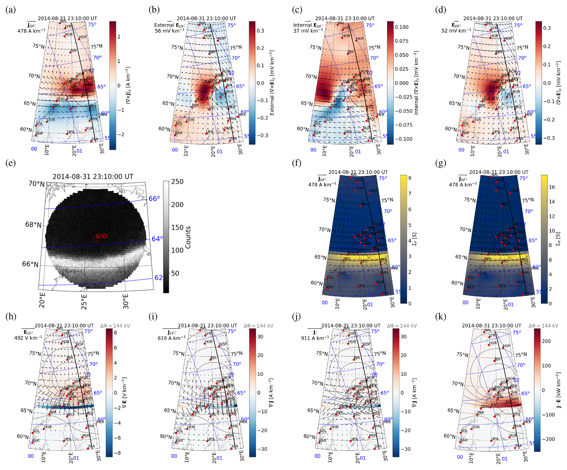
Figure 11 shows an example of the application of the 2D SECS method to IMAGE magnetic field data. Figure 11a displays J_DF (arrows) and $(\mathrm{\nabla }\times {\mathit{J}}_{\text{DF}}{)}_z=-(\mathrm{\nabla }\times {\mathit{J}}_{\text{DF}}{)}_{\mathrm{r}}$ (color) as a function of geographic latitude and longitude on 31 August 2014 at 23:10:00 UT (Juusola et al., 2016a). Locations of the IMAGE stations used in the analysis are indicated by the red circles and Apex coordinates (Richmond, 1995; Emmert et al., 2010; Laundal et al., 2022b) with the blue grid. The event took place in the post-midnight sector, around 01 MLT. The SOD all-sky camera field-of-view is indicated by the black circle and the track of Swarm A by the black line. J_DF shows a westward electrojet. Figure 11b illustrates the external part of E_DF due to time-varying ionospheric currents, Fig. 11c internal part of E_DF due to time-varying telluric currents (Juusola et al., 2025b), and Fig. 11d the total E_DF. E_DF is displayed by the vectors and (∇×E_DF)_z by the color. The values are small due to the stationarity of the event.

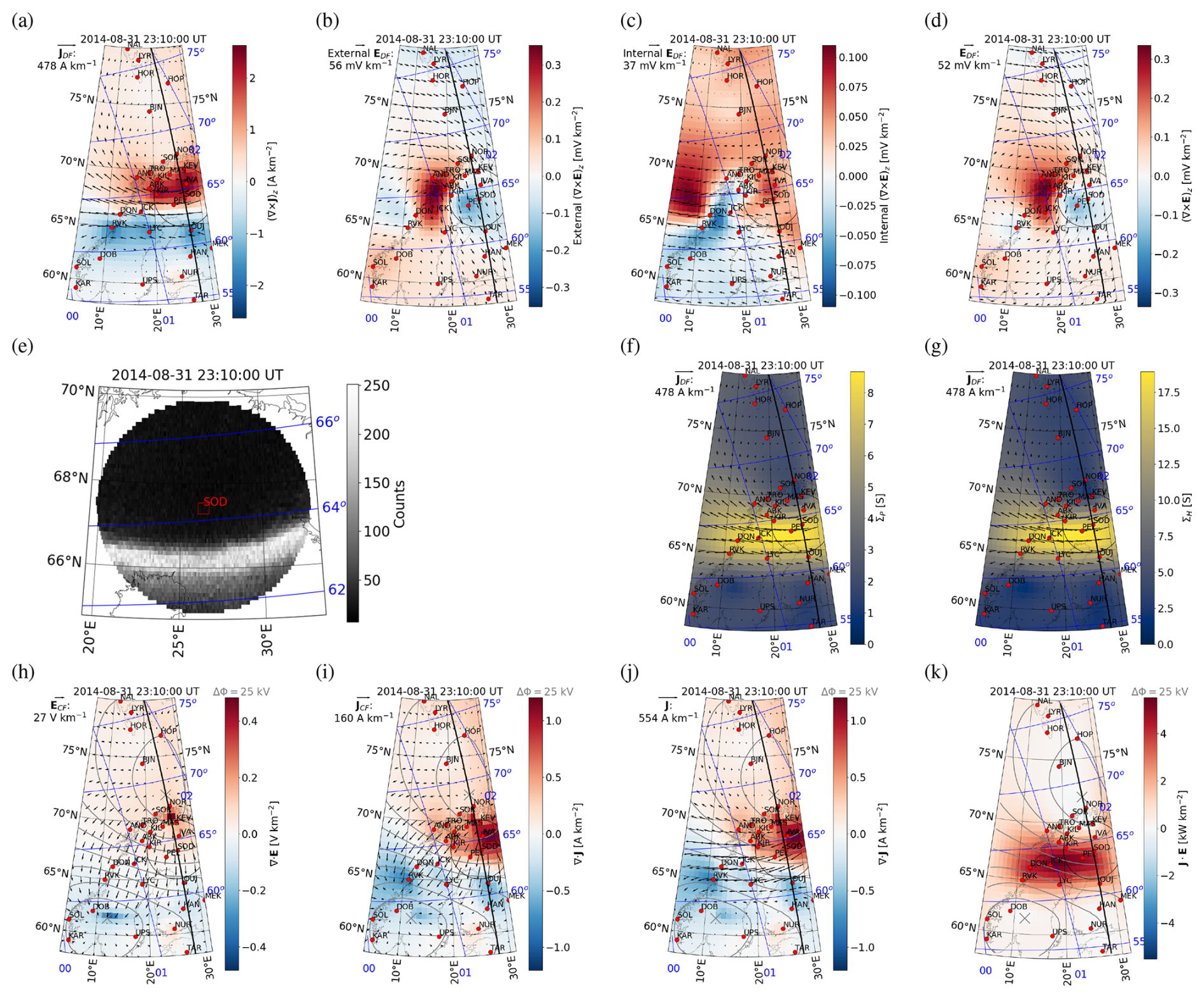
Figure 11 Morning sector auroral arc event on 31 August 2014 at 23:10:00 UT. (a) Divergence-free part of the ionospheric horizontal current density (external J_DF, arrows) and its curl ($(\mathrm{\nabla }\times {\mathit{J}}_{\text{DF}}{)}_z=-(\mathrm{\nabla }\times {\mathit{J}}_{\text{DF}}{)}_{\mathrm{r}}$, color) as a function of geographic latitude and longitude, derived from IMAGE magnetometer data. Locations of the IMAGE stations used in the analysis are indicated by the red circles, apex coordinates (Richmond, 1995; Emmert et al., 2010; Laundal et al., 2022b) with the blue grid, the SOD all-sky camera field-of-view by the black circle, and the track of the Swarm A satellite by the black line. (b–d) External part, internal part, and total ionospheric divergence-free electric field (E_DF, arrows) and its curl ((∇×E_DF)_z, color). (e) Auroral intensity from the SOD all-sky camera mapped to 110 km altitude. (f, g) Pedersen conductance (Σ_P, color) and Hall conductance (Σ_H, color) according to the Ebec model for J_DF (arrows). (h) Curl-free horizontal ionospheric electric field (E_CF, arrows) and its divergence (∇⋅E_CF, color). (i) Curl-free horizontal ionospheric current density (J_CF, arrows) and its divergence ($\mathrm{\nabla }\cdot {\mathit{J}}_{\text{CF}}=j_z=-j_{\mathrm{r}}$, color). (j) Total horizontal ionospheric current density ($\mathit{J}={\mathit{J}}_{\text{DF}}+{\mathit{J}}_{\text{CF}}$, arrows) and its divergence ($\mathrm{\nabla }\cdot \mathit{J}=j_z=-j_{\mathrm{r}}$, color). (k) Dot product between the total horizontal current density and electric field (J⋅E). The gray contours show the electric potential Φ. The maximum potential difference ΔΦ between the locations indicated by the gray crosses is given in the top left corner.

Figure 11e shows the auroral intensity from the SOD all-sky camera mapped to 110 km altitude. There is an auroral arc between 66.0° and 66.5° latitude, in the middle of the westward electrojet. The arrows in Fig. 11f–g repeat J_DF, and the color shows Σ_P and Σ_H estimated from J_DF and MLT. This is a nightside event for which Σ_EUV=0.

Figure 11h displays E_CF (arrows) and its divergence (∇⋅E_CF, color), Fig. 11i J_CF (arrows) and its divergence ($\mathrm{\nabla }\cdot {\mathit{J}}_{\text{CF}}=j_z=-j_{\mathrm{r}}$, color), Fig. 11j the total horizontal ionospheric current density ($\mathit{J}={\mathit{J}}_{\text{DF}}+{\mathit{J}}_{\text{CF}}$, arrows) and its divergence ($\mathrm{\nabla }\cdot \mathit{J}=j_z=-j_{\mathrm{r}}$, color), and Fig. 11k the dot product between the total horizontal current density and electric field (J⋅E) as a proxy for Joule heating. Any negative values of J⋅E indicate a dynamo. The gray curves illustrate contours of the electric potential (derived using Eq. 23), and the potential difference between the maximum and minimum, indicated by the gray crosses, is written in the top left corner of each panel.

There is upward current (negative ∇⋅J_CF in Fig. 11i) in the region where Fig. 11e shows the auroral arc and more diffuse emission south of the arc. North of the arc, in the region where there is no auroral emission, the field-aligned current is downward, as expected. The electric field in Fig. 11h is directed southward and maximizes north of the arc. This configuration of the field-aligned currents and electric field is typical for a morning sector auroral arc (e.g., Juusola et al., 2016a). J⋅E in Fig. 11k maximizes in the middle of the westward electrojet.

Similar plots for an evening sector auroral arc, observed by the KIL all-sky camera, are shown in Fig. 12. This time, the arc is located in the middle of an eastward electrojet. There is upward current (Fig. 12i) at the location of the arc (Fig. 12e), more diffuse downward current south of the arc, and an enhanced northward electric field (Fig. 12h) south of the arc, as expected for an evening sector auroral arc (Aikio et al., 2002). J⋅E in Fig. 12k maximizes in the middle of the eastward electrojet.

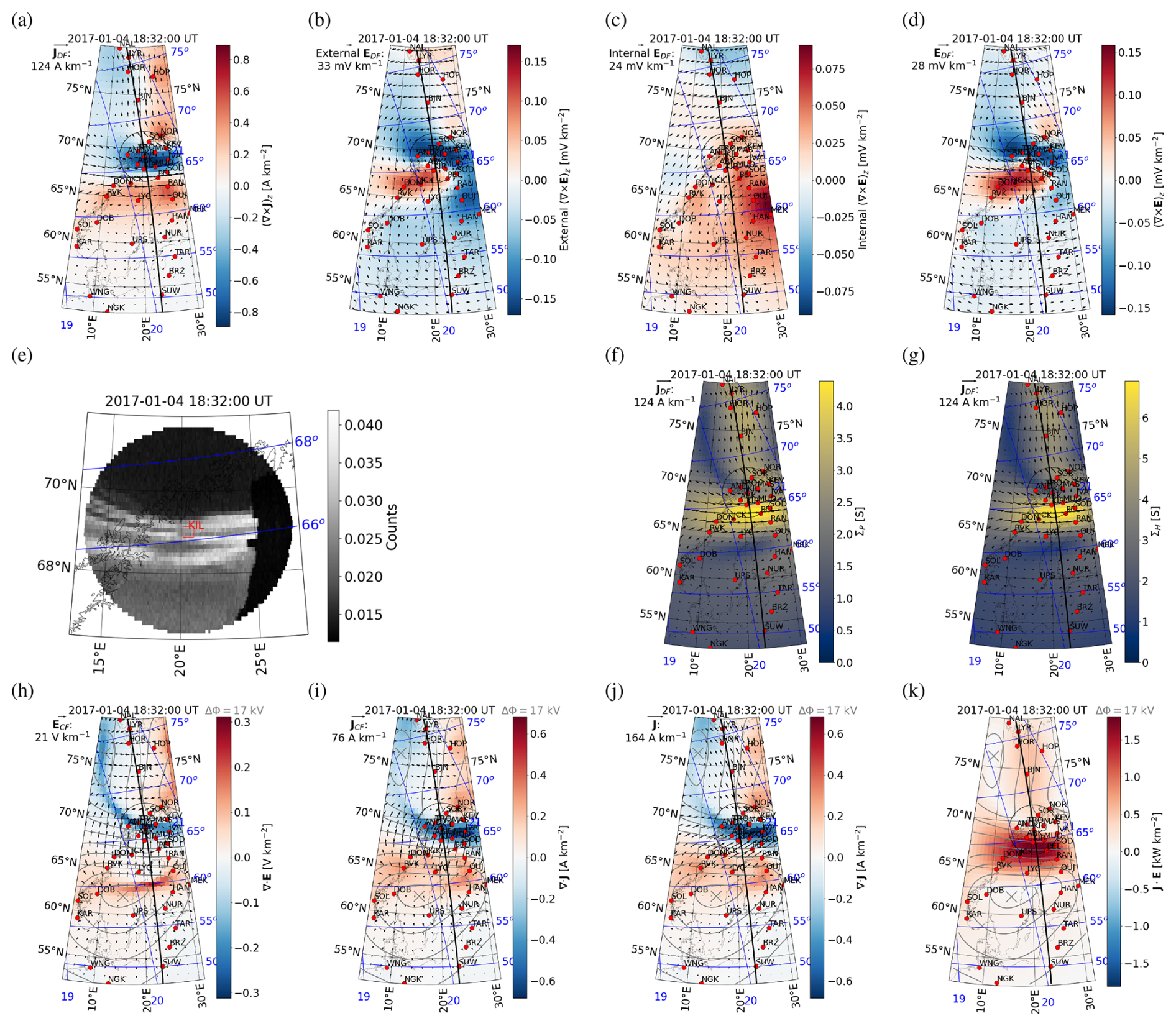
Figure 12 An evening sector auroral arc event on 4 January 2017 at 18:32:00 UT in the same format as Fig. 11. The all-sky camera is KIL instead of SOD.

3.4 Comparison with Swarm and AMPERE observations

In order to validate both the emprical model and the solver, we compare the electric field and radial current derived from IMAGE data to those observed by Swarm A and C satellites as they crossed IMAGE. The radial current is also compared to the large-scale radial current from AMPERE. The ten minute integration time required by AMPERE data analysis was selected to best agree with the time window of each Swarm crossing. Nearest neighbour interpolation was used to obtain AMPERE data at the footpoints of Swarm A.

Figure 13 illustrates four example crossings, including the two auroral arc crossings of the previous section. For each crossing, the three panels from top to bottom show the electric field as observed by Swarm A (black) and the electric field component parallel to the Swarm A track modelled based on IMAGE observations (red). The middle panel shows the single satellite radial current from Swarm A (black; scale on the left), dual satellite radial current from Swarm A and C (blue; scale on the right), radial current modelled based on IMAGE observations (red; scale on the right), and radial current from AMPERE (orange; scale on the right). The bottom panel shows the solar zenith angle χ (black; scale on the left) and MLT (blue; scale on the right). The F_10.7 flux value during the crossing is indicated in the bottom panel as well. The shaded region indicates a large gap in the IMAGE magnetometer latitude coverage. The grey curves in Fig. 13a and d will be discussed in Sect. 4.2.

The two crossings in the top row took place in darkness (χ>90°), such that Σ_EUV=0, and the two crossing in the bottom row took place in sunlight (χ<90°), such that Σ_EUV>0. In all four events, the IMAGE-based electric field estimate (red) has a reasonably similar profile as the large-scale Swarm observation, but the amplitude is weaker, especially for the post-midnight sector auroral oval crossings (Fig. 13a and d). There is a reasonable agreement on the direction of the large-scale radial current from Swarm A and C and IMAGE. The meso-scale radial currents from IMAGE have a somewhat better agreement with the larger-scale AMPERE currents than with the smaller-scale Swarm currents, highlighted the importance of spatial scales in the conductances and electrodynamic modeling results.

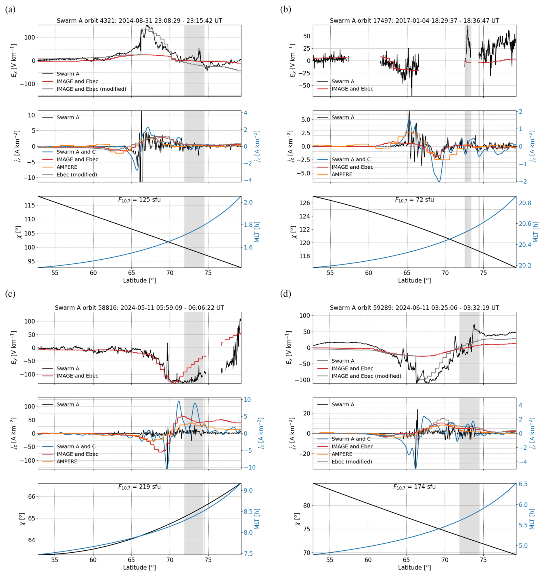
Figure 13 Four Swarm crossings of IMAGE (a–d). Top: Ionospheric electric field component corresponding to the ion drift measured by Swarm A perpendicular to the satellite orbit (black) and IMAGE+Ebec estimate of the same component (red). Middle: Radial current density estimated from Swarm A using the single satellite method (Ritter et al., 2013) (black, left scale), from the Swarm A and C satellite pair using the dual-satellite method (Ritter et al., 2013) (blue, right scale), from AMPERE using spherical harmonic fits (Waters et al., 2020) (orange, right scale), and the IMAGE+Ebec estimate (red, right scale). Bottom: Sun zenith angle χ (black; left scale) and MLT (blue, right scale). The gray curves in the top and middle panels of crossings (a) and (d) are otherwise the same as the red curves except that a modified conductance model (Sect. 4.2) is used.

3.5 Comparison with conductance models parametrized with field-aligned currents

Recent models by Robinson et al. (2020) and Wang and Zou (2022) correlate conductances from the Poker Flat Incoherent Scattering Radar (PFISR) with field-aligned currents from AMPERE and Swarm, respectively, thus ensuring the conductances and their gradients are self-consistent with the parallel currents. The latitudinal scale of AMPERE field-aligned currents is about 3° (Waters et al., 2020) and field-aligned current variations with a latitudinal scale of 150 km were used by Wang and Zou (2022). Thus, although the difference in spatial resolution between the EISCAT measurements and the equivalent currents derived from IMAGE magnetometers is a significant drawback to the Ebec model, the models parametrized by field-aligned currents also have similar limitations.

Figure 14 shows Σ_P and Σ_H as given by the conductance models of Robinson et al. (2020) and Wang and Zou (2022) when applied to the AMPS field-aligned current density (Fig. 10d). Note that due to the large differences in conductance amplitudes, the color scales are not the same as those in Fig. 9b–e. Apart from the amplitudes, the most obvious difference in the conductances given by Robinson et al. (2020) and Wang and Zou (2022) compared to SWIPE and Ebec is the latitudinally wide double oval structure caused by parametrizing by both upward and downward field-aligned current density. The coefficients of the COMPASS model by Wang and Zou (2022) are defined for three-hour MLT sectors, resulting in the discontinuous conductance distributions that could be smoothed, e.g., by interpolation.

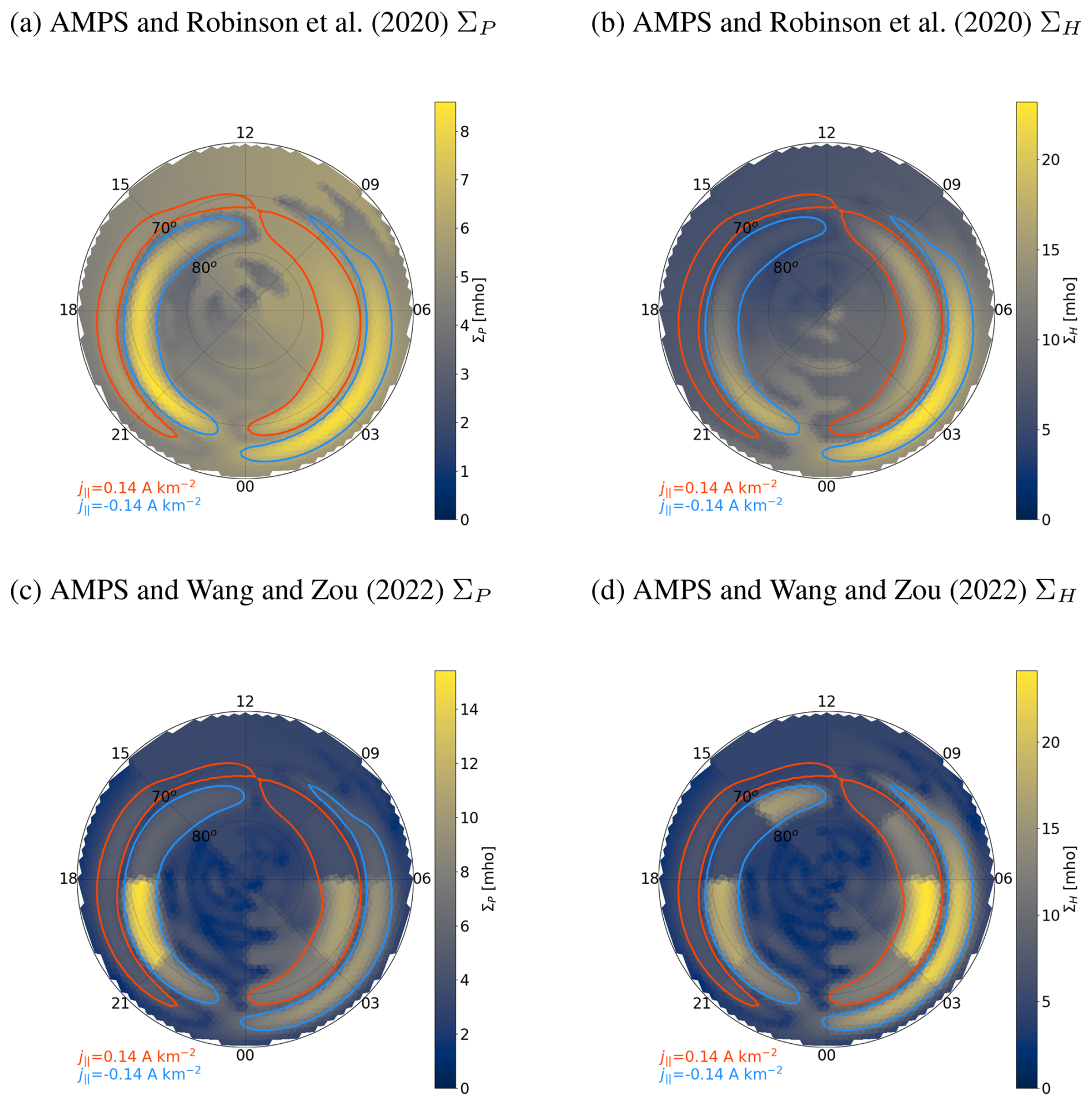
Figure 14 The same as Fig. 9b and c except for the Robinson et al. (2020) (a, b) and Wang and Zou (2022) (c, d) conductance models parametrized with AMPS field-aligned current density (Fig. 10d) instead of the Ebec model parametrized with AMPS $\left|{\mathit{J}}_{\text{DF}}\right|$ (Fig. 9a). Note that due to the large differences in conductance amplitudes the color scales are not the same as those in Fig. 9b–e.

4 Discussion

4.1 Limitations of the conductance model

The precipitation component of our conductance model is parametrized with the divergence-free component of the horizontal ionospheric current density. In addition to the auroral oval, $\left|{\mathit{J}}_{\text{DF}}\right|$ generally has a significant value in the polar cap as well. In the dark polar cap, J_DF and J_CF tend to oppose each other, summing up to almost zero (Laundal et al., 2018). Thus, while Σ_EUV is in principle expected to be valid everywhere, Σ_precip is not valid inside the polar cap. Examination of the global maps in Fig. 9 clearly shows that the values given by our model for the polar cap are too large. The model by Ahn et al. (1998) had the same limitation. They noted that conductances in the dark polar cap are very low, Σ_H<2.0 S and Σ_P<1.0 S (Fuller-Rowell and Evans, 1987), and not particularly sensitive to geomagnetic activity. Conductances in the sunlit polar cap, on the other hand, are dominated by Σ_EUV. Thus, an improvement to our model would be to try to identify the boundary between auroral oval and polar cap from J_DF and apply the fitted constant background values (c₀ in Table 1) to that region.

Our EISCAT data set contains observations not only from the auroral oval but from the polar cap and subauroral region as well. Our modeling assumes that $\left|{\mathit{J}}_{\text{DF}}\right|$ is zero outside the auroral oval, which is not true and introduces some error to the model. Furthmore, we assume that the conductances have similar profiles as the meso-scale $\left|{\mathit{J}}_{\text{DF}}\right|$. The meso-scale conductivity profiles derived from Swarm data by Juusola et al. (2016a) for a single event appear to be in agreement with this. However, the small-scale Σ_P profile deviates from the meso-scale $\left|{\mathit{J}}_{\text{DF}}\right|$. Ritter et al. (2004) have shown that small-scale field-aligned currents typically occur in the middle of the westward electrojet. It is possible that there should be corresponding small-scale structure in J_DF as well, but ground magnetometers or Swarm are not able to distinguish it. The same applies to the dayside, where our model predicts Σ_precip values that are clearly larger than the background level but almost independent of $\left|{\mathit{J}}_{\text{DF}}\right|$, as discussed in Sect. 3.1. The Electrojet Zeeman Imaging Explorer (EZIE) mission (e.g., Laundal et al., 2021; Yee et al., 2021b, a) can help to clarify this.

Neutral wind v_n perpendicular to the ionospheric background magnetic field B₀ generally needs to be considered in ionospheric electrodynamics (e.g., Hatch et al., 2024). For example, in a coordinate system where the neutral wind is not zero, Ohm's law (Eq. 3) becomes

$$\begin{array}{}\text{(43)}& \mathit{J}={\mathrm{\Sigma }}_{\mathrm{P}}(\mathit{E}+{\mathit{v}}_{\mathrm{n}}\times {\mathit{B}}_{\mathrm{0}})+{\mathrm{\Sigma }}_{\mathrm{H}}(\mathit{E}+{\mathit{v}}_{\mathrm{n}}\times {\mathit{B}}_{\mathrm{0}})\times {\widehat{\mathit{e}}}_{\mathrm{r}}.\end{array}$$

Neutral wind is not required to estimate the electron density N_e from EISCAT observations and, thus, to estimate the conductivities with Eqs. (6) and (7). The Ebec model is parametrized with electric current, which is independent on the frame of reference determined by the neutral wind. Thus, neutral wind is not expected to introduce errors to the conductances given by Ebec, and the electric field estimated from equivalent current density and Ebec conductances is given in the frame of reference where the neutral wind is zero.

4.2 Possible role of conductance gradients in the post-midnight sector

As demonstrated by Figs. 10 and 13, the electric field and field-aligned current density solved using the conductance model tend to be suppressed in the post-midnight sector where the conductances are high. Reducing the peak amplitudes of the conductances significantly, to the same level as in the pre-midnight section, would increase the electric field and field-aligned current density, but this does not agree with the observations. Another possibility is to introduce conductance gradients to the model. As mentioned in Sect. 3.1, fitting the conductance data set with separate coefficients for the regions of positive and negative (∇×J)_r failed. We speculated that this may have been due to the limitation of (∇×J)_r to describe the location of the conductance gradient.

We will test the effects of conductance gradients for the two postmidnight crossings shown in Fig. 13a and d. In both cases, Swarm observes a sharp electric field intensification at geographic latitude 66°. We artificially produce sharp conductance gradients at this location by multiplying Σ_precip poleward of 66° latitude by 0.2 (crossing in Fig. 13a) or 0.1 (crossing in Fig. 13d). The multipliers were selected to produce an electric field intensification visually matching that observed by Swarm. We tested using the sign change of (∇×J)_r instead of the 66° latitude threshold, but the resulting electric field intensifications were offset from those observed by Swarm.

The effect of the conductance gradients on the electric field and field-aligned current density is illustrated by the grey curves in the top and middle panels of Fig. 13a and d. The upward field-aligned current density forms a narrow intensification at the location of the conductance gradient. For the crossing of Fig. 13a, this coincides with the auroral arc, as illustrated in Fig. 15, in a format similar to Fig. 11. Panels 15a–e are identical to those in Fig. 11, but they are repeated for easier comparison. As intended, the modified conductances (Fig. 15f and g) are smaller in the poleward part of the electrojet compared to the original ones (Fig. 11f and g). The field-aligned current (Fig. 15i) is modified such that there is now a concentrated upward current (blue) at the location of the auroral arc and more diffuse downward current north of the arc. The electric field (Fig. 15h) is modified such that now there is a step-like enhancement of the southward directed electric field immediately north of the arc. A similar step-like enhancement is reflected in J⋅E (Fig. 15k).

Figure 15 The same as Fig. 11 except that the conductance model has been modified as described in Sect. 4.2. Panels (a)–(f) are identical to those in Fig. 11, but they are repeated for easier comparison.

Our results suggest a possible mechanism that may contribute to the formation of auroral arcs in the post-midnight sector: As the horizontal current that connects the large-scale field-aligned currents created by the magnetosphere flows across ionospheric conductance gradients, the ionosphere actively modifies the field-aligned current distribution and creates concentrated upward field-aligned currents at the conductance gradients.

This active role of the ionosphere would explain why the magnetospheric processes that drive arcs are not fully understood (Borovsky et al., 2020). It is also in agreement with the suggestion by Newell et al. (1996, 1998) that ionospheric conductivity is the key factor controlling the occurrence of discrete auroras. The steady, hemispherically conjugate conductance gradient structure at the boundary between the large-scale Region 1 and Region 2 field-aligned currents agrees with the highly east–west elongated form of the auroral arcs, their conjugate appearance on closed field lines, and the observation that they can remain stable for tens of minutes (Karlsson et al., 2020; Borovsky et al., 2020). The weakening of the conductance gradient in the dayside agrees with the observed suppression of discrete auroras by sunlight and the observation that the occurrence rate of intense auroras is uncorrelated with solar activity in darkness (Newell et al., 1996, 1998). The large ∇⋅E within the arc in Fig. 12 and the associated electric field pattern agrees with the expectation that there should be polarization charges within the arc, even though the electric field remains small on one side of the arc (de la Beaujardière et al., 1981).

Global simulations generally determine the ionospheric electric potential from the given field-aligned current distribution and ionospheric conductances. The problem with this approach may be that the ionosphere is not allowed to directly modify the field-aligned current distribution. Thus, the small-scale structures leading to auroral arcs will never be modelled regardless of the grid resolution.

5 Conclusions

We have used all available field-aligned observations from the EISCAT UHF radar since 2001 and from the 42 m ESR radar since 1998 to develop a new empirical model, called “Ebec”, for estimating the high-latitude ionospheric Hall and Pedersen conductances. Following Moen and Brekke (1993), the solar radiation components were parametrized with the solar zenith angle and the F_10.7 index. Following Ahn et al. (1998), the auroral precipitation components were parametrized with the magnetic local time (MLT) and the divergence-free part of the horizontal ionospheric current density J_DF, which was derived from ground-based magnetic field observations. Both models were fitted to the observations simultaneously. The model is described by Eqs. (28), (31), and (33) and the fitted coefficients are provided in Tables 1 and 2. Comparison of the new model with a climatological conductance model showed reasonable agreement.

We have also derived a new SECS-based technique for solving the ionospheric potential electric field and field-aligned current density from known ionospheric conductances, J_DF, and the inductive electric field E_DF. Similar to J_DF, E_DF can be obtained from ground-based magnetic field observations. Juusola et al. (2025b) have shown that E_DF has both a significant external contribution due to time-varying ionospheric currents and a significant internal contribution due to time-varying telluric currents. Our technique takes both into account. Vanhamäki et al. (2007) and Madelaire et al. (2024) have shown that in dynamical situations, E_DF is not negligible. The new empirical conductance model and solver were applied to ground-based IMAGE magnetic field observations. Comparison of the results with simultaneous Swarm and AMPERE observations showed reasonable agreement in the electric field profile and direction of the field-aligned current, but in the post-midnight region of large conductances, the modelled amplitudes tended to be weaker than observations. More research is needed to understand the ionospheric conductances better, but we hope that meanwhile the combination of the new conductance model and analysis technique can help in studies of ionospheric electrodynamics. Especially, the possibility of extracting E_DF on the ground surface (Juusola et al., 2025b) allows detailed studies of extreme magnetic perturbation events associated with GICs.