Electron-driven variability of the upper-atmospheric nitric oxide column density over the Syowa station in Antarctica

In the polar middle and upper atmosphere, nitric oxide (NO) is produced in large amounts by both solar EUV and X-ray radiation and energetic particle precipitation, and its chemical loss is driven by photodissociation. As a result, polar atmospheric NO has a clear seasonal variability and a solar cycle dependency which have been measured by satellite-based instruments. On shorter timescales, NO response to magnetospheric electron precipitation has been shown to take place on a day-to-day basis. Despite recent studies using observations and simulations, it remains challenging to understand NO daily distribution in the mesosphere–lower thermosphere during geomagnetic storms and to separate contributions of electron forcing and atmospheric chemistry and dynamics. This is due to the uncertainties existing in the available electron flux observations, differences in representation of NO chemistry in models, and differences between NO observations from satellite instruments. In this paper, we use mesospheric–lower-thermospheric NO column density data measured with a millimeter-wave spectroscopic radiometer at the Syowa station in Antarctica. In the period 2012–2017, we study both the long-term and short-term variability of NO. Comparisons are made with results from the Whole Atmosphere Community Climate Model to understand the shortcomings of current electron forcing in models and how the representation of the NO variability can be improved in simulations. We find that, qualitatively, the simulated year-to-year and day-to-day variability of NO is in agreement with the observations. On the other hand, there is up to a factor of 2 underestimation of the NO column density in wintertime. Also, the model captures only 27 % of the range of observed daily NO values. The observed day-to-day variability has a good correlation with three different geomagnetic indices, indicating the importance of electron forcing in atmospheric NO production. Using electron flux measurements from the Arase satellite, we demonstrate their potential in atmospheric research. Our results call for improved representation of electron forcing in simulations to capture the observed day-to-day variability.

1 Introduction

Nitric oxide (NO) is a minor atmospheric constituent. In the polar upper atmosphere, it is produced in relatively large amounts by both solar irradiance and energetic particle precipitation, and it is an important species for atmospheric energetics (e.g., Mlynczak et al., 2005). Because NO has a long chemical lifetime when its photodissociation-driven loss is diminished, in the winter pole it can descend to lower altitudes and provide a connection mechanism between solar and geomagnetic activity and stratospheric ozone variability (Solomon et al., 1982; Siskind et al., 1997; Callis and Lambeth, 1998; Funke et al., 2014; Damiani et al., 2016; Gordon et al., 2021).

Due to its production being solar-driven as well, upper-atmospheric NO has a clear solar cycle variability (McPeters, 1989; Barth, 1992; Fuller-Rowell, 1993; Marsh et al., 2007). Production by irradiance peaks at solar maximum, while that from electron precipitation peaks at auroral latitudes during declining solar activity phases. Both the spatial and temporal variability has been measured by satellite-based instruments and is included in reference models of NO (Barth, 1996; Siskind et al., 1998; Kiviranta et al., 2018).

On shorter timescales, thermospheric NO response to magnetospheric electron precipitation has been shown to take place on a day-to-day basis (Solomon et al., 1999; Baker et al., 2001). Overall, satellite data analysis indicates that NO high-latitude variability is dominated by geomagnetic variability regardless of the phase of the solar cycle (Hendrickx et al., 2017). In the mesosphere, high-energy electrons contribute to NO production during specific events (Newnham et al., 2011; Turunen et al., 2016; Miyoshi et al., 2021). Recent studies using satellite-based observations have shown that it remains challenging to understand NO daily distribution in the mesosphere–lower thermosphere during geomagnetic storms and how it is driven by electron forcing and atmospheric dynamics (Sinnhuber et al., 2021). This is due to the uncertainties existing in the available electron flux observations, differences in representation of NO chemistry in models, and differences between NO observations from satellite instruments.

Ground-based radiometers provide a local view of NO variability and can be used to better understand its sources, particularly when used together with satellite-based observations and atmospheric simulations. For more than 10 years, radiometer observations have been made at Antarctic ground stations. The British Antarctic Survey operated an NO radiometer at the Halley station from 2013 to 2014 (Newnham et al., 2018). Focusing on two consecutive winters close to solar maximum, the strikingly different amounts of observed NO were explained by differences in geomagnetic activity and electron precipitation. Nagoya University has operated an NO radiometer at the Syowa station since 2012. First results from the years 2012–2013, presented by Isono et al. (2014a, b), have shown that the seasonal variability is driven by solar radiation and NO photodissociation. In the short term, over selected event time frames, NO was found to correlate with satellite-based electron fluxes and peaks 1–5 d after the beginning of geomagnetic storms.

In this paper, we use the Syowa radiometer NO data from the period 2012–2017. Compared to earlier studies using ground-based instrumentation, we have a uniquely long time series to analyze. We compare the radiometer observations with results from a global atmosphere model to understand the year-to-year variability, shortcomings of current electron forcing, and how geomagnetic storms are driving day-to-day variability of NO. We also discuss the potential of mesospheric production contributing to the total amount of mesospheric–thermospheric NO and the influence of the polar vortex on year-to-year and day-to-day NO changes.

2 Model and data

2.1 Syowa radiometer

In this work, we make use of ground-based NO observations from a millimeter-wave spectroscopic radiometer at Syowa station (69.01° S, 39.58° E; magnetic latitude 66°, L shell 6.25) in Antarctica. NO is observed using its spectral line at 250.796 GHz ($J=\mathrm{5}/\mathrm{2}-\mathrm{3}/\mathrm{2}$, $p_{\mathrm{ul}}=\to +$, $F=\mathrm{7}/\mathrm{2}-\mathrm{5}/\mathrm{2}$), and these measurements have been made more or less continuously since 2012. The instrument, observations, and derivation method of NO column density are the same as those described in detail by Isono et al. (2014b).

The observations provide daily averaged, altitude-integrated column densities of NO in the mesosphere–lower thermosphere from the total intensity of NO emission by assuming an optically thin NO line and a constant temperature of 200 K for the entire NO-line-emitting region. Average and maximum errors due to the assumption of constant temperature were estimated to be about ±10 % and ±30 %, respectively, taking into account the temperature variations expected from atmospheric models such as the Whole Atmosphere Community Climate Model (introduced in Sect. 2.2). In general, vertical density or volume mixing ratio profiles of stratospheric molecules such as ozone can be retrieved in the ground-based microwave observations based on the pressure–line width relationship, but the line widths of NO spectra observed at Syowa station are too narrow to apply the relationship. Such narrow line widths are determined by the thermal Doppler motion rather than the pressure broadening, and the line widths no longer have enough information to retrieve vertical profiles. Isono et al. (2014b) discussed the fact that the NO-line-emitting region is typically in the altitude range 75–105 km based on the kinetic temperature, but in practice it is difficult to determine the upper and lower borders with strict accuracy from spectral data, particularly for poor signal-to-noise cases. The column density is derived from the intensity integrated over a frequency range larger than the Doppler motion that is derived from the half-power full width of a typical spectral line, and emission from a slightly broader region than that suggested by Isono et al. (2014b) may contribute to the observed total intensity in some cases. We therefore compare the column density derived from observation with the NO distribution calculated by the Whole Atmosphere Community Climate Model over 65–140 km in this study. The horizontal size of the observed area is estimated to be ∼ 2 km at an altitude of 100 km based on the beam size of the millimeter-wave spectroscopic radiometer.

Because the radiometer NO measurements are averaged over 24 h to improve the signal-to-noise ratio, any diurnal variability is incorporated but averaged out before the analysis. This means, e.g., that the well-known magnetic local time dependency in electron forcing (and NO production) cannot be studied. Further, the time constant for transport by the zonal winds is of the order of days in the mesosphere and lower thermosphere, and we can assume that transport has a strong impact on NO distribution and, thus, on NO measured at the Syowa station. Thus, the impact of electron forcing not only above the Syowa station, but also that from a wider polar cap region, is affecting the observed NO column density. In our current study, we are not assessing if any discrepancies between the observations and model could be due to transport. However, a comparison of daily average NO column densities should, to an extent, smooth out differences related to diurnal variability.

2.2 WACCM

The Whole Atmosphere Community Climate Model Version 6 (WACCM) is the atmosphere module of the Coupled Earth System Model Version 2 (Gettelman et al., 2019). WACCM is a global chemistry–climate model with about 1° horizontal resolution (latitude, longitude) covering an altitude range from ground level to ≈ 140 km. The extended altitude range allows a full range of energetic particle forcing from auroral to relativistic energies to be applied including dependency on magnetic latitude and magnetic local time (Verronen et al., 2020). WACCM incorporates coupled, interactive dynamics and chemistry, and, in order to include full chemical impacts from energetic particle precipitation, we run WACCM with its ionospheric chemistry extension as described by Verronen et al. (2016).

We have made WACCM simulations that cover the time period of radiometer observations in 2012–2017. In this study, WACCM's specified dynamics configuration is used, with horizontal winds and temperatures below ≈ 50 km altitude nudged towards the Modern-Era Retrospective analysis for Research and Applications (Molod et al., 2015). At altitudes above, the model dynamics are free-running. Solar forcing was included as recommended by the Coupled Model Intercomparison Project Phase 6 (Matthes et al., 2017). Energetic particle forcing includes galactic cosmic rays and solar protons and electrons. Radiation belt, medium-energy electrons in the 30–1000 keV energy range are from the ApEEP v1 proxy model driven by the daily geomagnetic Ap index (van de Kamp et al., 2016). Lower-energy, auroral electrons are covered using a proxy model driven by the daily geomagnetic Kp index, and it provides a Maxwellian distribution with a characteristic energy of 2 keV (Roble and Ridley, 1987; Marsh et al., 2007). The Kp aurora and ApEEP models provide a statistical representation of electron forcing at magnetic latitudes ≥45° (L shell ≥2), i.e., covering a wide region around the Syowa station location. Although the ApEEP model is build from measurements that have a good magnetic local time coverage, diurnal variability is not represented in the forcing.

Our selection of simulation output includes a range of chemical and dynamical parameters with temporal resolution varying from daily to monthly. In addition, we saved the results after every 30 min at the WACCM grid point (69.27° S, 40.00° E) which is closest to the Syowa station location. This analysis uses WACCM data co-located with Syowa station observations to compare daily averaged NO column density. WACCM global data are also used to locate the polar vortex edges in the mesosphere.

2.3 Arase-based electron fluxes

Later, in Sect. 3.3, we will assess the sensitivity of NO column density to the impact due to medium-energy electron precipitation. To do this, we make use of electron fluxes measured by instruments on board the Arase (ERG) satellite in the Van Allen radiation belts (Miyoshi et al., 2018c).

Arase is a magnetospheric satellite mission launched in 2016. Its instrumentation covers a range of electron energies, and in this work we utilize measurements made from 30 to 500 keV (12 energy channels) from the MEP-e and HEP-e detectors (Kasahara et al., 2018; Mitani et al., 2018). We averaged the fluxes over 12 h periods into 31 L-shell bins ranging from 2.0 to 8.0 (about 45–69° magnetic latitude). The Arase electron flux measurements up to 500 keV are magnetic-field-aligned with pitch angles from 0 to 10°). Although the Arase pitch angle channel substantially overlaps with the bounce loss cone angle range (a few degrees), its coarse resolution also includes particles outside the loss cone which are trapped in the radiation belts. For more precise identification of precipitating electrons, modeling of wave–particle interactions such as with chorus waves is required (e.g., Miyoshi et al., 2015, 2020, 2021), and this is left as a future task.

Arase has an orbital period of approximately 9 h, and during a 12 h interval, it typically traverses a magnetic local time (MLT) sector of a few hours, depending on its apogee position and the geomagnetic conditions. This means that the 12 h average fluxes include measurements with only a partial MLT coverage. Thus, if localized electron precipitation occurs at a specific MLT sector that is not sampled directly by Arase, it could result in underestimation of the electron forcing.

Most of the time, Arase measurements cover the L-shell range from 2 to 8, but there are time periods when data are not available at the highest L shells and the corresponding electron forcing is not accounted for. In cases of missing Arase fluxes, data are typically missing at L ≥ 7. On the other hand, the Arase electron fluxes tend to peak at L = 3–6, corresponding to the outer radiation belt, i.e., in a range which is always measured.

For WACCM simulations, as electron forcing input, we need the atmospheric ionization rates corresponding to the fluxes. To calculate them, we make use of a method of parameterized electron impact ionization by Fang et al. (2010). The ionization rates were calculated on the WACCM altitude (km) grid, which changes slightly from day to day but corresponds to a fixed pressure level grid. A revised input code for WACCM, described by Häkkilä et al. (2025), allows considering particle ionization rates on any L shell, magnetic local time, and temporal resolution grid. The L-shell-dependent ionization rates were converted to magnetic latitude. With the assumption of uniformity on magnetic local time, these rates are then projected onto the geographic (latitude, longitude) grid in WACCM.

3 Results

3.1 Year-to-year NO variability

Figure 1 shows the observed and simulated time series of daily NO column density at the Syowa location. Column densities are lowest during summer months and highest during winter months when less dissociating solar radiation is present and the chemical lifetime of NO is longer, which allows more accumulation over time. Observed column densities vary from the highest value of 2.85×10¹⁵ cm⁻² down to negative values, while the simulated values range between 0.25×10¹⁵ and 1.50×10¹⁵ cm⁻². While observed summer column densities are rather similar in magnitude, there are clear differences between individual winter periods. For the time period shown here, winter 2015 has the largest observed column densities overall, while 2014 has the lowest.

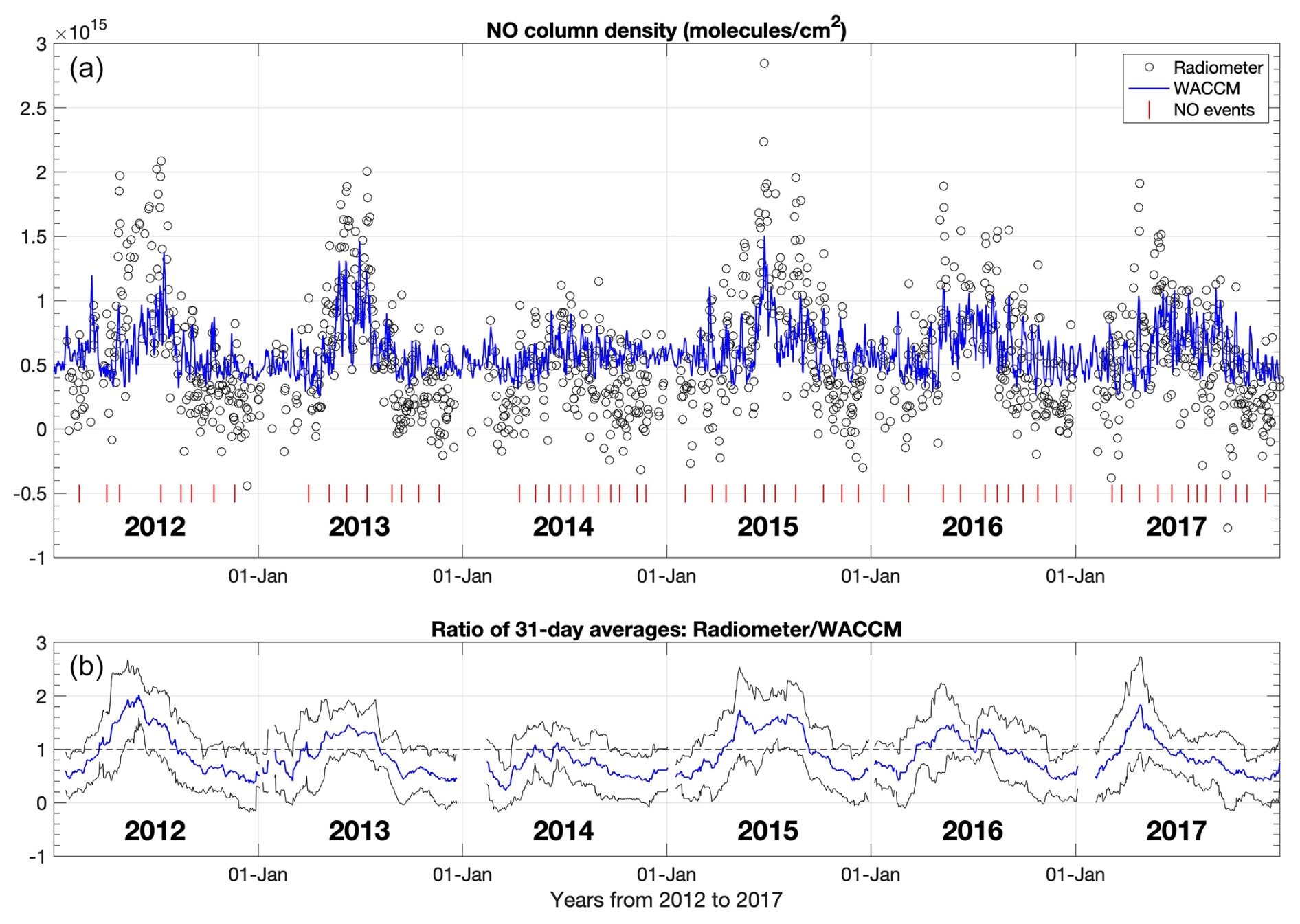
Figure 1 Comparison between Syowa observations and WACCM: (a) daily time series of observed NO column density and simulated column density at 65–140 km. Red marks: the dates of 60 events of observed NO increase, identified in Sect. 3.2 and Table 1. (b) Ratio of observed and simulated 31 d running mean column density. Black lines show the 31 d standard deviation of the observations.

Comparing the simulated column densities to the observations, there is overall agreement in the variability of NO amount between individual winters. However, simulated wintertime values are consistently lower than observed ones and display less pronounced short-term variability. Looking at the ratio of 31 d running averages (bottom panel of Fig. 1), during winter periods the observed column density can be up to a factor of 2 larger, at which times the difference is comparable to, or even exceeds, the standard deviation of the observations. In summer periods, on the other hand, the observations typically show about half of the NO column density compared to simulations.

Figure 2 shows a scatter plot of the observed and simulated daily NO column densities. There is a clear relation between the datasets. The correlation coefficient of r=0.65 is, however, below the 0.7 limit of strong correlation. As already noted above, there is much weaker variability in the simulated column densities. The slope of the linear fit shown in the figure indicates that, overall, only 27 % of the observed range of variability is captured in the simulated data. In addition to showing lower maximum values, the simulated column densities seem to stagnate at the lower end and do not have values smaller than 0.25×10¹⁵ cm⁻². The observed column densities extend to lower values than that, reaching zero and even negative values, with the latter indicating relatively large uncertainties of low summertime NO values. Because these uncertainties could mask some of the natural variability, we tested the robustness of the relation between the datasets by repeating the analysis but including wintertime data only (April–September). We find that the relation remains with only marginal changes (r=0.62).

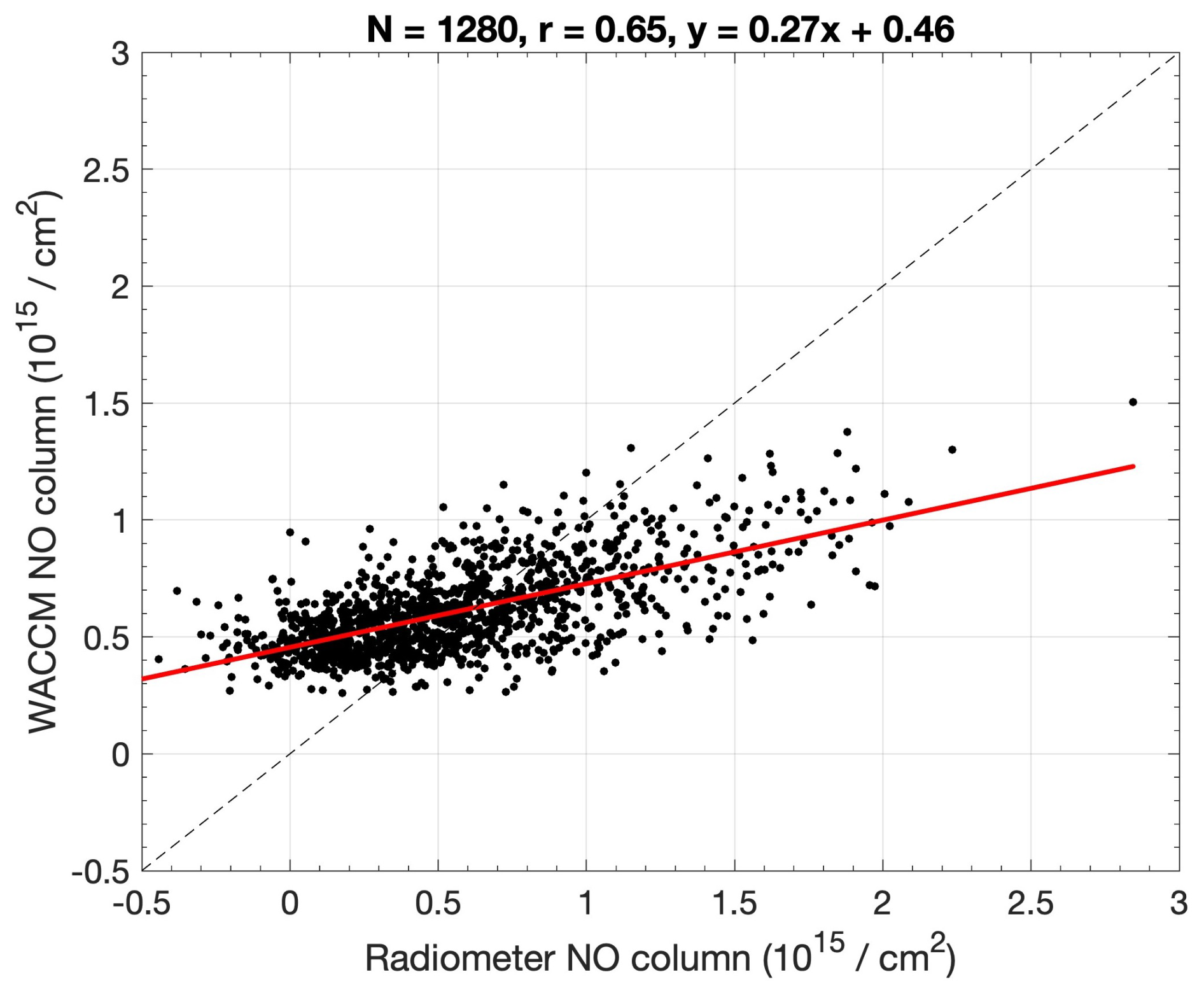
Figure 2 Comparison between Syowa observations and WACCM: relation between the daily NO column densities over the period 2012–2017.

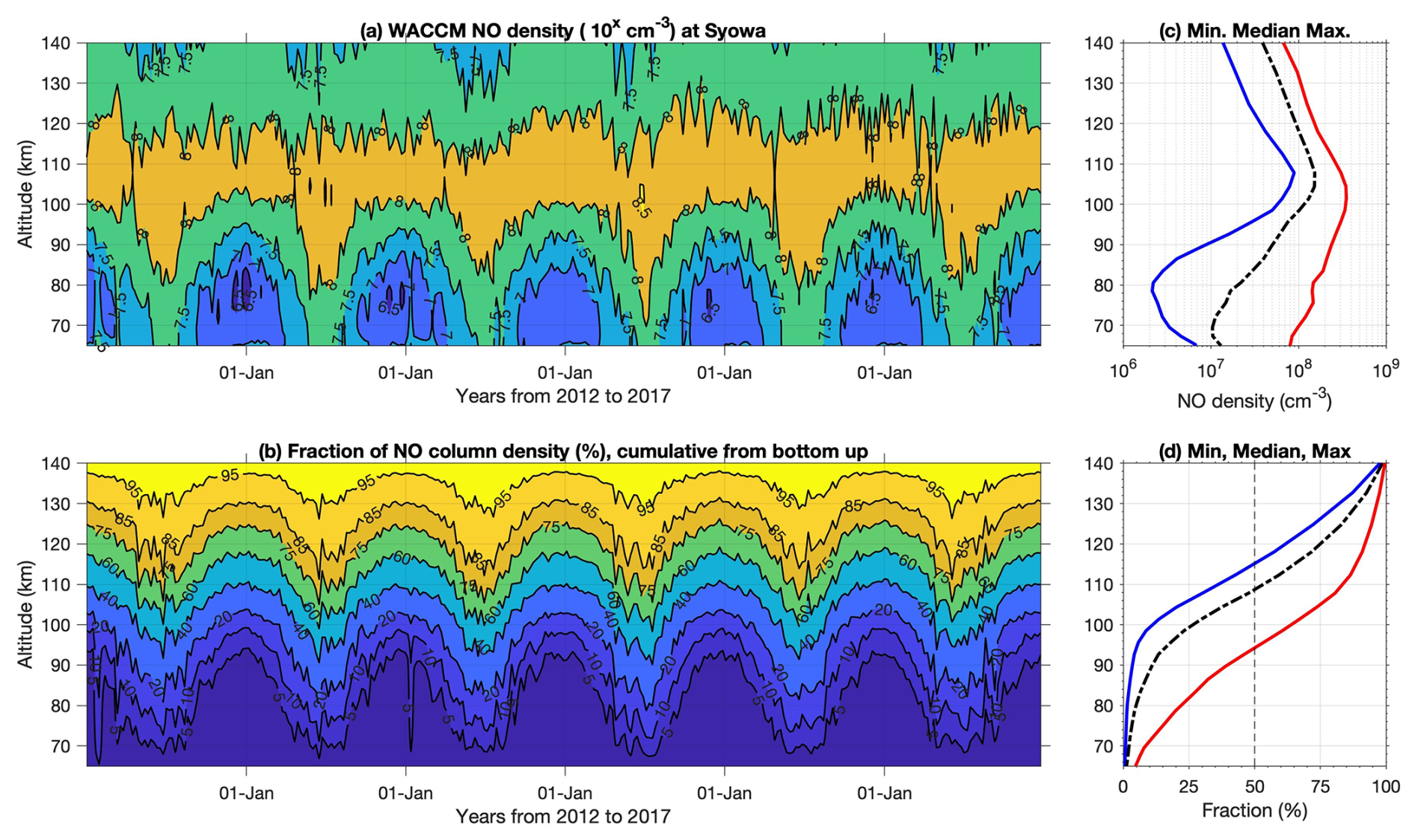
Figure 3 (a) WACCM NO altitude distribution in 2012–2017 at the Syowa station location as a 7 d running average. The contour lines are powers of 10 at 6.5, 7.0, 7.5, 8.0, and 8.5. (b) Fraction of WACCM NO column density from 65–140 km altitude, cumulative from the bottom up, as a 7 d running average. The contour lines are at 5 %, 10 %, 20 %, 40 %, 60 %, 75 %, 85 %, and 95 %. (c, d) Altitude profiles of minimum (blue), median (black), and maximum (red) NO and NO fraction, respectively, over the 2012–2017 period.

To understand the details behind the NO column density and reasons for the variability differences between the observed and simulated data, in the following we make use of the WACCM result and analyze the vertical data profiles from the Syowa location. Figure 3a and c show simulated NO distribution at the 65–140 km altitude range for the years 2012–2017. The NO maximum density is located at about 105 km. Below 100 km, there is a clear variability in NO amount between summer (low NO) and winter (high NO), and the strongest seasonal variability is seen around 80 km altitude. Analyzing the NO column density (Fig. 3b, d), which we calculate by integrating across the altitude range, the 50 %/50 % limit altitude ranges between 94 and 115 km (median = 109 km). At the 50 %/50 % limit, one-half of the total NO column density is from the altitudes above it and another half is from altitudes below it. The limit altitude is lowest in winter periods, which is consistent with the higher NO in the mesosphere contributing more to the total column density. During summer periods, a few short-duration peaks of increased mesospheric contribution can be seen, related to specific precipitation events. For example, the solar proton events of January 2012 and January 2014 can be identified in Fig. 3d, e.g., from a sharp downward peak in the 5 % contour line.

Figure 4 shows the time series of electron forcing, zonal wind speed, and carbon monoxide (CO) mixing ratio from the WACCM simulations, together with the NO column density. The electron impact altitude is dependent on its energy, i.e., higher energy allows for deeper penetration in the atmosphere (e.g., Turunen et al., 2009, Fig. 3). Looking at the altitude distribution of electron ionization applied in WACCM (Fig. 4b), a major part of the ionization is at altitudes above 100 km caused by the Kp-driven auroral electron forcing. This indicates that lower-energy electrons (E∼1 keV rather than ∼10 keV) control a major part of the NO production in the model. This also suggests that the stagnation of simulated NO values at 0.25×10¹⁵ cm⁻² is a result of the auroral electron ionization, which is never less than 10³ ${\mathrm{cm}}^{-\mathrm{3}}{\mathrm{s}}^{-\mathrm{1}}$. Although there is generally a smaller magnitude of variability above 100 km than below, the peak ionization periods above and below 100 km occur very much at the same times and also coincide with increased NO values (Fig. 4a).

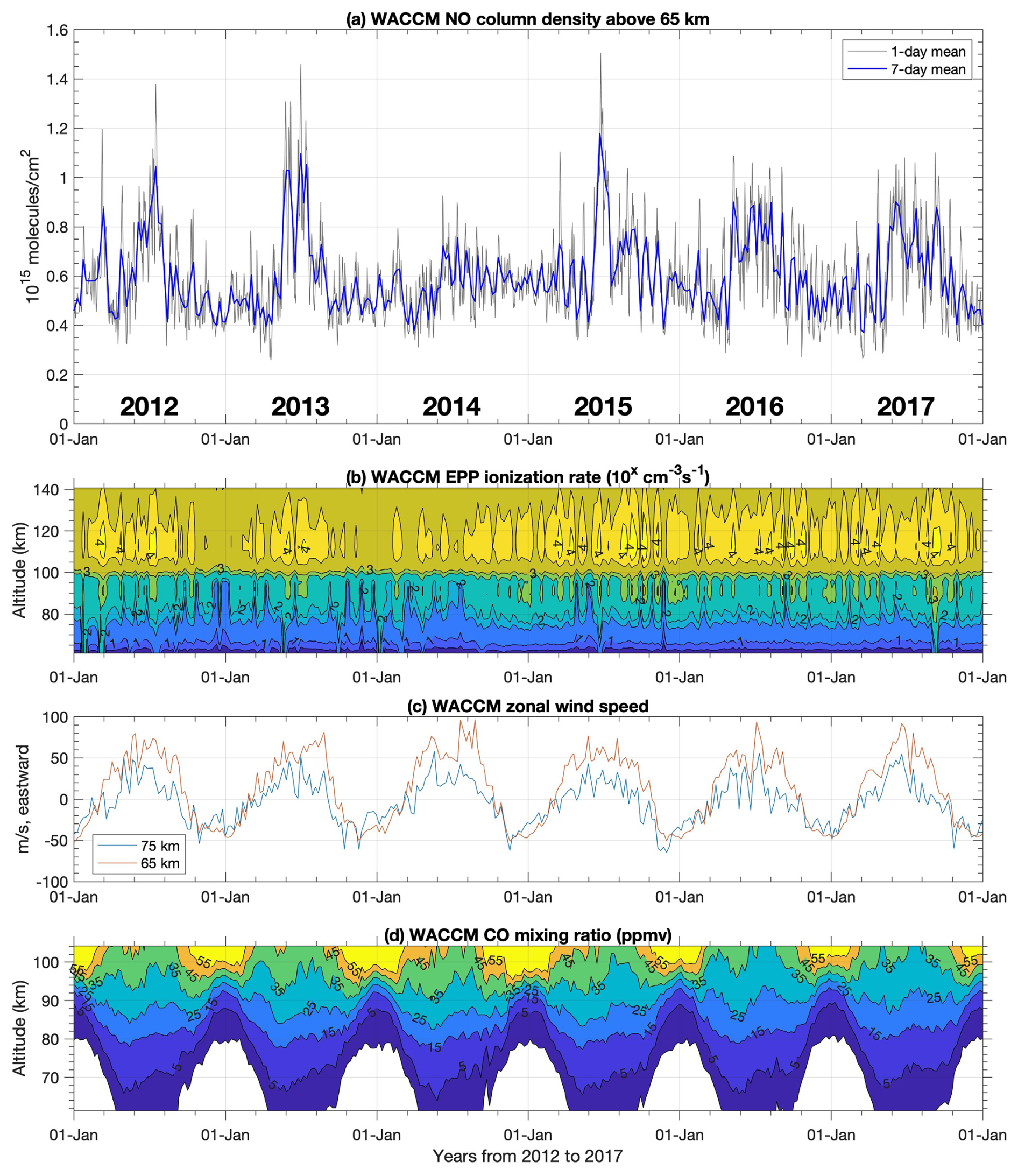
Figure 4 WACCM time series from 2012 to 2017 at the Syowa station location: (a) NO column density and (b) electron ionization rate as a 7 d running average. Contour lines are powers of 10 at 0.5, 1.0, 1.5, 2.0, 2.5, 3.0, 3.5, and 4.0. (c) Zonal wind speed as a 7 d running average. (d) CO mixing ratio as a 7 d running average. Contour lines are at 1, 5, 15, 25, 35, 45, and 55 ppmv. White areas indicate mixing ratios smaller than 1 ppmv.

The auroral electron forcing used in WACCM thus provides stronger ionization and NO production in the lower thermosphere than the medium-energy electron ionization at the mesopause and below. Of the summertime NO column density (Fig. 3b, d), only about 15 % is coming from below 100 km, while in the winter this fraction can be up to about 60 %. This kind of seasonal variability is not seen in the electron ionization rates. The fact that the mesospheric contribution to the NO column density varies so much with the season is a result of a longer chemical lifetime (months), which allows transport and diffusion of NO into the mesosphere from higher altitudes, effectively taking place during winter periods. Figure 4c and d, similar to the observations presented by Isono et al. (2014b, Fig. 5), show that in WACCM high amounts of wintertime NO coincide with eastward winds and high amounts of CO in the mesosphere, indicating the presence of a polar vortex and air descent through the mesopause, respectively. In the summer, winds are westward, mesospheric CO is low, photodissociation reduces the NO chemical lifetime (days), and the effect of NO transport is much smaller. Thus the thermospheric contribution to the NO column density becomes larger.

3.2 Daily NO variability during EEP events

Short-term variability of observed NO column densities, especially strong increases on daily timescales, has previously been attributed to energetic electron precipitation (EEP) ionization events (e.g., Isono et al., 2014a; Newnham et al., 2018). Thus understanding the EEP forcing and its contribution to NO column density is essential at the latitudes under EEP forcing, as at the latitude of the Syowa station. Here we particularly want to assess the EEP forcing and NO short-term variability in WACCM at the Syowa location.

EEP proxy models, e.g., van de Kamp et al. (2016), often use a geomagnetic index as a driver to obtain a statistical representation of EEP forcing in atmosphere and climate simulations. But for individual events, the index that best represents the EEP characteristics such as magnitude and duration likely varies from event to event (Nesse Tyssøy et al., 2019). So, it is interesting to analyze how large daily NO increases seen in the Syowa radiometer observations and WACCM simulations depend on geomagnetic indices.

To find the strongest events of NO production from the observations, for each day we calculate the difference between the 1 and 31 d running averages of the Syowa NO column density data. The largest differences then indicate the strongest daily increases in NO column density. There are a total of 614 daily NO observations that are larger than the corresponding 31 d running mean. However, from these we select only those observations that meet all of the following criteria: (1) the peak NO increase is larger than the corresponding 31 d running standard deviation, (2) the peak day is more than 15 d from any larger peak, and (3) there are more than 10 daily values in the surrounding 31 d period. The first requirement screens out those days on which the NO increase is smaller than overall NO variability and thus less likely to be strongly affected by EEP. The second requirement ensures that events are only counted once. The third requirement screens out periods where robust assessment is potentially restricted by a small amount of data. The list of the 60 identified events, i.e., meeting all criteria, is given in Table 1, and the event peak dates are also marked in Fig. 1. As an example, the event of June 2015 is shown in Fig. 5. It is the largest event identified in the 2012–2017 period with an increase of 1.41×10¹⁵ cm⁻² above the 31 d mean on day 24.

Table 1 List of selected NO increase events from the Syowa column density observations in 2012–2017. The peak NO value is the difference between 1 and 31 d NO column densities. The best correlations with the geomagnetic indices are listed over the 31 d period around the peak day, together with corresponding lags. The dates of the events are marked in Fig. 1.

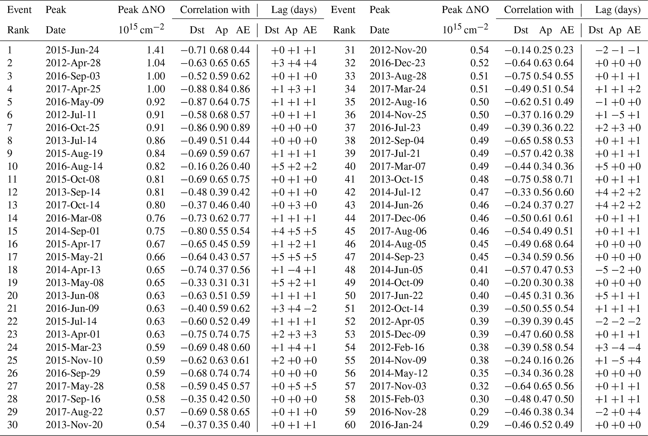
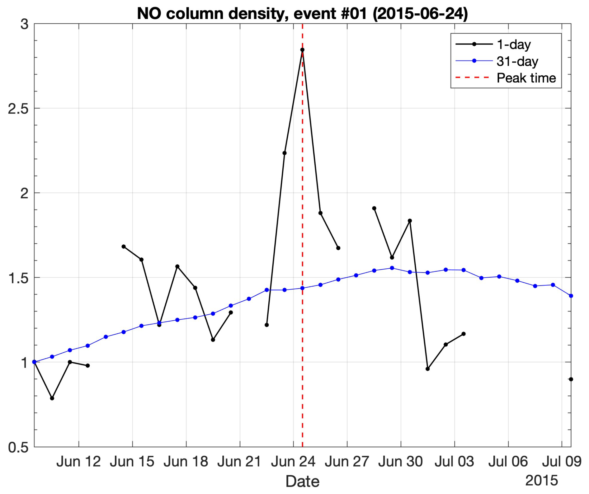
Figure 5 The largest NO increase event from the Syowa column density observations in 2012–2017. Both the 1 and the 31 d average NO is shown for the event period. The event day is marked with a red vertical line.

Not all of the listed NO increases are necessarily EEP-driven because, e.g., polar vortex dynamics contribute to the NO variability. Later, in Sect. 3.4, we discuss the role of polar vortex with some examples. However, here we use geomagnetic indices to relate NO increase events to EEP and geomagnetic disturbances. Geomagnetic indices provide a measure of magnetic activity in the Earth's magnetosphere (e.g., Menvielle et al., 2011). Linked quantitatively to different current systems in the magnetosphere–ionosphere, they are related to different processes, different types of magnetic storms, and particle precipitation with different characteristics in terms of atmospheric forcing (e.g., Turunen et al., 2009). Figure 6 presents two selected events from the 2012–2017 period, showing both the observed and simulated differences in NO column density together with the geomagnetic Ap, Dst, and AE indices. These indices were selected because previous studies have discussed their connection to the precipitating energetic electron fluxes (Isono et al., 2014b; van de Kamp et al., 2016; Nesse Tyssøy et al., 2021a). Note that the simulated NO can be expected to follow the changes in the Ap index because in WACCM daily Ap and Kp are used as the proxy to drive ApEEP and auroral electron ionization, respectively.

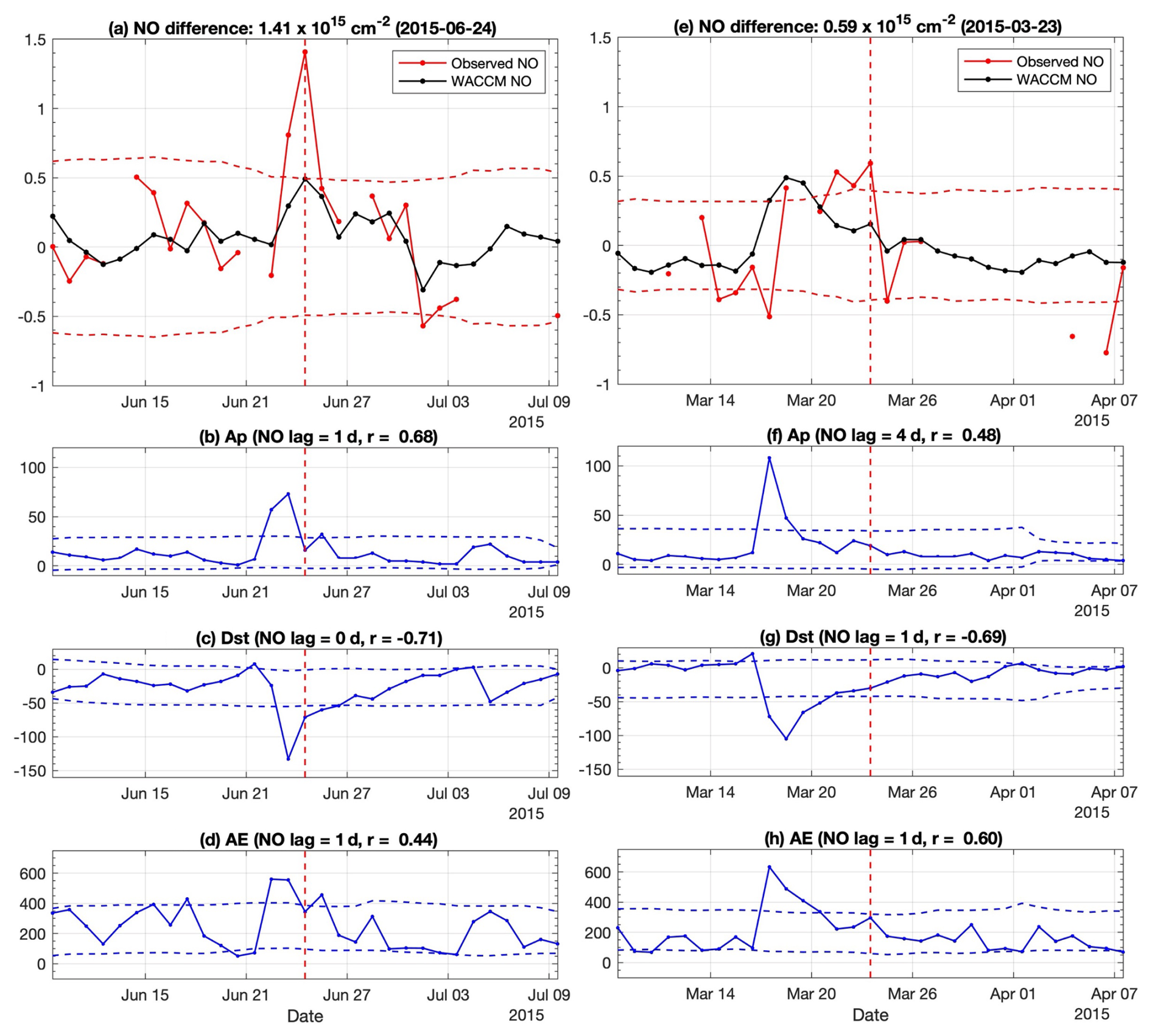
Figure 6 NO increase events #01 (left) and #24 (right): (a, e) observed and simulated NO difference between 1 d and running 31 d averages. Dashed lines indicate the running 31 d standard deviation of observations. Panels (b, c, d) and (f, g, h) show geomagnetic Ap, Dst, and AE indices for the event period. Dashed lines indicate the standard deviation range of the 31 d running mean. The maximum correlation r and the corresponding lag between the index and the observed difference are given in the panel title.

The observed NO shows a response to Ap increase, characterized in many cases by a strong, single peak with elevated amounts around it. This is seen, e.g., in June 2015 (Fig. 6, left panels). There is in many cases a 1 d lag between the Ap peak and the peak NO increase, which can be explained by accumulation of NO during an EEP forcing. The strongest correlations are therefore typically found between NO and the previous day's Ap. Compared to observed NO increases, in general WACCM data show similar peaks of NO but underestimate the magnitude of increase by a factor of 2–3. However, the overall day-to-day variability is typically well represented in WACCM. In the case of June 2015, correlation with Dst is slightly stronger than with Ap and there is no lag (note that the Dst index during magnetic storms has a negative sign).

As seen from Table 1, the list of the largest events includes mostly autumn to spring months at Syowa (April–November). Summer months and winter months are equally likely to have EEP-driven NO events but the summer events would, in theory, be easier to detect due to the lower 31 d background. However, observations of lower NO amounts have a poorer signal-to-noise ratio. Also, the shorter chemical lifetime due to enhanced photodissociation in summer compensates for NO increases faster. This means that some of the largest events could go undetected in the NO observations. If we consider the 30 largest events only, the seasonal distribution peaks in April and September, which is consistent with the known seasonal variability in magnetic activity and EEP forcing (e.g., Tanskanen et al., 2017).

An example of an autumn case is the St. Patrick's Day event in March 2015 (Fig. 6, right panels). Although this was a major event reported in many studies, e.g., Clilverd et al. (2020), it ranks only at #24 in our Table 1 with an increase in NO by 0.59×10¹⁵ cm⁻². Interestingly, in terms of simulated increase this event is quite similar in magnitude to the June 2015 event, which suggests that this was indeed a major event also from NO point of view.

A feature seen during the March 2015 St. Patrick's Day event is that the NO increase clearly has a shorter duration in the simulated data when compared to the observations. The simulated NO and observed NO have a similar buildup until day 18. However, simulated NO has already decreased before the observed maximum on day 23. The simulated NO follows Ap, which has a sharp peak on day 17. In this case, the maximum correlation between Ap and observed NO is 0.48 with a 4 d lag. In contrast, the Dst index has a peak on day 18 and recovers slower than Ap over the following 6–7 d. Correlation between Dst and NO is largest at −0.69 with 1 d lag. Similarly, the correlation between AE and NO is stronger than between Ap and NO. Therefore, during this event the temporal behavior of NO follows the Dst and AE indices more closely than it follows the Ap.

To understand the overall relation between EEP forcing as represented by different geomagnetic indices and NO increases at Syowa, we calculate correlations and lags between NO and three indices: Ap, Dst, and AE. For the events listed in Table 1, we present the distribution of 31 d correlation coefficients and corresponding lags between the indices and NO in Fig. 7. For reference, we also present here the distribution of correlations and lags between simulated NO and the Ap index. This provides a measure of an “optimal” case because in WACCM EEP forcing is driven by the Ap and Kp indices.

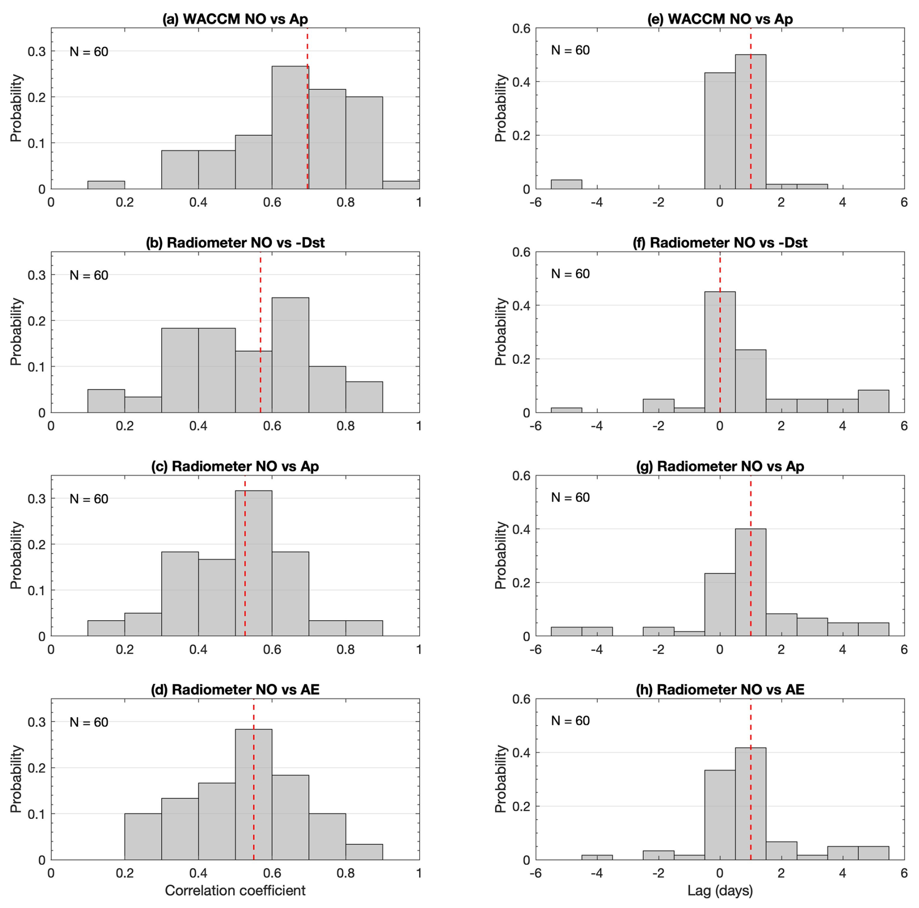
Figure 7 Histograms for the NO increase events (N=60, see Table 1). Correlation (left) between geomagnetic indices and daily NO column density, with the (right) corresponding lag (days). In all panels, the vertical red line indicates the median of 60 events.

Comparing the distribution of correlation coefficients r, NO column density variability is clearly related to all three indices. The median is lowest at 0.53 with Ap and at maximum at 0.57 with −Dst. There are clear differences in the r distribution, however. Correlation with −Dst is strong, i.e., larger than 0.7 in 17 % of cases, while this probability is 13 % with AE and just 7 % with Ap. On the other hand, the correlation with Ap is more concentrated in the 0.5–0.6 range and thus, in a sense, more consistent throughout the events. As expected, the median correlation between Ap and WACCM NO is strong at 0.70 and exceeds those between NO observations and the indices. 43 % of the events have a correlation stronger than 0.7 between Ap and WACCM NO.

For the lag corresponding to the best correlation, the results are very similar for all indices. The lag is either 0 or 1 d for the majority (63 %–75 %) of the events, depending on the geomagnetic index. Median lag is 1 d with Ap and AE and 0 d for Dst. A 1 d lag is consistent with the chemical lifetime of NO and results from previous studies (e.g., Solomon et al., 1999). When a daily average is used, Dst covers both the initial and main phase of the geomagnetic storm, which likely explains why the most probable lag is 0 instead of 1 d. A lag of 2 or more days is seen in 18 %–25 % of the events, again depending on the index used. The median lag between Ap and WACCM NO is also 1 d, consistent with the lag seen in the observations. However, in WACCM data only 3 % of the cases have a lag of 2 or more days.

3.3 Sensitivity to medium-energy electron forcing

As discussed in Sects. 2.2 and 3.1, a considerable contribution to the simulated NO column density is from thermospheric production by EEP ionization. From a previous study in the Southern Hemisphere, however, there is also evidence of an overestimation of polar thermospheric NO in WACCM simulations when compared to satellite-based observations, while, on the other hand, mesospheric NO seems to be underestimated (Newnham et al., 2018). Therefore, in order to increase NO column density during EEP events, we proceed here to assess the contribution of medium-energy electron (MEE) forcing. There are also other reasons to focus on MEE forcing. One is the remaining discrepancies between datasets (Sinnhuber et al., 2021), which indicates significant uncertainties in MEE forcing when applied in atmospheric simulations. Another is that a lot more variability can be expected from higher-energy EEP compared to EEP at auroral energies, so improving MEE forcing would also likely help to improve the NO variability.

To assess the sensitivity to the impact from MEE in WACCM simulations, we make use of electron fluxes measured by instruments on board the Arase (ERG) satellite (see Sect. 2.3 for details). Arase measurements are available from March 2017 onwards. Thus we are only able to assess the impact from Arase-measured electron fluxes from May to December 2017. From Fig. 1 and Table 1, there are several events of NO increase identified in this period. Selecting from these, based on flux data availability and preferring wintertime occurrence, we proceed to use Arase-based fluxes for six events (#13, #27, #28, #29, #39, #50). These events begin at the end of May and continue monthly until November. For each of the event periods (6 d each), the WACCM ApEEP MEE forcing was replaced by those calculated from Arase electron flux data. The WACCM simulations were then repeated from April to December 2017, and the impact on NO column densities at the Syowa station was assessed. We can perhaps expect an NO increase from the Arase-based electron fluxes, also because Arase measurements include both precipitating and trapped electron fluxes in the radiation belt, while only the precipitating electrons will produce an atmospheric impact.

As an example, Fig. 8 shows Arase electron flux measurements from 22 July 2017 and resulting ionization rates at magnetic L shell 6.2 near the Syowa station. In general, the Arase-based ionization tends to exceed the ApEEP MEE ionization in the middle-mesospheric altitudes, while around the mesopause the ApEEP-driven ionization and in the lower thermosphere the Kp-driven auroral ionization used in the original WACCM simulation are stronger. Due to the high-energy limit of 500 keV of the Arase measurements used here, ApEEP ionization rates are larger in the lowermost mesosphere. Thus, when applied in WACCM simulations, the Arase-based ionization does not necessarily increase mesospheric NO production or the mesospheric contribution to the NO column density. Although this is a typical example, we note that overall there is larger temporal variability in the Arase-based ionization rates compared to those from the statistical ApEEP model. Here it should be noted, based on Fig. 1, that the year 2017 was not a high-NO year and the overall NO variability was moderate compared to some previous years (e.g., 2015). We are, however, restricted to 2017 due to Arase data availability.

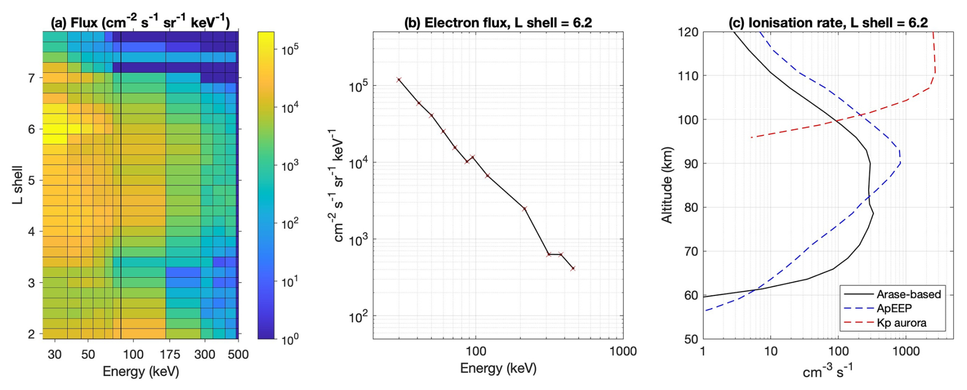
Figure 8 An example of Arase electron flux measurements and corresponding atmospheric ionization. (a) Average electron fluxes on 22 July 2017 at 06:00–18:00 UT. (b) Arase electron fluxes at L shell 6.2. (c) Arase-based ionization rates at L shell 6.2, together with ApEEP v1 and Kp aurora ionization from WACCM.

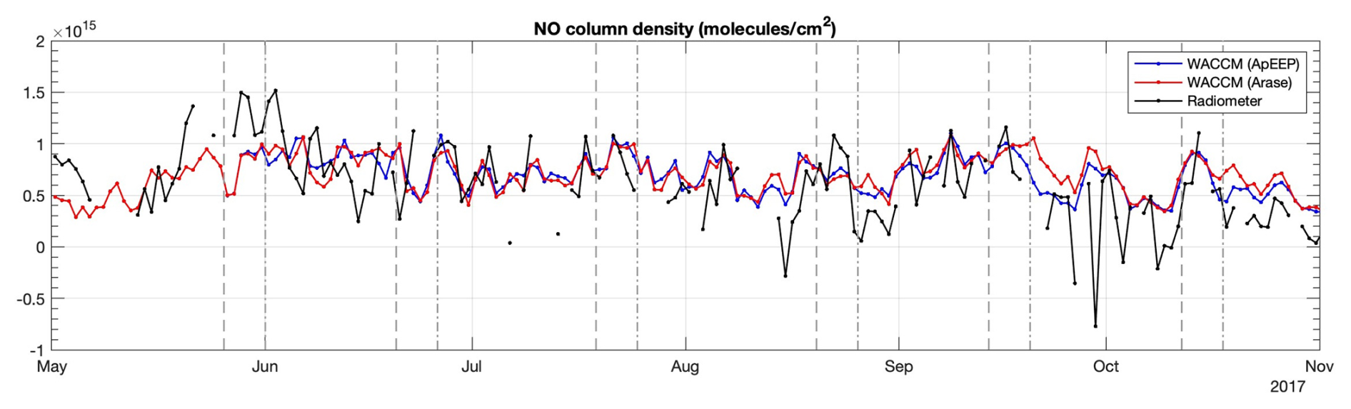
Figure 9 Daily time series of NO column density in 2017: Syowa radiometer observations and two WACCM simulations with different electron forcing (ApEEP v1; Arase-based trapped fluxes). The radiometer and WACCM (ApEEP) data are the same as those shown in Fig. 1. Dashed and dash–dot lines mark the start and end times of the Arase-based electron forcing.

In Fig. 9, we compare the Arase-driven NO column density to the radiometer observations and the original WACCM simulation. During all the event periods from May to August, there is clearly a smaller difference between the two simulations than between the simulations and the radiometer observations. The largest differences between the two simulations are seen during/after the September and October events, but then the Arase-driven simulation is in less agreement with the observations than the original simulation. Following the end-of-May event, the simulated NO now reaches 1.0×10¹⁵ cm⁻², while NO is below that in the original simulation. However, this increase is seen on a few days only, is relatively small, and does not significantly improve the agreement with the radiometer measurements, which reach up to 1.5×10¹⁵ cm⁻². Thus, despite differences in the altitude distribution of electron ionization, the variability of NO column density during the end-of-May event is also underestimated in the Arase-based simulation. On the other hand, the overall agreement in NO between the original simulation driven by a proxy EEP model and the Arase-driven simulation gives confidence in both datasets and suggests that Arase electron flux observations can be useful in atmospheric simulations.

3.4 Role of the polar vortex

As mentioned earlier, atmospheric dynamics also contribute to NO variability, especially in wintertime when NO chemical lifetime is months and it can accumulate inside the polar vortex. When considering the NO column density above 65 km, as measured by the Syowa radiometer, it must be noted that the polar vortex only exists in the mesosphere but not in the thermosphere. Thus only a fraction of the NO column density is potentially affected by the polar vortex. However, this is the fraction which is also directly impacted by > 30 keV, medium-energy electrons.

The Syowa station is located in the polar region at 69° S (geographic). Overall, based on 13 years of reanalysis data (Harvey et al., 2018), from March to August the station is most of the time located inside the mesospheric polar vortex where larger amounts of accumulated NO are expected. Nevertheless, day-to-day variability in vortex dynamics could lead to NO variability at Syowa and mask the variability driven by EEP. As an example, Fig. 10 presents the vortex edges for the event of June 2015 (the largest event identified in Sect. 3.2). We calculate them from daily average WACCM CO maps at 0.015 hPa (≈ 74 km in June) using the chemical definition method for the mesospheric polar vortex as presented by Harvey et al. (2015). This method does not rely on the horizontal wind fields, which can be complicated in the mesosphere and lead to spurious day-to-day changes in vortex area. Although the following discussion is based on simulated data, we note that in the mesosphere WACCM can reproduce observed winter vortex size and frequency of occurrence reasonably well (Harvey et al., 2019).

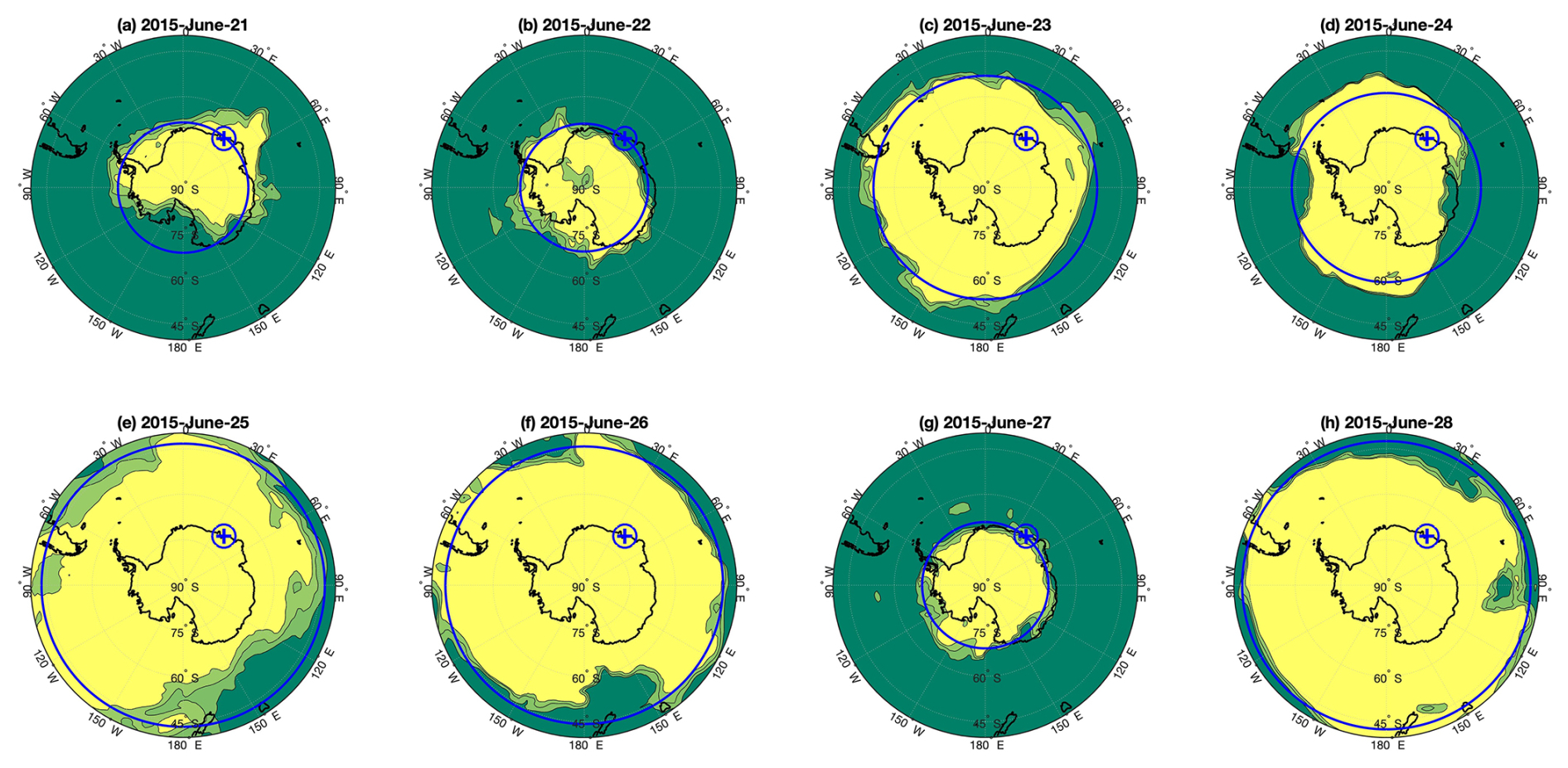
Figure 10 Polar vortex edges calculated from WACCM CO data for selected days around event #1 (peak NO day: 24th). Yellow, light green, and dark green areas are inside, on the edge, and outside of the vortex, respectively. The blue cross marks the Syowa location, and the large blue circle is at the equivalent latitude of the polar vortex area. Latitudes larger than 40° S are shown.

Figure 10 shows how in the simulations the polar vortex evolves from day to day during the June 2015 event. On 6 out of the 8 d presented, including the peak NO day (day 24), Syowa is clearly inside the vortex. On days 22 and 27, Syowa is close to the vortex edge. However, these 2 days do not show particularly high or low NO column density values in simulations or observations (see Fig. 6). Rather, the NO column density values on these 2 days are closer to the 31 d mean than on most other days. Nevertheless, it seems possible that in this case mesospheric vortex dynamics might play an important role for NO column density variability because the high-NO days are inside the vortex. On the other hand, over the 31 d period around the NO peak Syowa is outside the vortex on 7 d only, which indicates that the NO column density reference that we use when identifying NO increase events is calculated mostly from values measured inside the vortex.

Using the WACCM CO, we assess the Syowa station location in relation to vortex edges for all event periods on a daily basis to determine if the station was inside or outside of the vortex. Overall for all 60 events, Syowa is inside (outside) of the vortex on 48 % (18 %) of the peak NO days. In the other 34 % of cases, there is no vortex edge identified on the peak day; i.e., either CO does not have a maximum in the polar regions or CO gradients are not strong enough. As can be expected, the no-vortex cases take place in and around summer periods and there are in fact no such cases from April to August. Figure 11 presents the histograms for those events (N = 47) that have Syowa inside the polar vortex at least on 1 d during the surrounding 31 d period. These events are relatively evenly distributed from March to October, i.e., in autumn, winter, and spring periods. On the peak NO day, 62 % (23 %) of the events Syowa are inside (outside) of the vortex. 15 % of the events have no vortex identified on the peak day. The median number of vortex occurrence days at Syowa over the corresponding 31 d periods is 23. Thus, there is a considerable proportion of events identified even if Syowa is not always inside the vortex. It seems that the mesospheric vortex impact on the lower half of the NO column plays a lesser role than the EEP forcing, which affects the full column density above 65 km.

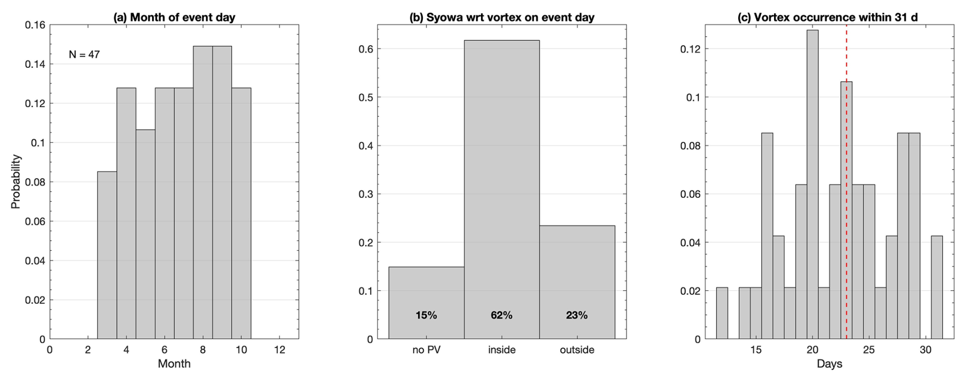
Figure 11 Histograms for NO increase events (N=47; the vortex is present on at least 1 d within the 31 d period surrounding the event). (a) Monthly distribution of NO peak day, (b) Syowa location with respect to the polar vortex on the peak day, and (c) number of vortex occurrence days within the surrounding 31 d period. The vertical red line indicates the median of 47 events.

On longer timescales, year-to-year variability in the polar vortex occurrence rate and extent could affect the amount of overall wintertime NO observed at the Syowa station. As seen in Fig. 1, during the winter of 2014 the radiometer measured clearly less NO than during 2013 or 2015, a feature also seen in the WACCM data. Based on the vortex data calculated from the WACCM daily CO in the mesosphere, there was little difference between the winters in terms of the polar vortex characteristics. The number of vortex occurrence days is 164, 158, and 178 in the winters of 2013, 2014, and 2015, respectively. Of those days, the equivalent latitude of the vortex edge is Equatorward of 69° S on 110, 105, and 126 d, respectively. The median equivalent latitude of the vortex edge is 57, 61, 58° S, respectively. These relatively small differences in vortex occurrence rate and extent indicate a minor impact on the NO column density. Thus the lower EEP forcing remains a major reason for lower NO column density in 2014, which agrees with the NO results from the Halley station reported by Newnham et al. (2018).

4 Discussion

One of the open questions in EEP atmospheric impact research has been to understand the differences in both the amount and vertical distribution of NO in the mesosphere–lower thermosphere (MLT) region seen between different sets of observations and models (Randall et al., 2015; Hendrickx et al., 2018; Sinnhuber et al., 2021). Since the radiometer NO column density observations do not include information on the NO altitude distribution, they are best used to understand the overall NO content, which is a measure of the full EEP forcing in the MLT. Comparing these observations with WACCM results, and analysis of the NO altitude distribution in the model, allows us to investigate the reasons behind any differences between model data and observations. While the radiometer data are limited in altitude information, they provide a continuous local view which is not available from satellite-based observations.

Here we have found that the key discrepancy is in the amount of NO in the MLT; e.g., the highest simulated wintertime amounts do not reach those measured. On the other hand, the year-to-year and day-to-day NO variability is qualitatively well-presented. This suggests that the electron energy input in the atmosphere is underestimated in our simulations, which apply the current recommendation of electron forcing. After the initial work on solar particle forcing (Matthes et al., 2017), a revision is currently being finalized for the Coupled Model Intercomparison Project Phase 7. Considering the increased electron forcing in several new datasets when compared to the ApEEP model (Nesse Tyssøy et al., 2021b), the new forcing recommendation is expected to increase the production and amount of NO in simulations. Based on our results here, an increase in electron forcing is well justified.

As reported by Newnham et al. (2018), the BAS radiometer measured NO Antarctic column density at the Halley station (75.6° S, 26.3° W). During 2013–2014, the measurements showed strikingly different winters of high and low NO column density, similar to what we show here for Syowa in Fig. 1. Comparing the Syowa observations to the NO amounts shown by Newnham et al. (2018) in their Fig. 4, there is overall agreement between the two datasets. The highest NO column densities are consistently above (below) 1.0×10¹⁵ cm⁻² in 2013 (2014). The agreement indicates that the NO column density at a location, such as Syowa, is a reasonable representation of the polar cap situation, although we have to note that there are differences in magnetic latitude and geographic location of the two radiometers.

We have shown that the NO column density at Syowa correlates similarly with the Ap, AE, and Dst indices. Although the indices correspond to different processes related to different EEP characteristics, finding such agreement is perhaps not surprising. Especially in winter, accumulation and transport of NO will have an impact on its distribution and weaken the direct links to the detailed temporal and spatial extent of EEP. Also, van de Kamp et al. (2016) have shown that statistical models based on same electron flux data but driven by Ap and Dst indices perform almost equally well. Thus, it seems that the choice of proxy for EEP seems to be of less importance than having good-quality electron flux data to accurately represent the magnitude of forcing.

We have found that the Arase electron flux measurements made in the radiation belt indicate different characteristics of mesospheric electron forcing compared to the ApEEP MEE model. Particularly, in many cases Arase data indicate more (less) atmospheric ionization at middle- (upper-)mesospheric altitudes. When the Arase-based ionization is applied during specific events, it does not improve the day-to-day variation of simulated NO column density when compared to the radiometer observations. Instead, the two simulations are rather close to each other, which gives some confidence to both datasets. While this preliminary study was done in 2017, which had relatively low geomagnetic activity, we expect that the variability of NO column density will be more sensitive to the changes introduced in mesospheric electron forcing during more active years. It should be noted that characterization of electron precipitation from the fluxes measured in the radiation belts, as Arase does, would benefit from additional measurements that allow the trapped fluxes to be removed. This kind of approach has been demonstrated in a recent study by Duderstadt et al. (2021), who used a combination of observations from the Van Allen Probes and the Firebird II small satellite to estimate electron forcing on the atmosphere. A similar approach could be potentially developed using the Arase electron flux measurements. In addition, there are some issues related to the MLT and L-shell coverage of the observations (see Sect. 2.3) that could be addressed to improve the usability of Arase data in atmospheric simulations. Detailed consideration of these is, however, outside the scope of this study.

It is evident from our results that the maximum and minimum values of NO day-to-day variability are not well captured in WACCM. Driven by the Ap and Kp indices, the proxy EEP models used in WACCM are statistical average models which by their nature provide a smoothed impact of the measured electron forcing. Instead of using statistical proxy models, electron flux observations can be used directly for those time periods when data are available. However, this is not an option for climate simulations, which are typically extended beyond the temporal limits of observations (Matthes et al., 2017). As a next step, a stochastic approach, sampling on measured distributions of electron forcing, could be a useful method to capture the extremes of variability better and to improve the representation of atmospheric impacts in models.

5 Conclusions

We have compared the mesosphere-to-thermosphere NO column densities from the Syowa radiometer and WACCM.

1. Qualitative agreement on year-to-year and day-to-day NO variability exists between the radiometer and WACCM. However, compared to the observations, the simulated 31 d averages are up to a factor of 2 smaller (larger) in the winter (summer) periods. The magnitude range of daily NO column densities is much larger in the observations, and the simulation captures just 27 % of the observed variability.

2. Observed day-to-day variability is driven by EEP forcing. During time periods of identified EEP events (N = 60), the NO column density correlates with the Ap, Dst, and AE geomagnetic indices (with median $r=\mathrm{0.53},-\mathrm{0.57},\mathrm{0.55}$, respectively), with a 0–1 d lag. WACCM reproduces the observed day-to-day variability in most cases but with a diminished magnitude.

3. The relatively small variability in mesospheric polar vortex occurrence rate and extent does not indicate a large impact on the winter-to-winter or day-to-day NO column density variability at the Syowa location.

4. Results from a simulation using Arase-based EEP forcing, based on precipitating and trapped electron flux measurements, demonstrate the potential of such measurements in atmospheric research. More research on the variability of the NO column density is needed, including on the impact from high-energy electrons (> 30 keV) directly affecting the mesosphere.