Observations of traveling ionospheric disturbances driven by gravity waves from sources in the upper and lower atmosphere

The observed traveling ionospheric disturbances (TIDs) are attributed to atmospheric gravity waves generated by auroral sources in the lower thermosphere or gravity waves generated in the troposphere by midlatitude weather systems. TIDs are observed by the Poker Flat Incoherent Scatter Radar (PFISR), the Super Dual Auroral Radar Network (SuperDARN), multipoint and multifrequency continuous Doppler sounders, and Global Navigation Satellite System (GNSS) receivers using the total electron content (TEC) mapping technique. At high latitudes, the solar wind–magnetosphere–ionosphere–thermosphere coupling modulates the dayside ionospheric convection and currents, the source of the equatorward-propagating TIDs. The horizontal equivalent ionospheric currents are estimated from the ground-based magnetometer data using an inversion technique. At midlatitudes, the eastward- to southeastward-propagating medium-scale TIDs that were observed by the high-frequency (HF) Doppler sounding system, as well as in the detrended TEC, are attributed to gravity waves that are generated by geostrophic adjustment processes and shear instability in the intensifying low-pressure systems and are identified in the stratosphere using the ERA5 meteorological reanalysis.

1 Introduction

The theory governing the propagation and effects of atmospheric gravity waves (AGWs) in the ionosphere was developed by Hines (1960), and their ionospheric sources have been recognized (Chimonas, 1970; Chimonas and Hines, 1970; Testud, 1970; Richmond, 1978). The relationship between AGWs and traveling ionospheric disturbances (TIDs) has been well established (Hocke and Schlegel, 1996). Global propagation of medium- to large-scale GWs/TIDs has been linked to auroral sources (Hunsucker, 1982; Hajkowicz, 1991; Lewis et al., 1996; Balthazor and Moffett, 1997). The Worldwide Atmospheric Gravity-wave Studies (WAGS) program (Crowley and Williams, 1988; Williams et al., 1993) showed that large-scale TIDs originate in auroral latitudes.

TIDs driven by AGWs that originate in the lower atmosphere come from a variety of sources, including tropospheric weather systems (Bertin et al., 1975, 1978; Waldock and Jones, 1987; Nishioka et al., 2013; Azeem et al., 2015). Other known causes of AGWs/TIDs are solar flares (Zhang et al., 2019), total solar eclipses (Zhang et al., 2017; Mrak et al., 2018), volcanic eruptions, earthquakes, and tsunamis (Yu et al., 2017; Nishitani et al., 2019; Themens et al., 2022).

Most of the early observations of TIDs were obtained by high-frequency (HF) Doppler sounders, HF radars, and incoherent scatter radars (Hunsucker, 1982). More recently, GNSS-derived (GNSS: Global Navigation Satellite System) total electron content (TEC) measurements have become a commonly used technique to observe medium- to large-scale TIDs (e.g., Afraimovich et al., 2000; Cherniak and Zakharenkova, 2018; Cheng et al., 2021; Nykiel et al., 2024). Large-scale TIDs (LSTIDs) have wavelengths greater than 1000 km and propagate at speeds of 400–1000 m s⁻¹, while medium-scale TIDs (MSTIDs) have wavelengths of several hundred kilometers and tend to propagate at speeds of 250–1000 m s⁻¹ (Hunsucker, 1982).

Van de Kamp et al. (2014) described two techniques to detect TIDs, one using the EISCAT incoherent scatter radar near Tromsø and the other using the detrended GPS TEC data. They determined parameters characterizing TIDs and studied an event on 20 January 2010. While these authors did not investigate the origin of the TIDs they suggested that the AGWs were most likely generated at low atmospheric layers. Using the EISCAT Svalbard radars on 13 February 2001, Cai et al. (2011) observed moderately large-scale TIDs propagating over the dayside polar cap that were generated by the nightside auroral heating. It is noted that both these TID events occurred on days following arrivals of corotating interaction regions (CIRs) at the leading edge of solar wind high-speed streams that triggered moderate geomagnetic storms.

Frissell et al. (2016) concluded that polar atmospheric processes, namely the polar vortex, rather than space weather activity are primarily responsible for controlling the occurrence of high-latitude and midlatitude winter daytime medium-scale TIDs (MSTIDs). This paper has been frequently cited to justify suggestions of the polar vortex as a source of the observed MSTIDs, particularly when geomagnetic activity is low. Recent papers (Becker et al., 2022b; Bossert et al., 2022; Vadas et al., 2023) have discussed methods for assessing vortex-generated GWs from model output. Vadas et al. (2023) discussed observations of polar-vortex-generated GWs and subsequent secondary GW generation in the polar region. Becker et al. (2022a) performed simulations focusing on multistep vertical coupling by primary, secondary, and higher-order gravity waves of wintertime thermospheric gravity waves and compared them with observed perturbations of total electron content. They demonstrated that gravity waves generated from lower altitudes can propagate equatorward. Bossert et al. (2022) discussed a strong TID/TAD event observed during a sudden stratospheric warming (SSW) on 18–19 January 2013 and suggested that the large-scale TIDs/TADs were related to geomagnetic activity despite a low Kp index. Thus, it is important to continue discussing possible sources of GWs in the lower and upper atmosphere.

The solar wind coupling to the dayside magnetosphere (Dungey, 1961, 1995) generates variable electric fields that map to the ionosphere driving the E×B ionospheric convection observed by Super Dual Auroral Radar Network (SuperDARN) HF radars and ionospheric currents observed by networks of ground-based magnetometers. The mechanisms for energy transfer to the thermosphere can be Joule heating, precipitation, or ion drag by Lorentz force (Richmond, 1979; Nishimura et al., 2020; Deng et al., 2019). Nykiel et al. (2024) found that Joule heating is a primary energy source for the nighttime LSTIDs triggered in the auroral region, while the daytime LSTIDs can also be driven by precipitating particles in the polar cusp. On the dayside, pulsed ionospheric flows (PIFs), which are known to be associated with poleward-moving auroral forms (precipitation), have been observed to generate AGWs, which in turn modulate ionospheric densities, resulting in MSTIDs propagating equatorward as observed by SuperDARN radars (Samson et al., 1989, 1990; Prikryl et al., 2005, 2022).

In this study, even in the case when geomagnetic activity is very low, PIFs are found to be the source of AGWs/TIDs observed by PFISR and SuperDARN (Sect. 3.1). In other cases, the AGWs/TIDs that were generated by solar wind Alfvén waves coupling to the dayside magnetosphere are investigated in Sect. 3.2. The equatorward-propagating TIDs were observed in the detrended vertical TEC (vTEC) and the radar ground scatter power focused and defocused by TIDs moving equatorward.

The tropospheric convection is often a source of gravity waves that propagate into the upper atmosphere, driving TIDs (e.g., Azeem, 2021, and references therein). In this study, gravity waves generated in the troposphere by geostrophic adjustment processes and shear instability (Uccellini and Koch, 1987) are considered to drive TIDs propagating eastward to southeastward that were observed in the detrended vTEC maps and by the HF Doppler sounding system (Sect. 4). To our knowledge, this physical mechanism has not been considered as a source of TIDs. The ERA5 meteorological reanalysis is used to show the gravity waves propagating into the stratosphere.

The aim of this study is to attribute the observed TIDs to sources in the upper (Sect. 3) and the lower (Sect. 4) atmosphere. These observations show that AGWs provide both downward and upward vertical coupling of the ionosphere and neutral atmosphere.

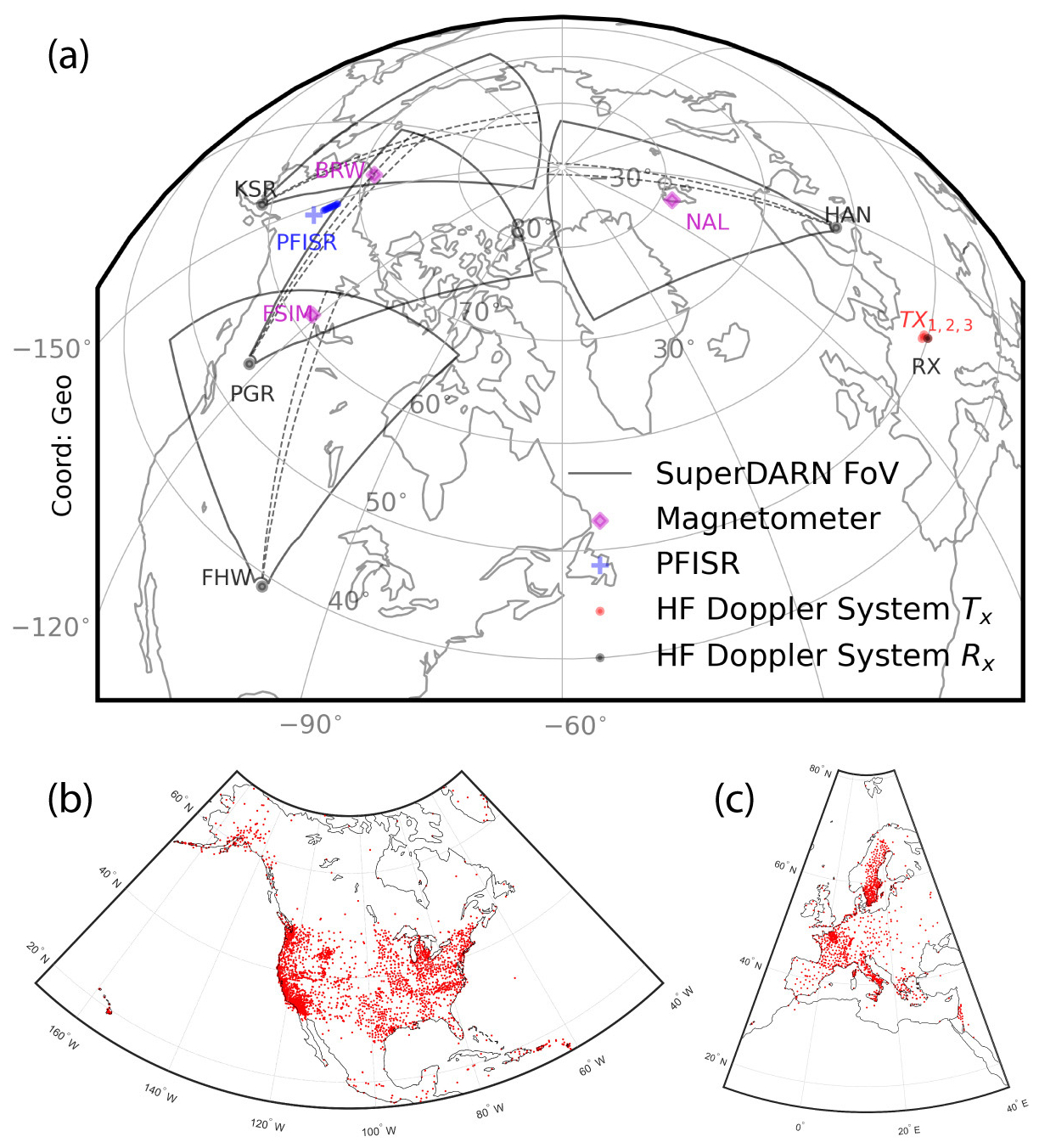
Figure 1 (a) The fields of view of SuperDARN radars in King Salmon (KSR), Prince George (PGR), Fort Hayes West (FHW), and Hankasalmi (HAN) are shown in black. The Poker Flat Incoherent Scatter Radar (PFISR) beam 2 range gate footprints are shown in blue. Also, the ground magnetometers in Barrow (BRW, now Utqiaġvik), Fort Simpson (FSIM), and Ny-Ålesund (NAL) and the locations of transmitters (T_X) and a receiver (R_X) of the HF Doppler sounding system operating in the Czech Republic are shown. (b, c) Examples of the GNSS station distribution in the two local domains of interest, when there were 5708 stations available globally.

2 Data sources and methods

Figure 1 shows a map of instruments used in this study as described below.

2.1 Advanced Modular Incoherent Scatter Radar

Data from the Advanced Modular Incoherent Scatter Radar (AMISR) located in Poker Flat, AK (i.e., the Poker Flat Incoherent Scatter Radar – PFISR), were used in this study. AMISR uses phased-array beam-forming techniques on a pulse-to-pulse timescale to effectively sample various look directions simultaneously (Heinselman and Nicolls, 2008). These radars have been used to investigate gravity wave propagation (Nicolls and Heinselman, 2007; Vadas and Nicolls, 2008). PFISR is located at the Poker Flat Research Range (65.1° N, 147.5° W) near Fairbanks, Alaska (Fig. 1a). Due to its phased-array system, PFISR (like other AMISR systems) is able to operate in a variety of different ionospheric sampling modes (often these modes can even be run simultaneously by interleaving different pulse sequences). During the time of interest for this study (8–9 January 2013), PFISR was running a seven-beam mode with interlaced long pulse (LP) and alternating code (AC) modes. Typically, the LP data are primarily used for sampling the F region, while the AC mode allows better resolution of E-region densities and parameters. In this study, the LP electron density data from beam 2 of this experiment (elevation 52.5° and azimuth −7.8°) are used. The electron densities measured by an ISR such as PFISR are determined from the total signal power returned from a given range gate. The LP mode in this experiment had a range resolution of 25 km, resulting in an altitude resolution of 19.5 km for this beam. To retrieve TIDs, background densities are removed by applying the Savitzky–Golay filter (Press and Teukolsky, 1990) that has been used in previous studies (Zhang et al., 2017, 2019). Other types of high-pass filters and detrending methods would produce similar results.

2.2 Multipoint and multifrequency continuous HF Doppler sounding system

The multipoint and multifrequency continuous HF Doppler sounding system operating in the Czech Republic is used to determine propagation velocities and azimuths of TIDs at the specific heights of the signal reflections. The Doppler system consists of three transmitting sites, Tx1, Tx2, and Tx3, that are distributed in the western part of the Czech Republic (Tx1: 50.528° N, 14.567° E; Tx2: 49.991° N, 14.538° E; Tx3: 50.648° N, 13.656° E) and receiver Rx located in Prague (50.041° N, 14.477° E) (Fig. 1a). The system operates at the frequencies of 3.59, 4.65, and 7.04 MHz. The reflection heights depend on the sounding frequency, change during the day, and can be obtained from ionograms measured by a nearby digital ionospheric sounder. The frequencies of transmitters operating at a specific frequency are mutually shifted by about 4 Hz at different transmitting sites. Thus, the signals of individual transmitters can be easily distinguished at the receiving site. Locations of the reflection points are assumed to be in the middle between the individual transmitter–receiver pairs if projected to the ground. Horizontal distances between the individual reflection points are about 30–50 km. Thus, the system is suitable for propagation analysis of medium-scale TIDs.

The processing runs as follows. First, for the time evolution of power spectral densities, Doppler shift spectrograms are computed for each signal, and the maximum of the power spectral density (characteristic Doppler shift) is found with a selected time resolution suitable for the TID/GW analysis (30 or 60 s). The obtained time series then serve as an input for the propagation analysis of TIDs (Chum et al., 2021). It should be noted that TIDs/GWs cause movement of plasma and therefore the Doppler shift. The propagation velocities and azimuths are then determined from the time delays between the Doppler shifts recorded for different transmitter–receiver pairs and expected distances of the reflection points in the ionosphere. Three different methods are used to compute time delays between the observed signals (obtained from time series of the Doppler shifts): (a) best beam slowness search and (b) unweighted and (c) weighted least-square solution of an overdetermined set of equations based on the time delays obtained for maxima of cross-correlation functions between the individual signals. See Chum and Podolská (2018) for a more detailed description and formulas. Mean values of the propagation velocities calculated from the time delays obtained by these three different methods are presented further. At the same time, uncertainties are estimated from the variance of the obtained results by these three methods as standard deviations. Only velocities that satisfy the following criteria are considered (displayed): the uncertainty of the propagation velocity is less than 20 % of its absolute value, and the uncertainty of the azimuth is less than 10°. Analysis for signal Doppler shifts smaller than 0.1 Hz is also not displayed.

A 2D version of propagation analysis (in the horizontal plane) is applied here to analyze longer time intervals (Chum et al., 2021). It should be noted that usable signals (Doppler shifts) are only obtained if the signals reflect from the F2 layer. The Doppler shift of a signal reflecting from the E layer is usually negligible. The sounding frequency also has to be smaller than the critical frequency of the ionosphere to receive the reflected signal.

2.3 Super Dual Auroral Radar Network (SuperDARN)

SuperDARN constitutes a globally distributed HF Doppler radar network, operational within the frequency range of 8 to 18 MHz, encompassing both the Northern and Southern Hemisphere across various latitudinal bands, including middle, high, and polar zones. Each radar within this network measures the line-of-sight (LoS) component of the ionospheric drift velocity (Chisham et al., 2007; Nishitani et al., 2019). The observations from SuperDARN encompass two principal forms of backscatter, namely, ground and ionospheric scatters. In the case of ground scatter, due to the high daytime vertical gradient in the refractive index, the rays bend toward the ground, are reflected from surface roughness, and return to the radar following the same paths. This simulates a one-hop ground-to-ground communication link that passes through the D region four times. Ionospheric scatter is generated when a transmitted signal is scattered from ionospheric irregularities. Typically, ground and ionospheric scatters are associated with relatively lower and higher Doppler velocities as well as narrower and wider spectral widths, respectively.

SuperDARN radars are phased-array systems with electronically steerable beams. These radars use a narrow (∼ 3.2°) azimuthal beam and a wide (∼25–30°) vertical beam, typically employing an array of 16–20 antennas. A standard 16–20 beam scan provides a field of view approximately 52–62° wide in azimuth, extending from about 180 km to beyond 3000 km in range, with measurements typically taken at 45 km intervals. The radars can operate across a wide range of HF frequencies (8–20 MHz), allowing them to utilize various propagation modes and observe diverse geophysical phenomena. They transmit multi-pulse sequences, and the resulting echoes are processed to calculate multi-lag autocorrelation functions (ACFs). These ACFs, averaged over 3–6 s, are used to determine power, line-of-sight Doppler velocity, and Doppler spectral width. The resulting fitted ACFs, known as fitacf data, are generated from raw radar data using version 2.5 of the FITACF algorithm (SuperDARN Data Analysis Working Group et al., 2022).

In this study, we use line-of-sight (LoS) Doppler velocities and ground scatter observations, i.e., fitacf2.5 datasets, to characterize TIDs, with supplementary support from ionospheric convection maps available on the SuperDARN Virginia Tech (VT) website (http://vt.superdarn.org, last access: 11 July 2025) to validate their sources. Prior research has demonstrated the utility of both scatter types in studies of pulsed ionospheric flows (PIFs) (McWilliams et al., 2000; Prikryl et al., 2002) and TIDs (Samson et al., 1990). MSTID signatures, embedded within radar backscatter, can be used to assess TID phase and propagation direction (Frissell et al., 2014). Previous studies have relied on fitacf2.5-derived parameters, like power and Doppler shift, for such analyses (e.g., Frissell et al., 2014; Inchin et al., 2024). Figure 1a displays the fields of view and beams of the radars used in this study.

2.4 Global Navigation Satellite System (GNSS)

The GNSS data for this study were gathered from the same global networks of GNSS receivers used in Themens et al. (2022), which constitute 5200–5800 stations, depending on the period. Examples of the GNSS station distribution in the two local domains are shown as red dots in Fig. 1b and c. Using the phase leveling and cycle slip correction method outlined by Themens et al. (2013), whereby phase TEC is leveled to pseudorange TEC using an elevation-weighted mean, the LoS total electron content (TEC) is determined from the differential phase and code measurements of these systems. As detailed in Themens et al. (2015), the satellite biases are acquired from the Center for Orbit Determination in Europe (CODE, ftp://ftp.aiub.unibe.ch/, last access: 11 July 2025), and receiver biases are determined using a simple minimization of standard deviation approach, wherein a bias is selected by iterating through test biases and minimizing the variance in vertical TEC (vTEC) from all satellites in view over the course of a full day.

To characterize the TID structures using these data, LoS TEC measurements for each satellite–receiver pair were detrended by first projecting the LoS TEC to vertical TEC (vTEC) using the thin shell approximation at 350 km altitude and subtracting the sliding 60 min average. More details on this method can be found in Themens et al. (2022). The TEC anomalies are then binned in 0.75° latitude and longitude bins for mapping.

It should be noted, that the detrending used in this analysis largely removes any impact of the satellite biases and receiver biases on the detrended TEC, so the calculation of biases is largely not needed. If we were concerned with timescales closer to the length of a full GNSS arc of lock, residual bias effects on the projected vTEC may need to be considered but likely would not be significant if at least an approximate bias is used.

2.5 Spherical elementary current system (SECS)

For this study we will be using the spherical elementary current system (SECS) method to calculate a two-dimensional map of the ionospheric currents. Here we describe the SECS method. A two-dimensional picture of the ionospheric currents can be derived from an array of well-spaced ground magnetometers. The SECS method (Amm and Viljanen, 1999), which has been regularly applied to the International Monitor for Auroral Geomagnetic Effects (IMAGE) ground magnetometer array, can calculate the equivalent ionospheric currents (EICs), which are parallel to Earth's surface, and the SEC amplitudes, which are a proxy for the field-aligned currents. The SECS technique defines two elementary current systems: a divergence-free elementary current system with currents that flow entirely within the ionosphere and a curl-free current system whose divergences represent the currents normal to the ionosphere. The superposition of these divergence-free and curl-free current systems can reproduce a vector field on a sphere. For this study we only calculate the divergence-free (equivalent ionospheric) currents, which are a combination of the real Hall and Pedersen currents. The temporal and spatial resolutions of the equivalent ionospheric currents are 10 s and 6.9° geographic longitude by 2.9° geographic latitude (see Amm et al., 2002, for more details). In general, the EICs are calculated from a matrix inversion of ground magnetic disturbances. One of the important features of this technique is that it requires no integration time of the magnetometer data. This is unlike AMPERE currents, which require a 10 min integration time for many of the spacecraft to cross the polar region, or the SWARM currents that only provide a slice of the ionospheric currents as they cross the auroral region. The technique (see, Weygand et al., 2011; their Fig. 1) has been applied to magnetometers located in North America and Greenland for the last 15+ years (Weygand et al., 2012; Weygand and Wing, 2016).

In the European sector, ground magnetic perturbances due to the ionospheric currents and 1D equivalent current estimates are provided by the International Monitor for Auroral Geomagnetic Effects (IMAGE) array of magnetometers.

2.6 Solar wind data

The solar wind data are provided by the OMNIWeb (http://omniweb.gsfc.nasa.gov, last access: 11 July 2025) (King and Papitashvili, 2005) and the Goddard Space Flight Center Space Physics Data Facility (https://spdf.gsfc.nasa.gov/index.html, last access: 11 July 2025). The magnetic field, proton density, and velocity measurements obtained by the Advanced Composition Explorer (ACE) (Smith et al., 1998) are used.

2.7 ERA5 meteorological reanalysis

The hourly reanalysis dataset ERA5, with a spatial resolution of 0.25×0.25° (Hersbach et al., 2020), is a product of the European Centre for Medium-Range Weather Forecasts (ECMWF). The 300 hPa geopotential height, horizontal winds at 300 hPa, and the divergence of the horizontal wind at 150 hPa level are used. The alternating bands of convergence and divergence have been interpreted by Plougonven and Teitelbaum (2003) as gravity waves propagating to the lower stratosphere.

3 AGWs/TIDs originating from the lower thermosphere at high latitudes

Solar wind high-speed streams (HSSs) are associated with high-intensity, long-duration continuous auroral electrojet activity (HILDCAA) that includes auroral substorms (Tsurutani and Gonzalez, 1987; Tsurutani et al., 1990, 1995). HILDCAAs are caused by trains of solar wind Alfvén waves (Belcher and Davis, 1971) that couple to the magnetosphere–ionosphere system (Dungey, 1961, 1995). This coupling extends to the neutral atmosphere and ionosphere because it is a source of aurorally excited gravity waves. Solar wind modulation of cusp particle signatures was associated with ionospheric flows (Rae et al., 2004). Solar wind Alfvén waves can modulate ionospheric convection and currents, most directly on the dayside, producing polar cap density patches and AGW/TIDs (Prikryl et al., 1999, 2005, 2022).

We now investigate cases of TIDs observed at high latitudes using the PFISR, SuperDARN, and GNSS data supported by solar wind and ground-based magnetometers. In Sect. 3.1, we examine one case when PFISR in Poker Flat, Alaska, observed TIDs during a geomagnetically quiet period on 8 January 2013 in the context of solar wind coupling to show evidence that the observed TIDs originated in the high-latitude dayside ionosphere poleward of Alaska, where there are no ground-based magnetometers to sense the ionospheric currents, but ionospheric convection is observed by SuperDARN. In Sect. 3.2, we present more examples of TIDs generated by solar wind–M-I-T (solar wind–magnetosphere–ionosphere–thermosphere) coupling on the dayside. The TIDs were observed in North America and Europe by SuperDARN and in the detrended vTEC.

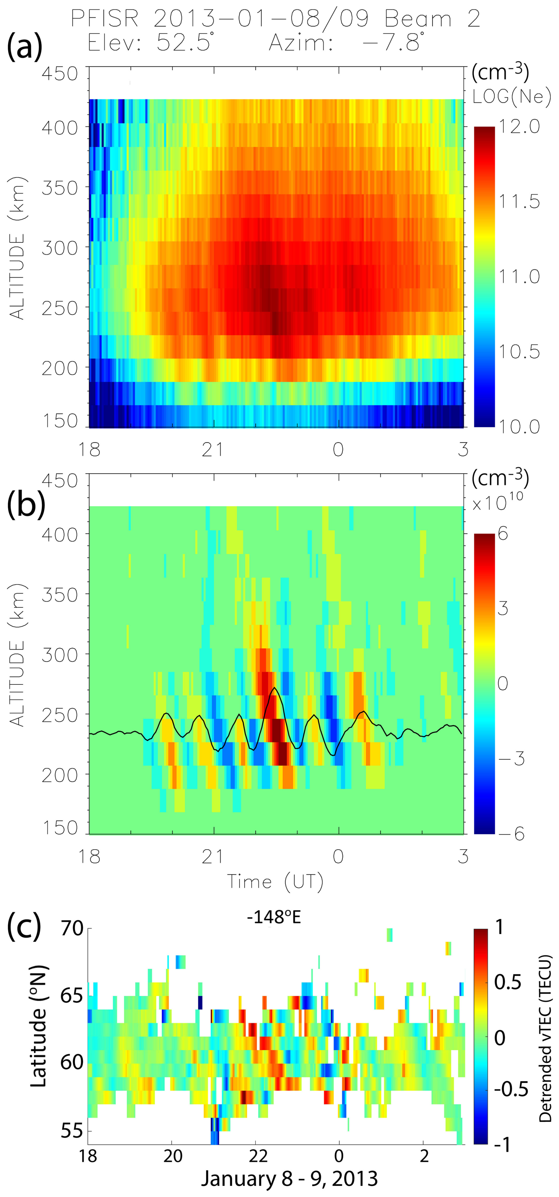
Figure 2 (a) Ionospheric density observed by the PFISR beam 2 and (b) detrended using a 33-point wide Savitzky–Golay filter. (c) The detrended GNSS vTEC mapped at latitude bins along the longitude of PFISR.

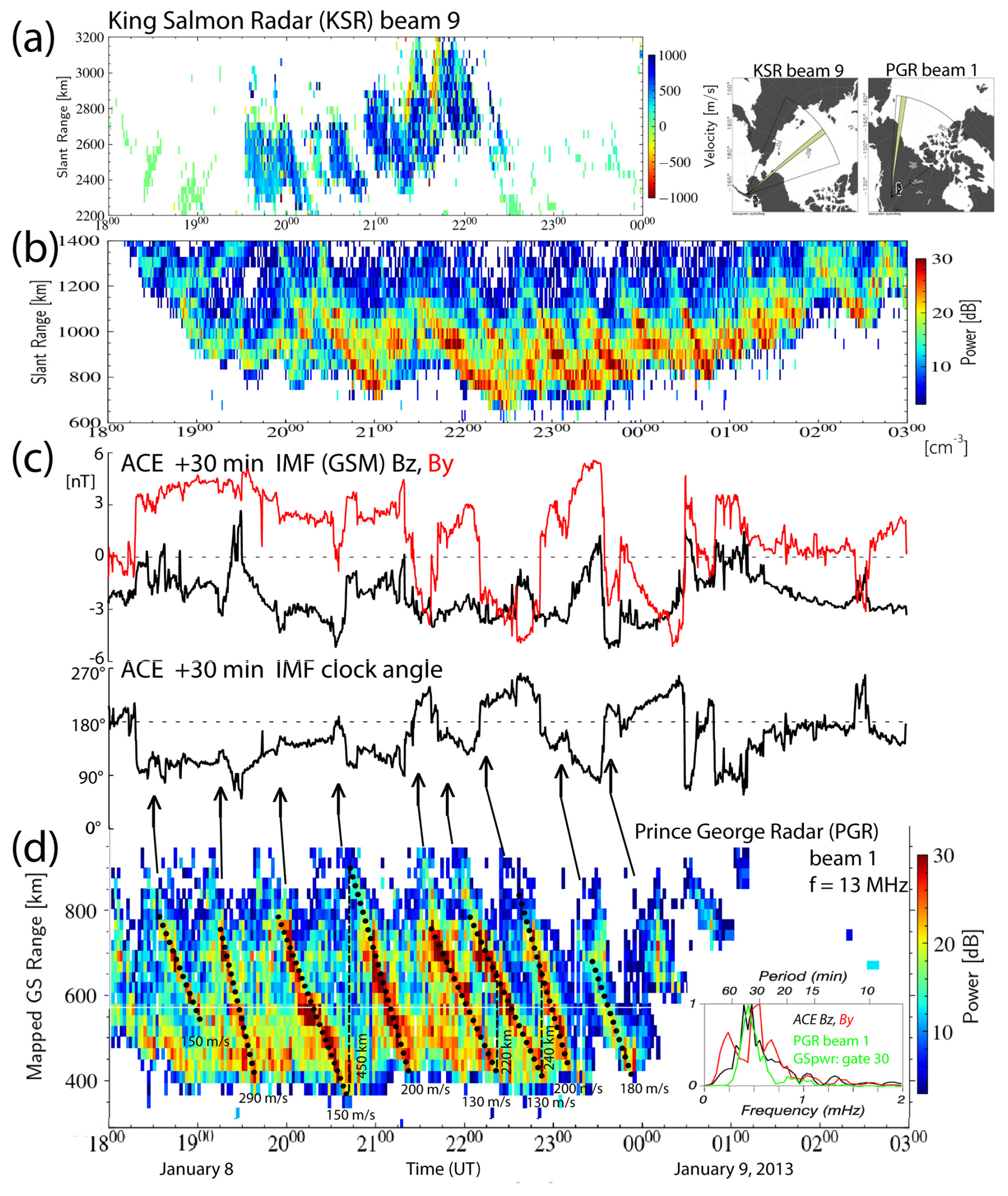
Figure 3 (a) The line-of-sight velocities and (b) the sea scatter power as a function of the slant range observed by the KSR beam 9. (c) The time-shifted time series of the IMF B_z and B_y as well as the IMF clock angle observed by ACE spacecraft. (d) The mapped ground scatter power observed by the PGR beam 1. The arrows indicate southward turning of the IMF. Normalized FFT spectra of the detrended IMF B_z, B_y, and Prince George radar ground scatter power (beam 1, gate 30, mapped GS range 730 km) are shown in the inset. The estimated TID wavelengths and phase velocities are shown.

3.1 Event of 8/9 January 2013

In the period from 8 to 15 January the PFISR beams scanned electron densities, N_e (cm⁻³), at altitudes from 150 to 500 km. In the detrended TEC maps over Alaska (https://aer-nc-web.nict.go.jp/GPS/GLOBAL/MAP/2013/008/index.html, last access: 11 July 2025) the equatorward-propagating TIDs were observed each day during the daytime hours when the PFISR density data show signatures of the downward-propagating phase of TIDs. Figure 2a shows N_e in logarithmic scale as a function of altitude observed by radar beam 2 at a temporal resolution of 3 min between 18:00 and 03:00 UT (09:00 and 18:00 LT) on 8–9 January 2013. The downward-propagating phase of TIDs is readily seen superposed on the background of high daytime densities. To remove the background and highlight the TIDs with periods >40 min the time series for each altitude are detrended using a 33-point wide Savitzky–Golay filter (fourth degree, second order) (Fig. 2b). To show the equatorward propagation of the TIDs across Alaska, Fig. 2c shows the detrended GNSS vTEC mapped at latitude bins along the longitude of the PFISR.

The geomagnetic activity on 8 January was low, with the Kp index at ≤1 except for a peak of 3 in the last 3-hourly interval caused by a substorm that occurred in the European sector. The northernmost magnetometer in Alaska in Barrow (now Utqiaġvik) observed the north–south x-component magnetic field perturbation of ∼230 nT at 17:10 UT (see Fig. S1 in the Supplement), indicating the westward electrojet. At this time, the IMF was pointing dawnward (B_y<0) and eastward flows (see Fig. S2a in the Supplement) in the dawn convection cell corresponded to the westward electrojet sensed in Barrow. After 18:00 UT, as the IMF B_y reversed to duskward (Fig. 2c), the convection cells receded further poleward of Alaska, and the convection pattern become dominated by the dusk cell (see Fig. S2b in the Supplement). At this time, the distant westward electrojet over the Beaufort Sea could no longer be detected by magnetometers.

The King Salmon Radar (KSR) beam 9 pointing northwest over the East Siberian Sea observed positive (towards the radar) line-of-sight (LoS) velocities indicating quasiperiodic (20–50 min) pulsed ionospheric flows (PIFs; Fig. 3a) in the dawn convection cell. At near ranges, the KSR observed enhancements in the sea scatter power (Fig. 3b) caused by a series of equatorward-propagating TIDs. The Prince George Radar (PGR) beam 1 also observed the TIDs in the ground scatter power with periods similar to those of PIFs and the TIDs observed by PFISR (Fig. 2). To show the actual TID location in the ionosphere, instead of the slant range the ground scatter range mapping (Bristow et al., 1994; Frissell et al., 2014) is applied in Fig. 3d. Projected to the direction of beam 1, the estimated TID wavelengths ranged between ∼200 and 500 km and phase velocities between ∼100 and 300 m s⁻¹.

The IMF southward turnings are expected to modulate the reconnection rate at the magnetopause, leading to intensifications of the ionospheric convection/currents in the cusp footprint. One of the convection enhancements can be viewed in Fig. S2b in the Supplement. Pulsed ionospheric flows are known to be associated with particle precipitation in poleward-moving auroral forms (Rae et al., 2004). In the cusp, particle precipitation and Joule heating can be comparable energy sources for AGWs/TIDs (Nykiel et al., 2024). The time series of the ACE IMF B_y and B_z, as well as the clock angle (B_z, B_y) counted from the geomagnetic north, with 180° (dotted line) indicating southward turnings of the IMF, are shown time-shifted in Fig. 3c. Normalized fast Fourier transform (FFT) spectra of the detrended IMF B_z, B_y, and the Prince George radar ground scatter power (beam 1, gate 30, mapped GS range 730 km) are shown in the inset in Fig. 3d. The spectra of the IMF B_z and the Prince George radar ground scatter power are very similar, thus providing evidence that the generation of TIDs was driven by solar wind coupling to the dayside magnetosphere. The clock angle controls the reconnection rate at the magnetopause (Milan et al., 2012). The TIDs can be approximately associated with southward IMF turnings (positive deflections of the clock angle values towards 180° marked by arrows in Fig. 3). Of course, this is an approximate correspondence. The IMF observed by ACE does not exactly represent the IMF impacting the dayside magnetopause. It would require at least a spacecraft in front of the bow shock to monitor the IMF (e.g., Prikryl et al., 2002). But the observations of pulsed ionospheric flows (PIFs) and corresponding TIDs points to sources of these TIDs in the high-latitude ionosphere poleward of Alaska. Prikryl et al. (2005; their Fig. 2) showed that the observed TID propagation times, horizontal wavelengths, and phase velocities deduced from the ground scatter are consistent with the results of ray tracing of the gravity wave energy from an ionospheric source.

While we focused here on 8/9 January, on each day during the PFISR experiment from 8 to 15 January the solar wind–M-I-T coupling that modulated PIFs in the ionospheric cusp footprint poleward of Alaska launched TIDs that were observed by PFISR, as well as in the GNSS vTEC maps. Similarly, in the European sector, dayside TIDs propagating equatorward from their sources in the cusp over Svalbard were also observed. This can be viewed in Fig. S3 in the Supplement, and it is consistent with previous studies of PIFs in the ionospheric cusp resulting in TIDs (Prikryl et al., 2005, 2022).

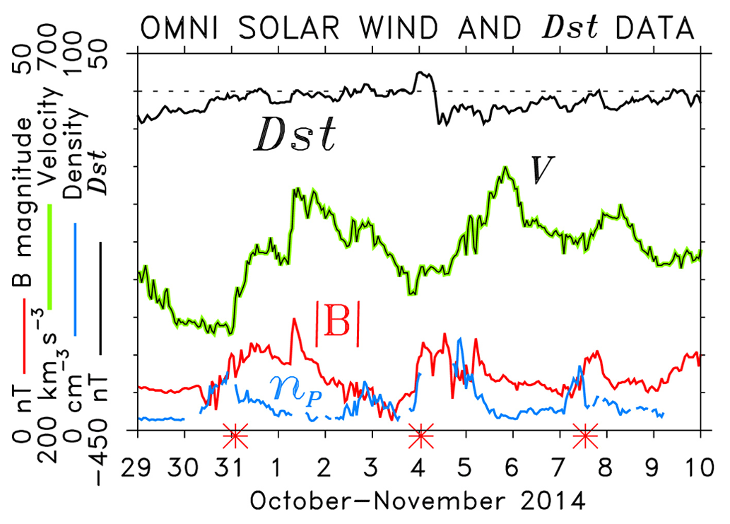
Figure 4 The OMNI solar wind velocity V, magnetic field magnitude $\left|B\right|$, and proton density n_p, showing three HSSs/CIRs on 31 October and 4 and 7 November, are marked by red asterisks on the time axis. The ring current Dst index is also shown.

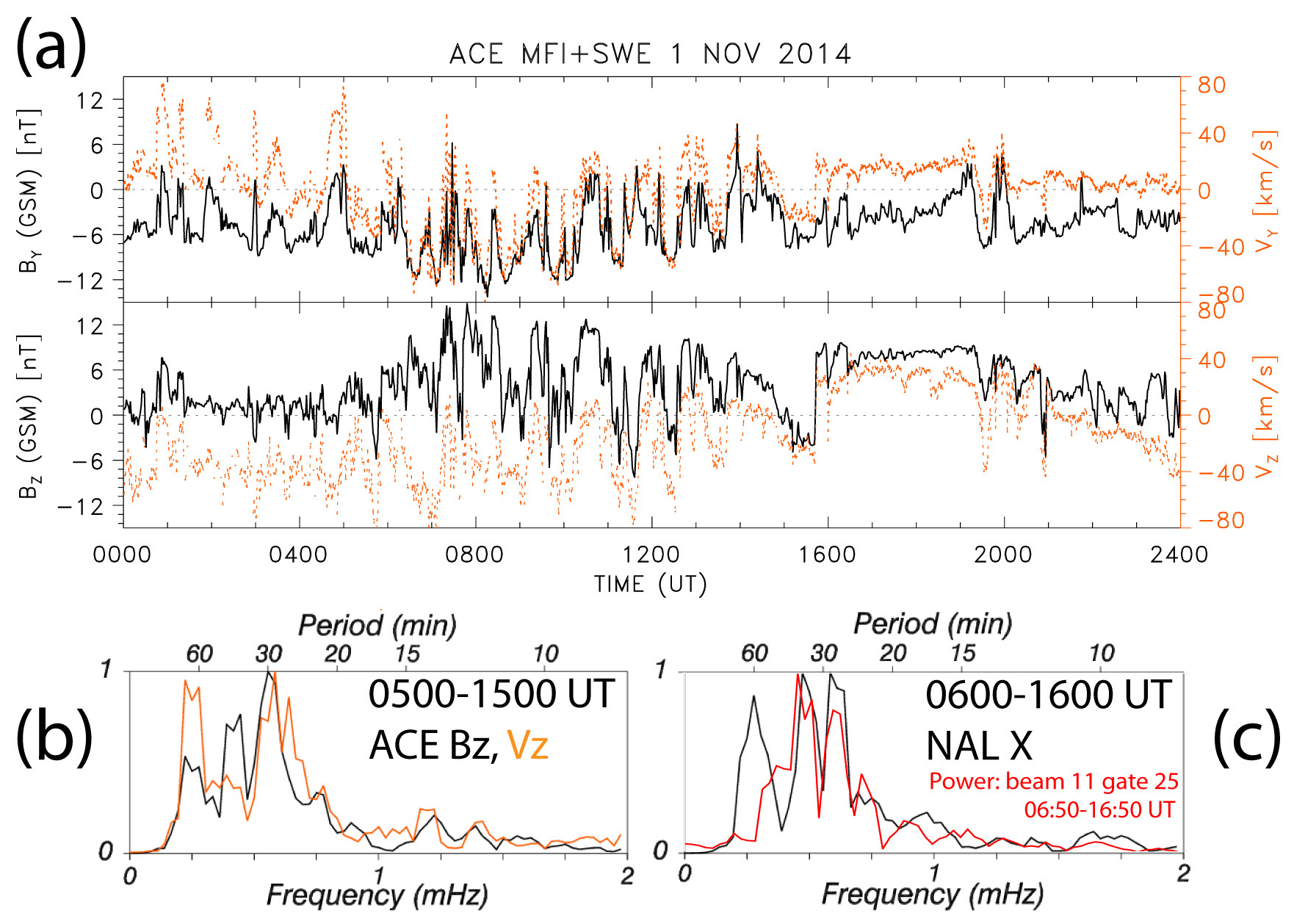
Figure 5 (a) The components of the magnetic field and solar wind velocity observed by ACE, (b) the FFT spectra of the detrended time series of IMF B_z and solar velocity V_z, and (c) the FFT spectra of the time series of the x component of ground magnetic field perturbations in Ny-Ålesund (NAL) and the Hankasalmi radar ground scatter power (beam 11, gate 25, slant range 1305 km).

3.2 Events of 1 and 4–5 November 2014

Figure 4 shows the solar wind data indicating arrivals of HSS/CIRs marked by asterisks. The second one triggered a minor geomagnetic storm, with the Dst index (Gonzalez et al., 1994) reaching a maximum negative value of −44 nT on 4 November. Solar wind Alfvén waves permeate HSSs and, along with CIRs, are highly geoeffective when IMF B_z<0 (Tsurutani and Gonzalez, 1987; Tsurutani et al., 1995, 2006). On 1 and 5 November 2014, the solar wind Alfvén waves are characterized by the Walén relation between velocity V and magnetic field B (Yang et al., 2020). The components of the corresponding components of the magnetic field (B_y and B_z) and velocity (V_y and V_z) observed by ACE are correlated (Fig. 5a), which is a signature of solar wind Alfvén waves. For 5 November, this can be viewed in Fig. S4a in the Supplement.

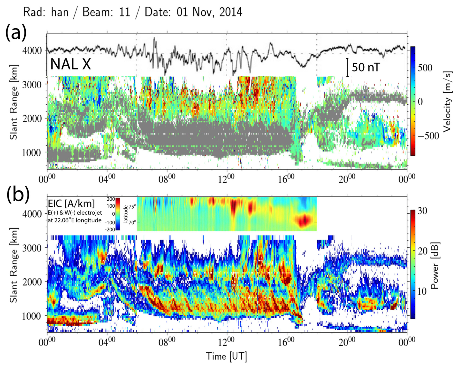
Figure 6 (a) The line-of-sight (LoS) velocity and (b) the radar scatter power (ground scatter power shown in gray in the velocity plot) observed by the Hankasalmi radar beam 11 on 1 November 2014. The x component of the ground magnetic field perturbations in Ny-Ålesund (NAL) is superposed, representing the fluctuations of ionospheric currents modulated by solar wind Alfvén waves. 1D equivalent current estimates that use all IMAGE magnetometers are also superposed.

Figure 7 The same as Fig. 6 but for 5 November 2014.

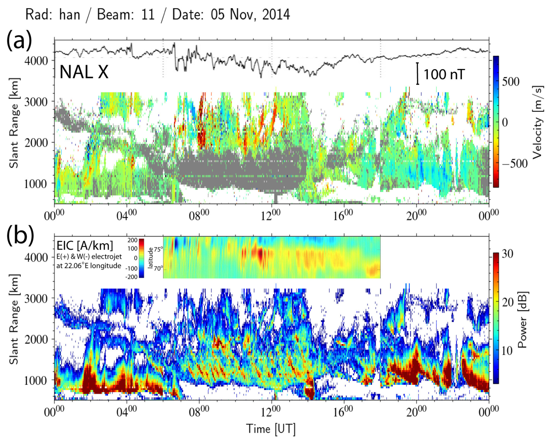
In the European sector, the SuperDARN Hankasalmi radar observed PIFs in the cusp over Svalbard and equatorward-propagating TIDs, which were also observed in the detrended vTEC. Figures 6 and 7 show the ionospheric LoS velocities and the radar scatter power (ground scatter shown in gray in the velocity plot) observed by radar beam 11 on 1 and 5 November, respectively. The radar ground scatter (Figs. 6b and 7b) at ranges between 1000 and 1800 km shows tilted bands due to equatorward-propagating TIDs. Applying the ground scatter mapping method (as already discussed in Sect. 3.1), the estimated MSTID wavelengths ranged between ∼100 and 500 km and phase velocities between ∼100 and 300 m s⁻¹ (Fig. S5a and b in the Supplement).

The ground magnetic field perturbations of the x component observed in Ny-Ålesund (NAL; https://space.fmi.fi/image/www/index.php, last access: 11 July 2025) and 1D equivalent current estimates that use all IMAGE magnetometers are superposed. The radar observed a series of intensifications of the negative (away from the radar) LoS velocities (PIFs) at ranges greater than ∼2000 km on the dayside, starting at ∼07:00 UT with the onset of ionospheric current fluctuations sensed by the NAL magnetometer. The solar wind Alfvén waves modulated the dayside ionospheric currents launching AGWs driving the equatorward-propagating TIDs observed in the radar ground scatter at ranges below ∼2000 km. For 1 November, Fig. 5b and c show the FFT spectra of detrended time series of IMF B_z, solar velocity V_z, the NAL x component, and the Hankasalmi radar ground scatter power (beam 11, gate 25, slant range 1305 km) displaying peaks at similar frequencies/periods. For 5 November, the FFT spectra can be viewed in Fig. S4b and c in the Supplement.

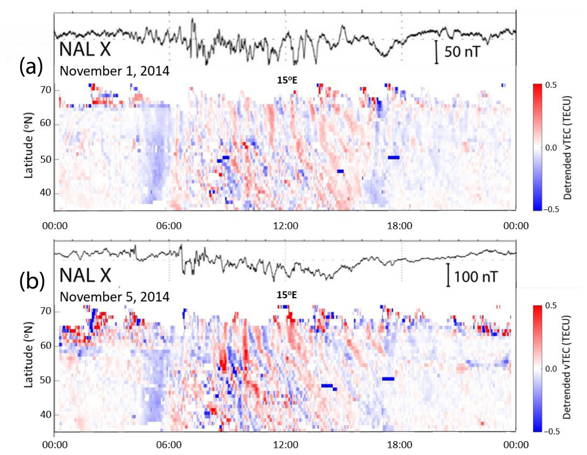
Figure 8 The detrended vTEC mapped along longitude of 15° E on (a) 1 November and (b) 5 November 2014. The x component of the ground magnetic field perturbations in Ny-Ålesund (NAL) is superposed.

Figure 8a and b show the TIDs observed in the detrended vTEC as alternating positive and negative anomalies mapped along longitude of 15° E on 1 and 5 November, respectively. The equatorward-propagating TIDs were observed at midlatitudes, but it is difficult to estimate their propagation speeds as they appear to have been disrupted due to interference with TIDs from tropospheric sources moving eastward to southeastward that are discussed in Sect. 4.

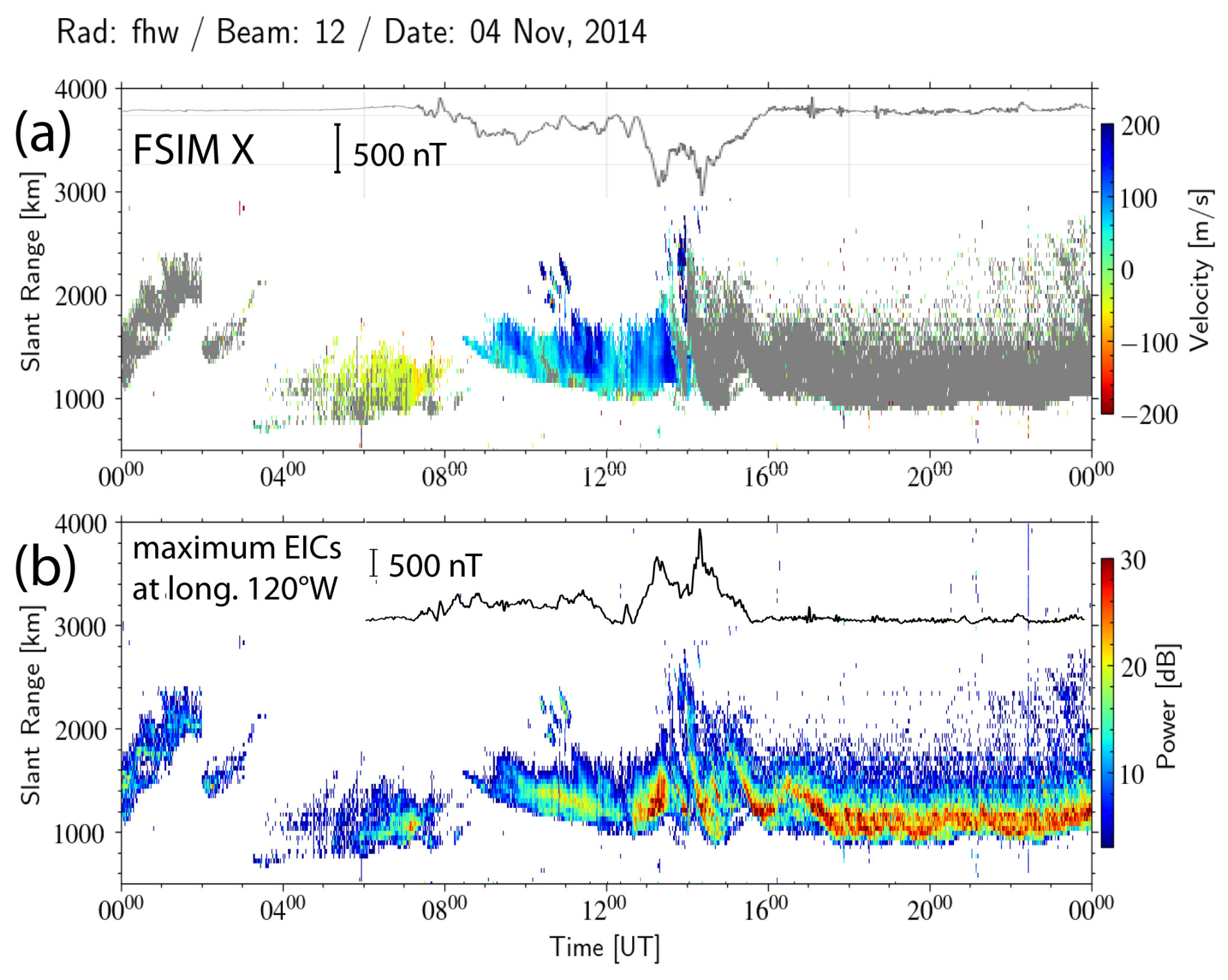
Figure 9 (a) The line-of-sight (LoS) velocity and (b) the radar scatter power (ground scatter power shown in gray in the velocity plot) observed by the Fort Hays West radar beam 12 on 4 November 2014. The x component of the ground magnetic field perturbations in Fort Simpson (FSIM) and the maximum EICs at longitude 120° W are superposed.

The arrival of the HSS/CIR on 4 November triggered a minor geomagnetic storm. Similar to cases reported previously (Prikryl et al., 2022), intense ionospheric currents in the North American sector auroral zone launched TIDs that were observed by the midlatitude SuperDARN radars and the detrended TEC. Before 04:00 UT at a radar frequency at of 11.5 MHz, the Fort Hays West (FHW) midlatitude radar beam 12 looking northwest over central Canada observed the ionospheric scatter, showing enhancements in the positive LoS velocities (toward the radar; Fig. 9a) due to fluctuating eastward ionospheric flows at the equatorward edge of an expanded dawn convection cell associated with the fluctuating westward electrojet. The ionospheric currents were sensed by magnetometers, including one in Fort Simpson (FSIM; http://www.carisma.ca/, last access: 11 July 2025). The x component of the ground magnetic field and time series of the latitudinal maxima in EICs at the longitude of 120° W are superposed. After 14:00 UT, when the radar frequency was set to 15 MHz, the HF propagation allowed observing TIDs in the ground scatter. The ground scatter slant ranges between 1000 and 3000 km correspond to the mapped ground scatter ranges between 200 and 1200 km.

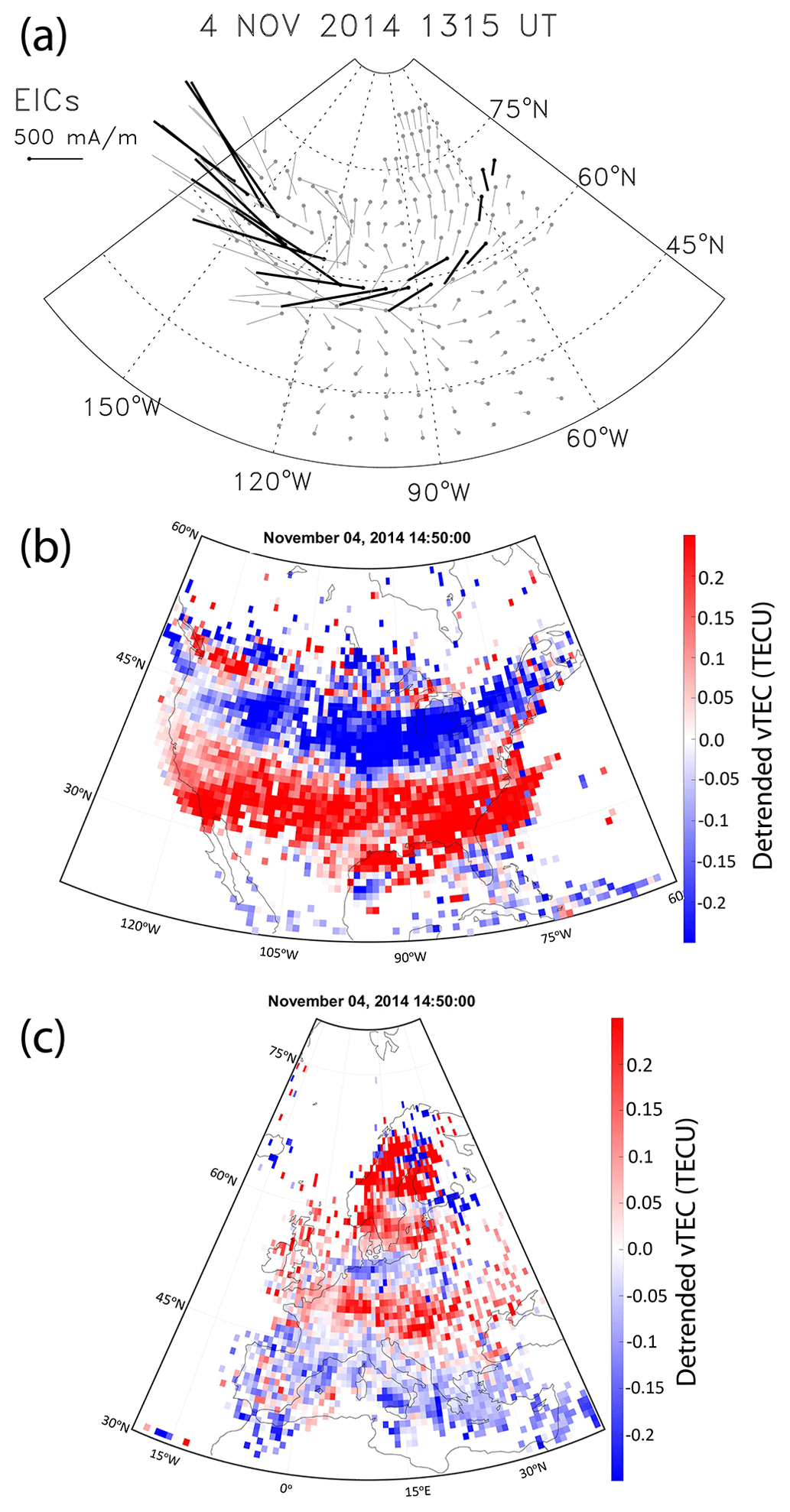
Figure 10 (a) The intensification of the westward electrojet over North America and LSTIDs in the detrended vTEC maps over (b) North America and (c) Europe.

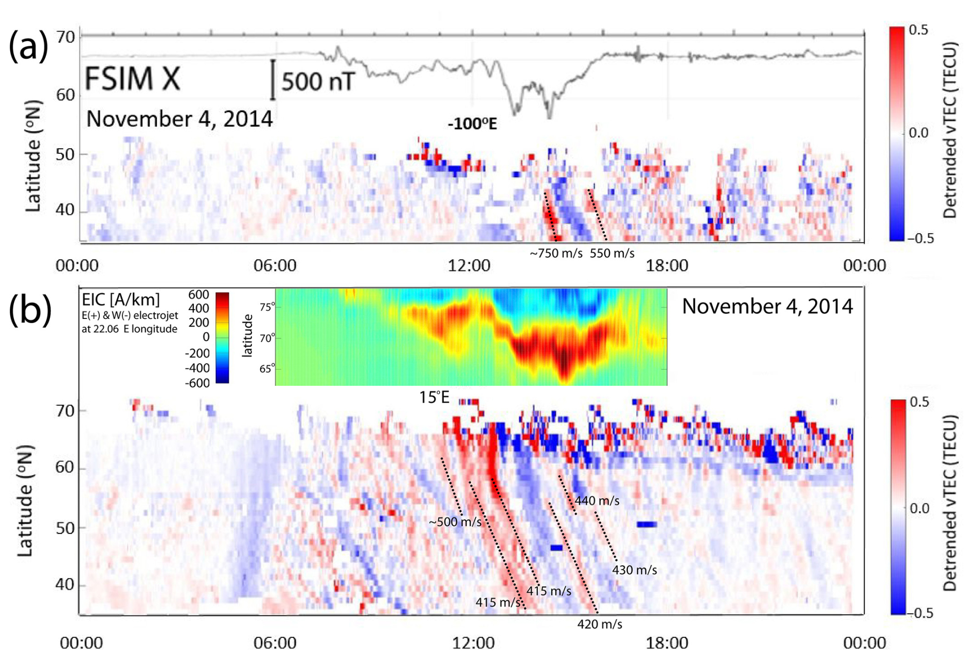
Figure 11 The detrended vTEC mapped along longitude of (a) 100° W and (b) 15° E on 4 November 2014. The x component of the ground magnetic field in Fort Simpson (FSIM) and 1D equivalent current estimates over Scandinavia are superposed.

Two major intensifications of the westward electrojet at ∼13:10 and 14:10 UT (Fig. 9b) launched LSTIDs observed in the ground scatter starting at ∼14:00 and 15:00 UT. The mapped EICs in Fig. 10a show the first major intensification of the westward electrojet (the EIC maxima at each longitude are highlighted) that was followed by the second intensification 1 h later (Fig. 9b). They launched equatorward-propagating LSTIDs (wavelength greater than 1000 km) observed in the detrended vTEC maps (Fig. 10b). Figure 11a shows the LSTIDs between 13:00 and 16:00 UT in the detrended vTEC mapped along longitude of 100° W in the North American sector. The approximate equatorward propagation speeds were between 500 and 800 m s⁻¹.

In the European sector, during the most disturbed time following the HSS/CIR arrival on 4 November, the dayside auroral oval expanded down to latitude ∼63° N. Figure 11b shows the equivalent ionospheric currents estimated from the IMAGE magnetometers. LSTIDs (Fig. 10c) that were launched by intensifications of the east electrojet were observed propagating equatorward at speeds between 400 and 500 m s⁻¹ in midlatitudes are mapped along longitude of 15° W between 11:00 and 18:00 UT (Fig. 11b).

In summary, the cases discussed in Sect. 3.1 and 3.2 highlight the importance of solar wind coupling to the M-I-T system, particularly on the dayside, in the generation of AGWs/TIDs. The fluctuations of the IMF, sometimes Alfvénic, modulate PIFs and ionospheric currents in the cusp, launching GW/TIDs.

4 AGWs/TIDs originating from sources in the troposphere

MSTIDs caused by GWs with periods of 10–40 min propagating obliquely upward in the thermosphere/ionosphere have been studied using the multifrequency and multipoint continuous HF Doppler sounding system located in the western part of Czechia (Chum et al., 2021). The 2D propagation analysis of the HF Doppler sounders data is applied to available signals to exclude data gaps and to select time intervals in which the phase shifts/time delays between signals corresponding to different sounding paths (transmitter–receiver pairs) were approximately constant.

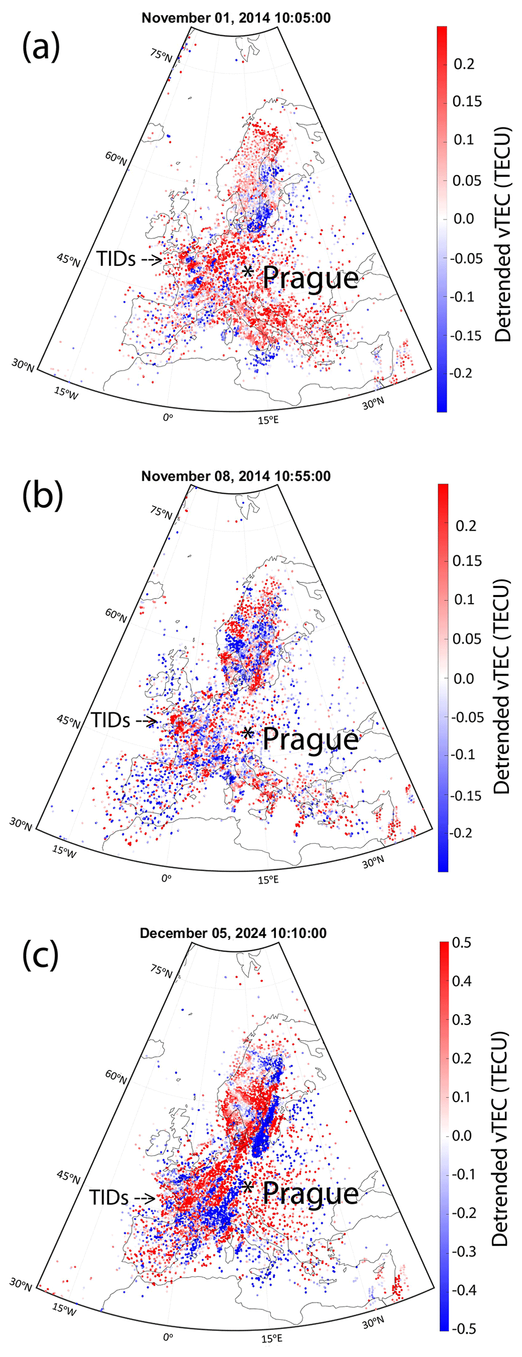
Figure 12 The detrended vTEC maps on (a) 1 November 2014, (b) 8 November 2014, and (c) 5 December 2024.

The observed azimuths depend on season, with southeastward propagation more likely in winter months, suggesting that cold-season low-pressure systems in the northeast Atlantic are sources of the GWs, which supports previously published results (Azeem et al., 2018) and points to the winter jet stream as a likely source of GWs. In this section we examine such cases and trace TIDs in the detrended GNSS TEC maps (Fig. 12) and observed by the HF Doppler sounders propagating eastward to southeastward from intensifying low-pressure weather systems over the eastern Atlantic. The animated TEC maps can be viewed in the Supplement Video, which also shows the equatorward-propagating TIDs that originated at high latitudes as discussed in Sect. 3.

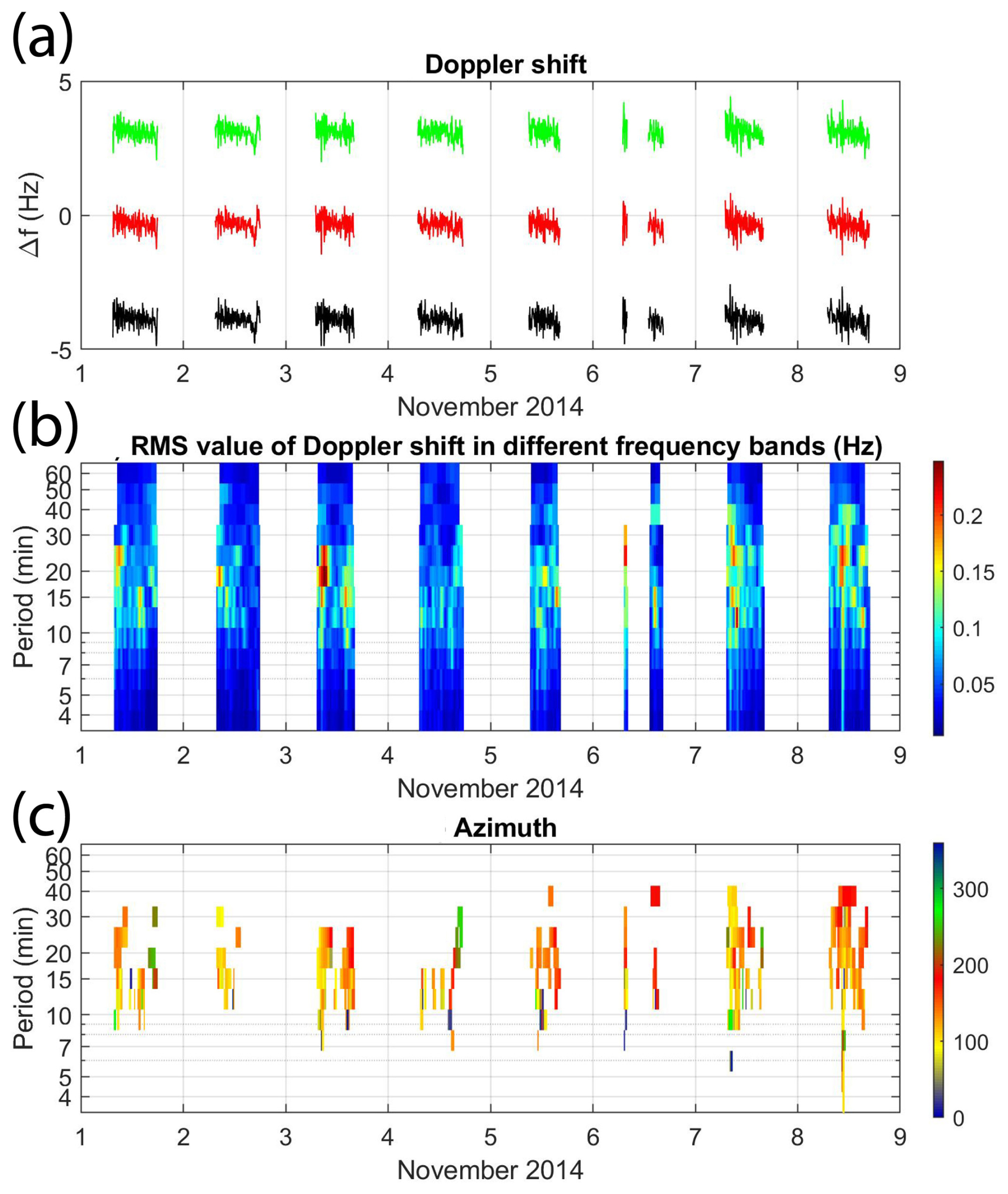
Figure 13 (a) Doppler shift frequencies of spectral density maxima for individual transmitter–receiver pairs (including artificial offsets) from x to y. (b) Dynamic spectra (periodograms) of Doppler shift signals and (c) the propagation azimuth of waves, displayed as a function of period and time for 1–8 November 2014.

4.1 Events of 1–8 November 2014

Spectral and propagation analysis for all available 7.04 MHz signals from 1 to 8 November 2014 was performed (Fig. 13). Only daytime values are available because the critical frequency foF2 is too low at night (most of the nights are also not available at 4.65 MHz). On 6 November enhanced noise (electromagnetic interference) prevented reliable analysis for a substantial part of the day. Figure 13b shows dynamic spectra (periodograms) of a Doppler shift signal obtained as the average of the maxima of three power spectral densities corresponding to three different transmitter–receiver pairs (Sect. 2) shown in Fig. 13a (including artificial offsets). The observed periods (Fig. 13b) range from 10 to about 40 min. The propagation azimuths (Fig. 13c) were mostly from 100 to about 160° (waves propagating southeastward). In all cases, the azimuth is only plotted if the averaged Doppler fluctuations exceeded 0.12 Hz, the estimate of the uncertainty of the azimuth is less than 10°, and the estimate of uncertainty in velocity is less than 10 %. The phase velocities fluctuated typically between 100 and 200 m s⁻¹. Figure 14 shows the analysis results on an expanded timescale to better see the TID characteristics for 8 November.

Figure 14 The same as Fig. 12 but expanded for 8 November 2014.

During the period from 1 to 8 November 2014, the southeastward-propagating MSTIDs were observed by the HF sounders and detrended vTEC. Low-pressure systems deepening over the northeastern Atlantic, shown in the surface pressure analysis charts (https://www.wetter3.de/archiv_ukmet_dt.html, last access: 11 July 2025), were likely sources of these MSTIDs propagating eastward to southeastward, as observed in the detrended vTEC maps (indicated by arrows in Fig. 12a, b) on 1 and 8 November 2014. At the same time, the vTEC maps on both days also reveal equatorward-propagating TIDs at latitudes down to ∼50° N that originated in the cusp ionospheric footprint over Svalbard, as already discussed in Sect. 3.2.

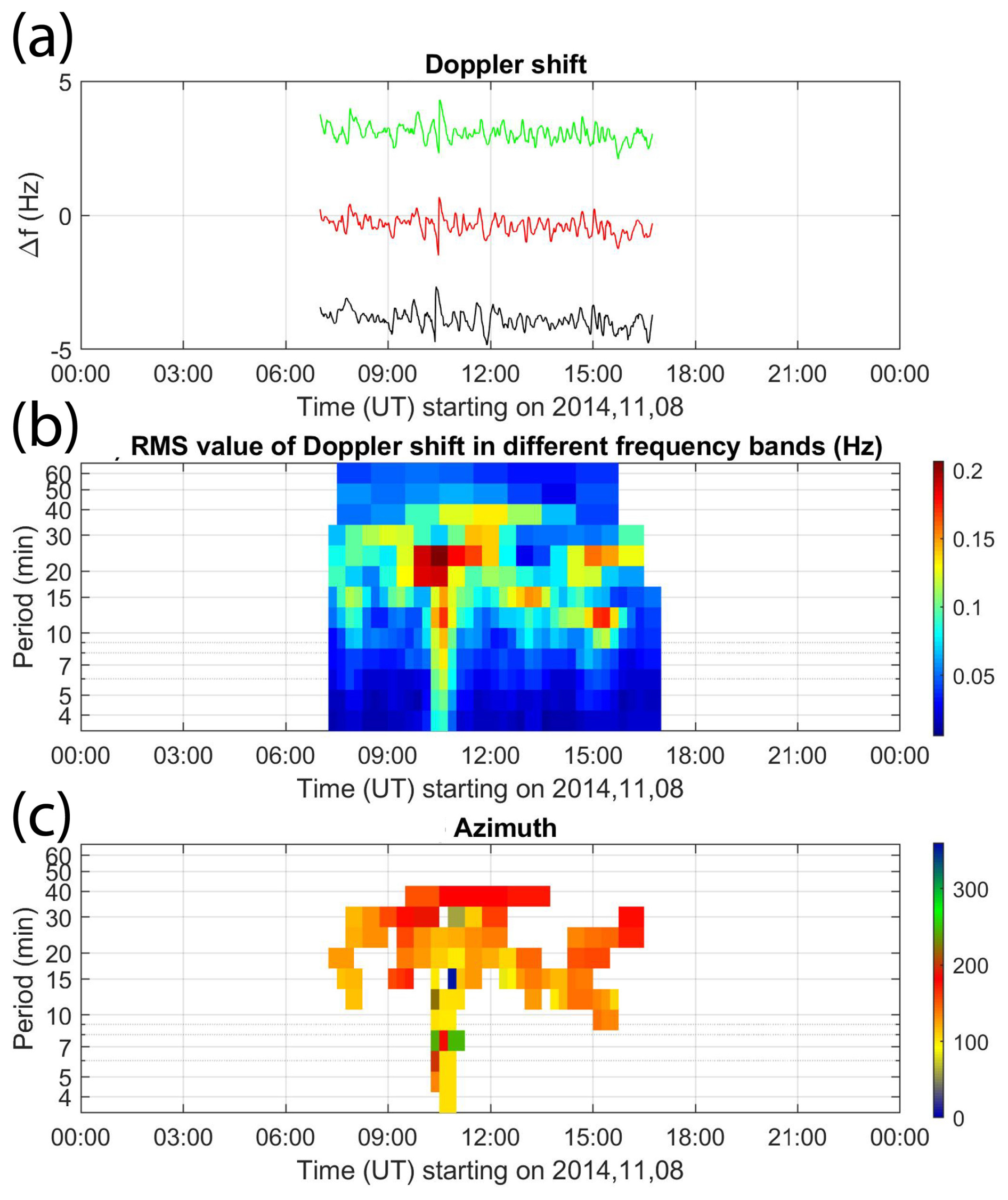
The Doppler shift frequencies (Fig. 14a) recorded at a frequency of 7.04 MHz on 8 November 2014 show the temporal evolution of the power spectral densities (color-coded arbitrary units) of received signals that correspond to three different transmitter–receiver pairs. There was enhanced noise due to the electromagnetic interference on 8 November from about 09:30 to 12:30 UT. The straight horizontal line in the upper signal trace in the spectrogram corresponds to a ground wave from one of the transmitters, located only ∼7 km from the receiver. The middle and bottom signal traces in the spectrogram correspond to the other two transmitters. As described in more detail in Sect. 2.2, the use of well-correlated signals at two or three different frequencies makes it possible to determine a 3D phase velocity vector. The results that are summarized in Table S1 in the Supplement separately for the observation at frequencies of 4.65 and 7.04 MHz show mostly similar values of horizontal velocities (ranging from ∼100 to 200 m s⁻¹) and azimuths (ranging from ∼90 to 145°).

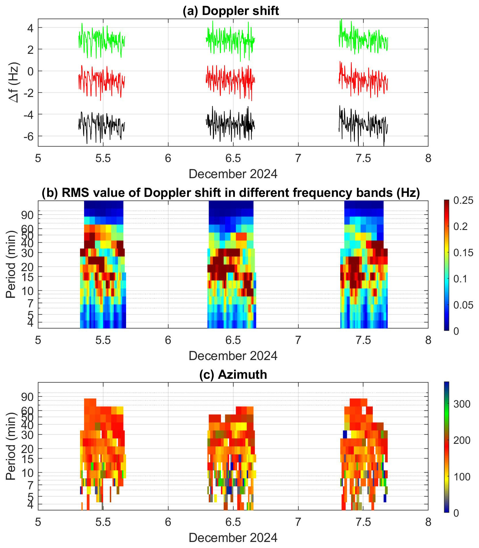
Figure 15 (a) Doppler shift frequencies of spectral density maxima for individual transmitter–receiver pairs (including artificial offsets) from x to y. (b) Dynamic spectra (periodograms) of Doppler shift signals and (c) the propagation azimuth of waves, displayed as a function of period and time for 5–7 December 2024.

4.2 Events of 5–7 December 2024

Similarly to events discussed in Sect. 4.1, low-pressure systems deepening over the northeastern Atlantic on 5–7 December were likely sources of GWs driving the observed southeastward-propagating MSTIDs (Fig. 12c). To further support the results in Sect. 4.1 we analyzed these recent events recorded at 4.65 and 7.04 MHz. Due to the critical frequency of the ionosphere, 4.65 MHz allows obtaining longer time intervals with usable signals but with smaller amplitudes. The signals at 7.04 MHz are reflected from higher altitudes where the amplitudes are larger. The results of the spectral and propagation analysis for all available 7.03 MHz signals for 5–7 December 2024 are shown in Fig. 15. Figure 15b shows dynamic spectra of the Doppler shift signal obtained as the average of the frequencies corresponding to the maxima of the three power spectral densities for the three different transmitter–receiver pairs shown in Fig. 15a (including artificial offsets, which were removed before the spectral and propagation analysis). The observed periods of TIDs/GWs (Fig. 15b) range from a few minutes up to 1 h. The propagation azimuths (Fig. 15c) were mostly around 140°. (southeastward), and phase velocities fluctuated typically between 150 and 290 m s⁻¹.

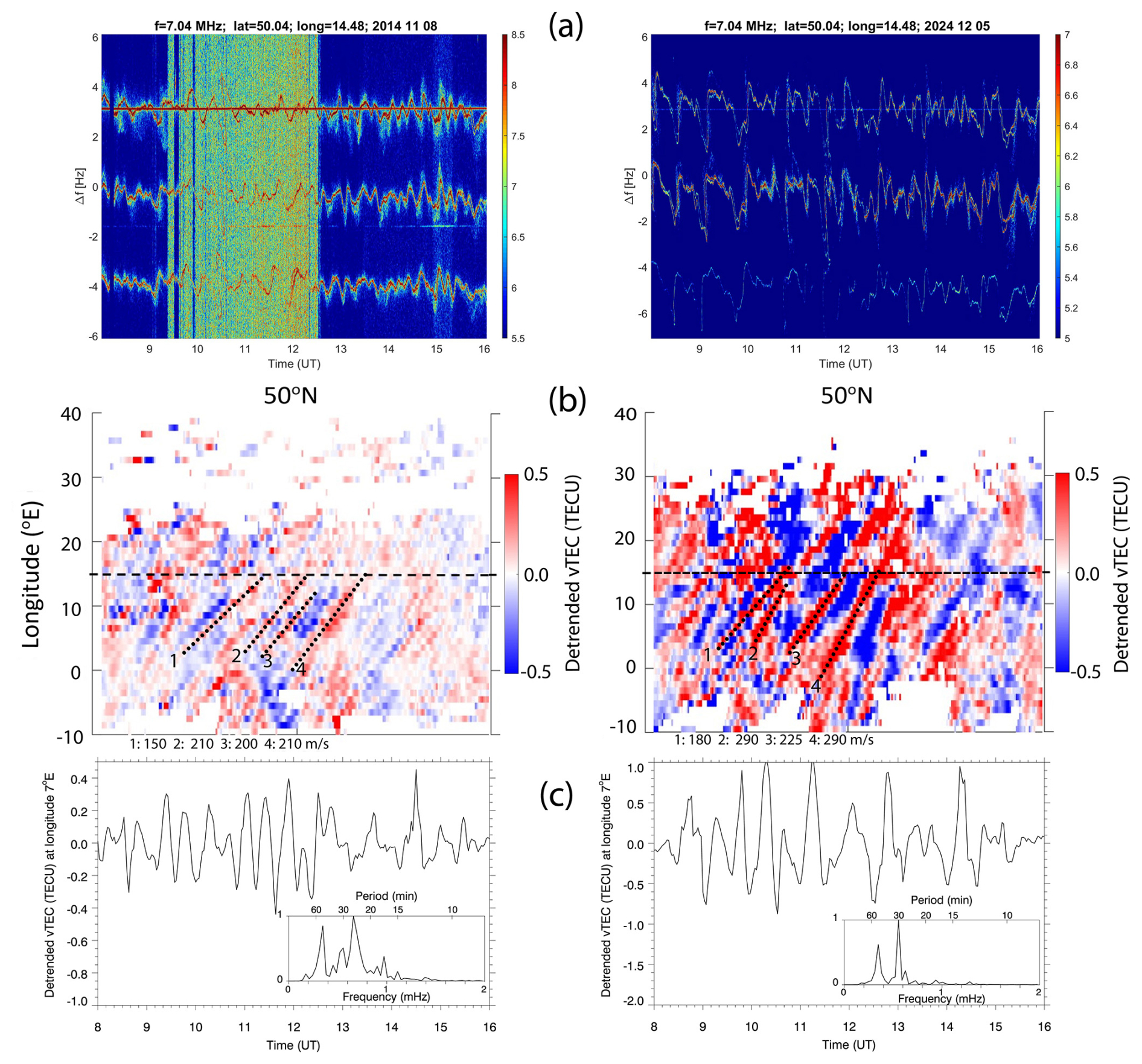
Figure 16 (a) The Doppler shift spectrogram recorded at a frequency of 7.04 MHz on 8 November 2014 and 5 December 2024. (b) The detrended vTEC mapped along latitude of 50° N. The dashed line shows the longitude of Prague. The approximate eastward velocities of TIDs shown as dotted lines are estimated. (c) The detrended vTEC time series at longitude of 7° E and the normalized FFT spectra.

4.3 Comparison between TIDs observed in the detrended vTEC maps and by the HF Doppler sounding system

The Doppler shift spectrograms recorded at a frequency of 7.04 MHz on 8 November 2014 and 5 December 2024 are shown in Fig. 16a (top panels). In Fig. 16b (middle panels), the detrended vTEC mapped along the latitude of 50° shows eastward-propagating TIDs towards the longitude of the HF sounding system with estimated approximate velocities shown. The bottom panels (Fig. 16c) show time series of the detrended vTEC at longitude of 7° E with the normalized FFT spectra shown in the insets.

In November 2014, the amplitudes of MSTIDs observed in the detrended vTEC and by the HF Doppler sounder were relatively small, and the coverage by GNSS receivers at longitudes greater than 10° E was sparse. In contrast, in December 2024, the GNSS coverage significantly improved, and the amplitudes of MSTIDs observed both in the vTEC and by HF Doppler sounder were much larger.

While it is difficult to compare in detail the results obtained by these two very different techniques (one based on the global mapping of vTEC using the thin shell approximation at 350 km altitude and the other local measurements dependent on the HF propagation and the critical frequency for reflection altitude), the phase velocities (Fig. 16b) and periods (Fig. 16c) of TIDs estimated from the detrended vTEC are similar to those obtained by the HF Doppler sounder as discussed in Sect. 4.1 and 4.2 (Figs. 14 and 15).

More cases of eastward- to southeastward-propagating MSTIDs observed by the HF Doppler sounder and in the detrended vTEC observed in 2014 on 1, 3, and 7 November (see Figs. S6–S8 in the Supplement), 22 and 24 November, 9–10 December, and 24 December were also associated with intense low-pressure systems in the northeastern Atlantic.

4.4 Physical mechanism of GW generation in the troposphere

While tropospheric convection is a common source of gravity waves (e.g., Azeem, 2021), no deep convection could be identified in the cold fronts of low-pressure systems over the northeastern Atlantic (GIBBS, https://www.ncdc.noaa.gov/gibbs/html/MSG-3/IR/2014-11-01-00, last access: 11 July 2025). Mesoscale gravity waves generated by geostrophic adjustment processes and shear instability have been observed (Uccellini and Koch, 1987; Koch and Dorian, 1988). Plougonven and Zhang (2014) reviewed the current knowledge and understanding of gravity waves near jets and fronts. Plougonven and Teitelbaum (2003; their Fig. 2) showed patterns of alternating bands of convergence and divergence in maps of the divergence of the horizontal wind for the lower stratosphere, which have been interpreted as the signature of inertia-gravity waves propagating upwards above the tropopause. A conceptual model of a common synoptic pattern has been identified with a source of gravity waves near the axis of inflection in the 300 hPa geopotential height field (Koch and O'Handley, 1997; their Fig. 2).

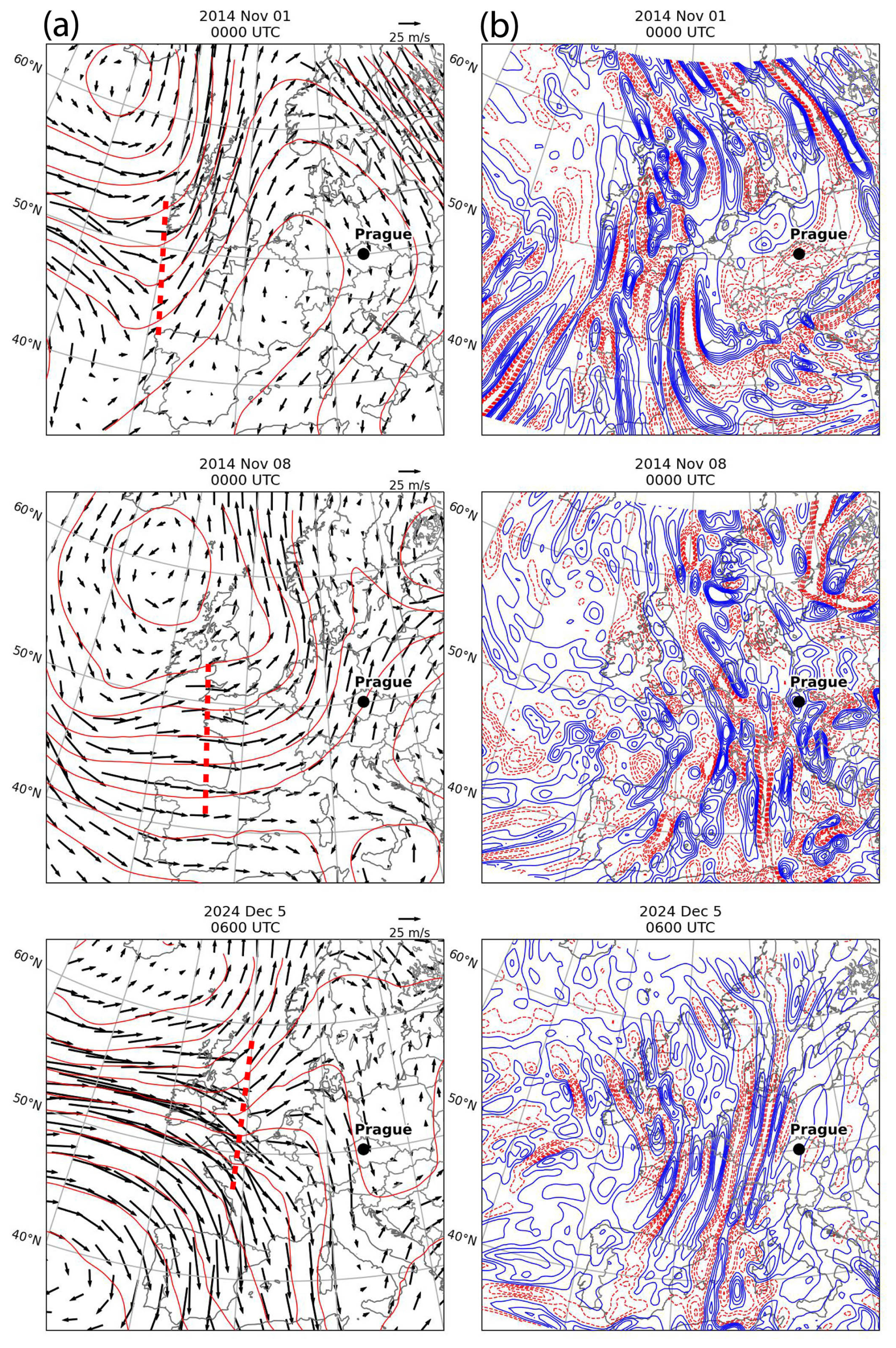
Figure 17 (a) The ERA5 geopotential height (red contours at intervals of 100 m) and horizontal winds (m s⁻¹) at 300 hPa level, with a probable source region of gravity waves indicated by a red dashed line. (b) The ERA5 divergence (positive, solid blue line) of the horizontal wind at 150 hPa level on 1 November, 8 November 2014, and 5 December 2024.

In Sect. 4.1 and 4.2, the cases of MSTIDs on 1 and 8 November 2014 and 5 December 2024 propagating eastward to southeastward observed in the detrended vTEC maps (Fig. 12) and by the HF Doppler sounding system (Figs. 13, 14 and 15) are attributed to sources in the troposphere, namely deepening low-pressure weather systems. This is consistent with the conceptual model referenced above. Using the ERA5 reanalysis (Hersbach et al., 2020), Fig. 17 shows the 300 hPa geopotential height, approximate axis of inflection (a probable source region of gravity waves that is indicated by a red dashed line), and horizontal winds at 300 hPa for the three events in 2014 and 2024. Figure 17b shows the divergence of the horizontal wind at the 150 hPa level. The alternating bands of convergence and divergence are similar to those interpreted by Plougonven and Teitelbaum (2003) as gravity waves propagating to the lower stratosphere. Other cases of MSTIDs on 3 and 7 November can be viewed in Figs. S6 and S7 in the Supplement. Mesoscale GWs propagating eastward and upward into the stratosphere generated by geostrophic adjustment processes and shear instability may be common and could be driving MSTIDs.

5 Discussion

The solar wind–M-I-T coupling is known to modulate the intensity of ionospheric currents, including the auroral electrojets, which in turn launch atmospheric gravity waves, causing TIDs. The cases of dayside equatorward-propagating TIDs were observed with PFISR and SuperDARN and detected in the detrended GNSS vTEC maps. This is consistent with previously published results and interpretations (e.g., Prikryl et al., 2022, and references therein). The dayside TIDs are commonly generated in the ionospheric footprint of the cusp. They were observed every day over Alaska during the PFISR experiment (8–15 January 2013) and in Europe (1–8 November 2014).

In Sect. 3.1, we have shown evidence that even during a geomagnetically very quiet period the TIDs that were observed by PFISR in Alaska can be attributed to sources at high latitudes (Fig. 3). Quasiperiodic intensifications of the high-latitude ionospheric convection that were the source of these TIDs were observed poleward of Alaska over the East Siberian Sea and Beaufort Sea. The ionospheric currents associated with PIFs could not be detected by ground magnetometers, and the Kp index indicated a quiet period. The ionospheric footprint of the cusp where the pulsed ionospheric flows and associated currents are sources of TIDs may be located further poleward of any ground magnetometers. Low geomagnetic activity is often taken as a pretext to dismiss auroral sources of TIDs. Throughout the PFISR experiment from 8 to 15 January 2013 the TIDs that were observed on the dayside resulted from the solar wind–M-I-T coupling that modulated PIFs in the ionospheric cusp footprint poleward of Alaska. It was similar in the European sector.

The importance of solar wind coupling to the M-I-T system, particularly on the dayside, for the generation of AGWs/TIDs (Prikryl et al., 2005) is further highlighted in Sect. 3.2 by cases where solar wind Alfvén waves modulated PIFs and ionospheric currents in the cusp launching AGWs/TIDs.

Regarding TIDs originating from the troposphere, there has been plentiful evidence of neutral atmosphere–ionosphere coupling via atmospheric gravity waves propagating into the upper atmosphere from sources in the lower atmosphere including convective storms (Alexander, 1996). Azeem and Barlage (2018) and Vadas and Azeem (2021) presented cases of convective-storm-generating TIDs, which exhibited partial to full concentric or almost plane-parallel phase fronts. The latter TIDs were generated by an extended squall line (Azeem and Barlage, 2018). However, in the cases discussed in Sect. 4.1 there was no significant convection in the cold fronts that would generate such TIDs. The eastward-propagating MSTIDs observed in the detrended vTEC maps and by the HF originating from a low-pressure sounding system were likely driven by GWs generated by geostrophic adjustment processes and shear instability in the troposphere. Geostrophic adjustment processes (Uccellini and Koch, 1987) generating gravity waves have not been previously considered as sources of TIDs. This is supported by the ERA5 meteorological reanalysis showing the GWs in the lower stratosphere.

The occurrence of eastward-propagating MSTIDs at midlatitudes over Europe is very common in the cold season, and their association with low-pressure systems can be readily seen browsing the archive of detrended TEC maps (https://aer-nc-web.nict.go.jp/GPS/EUROPE/MAP/#2014, last access: 11 July 2025). An assortment of such cases for December 2014 can be viewed in the Supplement in Figs. S9–S13. At the same time, the animations of TEC maps provided in the archive show equatorward-propagating TIDs, including LSTIDs, originating at high latitudes, that are generated by solar wind–M-I-T coupling. Dayside equatorward-propagating TIDs that were observed in the detrended vTEC in Europe (15° E), the US (100° W), and Alaska (148° W) on 5 December 2024 can be viewed in Fig. S14.

In this study, a multi-instrument approach is used to trace/attribute the observed TIDs to sources of AGWs in the upper and lower atmosphere and to identify physical mechanisms. The solar wind coupling to the M-I-T system generates equatorward-propagating TIDs on the dayside even during geomagnetically quiet conditions. This is important, because the auroral sources of TIDs observed during quiet conditions are often not considered. On the other hand, intensifying low-pressure weather systems generate AGWs propagating to the lower stratosphere and beyond, driving TIDs even when there is no significant tropospheric convection. More work needs to be done to better understand such cases, and many aspects of the system as a whole should be considered when determining the source of TIDs, as simple metrics/indices hide critical details.

6 Summary and conclusions

Traveling ionospheric disturbances are observed by radars, Doppler sounders, and the GNSS TEC mapping technique. Medium- to large-scale TIDs propagating equatorward were generated by solar wind coupling to the dayside magnetosphere–ionosphere–thermosphere, modulating ionospheric convection and currents, including auroral electrojets. MSTIDs that were observed over Alaska by the Poker Flat Incoherent Scatter Radar and by two SuperDARN radars are attributed to gravity waves generated in the ionospheric cusp footprint poleward of Alaska even when geomagnetic activity was low. Dayside MSTIDs were observed every day over Alaska during the 7 d PFISR experiment. In another case, following the arrival of a high-speed solar wind stream that triggered a minor geomagnetic storm, major intensifications of the westward electrojet over the North American sector launched LSTIDs observed by a midlatitude SuperDARN radar and in the detrended global TEC maps. In the European sector, the equatorward-propagating TIDs are attributed to solar wind Alfvén waves coupling to the dayside magnetosphere, modulating ionospheric convection and currents in the cusp footprint over Svalbard. On the other hand, the cases of eastward- to southeastward-propagating MSTIDs observed at midlatitudes in the detrended GNSS TEC maps and by the HF Doppler sounders in Czechia originated from low-pressure weather systems intensifying in the northeastern Atlantic. Gravity waves propagating from the troposphere and lower stratosphere were likely generated by geostrophic adjustment processes, which have not been linked to TIDs previously.