Deterministic chaos in modulated multi-cell drifts of localized lower-hybrid oscillations excited by high-frequency waves in the ionosphere

The prominent broad upshifted maximum (BUM) feature in electromagnetic emissions stimulated by powerful high-frequency radio waves in the ionosphere exhibits an exponential spectrum for pump frequencies near a harmonic of the ionospheric electron gyro frequency. Exponential power spectra are a characteristic of deterministic chaos. In the present treatment, a two-fluid model is derived for lower-hybrid (LH) oscillations driven by parametric interaction of the electromagnetic pump field, the electron Bernstein mode, and the upper-hybrid mode, as previously proposed to interpret the BUM. In two-dimensional geometry across the geomagnetic field, LH oscillations localized in cylindrical density depletions are associated with multi-cell plasma drift patterns. The numerical simulations show that topological modulations of the drift can give rise to approximately Lorentzian-shaped pulses in the LH time signal. For parameter values typical of the ionospheric experiments, the exponential power spectrum of the Lorentzian pulses has a slope that is consistent with the slope of the BUM spectrum. The BUM spectral structure is therefore attributed to deterministic chaos in LH dynamics.

1 Introduction

Electromagnetic emissions excited by powerful high-frequency (HF) electromagnetic waves transmitted into the ionosphere from the ground exhibit a rich spectral structure that depends notably on the pump frequency f₀ and its relation to a multiple s of the ionospheric electron gyro frequency f_e (Leyser, 2001). Figure 1 displays the most prominent spectral feature of the stimulated electromagnetic emissions (SEEs), the so-called broad upshifted maximum (BUM), with its spectral maximum at $f_{\mathrm{BUM}}\approx f_{\mathrm{0}}+\mathrm{24}$ kHz. The high-frequency flank of the BUM commonly exhibits an exponential power spectrum, with a constant slope in a semi-logarithmic plot. Also seen in Fig. 1 is a downshifted maximum (DM) at approximately f₀−10 kHz.

As first established in the fluid and nonlinear dynamics communities (Frisch and Morf, 1981; Greenside et al., 1982), exponential power spectra are a characteristic of deterministic chaos. Research on magnetically confined laboratory plasma showed that the associated time evolution consists of intermittent narrow pulses of Lorentzian shape (Pace et al., 2008) that arise because of topological modulations in the plasma drift trajectories in the vicinity of separatrices in the velocity field (Maggs and Morales, 2011, 2012). The topological modulations of a single-cell drift pattern can make pulses of plasma escape or enter the flow cell. In a multi-cell flow pattern, the modulations can make plasma pulses cross separatrices between the cells to switch the flow cell. Numerical simulations of structures formed by a temperature filament in magnetically confined plasma showed that Lorentzian pulses can arise due to the topological modulations of only two modes of coherent drift waves (Shi et al., 2009).

A Lorentzian pulse has the following functional form (Pace et al., 2008; Hornung et al., 2011; Maggs and Morales, 2011):

$$\begin{array}{}\text{(1)}& L\left(t\right)={\displaystyle \frac{A}{\mathrm{1}+(\frac{t-t_{\mathrm{0}}}{\mathit{\tau }}{)}^{\mathrm{2}}}},\end{array}$$

where A is the amplitude of the pulse of width τ centred at time t=t₀. The Fourier transform of L(t) is $\widehat{L}\left(\mathit{\omega }\right)=A\mathit{\tau }\mathit{\pi }{e}^{i\mathit{\omega }{t}_{\mathrm{0}}}{e}^{-\mathit{\omega }\mathit{\tau }}$, such that its power spectrum is

$$\begin{array}{}\text{(2)}& P\left(\mathit{\omega }\right)=A^{\mathrm{2}}{\mathit{\tau }}^{\mathrm{2}}{\mathit{\pi }}^{\mathrm{2}}\exp (-\mathrm{2}\mathit{\omega }\mathit{\tau }).\end{array}$$

A signal time series containing Lorentzian pulses of approximately equal widths τ will thus exhibit an exponential power spectrum $P\left(f\right)\propto \exp (-f/f_{\mathrm{s}})$ with a scaling frequency of $f_{\mathrm{s}}=\mathrm{1}/\left(\mathrm{4}\mathit{\pi }\mathit{\tau }\right)$.

A simplified model of the E×B_g drift associated with lower-hybrid (LH) oscillations localized in cylindrical geometry across the geomagnetic field B_g (where E is the electric field of the LH oscillations) suggested that deterministic chaos could also be excited by HF radio waves in the ionosphere (Leyser, 2021). It was shown that the drift trajectories can be chaotic in the localized multi-cell standing-wave pattern of the driving oscillations in the plane perpendicular to B_g. This dynamic exhibits an exponential power spectrum that is consistent with that of the BUM feature in the SEE spectrum.

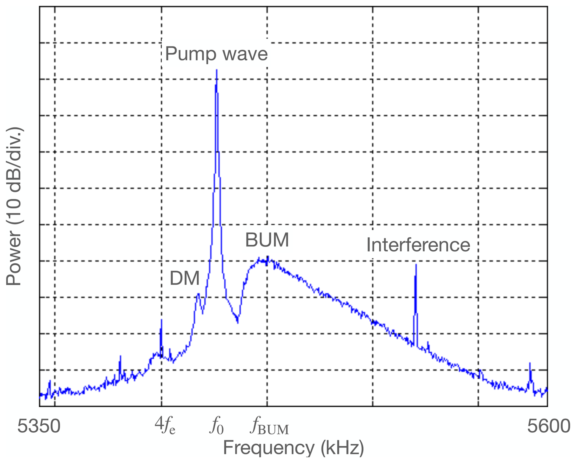
Figure 1 A BUM spectral feature observed in experiments at the SURA HF facility in Russia, with f₀=5.426 MHz, 4f_e≈5.407 MHz, and Δf_BUM≈24 kHz (27 September 1998). Taken from Leyser (2021), where it is adapted from Carozzi et al. (2002).

The frequency of the BUM f_BUM follows the empirical relation (Leyser et al., 1989; Leyser, 2001)

$$\begin{array}{}\text{(3)}& f_{\mathrm{BUM}}-f_{\mathrm{0}}\approx f_{\mathrm{0}}-s{f}_{\mathrm{e}},\end{array}$$

where s≥3. This dependence suggests that the BUM is excited by a parametric four-wave interaction. Huang and Kuo (1994) developed a one-dimensional analytical model involving an electromagnetic pump wave with an angular frequency and wave vector (ω₀, k₀), electron Bernstein (EB) waves (ω₁≲s ω_e, k₁), upper-hybrid (UH) waves (${\mathit{\omega }}_{\mathrm{2}}=\mathrm{2}\mathit{\pi }{f}_{\mathrm{BUM}}\gtrsim s{\mathit{\omega }}_{\mathrm{e}}$, k₂), and non-resonant LH oscillations (ω₃, k₃). The matching conditions in their electrostatic approximation are ${\mathit{\omega }}_{\mathrm{1}}+{\mathit{\omega }}_{\mathrm{3}}={\mathit{\omega }}_{\mathrm{0}}={\mathit{\omega }}_{\mathrm{2}}-{\mathit{\omega }}_{\mathrm{3}}$ and $k_{\mathrm{1}}+k_{\mathrm{3}}=\mathrm{0}=k_{\mathrm{2}}-k_{\mathrm{3}}$. With this, ${\mathit{\omega }}_{\mathrm{3}}\ll {\mathit{\omega }}_{\mathrm{1}}\lesssim {\mathit{\omega }}_{\mathrm{0}}\lesssim {\mathit{\omega }}_{\mathrm{2}}$ (ω_α=2πf_α for $\mathit{\alpha }=\mathrm{0},\mathrm{1},\mathrm{2},\mathrm{3}$). By assuming that the UH mode at ω₂>ω₀ is converted to electromagnetic emissions by the scattering off of filamentary density striations, the emissions could propagate to the ground to be detected as the BUM in the SEE spectrum. The theoretical model was found to be consistent with experimental results and has been verified by numerical simulations of an electrostatic particle-in-cell model with one periodic space dimension and three velocity dimensions (Xi and Scales, 2001).

In the present treatment, a two-fluid model of LH oscillations excited by the beating of an electromagnetic pump field is presented, with EB and UH oscillations assumed to be localized in a cylindrical density depletion in the plane perpendicular to B_g. This complements the study of parametric four-wave interactions by Huang and Kuo (1994) and focuses on the effects of an important nonlinear term for LH dynamics and considers two spatial dimensions. Further, the treatment expands on the study of Leyser (2021) by including the physics of LH oscillations instead of only the associated E×B_g drift. Simulation results are obtained with parameter values that are typical of those in electromagnetic pumping of ionospheric F-region plasma and show deterministic chaos in the LH dynamics and exponential power spectra that are consistent with what is observed for the BUM.

2 Theory

LH dynamics are described by a magnetized electron fluid and an unmagnetized ion fluid. For simplicity, the electron and ion fluids are taken here to be cold; i.e. the electron and ion temperatures are set to zero. All electric fields and velocities are considered to be in the x–y plane perpendicular to a static and homogeneous geomagnetic field ${\mathit{B}}_{\mathrm{g}}=B_{\mathrm{g}}\widehat{\mathit{z}}$.

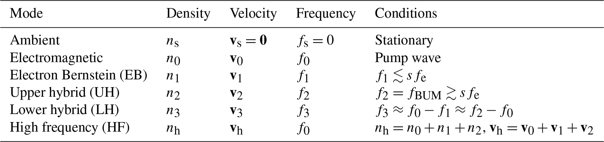
The electron density is taken to be $n_{\mathrm{e}}=n_{\mathrm{s}}+n_{\mathrm{3}}+n_{\mathrm{1}}+n_{\mathrm{2}}\equiv n_{\mathrm{s}}+n_{\mathrm{3}}+n_{\mathrm{h}}$, where n_s is the static background electron density, and n_h contains the HF terms. The electron velocity is ${\mathit{v}}_{\mathrm{e}}={\mathit{v}}_{\mathrm{0}}+{\mathit{v}}_{\mathrm{1}}+{\mathit{v}}_{\mathrm{2}}+{\mathit{v}}_{\mathrm{3}}\equiv {\mathit{v}}_{\mathrm{h}}+{\mathit{v}}_{\mathrm{3}}$, where v_h contains the HF electron velocity terms. For reference, the quantities describing the four interacting wave modes are shown in Table 1. The force and charge continuity equations for v₃ and n₃ at the LH timescale are as follows:

$$\begin{array}{}\text{(4)}& m_{\mathrm{e}}{\displaystyle \frac{\partial {\mathit{v}}_{\mathrm{3}}}{\partial t}}=-e{\mathit{E}}_{\mathrm{3}}-e{\mathit{v}}_{\mathrm{3}}\times {\mathit{B}}_{\mathrm{g}}-m_{\mathrm{e}}\langle ({\mathit{v}}_{\mathrm{h}}\cdot {\mathrm{\nabla }}_{⟂}){\mathit{v}}_{\mathrm{h}}\rangle -{\mathit{\nu }}_{\mathrm{e}}{m}_{\mathrm{e}}{\mathit{v}}_{\mathrm{3}},\end{array}$$

$$\begin{array}{}\text{(5)}& {\displaystyle \frac{\partial n_{\mathrm{3}}}{\partial t}}+{\mathrm{\nabla }}_{⟂}\cdot \left(n_{\mathrm{e}}{\mathit{v}}_{\mathrm{e}}\right)=\mathrm{0},\end{array}$$

where ${\mathrm{\nabla }}_{⟂}\equiv (\partial /\partial x)\widehat{\mathit{x}}+(\partial /\partial y)\widehat{\mathit{y}}$; $\widehat{\mathit{x}}$ and $\widehat{\mathit{y}}$ are unit vectors in the x and y directions, respectively; E₃ is the LH electric field; and ν_e is the electron collision frequency (m_e and −e are the electron mass and charge, respectively). The term $\mathit{F}=m_{\mathrm{e}}\langle ({\mathit{v}}_{\mathrm{h}}\cdot {\mathrm{\nabla }}_{⟂}){\mathit{v}}_{\mathrm{h}}\rangle$ is the ponderomotive force describing the nonlinear low-frequency effect of the HF waves on the electrons, and the angular brackets denote an averaging of the enclosed quantities over the HF oscillations.

Table 1 Parameters for the four wave modes responsible for the broad upshifted maximum (BUM).

With the expressions for n_e and v_e, Eq. (5) gives the following at the LH timescale:

$$\begin{array}{}\text{(6)}& {\displaystyle \frac{\partial n_{\mathrm{3}}}{\partial t}}+(n_{\mathrm{s}}+n_{\mathrm{3}}){\mathrm{\nabla }}_{⟂}\cdot {\mathit{v}}_{\mathrm{3}}+{\mathit{v}}_{\mathrm{3}}\cdot {\mathrm{\nabla }}_{⟂}{n}_{\mathrm{3}}=-{\mathrm{\nabla }}_{⟂}\cdot \langle n_{\mathrm{h}}{\mathit{v}}_{\mathrm{h}}\rangle .\end{array}$$

The last (advection) term on the left-hand side is crucial to include the chaotic dynamics but has commonly been neglected in studies of nonlinear normal mode coupling of parametric interactions. For simplicity, this term is not included self consistently. To investigate the effect of the advection term, v₃ is replaced by an externally provided drift velocity v_D. Equation (6) is further simplified by n_s≫|n₃|, neglecting the effect of static density inhomogeneity (${\mathrm{\nabla }}_{⟂}{n}_{\mathrm{s}}=\mathrm{0}$) and taking ${\mathrm{\nabla }}_{⟂}\cdot \langle n_{\mathrm{h}}{\mathit{v}}_{\mathrm{h}}\rangle \approx \mathrm{0}$ (Istomin and Leyser, 1995), such that

$$\begin{array}{}\text{(7)}& {\displaystyle \frac{\partial n_{\mathrm{3}}}{\partial t}}+n_{\mathrm{s}}{\mathrm{\nabla }}_{⟂}\cdot {\mathit{v}}_{\mathrm{3}}+{\mathit{v}}_{\mathrm{D}}\cdot {\mathrm{\nabla }}_{⟂}{n}_{\mathrm{3}}=\mathrm{0}.\end{array}$$

By noting that the second term on the right-hand side of Eq. (4) is the largest, v₃ can be obtained by iteration (Istomin and Leyser, 1995), giving

$$\begin{array}{ll}{\displaystyle }{\mathit{v}}_{\mathrm{3}}=& {\displaystyle \frac{e}{m_{\mathrm{e}}{\mathit{\omega }}_{\mathrm{e}}}}({\displaystyle \frac{\mathrm{1}}{B_{\mathrm{g}}}}{\mathit{E}}_{\mathrm{3}}\times {\mathit{B}}_{\mathrm{g}}-{\displaystyle \frac{\mathrm{1}}{{\mathit{\omega }}_{\mathrm{e}}}}{\displaystyle \frac{\partial {\mathit{E}}_{\mathrm{3}}}{\partial t}})\\ {\displaystyle }& {\displaystyle }-{\displaystyle \frac{\mathrm{1}}{m_{\mathrm{e}}{\mathit{\omega }}_{\mathrm{e}}}}({\displaystyle \frac{\mathrm{1}}{B_{\mathrm{g}}}}{\mathit{B}}_{\mathrm{g}}\times \mathit{F}+{\displaystyle \frac{\mathrm{1}}{{\mathit{\omega }}_{\mathrm{e}}}}{\displaystyle \frac{\partial \mathit{F}}{\partial t}})\\ \text{(8)}& {\displaystyle }& {\displaystyle }-{\displaystyle \frac{{\mathit{\nu }}_{\mathrm{e}}}{{\mathit{\omega }}_{\mathrm{e}}}}{\displaystyle \frac{\mathrm{1}}{B_{\mathrm{g}}}}{\mathit{E}}_{\mathrm{3}},\end{array}$$

where ${\mathit{\omega }}_{\mathrm{e}}=\mathrm{2}\mathit{\pi }{f}_{\mathrm{e}}=e{B}_{\mathrm{g}}/m_{\mathrm{e}}$, with the last term being included to account for collisional damping. The ponderomotive force is taken to be (Istomin and Leyser, 1995)

$$\begin{array}{}\text{(9)}& \mathit{F}={\displaystyle \frac{\mathrm{1}}{\mathrm{8}}}{\displaystyle \frac{e^{\mathrm{2}}}{m_{\mathrm{e}}}}{\displaystyle \frac{\mathrm{1}}{({\mathit{\omega }}_{\mathrm{0}}+{\mathit{\omega }}_e{)}^{\mathrm{2}}}}{\mathrm{\nabla }}_{⟂}\mathrm{|}{E}_{\mathrm{h}}{\mathrm{|}}^{\mathrm{2}}.\end{array}$$

${\mathit{E}}_{\mathrm{h}}={\mathit{E}}_{\mathrm{0}}+{\mathit{E}}_{\mathrm{1}}+{\mathit{E}}_{\mathrm{2}}$ is the total HF electric field. For simplicity, an additional term that depends on the electron gyro harmonic s derived by Istomin and Leyser (1995) has been neglected.

Substituting Eq. (8) into Eq. (7) to eliminate v₃ gives

$$\begin{array}{}\text{(10)}& {\displaystyle \frac{\partial n_{\mathrm{3}}}{\partial t}}={\displaystyle \frac{e{n}_{\mathrm{s}}}{m_{\mathrm{e}}{\mathit{\omega }}_{\mathrm{e}}^{\mathrm{2}}}}\left({\displaystyle \frac{\partial }{\partial t}}+{\mathit{\nu }}_{\mathrm{e}}\right){\mathrm{\nabla }}_{⟂}\cdot {\mathit{E}}_{\mathrm{3}}+{\displaystyle \frac{n_{\mathrm{s}}}{m_{\mathrm{e}}{\mathit{\omega }}_{\mathrm{e}}^{\mathrm{2}}}}{\displaystyle \frac{\partial }{\partial t}}({\mathrm{\nabla }}_{⟂}\cdot \mathit{F}).\end{array}$$

With the Poisson equation ${\mathit{\epsilon }}_{\mathrm{0}}{\mathrm{\nabla }}_{⟂}\cdot {\mathit{E}}_{\mathrm{3}}=e(n_{\mathrm{i}\mathrm{3}}-n_{\mathrm{3}})$, an equation relating the electron density fluctuations n₃ to those of the ion density n_i3 is obtained as follows (ε₀ is the vacuum permittivity):

$$\begin{array}{}\text{(11)}& \begin{array}{rl}{\displaystyle \frac{\partial n_{\mathrm{3}}}{\partial t}}& ={\displaystyle \frac{{\mathit{\omega }}_{\mathrm{p}}^{\mathrm{2}}}{{\mathit{\omega }}_{\mathrm{uh}}^{\mathrm{2}}}}{\displaystyle \frac{\partial n_{\mathrm{i}\mathrm{3}}}{\partial t}}+{\mathit{\nu }}_{\mathrm{e}}{\displaystyle \frac{{\mathit{\omega }}_{\mathrm{p}}^{\mathrm{2}}}{{\mathit{\omega }}_{\mathrm{uh}}^{\mathrm{2}}}}(n_{\mathrm{i}\mathrm{3}}-n_{\mathrm{3}})-{\displaystyle \frac{{\mathit{\omega }}_{\mathrm{e}}^{\mathrm{2}}}{{\mathit{\omega }}_{\mathrm{uh}}^{\mathrm{2}}}}{\mathit{v}}_{\mathrm{D}}\cdot {\mathrm{\nabla }}_{⟂}{n}_{\mathrm{3}}\\ & +{\displaystyle \frac{n_{\mathrm{s}}}{m_{\mathrm{e}}{\mathit{\omega }}_{\mathrm{uh}}^{\mathrm{2}}}}{\displaystyle \frac{\partial }{\partial t}}({\mathrm{\nabla }}_{⟂}\cdot \mathit{F}),\end{array}\end{array}$$

where ${\mathit{\omega }}_{\mathrm{uh}}^{\mathrm{2}}={\mathit{\omega }}_{\mathrm{p}}^{\mathrm{2}}+{\mathit{\omega }}_{\mathrm{e}}^{\mathrm{2}}$, and ω_p is the electron plasma frequency.

The force and charge continuity equations for the unmagnetized ion fluid are, similarly,

$$\begin{array}{}\text{(12)}& {\displaystyle }{m}_{\mathrm{i}}{\displaystyle \frac{\partial {\mathit{v}}_{\mathrm{i}\mathrm{3}}}{\partial t}}=e{\mathit{E}}_{\mathrm{3}}-{\mathit{\nu }}_{\mathrm{i}}{m}_{\mathrm{i}}{\mathit{v}}_{\mathrm{i}\mathrm{3}},\text{(13)}& {\displaystyle \frac{\partial n_{\mathrm{i}\mathrm{3}}}{\partial t}}+(n_{\mathrm{s}}+n_{\mathrm{i}\mathrm{3}}){\mathrm{\nabla }}_{⟂}\cdot {\mathit{v}}_{\mathrm{i}\mathrm{3}}+{\mathit{v}}_{\mathrm{D}}\cdot {\mathrm{\nabla }}_{⟂}{n}_{\mathrm{i}\mathrm{3}}=\mathrm{0},\end{array}$$

where ν_i is the ion collision frequency. Eliminating v_i3 and using, again, the Poisson equation to eliminate E₃ results in

$$\begin{array}{}\text{(14)}& \begin{array}{rl}\left({\displaystyle \frac{{\partial }^{\mathrm{2}}}{\partial t^{\mathrm{2}}}}+{\mathit{\omega }}_{\mathrm{pi}}^{\mathrm{2}}+{\mathit{\nu }}_{\mathrm{i}}{\displaystyle \frac{\partial }{\partial t}}\right)n_{\mathrm{i}\mathrm{3}}& ={\mathit{\omega }}_{\mathrm{pi}}^{\mathrm{2}}{n}_{\mathrm{3}}-{\displaystyle \frac{\partial {\mathit{v}}_{\mathrm{D}}}{\partial t}}\cdot {\mathrm{\nabla }}_{⟂}{n}_{\mathrm{i}\mathrm{3}}\\ & -{\mathit{v}}_{\mathrm{D}}\cdot {\mathrm{\nabla }}_{⟂}{\displaystyle \frac{\partial n_{\mathrm{i}\mathrm{3}}}{\partial t}}.\end{array}\end{array}$$

Equations (11) and (14) are a coupled set of equations for the electron and ion densities, with n₃ and n_i3 being associated with the LH dynamics driven by the external fields through F and v_D.

In order to relate the electromagnetic pump and EB, UH, and LH fields to one another through F and v_D, it is recalled that the empirical relation in Eq. (3) suggests that the BUM is excited by a parametric four-wave interaction. In two-dimensional cylindrical geometry, the matching conditions are (Karplyuk et al., 1970; Leyser, 2021)

$$\begin{array}{}\text{(15)}& {\displaystyle }{\mathit{\omega }}_{\mathrm{1}}+{\mathit{\omega }}_{\mathrm{3}}={\mathit{\omega }}_{\mathrm{0}}={\mathit{\omega }}_{\mathrm{2}}-{\mathit{\omega }}_{\mathrm{3}},\text{(16)}& {\displaystyle }{m}_{\mathrm{1}}+m_{\mathrm{3}}=m_{\mathrm{0}}=m_{\mathrm{2}}-m_{\mathrm{3}},\end{array}$$

where m_α is the azimuthal mode number (α=0, 1, 2, 3). In cylindrical geometry, there are no matching conditions for the radial wave numbers k_rα.

The ponderomotive force F depends on the HF fields E_h. With the electric fields having the time dependence E_α∝cos (ω_αt), the following terms in relation to F include components that can excite LH oscillations at ω₃ according to the matching condition of Eq. (15):

$$\begin{array}{}\text{(17)}& \mathrm{|}{E}_{\mathrm{h}}{\mathrm{|}}^{\mathrm{2}}={\mathit{E}}_{\mathrm{0}}\cdot {\mathit{E}}_{\mathrm{1}}+{\mathit{E}}_{\mathrm{0}}\cdot {\mathit{E}}_{\mathrm{2}}.\end{array}$$

The pump field is taken to be left-handedly circularly polarized (for which the electric field rotates in opposition to the electron gyro motion):

$$\begin{array}{}\text{(18)}& {\mathit{E}}_{\mathrm{0}}={\displaystyle \frac{E_{\mathrm{0}}}{\sqrt{\mathrm{2}}}}\left[\cos \left({\mathit{\omega }}_{\mathrm{0}}t\right)\widehat{\mathit{x}}-\sin \left({\mathit{\omega }}_{\mathrm{0}}t\right)\widehat{\mathit{y}}\right].\end{array}$$

The EB (α=1) and UH (α=2) oscillations are taken to have the potential

$$\begin{array}{}\text{(19)}& {\mathrm{\Phi }}_{\mathit{\alpha }}=A_{\mathit{\alpha }}{J}_{m_{\mathit{\alpha }}}\left(k_{\mathrm{r}\mathit{\alpha }}\mathit{\rho }\right)\cos (m_{\mathit{\alpha }}\mathit{\phi }+\mathrm{\Delta }{\mathit{\phi }}_{\mathit{\alpha }})\cos \left({\mathit{\omega }}_{\mathit{\alpha }}t\right),\end{array}$$

such that ${\mathit{E}}_{\mathit{\alpha }}=-{\mathrm{\nabla }}_{⟂}{\mathrm{\Phi }}_{\mathit{\alpha }}$, where $J_{m_{\mathit{\alpha }}}$ is the Bessel function of the first kind, $\mathit{\rho }=(x^{\mathrm{2}}+y^{\mathrm{2}}{)}^{\mathrm{1}/\mathrm{2}}$, φ is the azimuthal angle in the x–y plane, and Δφ_α accounts for a possible phase shift between the EB and UH oscillations. With Eqs. (18) and (19) being incorporated into Eq. (17), an expression for F, as in Eq. (9), is obtained.

The largest contribution to v₃ in Eq. (8) is the first term on the right-hand side, which is proportional to E₃×B_g. The drift velocity v_D, which has to be provided, is therefore taken to be ${\mathit{v}}_{\mathrm{D}}={\mathit{E}}_{\mathrm{D}}\times {\mathit{B}}_{\mathrm{g}}/B_{\mathrm{g}}$, where E_D is associated with the beating of the HF fields that give contributions at ω₃. For the present purpose, ${\mathit{E}}_{\mathrm{D}}=-{\mathrm{\nabla }}_{⟂}{\mathrm{\Phi }}_{\mathrm{D}}$:

$$\begin{array}{}\text{(20)}& \begin{array}{rl}{\mathrm{\Phi }}_{\mathrm{D}}& =\left[A_{\mathrm{01}}{J}_{m_{\mathrm{3}}}\right(k_{\mathrm{r}\mathrm{1}}\mathit{\rho }\left)\cos \right(m_{\mathrm{3}}\mathit{\phi })+A_{\mathrm{02}}{J}_{m_{\mathrm{3}}}(k_{\mathrm{r}\mathrm{2}}\mathit{\rho })\\ & \times \cos (m_{\mathrm{3}}\mathit{\phi }+\mathrm{\Delta }{\mathit{\phi }}_{\mathrm{2}})\left]\cos \right({\mathit{\omega }}_{\mathrm{3}}t)e^{-\mathit{\rho }/L},\end{array}\end{array}$$

where A₀₁ (A₀₂) is the potential that results from the beating at ω₃ of the pump field and EB (UH) oscillations and is therefore proportional to the product of E₀ and the amplitude A₁ (A₂) of the EB (UH) oscillations; see Eq. (19). However, it is beyond the scope of the present treatment to derive a relation between them. The focus here is to study the possible influence of the externally provided F and v_D on LH dynamics. The last factor in Eq. (20) is used to model the localization of Φ_D in relation to LH oscillations in a cylindrical density depletion, where L is the decay scale length of the potential outside of the depletion.

3 Simulation scheme

Solutions to Eqs. (11) and (14) are computed numerically. Hereafter, the dimensionless density variables ${\mathit{\eta }}_{\mathrm{3}}\equiv n_{\mathrm{3}}(t,x,y)/n_{\mathrm{s}}$ and ${\mathit{\eta }}_{\mathrm{i}\mathrm{3}}\equiv n_{\mathrm{i}\mathrm{3}}/n_{\mathrm{s}}$ will be used. Further, Eq. (14) is of the second order in the time derivative. In order to solve it numerically, it is converted into two first-order equations by introducing ${\mathit{\eta }}_{\mathrm{i}\mathrm{3}}^{\prime }\equiv n_{\mathrm{i}\mathrm{3}}^{\prime }/n_{\mathrm{s}}$. This gives the following set of three equations:

$$\begin{array}{}\text{(21)}& {\displaystyle }\begin{array}{rl}{\displaystyle \frac{\partial {\mathit{\eta }}_{\mathrm{3}}}{\partial t}}& ={\displaystyle \frac{{\mathit{\omega }}_{\mathrm{p}}^{\mathrm{2}}}{{\mathit{\omega }}_{\mathrm{uh}}^{\mathrm{2}}}}{\mathit{\eta }}_{\mathrm{i}\mathrm{3}}^{\prime }+({\mathit{\eta }}_{\mathrm{i}\mathrm{3}}-{\mathit{\eta }}_{\mathrm{3}}){\mathit{\nu }}_{\mathrm{e}}-{\displaystyle \frac{{\mathit{\omega }}_{\mathrm{e}}^{\mathrm{2}}}{{\mathit{\omega }}_{\mathrm{uh}}^{\mathrm{2}}}}{\mathit{v}}_{\mathrm{D}}\cdot {\mathrm{\nabla }}_{⟂}{\mathit{\eta }}_{\mathrm{3}}\\ & +{\displaystyle \frac{\mathrm{1}}{m_{\mathrm{e}}{\mathit{\omega }}_{\mathrm{uh}}^{\mathrm{2}}}}{\displaystyle \frac{\partial }{\partial t}}({\mathrm{\nabla }}_{⟂}\cdot \mathit{F}),\end{array}\text{(22)}& {\displaystyle \frac{\partial {\mathit{\eta }}_{\mathrm{i}\mathrm{3}}^{\prime }}{\partial t}}={\mathit{\omega }}_{\mathrm{pi}}^{\mathrm{2}}({\mathit{\eta }}_{\mathrm{3}}-{\mathit{\eta }}_{\mathrm{i}\mathrm{3}})-{\mathit{\nu }}_{\mathrm{i}}{\mathit{\eta }}_{\mathrm{i}\mathrm{3}}^{\prime }-{\displaystyle \frac{\partial {\mathit{v}}_{\mathrm{D}}}{\partial t}}\cdot {\mathrm{\nabla }}_{⟂}{\mathit{\eta }}_{\mathrm{i}\mathrm{3}}-{\mathit{v}}_{\mathrm{D}}\cdot {\mathrm{\nabla }}_{⟂}{\mathit{\eta }}_{\mathrm{i}\mathrm{3}}^{\prime },\text{(23)}& {\displaystyle \frac{\partial {\mathit{\eta }}_{\mathrm{i}\mathrm{3}}}{\partial t}}={\mathit{\eta }}_{\mathrm{i}\mathrm{3}}^{\prime }.\end{array}$$

To solve Eqs. (21) to (23) numerically, they are converted into a system of coupled algebraic equations by replacing η₃, η_i3, and ${\mathit{\eta }}_{\mathrm{i}\mathrm{3}}^{\prime }$ with corresponding grid functions that are discretized in time $t=t_j=j\mathrm{\Delta }t$ ($j=\mathrm{0},\mathrm{1},\mathrm{2},$ … ,J) and on an equidistant spatial grid of $x=x_k=k\mathrm{\Delta }d$ and $y=y_l=l\mathrm{\Delta }d$ ($k,l=\mathrm{0},\mathrm{1},\mathrm{2},$ … ,M), such that ${\mathit{\eta }}_{\mathrm{3}}(t_j,x_k,y_l)\approx {\mathit{\eta }}_{\mathrm{3}}^{jkl}$, ${\mathit{\eta }}_{\mathrm{i}\mathrm{3}}(t_j,x_k,y_l)\approx {\mathit{\eta }}_{\mathrm{i}\mathrm{3}}^{jkl}$, and ${\mathit{\eta }}_{\mathrm{i}\mathrm{3}}^{\prime }(t_j,x_k,y_l)\approx {\mathit{\eta }}_{\mathrm{i}\mathrm{3}\prime }^{jkl}$ (Langtangen and Linge, 2017).

The time derivatives of η₃, η_i3, and ${\mathit{\eta }}_{\mathrm{i}\mathrm{3}}^{\prime }$ are approximated with the forward Euler method for the finite differences; for example, $\partial {\mathit{\eta }}_{\mathrm{3}}/\partial t\approx ({\mathit{\eta }}_{\mathrm{3}}^{(j+\mathrm{1})kl}-{\mathit{\eta }}_{\mathrm{3}}^{jkl})/\mathrm{\Delta }t$. All spatial differences are computed at the time step j. Second-order spatial derivatives are approximated by centred differencing; for example, ${\partial }^{\mathrm{2}}{E}_{\mathit{\alpha }x}/\partial x^{\mathrm{2}}\approx (E_{\mathit{\alpha }x}^{j(k+\mathrm{1})l}-\mathrm{2}{E}_{\mathit{\alpha }x}^{jkl}+E_{\mathit{\alpha }x}^{j(k-\mathrm{1})l})/\mathrm{\Delta }{x}^{\mathrm{2}}$. The first-order spatial derivatives of η₃, η_i3, and ${\mathit{\eta }}_{\mathrm{i}\mathrm{3}}^{\prime }$ in the advection terms need a different treatment and are approximated by so-called upwind differencing. For example, in the x direction, with η₃, we take $\partial {\mathit{\eta }}_{\mathrm{3}}/\partial x\approx ({\mathit{\eta }}_{\mathrm{3}}^{jkl}-{\mathit{\eta }}_{\mathrm{3}}^{j(k-\mathrm{1})l})/\mathrm{\Delta }x$ when v_Dx>0 and $\partial {\mathit{\eta }}_{\mathrm{3}}/\partial x\approx ({\mathit{\eta }}_{\mathrm{3}}^{j(k+\mathrm{1})l}-{\mathit{\eta }}_{\mathrm{3}}^{jkl})/\mathrm{\Delta }x$ when v_Dx<0. The direction of the differencing is always against the direction of the drift.

The spatial grid is 4.0×4.0 m, with Δd≈0.025 m. The fields are localized around the centre of the grid $(x,y)=(\mathrm{0},\mathrm{0})$ m by multiplication of a factor $\exp (-\mathit{\rho }/L)$ with L=0.4 m. All parameters are zero at the boundaries: ${\mathit{\eta }}_{\mathrm{3}}^{j\mathrm{0}l}={\mathit{\eta }}_{\mathrm{3}}^{jMl}=\mathrm{0}$ and ${\mathit{\eta }}_{\mathrm{3}}^{jk\mathrm{0}}={\mathit{\eta }}_{\mathrm{3}}^{jkM}=\mathrm{0}$, ${\mathit{\eta }}_{\mathrm{i}\mathrm{3}}^{j\mathrm{0}l}={\mathit{\eta }}_{\mathrm{i}\mathrm{3}}^{jMl}=\mathrm{0}$ and ${\mathit{\eta }}_{\mathrm{i}\mathrm{3}}^{jk\mathrm{0}}={\mathit{\eta }}_{\mathrm{i}\mathrm{3}}^{jkM}=\mathrm{0}$, and ${\mathit{\eta }}_{\mathrm{i}\mathrm{3}\prime }^{j\mathrm{0}l}={\mathit{\eta }}_{\mathrm{i}\mathrm{3}\prime }^{jMl}=\mathrm{0}$ and ${\mathit{\eta }}_{\mathrm{i}\mathrm{3}\prime }^{jk\mathrm{0}}={\mathit{\eta }}_{\mathrm{i}\mathrm{3}\prime }^{jkM}=\mathrm{0}$.

The time step is $\mathrm{\Delta }t=\mathrm{2.5}\times {\mathrm{10}}^{-\mathrm{7}}$ s. The initial conditions of the spatial grid are taken such that ${\mathit{\eta }}_{\mathrm{3}}^{\mathrm{0}kl}\propto {\mathrm{\Phi }}_{\mathrm{D}}(t=\mathrm{0})$ in Eq. (20):

$$\begin{array}{}\text{(24)}& \begin{array}{rl}{\mathit{\eta }}_{\mathrm{3}}^{\mathrm{0}kl}& ={\displaystyle \frac{N_{\mathrm{3}}}{(A_{\mathrm{01}}^{\mathrm{2}}+A_{\mathrm{02}}^{\mathrm{2}}{)}^{\mathrm{1}/\mathrm{2}}}}\left(A_{\mathrm{01}}{J}_{m_{\mathrm{1}}}\left(k_{\mathrm{r}\mathrm{1}}{\mathit{\rho }}_{kl}\right)\cos \left(m_{\mathrm{1}}{\mathit{\phi }}_{kl}\right)\right.\\ & \left.+A_{\mathrm{02}}{J}_{m_{\mathrm{2}}}\left(k_{\mathrm{r}\mathrm{2}}{\mathit{\rho }}_{kl}\right)\cos (m_{\mathrm{2}}{\mathit{\phi }}_{kl}+\mathrm{\Delta }{\mathit{\phi }}_{\mathrm{2}})\right)e^{-\mathit{\rho }/L},\end{array}\end{array}$$

where A₀₁ and A₀₂ allow for different relative amplitudes of the EB and UH potentials. Further, ${\mathit{\eta }}_{\mathrm{i}\mathrm{3}}^{\mathrm{0}kl}=({\mathit{\omega }}_{\mathrm{uh}}^{\mathrm{2}}/{\mathit{\omega }}_{\mathrm{p}}^{\mathrm{2}}){\mathit{\eta }}_{\mathrm{3}}^{\mathrm{0}kl}$, and ${\mathit{\eta }}_{\mathrm{i}\mathrm{3}\prime }^{\mathrm{0}kl}=\mathrm{0}$.

4 Simulation results

As an example, the azimuthal mode numbers of the interacting wave modes are taken to be m₀=1, $m_{\mathrm{1}}=-\mathrm{1}$, and m₂=3, which, using Eq. (16), gives m₃=2. In the experiments, the transmitted electromagnetic pump wave is approximately a left-handed circularly polarized plane wave on the small-spatial-scale lengths of interest here, propagating nearly parallel to B_g. However, its scattering on filamentary density depletions with much-smaller-spatial-scale lengths transverse to B_g compared to the electromagnetic wavelength can give an azimuthal component of the pump field (Istomin and Leyser, 2003). This is the motivation for why m₀=1 is taken here, which implies that m₁≠m₂ for m₃≠0. Figure 2 shows the initial ${\mathit{\eta }}_{\mathrm{3}}^{\mathrm{0}kl}$, as given by Eq. (24), in the centre of the simulation plane perpendicular to B_g. The magnitude of $N_{\mathrm{3}}=\mathrm{1.0}\times {\mathrm{10}}^{-\mathrm{7}}$ is chosen, such that F in the right-hand side of Eq. (21) has an effect on the temporal evolution, with reasonable values for the external amplitudes E₀, A₁, A₂ A₀₁, and A₀₂.

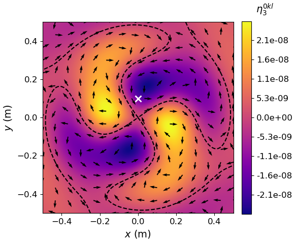
Figure 2 Initial relative electron density distribution ${\mathit{\eta }}_{\mathrm{3}}^{\mathrm{0}kl}$ for the LH oscillations in the centre of the 4×4 m simulation plane according to Eq. (24) ($N_{\mathrm{3}}=\mathrm{1.0}\times {\mathrm{10}}^{-\mathrm{7}}$, $A_{\mathrm{01}}=A_{\mathrm{02}}=\mathrm{0.2}$ V, $\mathrm{\Delta }{\mathit{\phi }}_{\mathrm{2}}=\mathit{\pi }/\mathrm{2}$). The arrows indicate the direction of the E_D×B_g drift. The dashed lines delineate ${\mathit{\eta }}_{\mathrm{3}}^{\mathrm{0}kl}=\mathrm{0}$, constituting separatrices for the drift. The white cross at $(x,y)=(\mathrm{0.0},\mathrm{0.1})$ m marks the position where the time signal and power spectrum are shown in the subsequent figures. The position is relatively near an initial separatrix of the drift.

Figure 3 displays the computed electron and ion densities – ${\mathit{\eta }}_{\mathrm{3}}^{jkl}$ (blue) and ${\mathit{\eta }}_{\mathrm{i}\mathrm{3}}^{jkl}$ (red), respectively – at $(x,y)=(\mathrm{0.0},\mathrm{0.1})$ m for (a) E₀=0.001 V m⁻¹ and $A_{\mathrm{01}}=A_{\mathrm{02}}=\mathrm{0.002}$ V and (b) E₀=0.1 V m⁻¹ and $A_{\mathrm{01}}=A_{\mathrm{02}}=\mathrm{0.2}$ V, with $A_{\mathrm{1}}=A_{\mathrm{2}}=\mathrm{0.2}$ V in both cases. Parameters typical of the ionospheric F region were used: ${\mathit{\omega }}_{\mathrm{e}}\approx \mathrm{2}\mathit{\pi }\times \mathrm{1.35}\times {\mathrm{10}}^{\mathrm{6}}$ s⁻¹, as estimated from the experiments (Carozzi et al., 2002) from which the spectrum in Fig. 1 was obtained, oxygen ions; ω_uh=s ω_e, with s=4, ν_e=500 s⁻¹, and ν_i=5 s⁻¹; and electron temperature T_e=2000 K. The frequencies of the involved wave modes are related by the matching condition of Eq. (15), where, for the present treatment, ${\mathit{\omega }}_{\mathrm{1}}=\mathrm{4}{\mathit{\omega }}_{\mathrm{e}}-\mathrm{\Delta }{\mathit{\omega }}_{\mathrm{1}}$, where $\mathrm{\Delta }{\mathit{\omega }}_{\mathrm{1}}=\mathrm{2}\mathit{\pi }\times \mathrm{10}\times {\mathrm{10}}^{\mathrm{3}}$ s⁻¹. By keeping ω₁ constant, k_r1 is constant, while, for the small value of Δω₁, we still have ω₀≈4 ω_e for the different ω₃ values to be discussed. In the experiments, ω₀≈4 ω_e commonly results in the exponential slope of the BUM spectral feature that is of interest here.

In Fig. 3a, the external driving due to E₀ is weak, such that v_D and F in Eqs. (21) and (22) are small. The displayed oscillations are the LH resonance oscillations at about 7.6 kHz that are weakly perturbed by the beating of the HF fields at f₃=20 kHz in v_D and F. For comparison, a sinusoidal oscillation at f₃ is shown in black. The oscillation frequency in Fig. 3a agrees with the theoretical value of the LH resonance frequency:

$$\begin{array}{}\text{(25)}& f_{\mathrm{lh}}={\displaystyle \frac{\mathrm{1}}{\mathrm{2}\mathit{\pi }}}{\displaystyle \frac{{\mathit{\omega }}_{\mathrm{pi}}{\mathit{\omega }}_{\mathrm{e}}}{{\mathit{\omega }}_{\mathrm{uh}}}}=\left({\displaystyle \frac{m_{\mathrm{e}}}{m_{\mathrm{i}}}}{)}^{\mathrm{1}/\mathrm{2}}\right(\mathrm{1}-{\displaystyle \frac{\mathrm{1}}{s^{\mathrm{2}}}}{)}^{\mathrm{1}/\mathrm{2}}{f}_{\mathrm{e}}\approx \mathrm{7.6}\mathrm{kHz},\end{array}$$

where ${\mathit{\omega }}_{\mathrm{pi}}=(m_{\mathrm{e}}/m_{\mathrm{i}}{)}^{\mathrm{1}/\mathrm{2}}{\mathit{\omega }}_{\mathrm{p}}$. The time step in the computations – $\mathrm{\Delta }t=\mathrm{2.5}\times {\mathrm{10}}^{-\mathrm{7}}$ s – implies $\mathrm{\Delta }t{f}_{\mathrm{lh}}\approx \mathrm{1.9}\times {\mathrm{10}}^{-\mathrm{3}}$. In Fig. 3b, E₀ is sufficiently strong, such that the temporal evolution is instead determined by v_D and F. The temporal evolution contains narrow pulses that are even shorter than the oscillations at the driving frequency f₃ illustrated in Fig. 3a.

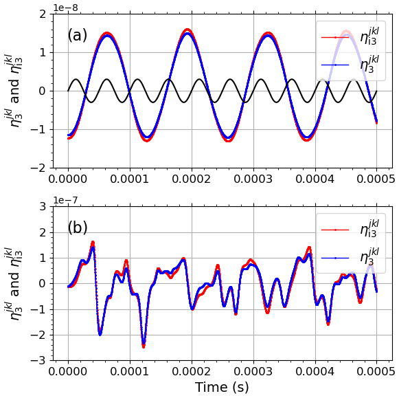
Figure 3 Temporal evolution of ${\mathit{\eta }}_{\mathrm{3}}^{jkl}$ and ${\mathit{\eta }}_{\mathrm{i}\mathrm{3}}^{jkl}$ at k and l, such that $(x,y)=(\mathrm{0.0},\mathrm{0.1})$ m from 0 to 0.0005 s (f₃=20 kHz, $\mathrm{\Delta }{\mathit{\phi }}_{\mathrm{2}}=\mathit{\pi }/\mathrm{2}$). (a) E₀=0.001 V m⁻¹, $A_{\mathrm{1}}=A_{\mathrm{2}}=\mathrm{0.2}$ V, and $A_{\mathrm{01}}=A_{\mathrm{02}}=\mathrm{0.002}$ V. For comparison, shown in black is an oscillation sin (ω₃t) at the driving frequency f₃. (b) E₀=0.1 V m⁻¹, $A_{\mathrm{01}}=A_{\mathrm{02}}=\mathrm{0.2}$ V, and other parameter values as for (a).

Figure 4 displays the temporal evolution (panel a) of ${\mathit{\eta }}_{\mathrm{3}}^{jkl}$ (blue) and ${\mathit{\eta }}_{\mathrm{i}\mathrm{3}}^{jkl}$ (red) and the corresponding power spectrum (panel b) for the longer time period from t=0 s to t=0.0025 s, with the same parameter values as for Fig. 3b. The power spectrum is approximately exponential as it has a constant slope in the semi-logarithmic plot. The narrow peaks at multiples of f₃=20 kHz enter through v_D and F in Eqs. (21) and (22). The width of the LH spectrum is about 160 kHz, which is an order of magnitude larger than both f_lh and f₃.

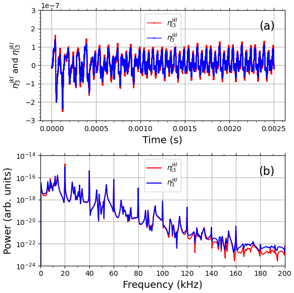
Figure 4 Temporal evolution (a) and power spectrum (b) of ${\mathit{\eta }}_{\mathrm{3}}^{jkl}$ (blue) and ${\mathit{\eta }}_{\mathrm{i}\mathrm{3}}^{jkl}$ (red) at $(x,y)=(\mathrm{0.0},\mathrm{0.1})$ m for the time between 0 s and 0.0025 s, with the same parameter values as for Fig. 3b.

In Figs. 5 and 6, some of the narrow pulses in the temporal evolution of ${\mathit{\eta }}_{\mathrm{3}}^{jkl}$ in Fig. 4a are investigated. Figure 5a shows ${\mathit{\eta }}_{\mathrm{3}}^{jkl}$ from t=0.0005 s to t=0.0025 s, which corresponds to a timescale of $\mathrm{0.0005}\times f_{\mathrm{lh}}\approx \mathrm{4}$ to $\mathrm{0.0025}\times f_{\mathrm{lh}}\approx \mathrm{19}$ wave periods of LH resonance oscillations. The time period excludes the initial overshoot behaviour of ${\mathit{\eta }}_{\mathrm{3}}^{jkl}$ seen in Fig. 4a. The four pairs of vertical dashed red lines mark the time periods with pulse-type features discussed in Fig. 5b and c (t≈0.00067 s) and Fig. 6 (t≈0.00092, 0.00182, and 0.00214 s). Figure 5b displays an expanded time period marked by the vertical dashed red lines at t≈0.00067 s, which includes a single negative pulse-type feature in the time series (blue dots) together with a fitted Lorentzian function in accordance with Eq. (1) (black curve). The width of the Lorentzian pulse is $\mathit{\tau }\approx \mathrm{8.90}\times {\mathrm{10}}^{-\mathrm{6}}$ s, such that τf₃≈0.18, which implies that the temporal pulse is much shorter than the driving wave period ($\mathrm{1}/f_{\mathrm{3}}$). The corresponding scaling frequency is $f_{\mathrm{s}}=\mathrm{1}/\left(\mathrm{4}\mathit{\pi }\mathit{\tau }\right)\approx \mathrm{9}$ kHz. Figure 5c shows the power spectrum (blue) of the time series in Fig. 5a, together with $P\left(f\right)\propto \exp (-f/f_{\mathrm{s}})$ (dashed black line). The width τ and corresponding scaling frequency f_s of the approximately Lorentzian-shaped pulse in Fig. 5b correspond roughly to the slope of the spectrum.

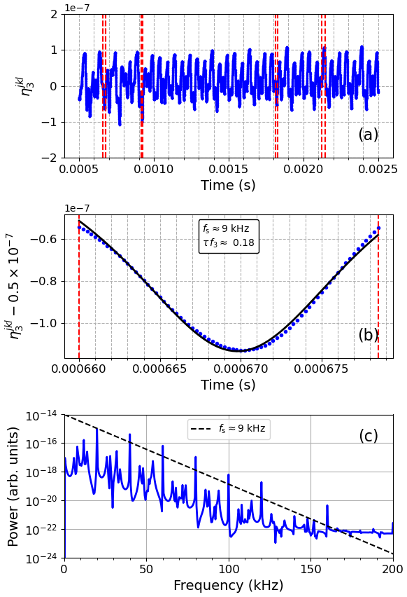
Figure 5 Fit of a Lorentzian function to a single pulse-type feature in the signal of ${\mathit{\eta }}_{\mathrm{3}}^{jkl}$ for the same time series as in Fig. 4 (f₃=20 kHz and E₀=0.1 V m⁻¹). (a) Temporal evolution from t=0.0005 s to t=0.0025 s and (b) for a single pulse (blue dots). The time period for the single pulse is marked by the leftmost pair of vertical dashed red lines at t≈0.0067 s in (a). The three remaining pairs of vertical dashed lines indicate the time periods discussed in Fig. 6. The solid black curve in (b) is a fitted Lorentzian pulse of width $\mathit{\tau }\approx \mathrm{8.90}\times {\mathrm{10}}^{-\mathrm{6}}$ s, which corresponds to f_s≈9 kHz. (c) The power spectrum for the time series in (a). The dashed line shows the exponential slope $P={\mathrm{10}}^{-\mathrm{6}}\exp (-f/f_{\mathrm{s}})$.

Figure 6 displays three additional pulse-type features in the same time series of ${\mathit{\eta }}_{\mathrm{3}}^{jkl}$ (Figs. 4 and 5a) from the time periods at (a) t≈0.00092 s, (b) t≈0.00182 s, and (c) t≈0.00214 s, marked by the three rightmost pairs of dashed red vertical lines in Fig. 5a. In Fig. 6a, the fitted Lorentzian pulse has a width of $\mathit{\tau }\approx \mathrm{6.15}\times {\mathrm{10}}^{-\mathrm{6}}$ s and f_s≈13 kHz. In Fig. 6b, the fitted Lorentzian pulse is $\mathit{\tau }\approx \mathrm{7.23}\times {\mathrm{10}}^{-\mathrm{6}}$ s and f_s≈11 kHz. Most of the pulse-type features in the time series in Fig. 5a have a skewed shape, and only a few have a reasonably symmetric Lorentzian form. Figure 6c shows an example of a skewed pulse. A Lorentzian function cannot be reasonably fitted to the pulse. In Fig. 6d, the same spectrum as in Fig. 5c is displayed but with the spectral slopes for the obtained f_s of the Lorentzian functions: (a) f_s≈13 kHz (dotted line) and (b) f_s≈11 kHz (dash-dotted line). The Lorentzian pulse widths are consistent with the slope of the spectrum. As different widths of Lorentzian pulses give different f_s values, an observed exponential slope is associated with a temporal evolution containing predominantly Lorentzian pulses of approximately equal width, as for Fig. 5b (f_s≈9 kHz), Fig. 6a (f_s≈13 kHz), and Fig. 6b (f_s≈11 kHz).

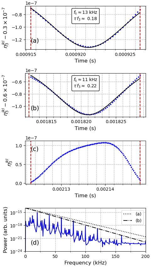
Figure 6 Three examples of pulse-type features from the computed time series ${\mathit{\eta }}_{\mathrm{3}}^{jkl}$ (blue dots) in Figs. 4 and 5a and fits of a Lorentzian function (black lines). (a) Pulse at t≈0.00092 s and fitted Lorentzian function with f_s≈13 kHz (${\mathit{\eta }}_{\mathrm{3}}^{jkl}$ was decreased by $\mathrm{0.3}\times {\mathrm{10}}^{-\mathrm{7}}$ to optimize the fit). (b) Pulse at t≈0.00182 s and f_s≈11 kHz (${\mathit{\eta }}_{\mathrm{3}}^{jkl}$ was decreased by $\mathrm{0.6}\times {\mathrm{10}}^{-\mathrm{7}}$ to optimize the fit). (c) Pulse at t≈0.00214 s. (d) The power spectrum (the same as in Fig. 5c), with the black lines showing the exponential slope $P={\mathrm{10}}^{-\mathrm{14}}\exp (-f/f_{\mathrm{s}})$ for the pulses in (a) and (b).

The width τ of the approximately Lorentzian-shaped pulses in the time series ${\mathit{\eta }}_{\mathrm{3}}^{jkl}$ at a given (x,y) depends on the amplitudes E₀, A₁, A₂, A₀₁, and A₀₂. Figure 7 displays a case with E₀=0.2 V m⁻¹, $A_{\mathrm{01}}=A_{\mathrm{02}}=\mathrm{0.4}$ V, and other parameters, as for Figs. 4 to 6, for which E₀=0.1 V m⁻¹ and $A_{\mathrm{01}}=A_{\mathrm{02}}=\mathrm{0.2}$ V. Figure 7a shows the time series at $(x,y)=(\mathrm{0.0},\mathrm{0.1})$ m. The two pairs of dashed red lines at t≈0.00057 s and t≈0.00077 s indicate two examples of negative pulse-type signatures that have approximately Lorentzian shapes. In Fig. 7b, the pulse (blue dots) at t≈0.00057 s is displayed together with a fitted Lorentzian function (black line) with a width corresponding to f_s≈13 kHz. In Fig. 7c, the pulse (blue dots) at t≈0.00077 s is shown with a fitted Lorentzian function (black line) with a width corresponding to f_s≈15 kHz. The associated exponential slopes agree approximately with that of the power spectrum of the time series seen in Fig. 7d. The pulse in Fig. 7c with f_s≈15 kHz appears to have a slightly better fit to the spectrum. The obtained scaling frequencies of f_s≈13 kHz and f_s≈15 kHz are a few kilohertz higher than those in Figs. 5 and 6, for which f_s≈9, 11, and 13 kHz. Stronger driving through E₀, A₀₁, and A₀₂ gives a larger drift – ${\mathit{v}}_{\mathrm{D}}={\mathit{E}}_{\mathrm{D}}\times {\mathit{B}}_{\mathrm{g}}/B_{\mathrm{g}}$ – and, thereby, narrower pulses with larger f_s.

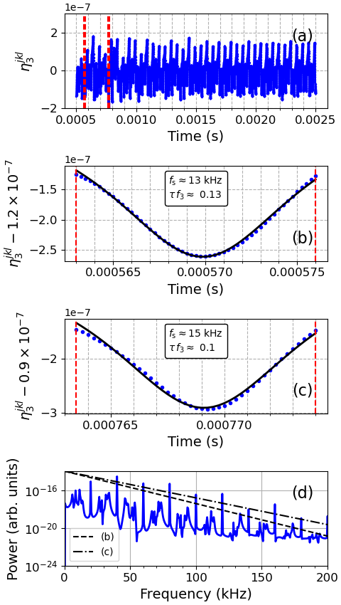
Figure 7 Lorentzian pulse-type features in the computed time signal of ${\mathit{\eta }}_{\mathrm{3}}^{jkl}$ at $(x,y)=(\mathrm{0.0},\mathrm{0.1})$ m for E₀=0.2 V m⁻¹, $A_{\mathrm{01}}=A_{\mathrm{02}}=\mathrm{0.4}$ V, and other parameter values, as for Figs. 4 to 6. (a) Temporal evolution from t=0.0005 s to t=0.0025 s. Two pulses are indicated by the two pairs of vertical red dashed lines. (b) Pulse (blue dots) at t≈0.00057 s and fitted Lorentzian function (solid black curve) of width $\mathit{\tau }\approx \mathrm{6.27}\times {\mathrm{10}}^{-\mathrm{6}}$ s, which corresponds to f_s≈13 kHz (${\mathit{\eta }}_{\mathrm{3}}^{jkl}$ was decreased by $\mathrm{1.2}\times {\mathrm{10}}^{-\mathrm{7}}$ to optimize the fit). (c) Pulse (blue dots) at t≈0.00077 s and fitted Lorentzian function (solid black curve) of width $\mathit{\tau }\approx \mathrm{5.25}\times {\mathrm{10}}^{-\mathrm{6}}$ s, which corresponds to f_s≈15 kHz (${\mathit{\eta }}_{\mathrm{3}}^{jkl}$ was decreased by $\mathrm{0.9}\times {\mathrm{10}}^{-\mathrm{7}}$ to optimize the fit). (d) The power spectrum for the time series in (a). The black lines show the exponential slope $P={\mathrm{10}}^{-\mathrm{14}}\exp (-f/f_{\mathrm{s}})$ for f_s in (b) and (c).

5 Discussion

Plasma drifts in multi-cell patterns may exhibit deterministic chaos due to topological modulations of the flow (e.g. Shi et al., 2009; Maggs and Morales, 2011, 2012). The topological modulations result in the formation of narrow temporal pulses of Lorentzian shape in the plasma flow. As the power spectrum of a Lorentzian pulse is exponential, it follows that, if the Lorentzian pulses in the time signal have approximately the same widths, its spectrum will be exponential. Exponential power spectra are an inherent characteristic of deterministic chaos.

The BUM feature in the spectrum of electromagnetic emissions stimulated by powerful radio waves in the ionosphere commonly exhibits an exponential high-frequency flank, as shown in Fig. 1. The BUM has been attributed to parametric four-wave interactions involving the electromagnetic pump wave and electrostatic EB, UH, and LH waves (Huang and Kuo, 1994), with matching conditions for the high-frequency waves, as suggested by the empirical relation in Eq. (3). In the theory, the UH oscillations at ${\mathit{\omega }}_{\mathrm{2}}={\mathit{\omega }}_{\mathrm{0}}+{\mathit{\omega }}_{\mathrm{3}}$ are assumed to scatter off small-scale density irregularities into electromagnetic emissions that can escape the ionosphere and be detected as the BUM on the ground. Whereas the initial theory by Huang and Kuo (1994) considered waves in one spatial dimension, the present understanding is that, on thermal timescales, wave modes perpendicular to B_g are localized inside density depletions of small-scale striations (Gurevich et al., 1997; Mjølhus, 1997; Istomin and Leyser, 1998). In two-dimensional geometry perpendicular to B_g, excited localized wave modes will have standing multi-cell oscillations inside the density depletions.

In the present treatment, results of numerical simulations of relevant nonlinear wave processes are presented. LH oscillations are modelled by Eqs. (11) and (14) in the plane perpendicular to B_g and are excited by nonlinear interactions of the pump and EB and UH modes. Specifically, the beating of the pump field with the EB and UH fields is introduced through the ponderomotive force F and the drift velocity v_D in the advection terms in the equations. Figure 2 shows the initial condition for the electron density fluctuations ${\mathit{\eta }}_{\mathrm{3}}^{\mathrm{0}kl}$. With ${\mathit{\eta }}_{\mathrm{3}}^{\mathrm{0}kl}\propto {\mathrm{\Phi }}_{\mathrm{D}}(t=\mathrm{0})$, the E_D×B_g drift occurs along equipotential lines around extrema in ${\mathit{\eta }}_{\mathrm{3}}^{jkl}$. Thus, the direction of the E_D×B_g drift changes from clockwise to anti-clockwise and vice versa in adjacent extrema in Φ_D and ${\mathit{\eta }}_{\mathrm{3}}^{jkl}$. The resulting separatrices in the E_D×B_g drift are illustrated by dashed lines in Fig. 2. Also, the drift changes direction with the change in sign of E_D every half wave period $T_{\mathrm{3}}/\mathrm{2}=\mathrm{1}/\left(\mathrm{2}{f}_{\mathrm{3}}\right)$.

Figure 3 displays the temporal evolution of the LH electron ${\mathit{\eta }}_{\mathrm{3}}^{jkl}$ (blue) and ion ${\mathit{\eta }}_{\mathrm{i}\mathrm{3}}^{jkl}$ (red) density fluctuations at $(x,y)=(\mathrm{0.0},\mathrm{0.1})$ m for (a) E₀=0.001 V m⁻¹ and $A_{\mathrm{01}}=A_{\mathrm{02}}=\mathrm{0.002}$ V and (b) E₀=0.1 V m⁻¹ and $A_{\mathrm{01}}=A_{\mathrm{02}}=\mathrm{0.2}$ V, with f₃=20 kHz and $A_{\mathrm{1}}=A_{\mathrm{2}}=\mathrm{0.2}$ V in both cases. In Fig. 3a, ${\mathit{\eta }}_{\mathrm{3}}^{jkl}$ and ${\mathit{\eta }}_{\mathrm{i}\mathrm{3}}^{jkl}$ oscillate at the LH resonance frequency of 7.6 kHz, which is lower than at f₃. Because of the low E₀, the external driving through F and v_D at f₃ is too weak to have a noticeable effect on the time dependence. However, in Fig. 3b, the temporal evolution is different, with pulse-type features occurring seemingly erratically, some of which are narrower than the driving frequency at f₃, indicated by the black curve in Fig. 3a.

Figure 4a shows the electron ${\mathit{\eta }}_{\mathrm{3}}^{jkl}$ (blue) and ion ${\mathit{\eta }}_{\mathrm{i}\mathrm{3}}^{jkl}$ (red) oscillations for the same parameter values as in Fig. 3b but for the longer time period between 0 s and 0.0025 s. As seen in Fig. 4b, the power spectra of both ${\mathit{\eta }}_{\mathrm{3}}^{jkl}$ and ${\mathit{\eta }}_{\mathrm{i}\mathrm{3}}^{jkl}$ have an approximately exponential slope. Figures 5 and 6, which are for the same time period, show that some of the pulse-type features in the time series have close to a Lorentzian shape. The examples in Figs. 5 and 6 give, for the fitted Lorentzian functions, the scaling frequencies f_s≈9 kHz (Fig. 5b), f_s≈13 kHz (Fig. 6b), and f_s≈11 kHz (Fig. 6c). As the obtained f_s values agree approximately with the slope of the spectrum, it is concluded that the power spectra in Figs. 4b, 5b, and 6d are determined by Lorentzian pulses due to chaotic dynamics and that the Lorentzian pulses have approximately the same widths. In the discussed model, with the frequency matching conditions in Eq. (15), the spectrum of LH oscillations (ω₃) is upshifted to the UH mode according to ${\mathit{\omega }}_{\mathrm{2}}={\mathit{\omega }}_{\mathrm{0}}+{\mathit{\omega }}_{\mathrm{3}}$. The UH oscillations could then scatter off density irregularities of the filamentary density striations into electromagnetic emissions that can be detected as the BUM in the SEE spectrum on the ground. It is therefore concluded that the experimentally observed exponential high-frequency flank of the BUM emission (Fig. 1) is evidence of deterministic chaos in wave interactions along the lines of those shown in the present simulations.

The temporal evolution is chaotic for E₀=0.1 V m⁻¹ (Figs. 3b, 4, 5, and 6) but not for E₀=0.001 V m⁻¹ (Fig. 3a). This is evidence that a threshold must be exceeded for chaotic time dependence. Because of temporal modulations in the multi-cell drift trajectories associated with Φ_D, plasma may cross separatrices in the E_D×B_g drift. Deterministic chaos seems to set in when the drift is fast enough for plasma to drift sufficiently far to cross a separatrix to drift around an adjacent potential extremum before the potential changes sign every half wave period and the drift direction reverses.

Whereas some of the pulse-type features in the time series have an approximately Lorentzian form, most of them are asymmetric, and the later pulse flank is generally steeper than the earlier flank. This asymmetry may indicate nonlinear steepening of the pulses. A careful look reveals that this is also the case for the reasonably symmetric Lorentzian pulses in Figs. 5 to 7. It is interesting that the skewness of a Lorentzian pulse does not affect its power spectrum (Maggs and Morales, 2011; Garcia and Theodorsen, 2018), such that asymmetric Lorentzian pulses contribute to an exponential power spectrum. However, it is not clear whether some of the skewed pulses observed in the present simulations can actually be considered to be skewed Lorentzian forms. This requires further investigation.

Finally, the scaling frequency f_s in the present model depends on E₀, A₀₁, and A₀₂. Figure 7 shows a case for E₀=0.2 V m⁻¹, $A_{\mathrm{01}}=A_{\mathrm{02}}=\mathrm{0.4}$ V, and other parameter values, as for Figs. 4 to 6. The obtained f_s values for the fitted Lorentzian functions are typically a few kilohertz higher than for E₀=0.1 V m⁻¹ and $A_{\mathrm{01}}=A_{\mathrm{02}}=\mathrm{0.2}$ V (Figs. 5 and 6). With increasing E₀, f_s increases. However, experiments on pump power stepping at the SURA facility suggest that the slope of the BUM high-frequency flank is independent of the pump power (Wagner et al., 1999, their Fig. 9). The maximum effective radiated power (ERP) was about 150 MW, and the BUM flank was observed to have similar slopes for the pump power levels of −6, −3, and 0 dB relative to the maximum ERP.

The present simulation results are not consistent with this experimental result. As seen from Fig. 7, for which f_s values for the fitted Lorentzian functions in Fig. 7b and c are a few kilohertz larger than in Figs. 5 and 6, f_s depends on E₀, A₀₁, and A₀₂. At this stage, possible reasons for this discrepancy may only be speculated upon. In the present study, only a single density depletion associated with a single small-scale striation is considered. In reality, many striations are excited simultaneously. Theories (Mjølhus, 1983; Gurevich et al., 1995; Hall and Leyser, 2003) and numerical computations (Eliasson and Leyser, 2015) show that striations are electromagnetically coupled to one another through the electromagnetic Z mode. It is brought into question whether, for sufficiently high pump powers, the nonlinear processes of oscillations localized inside a striation are nonlinearly saturated. Increasing the pump power may then only result in more striations to be excited. This could account for the higher BUM intensity at higher pump power but with f_sl that depends on the localized interactions independent of pump power. However, this requires modelling of the physics on a global scale, with many striations and with nonlinear saturation for the involved oscillation amplitudes, which is beyond the scope of the present study.

6 Conclusions

The prominent BUM feature in the spectrum of electromagnetic emissions stimulated by powerful HF radio waves in the ionosphere commonly has an exponential high-frequency flank for pump frequencies near a harmonic of the ionospheric electron gyro frequency. Exponential power spectra have been shown to be a characteristic of deterministic chaos. As the BUM has been interpreted in terms of parametric four-wave interactions involving the electromagnetic pump field and EB, UH, and non-resonant LH modes (Huang and Kuo, 1994), a simplified two-fluid model of parametrically excited LH oscillations has been derived and studied by means of numerical simulations. The LH oscillations were taken to be localized in a cylindrical density depletion in the plane perpendicular to a homogeneous and static geomagnetic field. As such, they form cylindrical modes characterized by the frequency, an azimuthal mode number and radial wave number. The localized LH modes are associated with multi-cell plasma drift patterns. For sufficiently strong driving fields, the time signal of the LH electron and ion density fluctuations at a fixed position in the simulation plane exhibit an approximately exponential power spectrum, thereby being evidence of deterministic chaos. The exponential spectrum is connected to pulse-type features of Lorentzian form in the time signal.

As the parameter values in the simulations are reasonable within the ionospheric experiments, it is proposed that the observed exponential flank of the BUM is the result of deterministic chaos in the LH dynamics. According to the model of parametric interaction for the BUM, the beating of the LH oscillations with the pump field shifts the LH spectrum to the UH mode at frequencies above the pump frequency, where they could be converted into electromagnetic emissions and be observed on the ground. In view of the generality of the physics of deterministic chaos, it may be that similar processes can occur in other regions of space plasma, for example, in ionospheric single- or multi-cell convection that is topologically modulated by fluctuations in the geomagnetic field.