Quadratic magnetic gradients from seven- and nine-spacecraft constellations

To uncover the dynamics of magnetized plasma, it is crucial to determine the geometric structure of the magnetic field, which depends on its linear and quadratic spatial gradients. Estimating the linear magnetic gradient requires at least 4 simultaneous magnetic measurements, while calculating the quadratic gradients generally requires at least 10. This study focuses on deriving both linear and quadratic spatial gradients of the magnetic field using data from the nine-spacecraft (9S/C) HelioSwarm or seven-spacecraft (7S/C) Plasma Observatory constellations. Time series magnetic measurements, combined with transformations between reference frames, were employed to determine the apparent velocity of the magnetic structure and the quadratic magnetic gradient components along the direction of motion. The linear gradient and remaining components of the quadratic gradient were derived using the least-squares method with iterative calculations applied to ensure precision. The validity of the approach was demonstrated using magnetic flux ropes and dipole magnetic field models. The findings indicate that constellations with at least seven spacecraft in nonplanar configurations can successfully yield linear and quadratic spatial gradients of the magnetic field.

1 Introduction

Multi-spacecraft constellations provide a unique capability to observe plasma processes at various spatiotemporal scales simultaneously. In particular, in situ magnetic measurements from such constellations enable the deduction of magnetic gradients, allowing for the investigation of fine magnetic structures, current densities, and magnetic field geometries. Typically, magnetic measurements from at least four spacecraft in a nonplanar configuration are required to deduce the three-dimensional (3-D) linear spatial gradient of a magnetic field (Harvey, 1998; Chanteur, 1998; Chanteur and Harvey, 1998; Shen et al., 2003; De Keyser et al., 2007; De Keyser, 2008; Hamrin et al., 2008; Shen et al., 2012). Additionally, linear spatial gradients of other scalar fields (e.g., plasma moments) or vector fields (e.g., an incompressible velocity field) can be obtained similarly. This is done by performing a Taylor expansion around the origin (e.g., the four-spacecraft mesocenter) up to the first order; the linear gradient, which provides a (unique) solution that fits the measurements, is then obtained using the least-squares method (Harvey, 1998; Chanteur, 1998; Chanteur and Harvey, 1998; Shen et al., 2003; Broeren et al., 2021).

The Cluster mission (Escoubet et al., 1997, 2001) and the Magnetospheric Multiscale (MMS; Burch et al., 2015) mission both utilize four-spacecraft constellations arranged in a tetrahedral configuration. Using the simultaneous magnetic measurements from these missions allows the linear spatial gradient of the magnetic field, e.g., the current density distribution, to be estimated and the topology of the magnetic field to be further derived (Dunlop et al., 2002b; Shen et al., 2003, 2008, 2012, 2014; Shi et al., 2005; Runov et al., 2006; Shi et al., 2010; Zhang et al., 2011; Rong et al., 2011; Burch and Phan, 2016; Dong et al., 2018; Pitout and Bogdanova, 2021; Haaland et al., 2021). Furthermore, four-point magnetic field measurements can also be applied to determine the orientation and motion of planar discontinuities (Russell et al., 1983; Dunlop et al., 2002a; Sonnerup et al., 2004) as well as the geometry of curved boundary layers (Kieokaew et al., 2018; Kieokaew and Foullon, 2019; Shen et al., 2020). For a planar constellation or a constellation comprising three spacecraft, only a 2-D linear magnetic gradient in the constellation plane can generally be derived (Vogt et al., 2009, 2013; Shen et al., 2012). Nevertheless, for certain structures, such as 1-D and force-free structures, magnetic measurements from planar constellations or even double-star constellations can also be reduced to a 3-D linear magnetic gradient (Vogt et al., 2009, 2013; Shen et al., 2012).

To estimate second spatial derivatives of the magnetic field (or Hessian matrix over each component of the magnetic field), simultaneous magnetic measurements from a constellation with more spacecraft are required. Considering a Taylor expansion of the magnetic field around the origin up to the second order, there are 10 unknown parameters: one magnetic measurement at the origin, three components of the linear magnetic gradient, and six components of the second-order magnetic gradient (i.e., the quadratic gradient tensor is symmetric). To obtain a unique solution to the system of equations, we need a number of unknown parameters to be equal to, or less than, the number of the constraints (i.e., equations). Therefore, 10-point measurements are required to solve the quadratic gradient (Chanteur, 1998; Shen et al., 2021b) given that not all spacecraft are simultaneously on the same quadratic surface (Zhou and Shen, 2024). Nevertheless, the quadratic gradient of a magnetic field can still be estimated from four-spacecraft constellations if additional current density measurements deduced from electron and ion measurements and certain physical constraints, such as Ampère's law and magnetic Gauss's law, are utilized (Liu et al., 2019; Torbert et al., 2020; Denton et al., 2020; Shen et al., 2021a). Utilizing the linear and quadratic gradients of the magnetic field means that the complete geometry of a magnetic field, which concerns linear, e.g., current sheets, and nonlinear spatial structures, e.g., magnetic flux ropes, can be determined (Shen et al., 2021a). Furthermore, the calculation of quadratic spatial gradients of physical electromagnetic and plasma quantities in general allows us to study nonlinear plasma dynamics involving second-order spatial derivatives, such as in plasma turbulence (e.g., Politano and Pouquet, 1998a, b; Yang, 2019; Pecora et al., 2023) and nonlinear wave dynamics (e.g., Chian et al., 1998, 2022), among others.

The HelioSwarm mission (Klein et al., 2023) is a nine-spacecraft (9S/C) constellation consisting of one hub and eight nodes planned to be launched in 2029 by the National Aeronautics and Space Administration (NASA). The swarm of nine spacecraft will allow simultaneous cross-scale observations of turbulent solar-wind plasmas for the first time in the vicinity of Earth. Specifically, each spacecraft of HelioSwarm will be equipped with a fluxgate magnetometer and a search coil magnetometer, allowing comprehensive measurements of magnetic fields at nine points simultaneously. The Plasma Observatory (Retinò et al., 2022) is a new European Space Agency (ESA) mission with a seven-spacecraft (7S/C) constellation in the solar–terrestrial environment, currently under Phase-A study. One important topic for these two new multi-spacecraft constellations is to ascertain how the linear and quadratic gradients of the magnetic field can be inferred from seven- or nine-point magnetic measurements, allowing the fine, nonlinear spatial structures of the magnetic field in a space plasma to be identified. In this study, a new algorithm for calculating the linear and quadratic spatial gradients of the magnetic field from seven- or nine-point simultaneous magnetic measurements was derived using the least-squares method. By considering the transformation of the reference frame involving mixed space–time derivatives of the magnetic field, we demonstrate that seven- or nine-point simultaneous measurements can be used to estimate quadratic spatial gradients. Here, by exploiting the least-squares method, we propose an iterative approach to achieve an optimal solution.

The remainder of this paper is organized as follows. The new algorithm for calculating the linear and quadratic magnetic gradients from seven- or nine-point simultaneous magnetic measurements is presented in Sect. 2; a description of the tests conducted for two typical nonlinear magnetic structures (a cylindrical force-free flux rope and a dipole magnetic field) which were utilized to check the validity and accuracy of the new algorithm is given in Sect. 3; the accuracy of the algorithm is evaluated in Sect. 4; and finally, the conclusions are presented in Sect. 5.

2 Methodology

2.1 The scheme

Calculation of the linear and quadratic gradients of a magnetic field generally requires simultaneous magnetic measurements from at least 10 spacecraft. There are $\mathrm{3}+\mathrm{9}+\mathrm{18}=\mathrm{30}$ parameters in the Taylor expansion up to the second order, and 3N magnetic field measurements in an array with N spacecraft are needed accordingly. Thus, using the magnetic measurements of the nine-spacecraft (9S/C) HelioSwarm or seven-spacecraft (7S/C) Plasma Observatory constellation means that additional constraints are required. The transfer relationships between different reference frames are the proper limitations used for completely determining the spatial linear and quadratic gradients of the magnetic field. In these limits, we assume that the magnetic structures are slowly evolving during their passages through the multi-point constellations such that any differences in the measurements at different spacecraft can be attributed to the spatial variations rather than the temporal changes (i.e., evolution of magnetic structures).

The Taylor expansion of the magnetic field within two orders is expressed using

$$\begin{array}{}\text{(1)}& \begin{array}{rl}\mathit{B}\left(t,\mathit{r}\right)& =\mathit{B}\left(t,{\mathit{r}}_c\right)+(\mathit{r}-{\mathit{r}}_c)\cdot \mathbf{\nabla }\mathit{B}\left(t,{\mathit{r}}_c\right)\\ & +{\displaystyle \frac{\mathrm{1}}{\mathrm{2}}}(\mathit{r}-{\mathit{r}}_c)(\mathit{r}-{\mathit{r}}_c)\cdot \mathbf{\nabla }\mathbf{\nabla }\mathit{B}\left(t,{\mathit{r}}_c\right).\end{array}\end{array}$$

The Taylor expansion of each component of the magnetic field at each spacecraft α can be written as

$$\begin{array}{}\text{(2)}& \begin{array}{rl}{f}_{\left(\mathit{\alpha }\right)}& =f_c+x_{\left(\mathit{\alpha }\right)}^i({\mathrm{\nabla }}_{i}f{)}_c+{\displaystyle \frac{\mathrm{1}}{\mathrm{2}}}{x}_{\left(\mathit{\alpha }\right)}^i{x}_{\left(\mathit{\alpha }\right)}^j({\mathrm{\nabla }}_i{\mathrm{\nabla }}_{j}f{)}_c\\ & =f_c+x_{\left(\mathit{\alpha }\right)}^i{g}_i+{\displaystyle \frac{\mathrm{1}}{\mathrm{2}}}{x}_{\left(\mathit{\alpha }\right)}^i{x}_{\left(\mathit{\alpha }\right)}^j{G}_{ij},\end{array}\end{array}$$

where f represents any one of the three components, B¹, B², or B³, of the magnetic field, B. The first-order gradient is denoted as g_i≡(∇_if)_c, where i=1, 2, 3, i.e., the three Cartesian components, and the second-order gradient is denoted as G_ij≡(∇_i∇_jf)_c, where $i,j=\mathrm{1}$, 2, 3.

Conventionally, 10-point simultaneous measurements are necessary to infer both the first-order and the second-order spatial gradients of a physical scalar field (Chanteur, 1998; Shen et al., 2021b). To obtain such spatial gradients with the 9S/C HelioSwarm and 7S/C Plasma Observatory, we consider adding additional physical constraints to the system of equations. Figure 1 shows a schematic diagram of observation of a magnetic structure by the Plasma Observatory constellation. The shape of the constellation is ideal but this does not change the generality and applicability of our method.

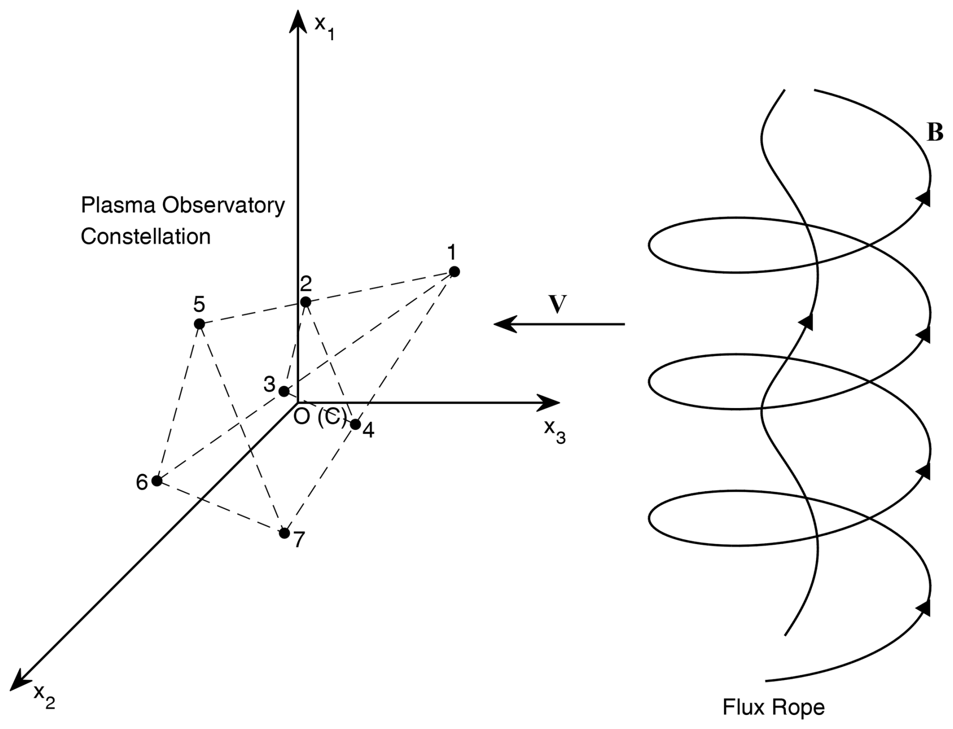
Figure 1 Schematic plot showing observation of a magnetic structure by the Plasma Observatory constellation, which is composed of seven spacecraft. (The special configuration is similar to the mission term proposal, and the actual geometry can deviate from it.) Barycentric coordinates are adopted; thus, the center C of the constellation overlaps with the origin, O, of the Cartesian coordinates (x₁, x₂, x₃), the magnetic structure is assumed to be moving at velocity V relative to the constellation, and the x₃ axis is presumed to be anti-parallel to V.

The following transformation relationship involving the mixed space–time derivatives is used for the magnetic measurements:

$$\begin{array}{}\text{(3)}& {\partial }_t\mathit{B}=-\mathit{V}\cdot \mathbf{\nabla }\mathit{B}\text{and}{\partial }_t\mathbf{\nabla }\mathit{B}=-\mathit{V}\cdot \mathbf{\nabla }\mathbf{\nabla }\mathit{B}.\end{array}$$

By computing the temporal derivative, ∂_tB, and then the temporal derivative of spatial gradient ∂_t∇B, this relationship allows both the apparent velocity, V, of the magnetic structure and the nine components of the quadratic magnetic gradient tensor along the direction of motion, $\widehat{\mathit{V}}\cdot \mathbf{\nabla }\mathbf{\nabla }\mathit{B}$, to be obtained (Shen et al., 2021a). The constraints to Eq. (3) are that the plasmas are highly conductive and have a very low velocity ($\mathit{V}/c\ll \mathrm{1}$, where V is the apparent speed of the magnetic structure and c is the speed of light in a vacuum) and that the physical processes are slowly evolving at low frequencies. The truncation errors in Eq. (3) are on the order of $\mathit{V}/c$.

2.1.1 The zeroth iteration

First, the temporal variation rate ∂_tB and first-order magnetic gradient (∇B)⁽⁰⁾, where the uppercase label (0) denotes the zeroth order, can be obtained from seven- or nine-point simultaneous magnetic measurements. Here, the change rate of the magnetic field can be obtained from the temporal (time series) measurements at each spacecraft. The linear spatial gradient can be obtained using four-spacecraft techniques (Chanteur, 1998; Harvey, 1998; Shen et al., 2003). Using Eq. (3), we can thus obtain the apparent velocity, V, of the magnetic structure (Shen et al., 2021a). Next, the longitudinal components of the second-order magnetic gradient, $\widehat{\mathit{V}}\cdot \mathbf{\nabla }\mathbf{\nabla }\mathit{B}=\frac{\mathrm{1}}{V}{\partial }_{\mathrm{3}}\mathbf{\nabla }\mathit{B}$, can be deduced from the transformation relationship (Eq. 3). These steps are described in detail in Sect. 2.2.1. Finally, the remaining nine components of the second-order magnetic gradient (i.e., the transverse component, $G_{rs}^{\left(\mathrm{1}\right)}={\left({\mathrm{\nabla }}_r{\mathrm{\nabla }}_{s}f\right)}^{\left(\mathrm{1}\right)}$, where r, $s=\mathrm{1},\mathrm{2}$) can be determined from the seven- or nine-point simultaneous magnetic measurements using the least-squares method, allowing for a first-order quadratic magnetic gradient, (∇∇B)⁽¹⁾, to be obtained, as described next.

2.1.2 The first-order iteration

Provided with the first-order quadratic magnetic gradient, (∇∇B)⁽¹⁾, the corrected first-order linear magnetic gradient, (∇B)⁽¹⁾, can be found using the least-squares method. Furthermore, the corrected apparent velocity, V⁽¹⁾, of the magnetic structure and the longitudinal components of the second-order quadratic magnetic gradient, ${\left(\widehat{\mathit{V}}\cdot \mathbf{\nabla }\mathbf{\nabla }\mathit{B}\right)}^{\left(\mathrm{2}\right)}$, can be obtained from the transformation relationship (Eq. 3). Again, the corrected transverse components of the quadratic magnetic gradient $(G_{rs}^{\left(\mathrm{2}\right)},r,s=\mathrm{1},\mathrm{2})$ are obtained using the least-squares method, allowing a second-order quadratic magnetic gradient (∇∇B)⁽²⁾ to be obtained.

The iterations are performed repeatedly until results converge, which means satisfactory results have been achieved.

For the 7S/C Plasma Observatory, the seven-point magnetic measurements in 3-D yield 7 × 3 = 21 independent parameters, while the reference frame transformation provides nine constraints, resulting in $\mathrm{21}+\mathrm{9}=\mathrm{30}$ input parameters in total. The objective is to determine the magnetic field (3 parameters), first-order gradient (9 parameters), and quadratic magnetic gradient (18 parameters) at the mesocenter of the constellation, a total of $\mathrm{3}+\mathrm{9}+\mathrm{18}=\mathrm{30}$ parameters. Therefore, this scheme is reasonable and such that the solution to the system of equations can be uniquely determined.

Clearly, the 9S/C magnetic measurements of HelioSwarm are sufficient to draw first-order and quadratic magnetic gradients using this method. These results indicate that the developed method is suitable for constellations comprising at least seven spacecraft.

2.2 Practical steps of the algorithm

Details of the steps used are given below.

2.2.1 The zeroth iteration

We first assume a linear approximation in space and let $G_{ij}^{\left(\mathrm{0}\right)}=\mathrm{0}$. The magnetic field, ${\mathit{B}}_c^{\left(\mathrm{0}\right)}$, and its linear gradient, (∇B)⁽⁰⁾, at the mesocenter of the constellation can then be obtained using the following formulas (Harvey, 1998; Shen et al., 2003):

$$\begin{array}{}\text{(4)}& {\displaystyle }{B}_{ci}^{\left(\mathrm{0}\right)}={\displaystyle \frac{\mathrm{1}}{N}}\sum _{\mathit{\alpha }=\mathrm{1}}^N{B}_{\mathit{\alpha }i},\text{(5)}& {\displaystyle }{\left({\partial }_i{B}_j\right)}_c^{\left(\mathrm{0}\right)}={\displaystyle \frac{\mathrm{1}}{N}}\sum _{\mathit{\alpha }=\mathrm{1}}^N{B}_{\mathit{\alpha }i}{r}_{\mathit{\alpha }k}{R}_{kj}^{-\mathrm{1}},\end{array}$$

where the volume tensor is $R_{kj}=\frac{\mathrm{1}}{N}\sum _{\mathit{\alpha }=\mathrm{1}}^N{r}_{\mathit{\alpha }k}{r}_{\mathit{\alpha }j}$ or $\mathbf{R}\equiv \frac{\mathrm{1}}{N}\sum _{\mathit{\alpha }=\mathrm{1}}^N{\mathit{r}}_{\mathit{\alpha }}{\mathit{r}}_{\mathit{\alpha }}$, where N is the number of spacecraft within the constellation and $R_{kj}^{-\mathrm{1}}$ is the inverse of the volume tensor R_kj. The determinant of the volume tensor is required to be nonzero, i.e., $R=\det \left(R_{kj}\right)\ne \mathrm{0}$. This is equivalent to the constellation being nonplanar (i.e., not all spacecraft are on the same plane).

The temporal variation rate, ${\left({\partial }_t\mathit{B}\right)}_c^{\left(\mathrm{0}\right)}$, is readily obtained from central differences in the magnetic observation time series. Now the frame transformation relationship, Eq. (3), is reduced to the apparent velocity, V⁽⁰⁾, of the magnetic structure and the longitudinal components of the quadratic magnetic gradient ${\left({\partial }_{\mathrm{3}}\mathbf{\nabla }\mathit{B}\right)}^{\left(\mathrm{1}\right)}$.

First, the zeroth approximation of the apparent velocity of the magnetic structure V⁽⁰⁾ can be found using the frame transformation relationship:

$$\begin{array}{}\text{(6)}& {\left({\partial }_t\mathit{B}\right)}^{\left(\mathrm{0}\right)}=-{\mathit{V}}^{\left(\mathrm{0}\right)}\cdot {\left(\mathbf{\nabla }\mathit{B}\right)}^{\left(\mathrm{0}\right)}.\end{array}$$

Then, using the relationship

$$\begin{array}{}\text{(7)}& {\partial }_t{\left(\mathbf{\nabla }\mathit{B}\right)}^{\left(\mathrm{0}\right)}=-{\mathit{V}}^{\left(\mathrm{0}\right)}\cdot {\left(\mathbf{\nabla }\mathbf{\nabla }\mathit{B}\right)}^{\left(\mathrm{1}\right)},\end{array}$$

the longitude component of the quadratic magnetic gradient at the first order can be derived as follows:

$$\begin{array}{}\text{(8)}& {\left({\partial }_{\mathrm{3}}\mathbf{\nabla }\mathit{B}\right)}_c^{\left(\mathrm{1}\right)}={\displaystyle \frac{\mathrm{1}}{V^{\left(\mathrm{0}\right)}}}{\partial }_t{\left(\mathbf{\nabla }\mathit{B}\left(t,{\mathit{r}}_c\right)\right)}^{\left(\mathrm{0}\right)},\end{array}$$

which is just $\left(G_{\mathrm{31}}^{\left(\mathrm{1}\right)},G_{\mathrm{32}}^{\left(\mathrm{1}\right)},G_{\mathrm{33}}^{\left(\mathrm{1}\right)}\right)$.

The remaining components of the quadratic magnetic gradients can be deduced using the least-squares method.

We assume that the following applies:

$$\begin{array}{}\text{(9)}& S={\displaystyle \frac{\mathrm{1}}{N}}\sum _{\mathit{\alpha }=\mathrm{1}}^N{\left[f_c^{\left(\mathrm{0}\right)}+x_{\left(\mathit{\alpha }\right)}^i{g}_i^{\left(\mathrm{0}\right)}+{\displaystyle \frac{\mathrm{1}}{\mathrm{2}}}{x}_{\left(\mathit{\alpha }\right)}^i{x}_{\left(\mathit{\alpha }\right)}^j{G}_{ij}^{\left(\mathrm{1}\right)}-f_{\left(\mathit{\alpha }\right)}\right]}^{\mathrm{2}},\end{array}$$

which can also be written as

$$\begin{array}{}\text{(10)}& \begin{array}{rl}S& ={\displaystyle \frac{\mathrm{1}}{N}}\sum _{\mathit{\alpha }=\mathrm{1}}^N[f_c^{\left(\mathrm{0}\right)}+x_{\left(\mathit{\alpha }\right)}^i{g}_i^{\left(\mathrm{0}\right)}-f_{\left(\mathit{\alpha }\right)}\\ & +\left(\mathrm{1}-{\displaystyle \frac{\mathrm{1}}{\mathrm{2}}}{\mathit{\delta }}_{\mathrm{i}\mathrm{3}}\right)x_{\left(\mathit{\alpha }\right)}^i{x}_{\left(\mathit{\alpha }\right)}^{\mathrm{3}}{G}_{i\mathrm{3}}^{\left(\mathrm{1}\right)}+{\displaystyle \frac{\mathrm{1}}{\mathrm{2}}}{x}_{\left(\mathit{\alpha }\right)}^p{x}_{\left(\mathit{\alpha }\right)}^q{G}_{pq}^{\left(\mathrm{1}\right)}{]}^{\mathrm{2}}.\end{array}\end{array}$$

where $p,q=\mathrm{1},\mathrm{2}$.

If δS=0, then

$$\begin{array}{}\text{(11)}& \begin{array}{rl}{\displaystyle \frac{\partial S}{\partial G_{pq}}}& ={\displaystyle \frac{\mathrm{1}}{N}}\sum _{\mathit{\alpha }=\mathrm{1}}^N\mathrm{2}[f_c^{\left(\mathrm{0}\right)}+x_{\left(\mathit{\alpha }\right)}^i{g}_i^{\left(\mathrm{0}\right)}-f_{\left(\mathit{\alpha }\right)}\\ & +\left(\mathrm{1}-{\displaystyle \frac{\mathrm{1}}{\mathrm{2}}}{\mathit{\delta }}_{i\mathrm{3}}\right)x_{\left(\mathit{\alpha }\right)}^i{x}_{\left(\mathit{\alpha }\right)}^{\mathrm{3}}{G}_{i\mathrm{3}}^{\left(\mathrm{1}\right)}+{\displaystyle \frac{\mathrm{1}}{\mathrm{2}}}{x}_{\left(\mathit{\alpha }\right)}^r{x}_{\left(\mathit{\alpha }\right)}^s{G}_{rs}^{\left(\mathrm{1}\right)}]\\ & \cdot x_{\left(\mathit{\alpha }\right)}^p{x}_{\left(\mathit{\alpha }\right)}^q=\mathrm{0},\end{array}\end{array}$$

which reduces to

$$\begin{array}{}\text{(12)}& \begin{array}{rl}& f_c^{\left(\mathrm{0}\right)}\sum _{\mathit{\alpha }=\mathrm{1}}^N{x}_{\left(\mathit{\alpha }\right)}^p{x}_{\left(\mathit{\alpha }\right)}^q+\sum _{\mathit{\alpha }=\mathrm{1}}^N{x}_{\left(\mathit{\alpha }\right)}^i{x}_{\left(\mathit{\alpha }\right)}^p{x}_{\left(\mathit{\alpha }\right)}^q{g}_i^{\left(\mathrm{0}\right)}\\ & -\sum _{\mathit{\alpha }=\mathrm{1}}^N{f}_{\left(\mathit{\alpha }\right)}{x}_{\left(\mathit{\alpha }\right)}^p{x}_{\left(\mathit{\alpha }\right)}^q\\ & +\sum _{\mathit{\alpha }=\mathrm{1}}^N\left(\mathrm{1}-{\displaystyle \frac{\mathrm{1}}{\mathrm{2}}}{\mathit{\delta }}_{\mathrm{i}\mathrm{3}}\right)x_{\left(\mathit{\alpha }\right)}^i{x}_{\left(\mathit{\alpha }\right)}^{\mathrm{3}}{x}_{\left(\mathit{\alpha }\right)}^p{x}_{\left(\mathit{\alpha }\right)}^q{G}_{i\mathrm{3}}^{\left(\mathrm{1}\right)}\\ & +{\displaystyle \frac{\mathrm{1}}{\mathrm{2}}}\sum _{\mathit{\alpha }=\mathrm{1}}^N{x}_{\left(\mathit{\alpha }\right)}^r{x}_{\left(\mathit{\alpha }\right)}^s{x}_{\left(\mathit{\alpha }\right)}^p{x}_{\left(\mathit{\alpha }\right)}^q{G}_{rs}^{\left(\mathrm{1}\right)}=\mathrm{0},\end{array}\end{array}$$

resulting in $G_{rs}^{\left(\mathrm{1}\right)}\left(r,s=\mathrm{1},\mathrm{2}\right)$, i.e., $\left(G_{\mathrm{21}}^{\left(\mathrm{1}\right)},G_{\mathrm{22}}^{\left(\mathrm{1}\right)},G_{\mathrm{11}}^{\left(\mathrm{1}\right)}\right)$. The constellation must be nonplanar to achieve this result. This is verified as follows.

Following Zhou and Shen (2024), in order for the solution to exist, it is expected that the position of all the spacecraft in the constellation must not obey the following formula:

$$\begin{array}{}\text{(13)}& \begin{array}{rl}& a_{\mathrm{11}}{\left(x_{\left(\mathit{\alpha }\right)}^{\mathrm{1}}\right)}^{\mathrm{2}}+a_{\mathrm{12}}{x}_{\left(\mathit{\alpha }\right)}^{\mathrm{1}}{x}_{\left(\mathit{\alpha }\right)}^{\mathrm{2}}+a_{\mathrm{12}}{x}_{\left(\mathit{\alpha }\right)}^{\mathrm{2}}{x}_{\left(\mathit{\alpha }\right)}^{\mathrm{1}}\\ & +a_{\mathrm{22}}{\left(x_{\left(\mathit{\alpha }\right)}^{\mathrm{2}}\right)}^{\mathrm{2}}=\mathrm{0},\end{array}\end{array}$$

where $a_{rs}\left(r,s=\mathrm{1},\mathrm{2}\right)$ is a set of fixed coefficients. The above equations can be rewritten as follows:

$$\begin{array}{}\text{(14)}& a_{\mathrm{11}}{\left(x_{\left(\mathit{\alpha }\right)}^{\mathrm{1}}/x_{\left(\mathit{\alpha }\right)}^{\mathrm{2}}\right)}^{\mathrm{2}}+\mathrm{2}{a}_{\mathrm{12}}\left(x_{\left(\mathit{\alpha }\right)}^{\mathrm{1}}/x_{\left(\mathit{\alpha }\right)}^{\mathrm{2}}\right)+a_{\mathrm{22}}=\mathrm{0},\end{array}$$

which reduces to $x_{\left(\mathit{\alpha }\right)}^{\mathrm{1}}/x_{\left(\mathit{\alpha }\right)}^{\mathrm{2}}=\mathrm{constant}$. It means that all the spacecraft are in the plane parallel to the x₃ axis or the motion direction. Therefore, it is necessary to have the constellation not be planar in order to deduce the quadratic magnetic gradients as well as the linear magnetic gradient. The next iterations would also require this condition.

2.2.2 First-order iteration

Assuming that

$$\begin{array}{}\text{(15)}& S={\displaystyle \frac{\mathrm{1}}{N}}\sum _{\mathit{\alpha }=\mathrm{1}}^N{\left[f_c^{\left(\mathrm{1}\right)}+x_{\left(\mathit{\alpha }\right)}^i{g}_i^{\left(\mathrm{1}\right)}+{\displaystyle \frac{\mathrm{1}}{\mathrm{2}}}{x}_{\left(\mathit{\alpha }\right)}^i{x}_{\left(\mathit{\alpha }\right)}^j{G}_{ij}^{\left(\mathrm{1}\right)}-f_{\left(\mathit{\alpha }\right)}\right]}^{\mathrm{2}},\end{array}$$

if δS=0, then

$$\begin{array}{}\text{(16)}& {\displaystyle \frac{\partial S}{\partial f_c^{\left(\mathrm{1}\right)}}}=\mathrm{0},{\displaystyle \frac{\partial S}{\partial g_i^{\left(\mathrm{1}\right)}}}=\mathrm{0}.\end{array}$$

From $\frac{\partial S}{\partial f_c^{\left(\mathrm{1}\right)}}=\mathrm{0}$, it can be assumed that

$$\begin{array}{}\text{(17)}& {\displaystyle \frac{\mathrm{1}}{N}}\sum _{\mathit{\alpha }=\mathrm{1}}^N\left[f_c^{\left(\mathrm{1}\right)}+x_{\left(\mathit{\alpha }\right)}^i{g}_i^{\left(\mathrm{1}\right)}+{\displaystyle \frac{\mathrm{1}}{\mathrm{2}}}{x}_{\left(\mathit{\alpha }\right)}^i{x}_{\left(\mathit{\alpha }\right)}^j{G}_{ij}^{\left(\mathrm{1}\right)}-f_{\left(\mathit{\alpha }\right)}\right]=\mathrm{0},\end{array}$$

meaning that

$$\begin{array}{}\text{(18)}& \begin{array}{rl}{f}_c^{\left(\mathrm{1}\right)}& ={\displaystyle \frac{\mathrm{1}}{N}}\sum _{\mathit{\alpha }=\mathrm{1}}^N{f}_{\left(\mathit{\alpha }\right)}-{\displaystyle \frac{\mathrm{1}}{\mathrm{2}N}}\sum _{\mathit{\alpha }=\mathrm{1}}^N{x}_{\left(\mathit{\alpha }\right)}^i{x}_{\left(\mathit{\alpha }\right)}^j{G}_{ij}^{\left(\mathrm{1}\right)}\\ & ={\displaystyle \frac{\mathrm{1}}{N}}\sum _{\mathit{\alpha }=\mathrm{1}}^N{f}_{\left(\mathit{\alpha }\right)}-{\displaystyle \frac{\mathrm{1}}{\mathrm{2}}}{R}^{ij}{G}_{ij}^{\left(\mathrm{1}\right)}.\end{array}\end{array}$$

If $\frac{\partial S}{\partial g_i^{\left(\mathrm{1}\right)}}=\mathrm{0}$, this can be reduced to

$$\begin{array}{}\text{(19)}& \begin{array}{rl}& {\displaystyle \frac{\mathrm{1}}{N}}\sum _{\mathit{\alpha }=\mathrm{1}}^N[f_c^{\left(\mathrm{1}\right)}+x_{\left(\mathit{\alpha }\right)}^i{g}_i^{\left(\mathrm{1}\right)}+{\displaystyle \frac{\mathrm{1}}{\mathrm{2}}}{x}_{\left(\mathit{\alpha }\right)}^i{x}_{\left(\mathit{\alpha }\right)}^j{G}_{ij}^{\left(\mathrm{1}\right)}\\ & -f_{\left(\mathit{\alpha }\right)}]x_{\left(\mathit{\alpha }\right)}^k=\mathrm{0},\end{array}\end{array}$$

i.e., the following applies:

$$\begin{array}{}\text{(20)}& \begin{array}{rl}& {\displaystyle \frac{\mathrm{1}}{N}}\sum _{\mathit{\alpha }=\mathrm{1}}^N{x}_{\left(\mathit{\alpha }\right)}^k{x}_{\left(\mathit{\alpha }\right)}^i{g}_i^{\left(\mathrm{1}\right)}+{\displaystyle \frac{\mathrm{1}}{\mathrm{2}}}{\displaystyle \frac{\mathrm{1}}{N}}\sum _{\mathit{\alpha }=\mathrm{1}}^N{x}_{\left(\mathit{\alpha }\right)}^k{x}_{\left(\mathit{\alpha }\right)}^i{x}_{\left(\mathit{\alpha }\right)}^j{G}_{ij}^{\left(\mathrm{1}\right)}\\ & -{\displaystyle \frac{\mathrm{1}}{N}}\sum _{\mathit{\alpha }=\mathrm{1}}^N{f}_{\left(\mathit{\alpha }\right)}{x}_{\left(\mathit{\alpha }\right)}^k=\mathrm{0}.\end{array}\end{array}$$

The tensor $R^{kij}=\frac{\mathrm{1}}{N}\sum _{\mathit{\alpha }=\mathrm{1}}^N{x}_{\left(\mathit{\alpha }\right)}^k{x}_{\left(\mathit{\alpha }\right)}^i{x}_{\left(\mathit{\alpha }\right)}^j$ is then defined, resulting in

$$\begin{array}{}\text{(21)}& R^{ki}{g}_i^{\left(\mathrm{1}\right)}+{\displaystyle \frac{\mathrm{1}}{\mathrm{2}}}{R}^{kij}{G}_{ij}^{\left(\mathrm{1}\right)}-{\displaystyle \frac{\mathrm{1}}{N}}\sum _{\mathit{\alpha }=\mathrm{1}}^N{f}_{\left(\mathit{\alpha }\right)}{x}_{\left(\mathit{\alpha }\right)}^k=\mathrm{0}.\end{array}$$

Therefore, the first magnetic gradient is

$$\begin{array}{}\text{(22)}& \begin{array}{rl}{g}_{\mathrm{\ell }}^{\left(\mathrm{1}\right)}& =-{\displaystyle \frac{\mathrm{1}}{\mathrm{2}}}{\left(R^{-\mathrm{1}}\right)}^{k\mathrm{\ell }}{R}^{kij}{G}_{ij}^{\left(\mathrm{1}\right)}\\ & +{\left(R^{-\mathrm{1}}\right)}^{k\mathrm{\ell }}\cdot {\displaystyle \frac{\mathrm{1}}{N}}\sum _{\mathit{\alpha }=\mathrm{1}}^N{f}_{\left(\mathit{\alpha }\right)}{x}_{\left(\mathit{\alpha }\right)}^k.\end{array}\end{array}$$

Using Eq. (3), it is now possible to obtain the corrected apparent velocity V⁽¹⁾ of the magnetic structure and the longitudinal components of the corrected quadratic magnetic gradient ${\left({\partial }_{\mathrm{3}}\mathbf{\nabla }\mathit{B}\right)}^{\left(\mathrm{2}\right)}\left({\left({\partial }_{\mathrm{3}}{\partial }_i\mathit{B}\right)}^{\left(\mathrm{2}\right)}\right)$ as in the zeroth iteration.

The least-squares method is then used to obtain the remaining nine components of the corrected quadratic magnetic gradient.

If

$$\begin{array}{}\text{(23)}& \begin{array}{rl}S& ={\displaystyle \frac{\mathrm{1}}{N}}\sum _{\mathit{\alpha }=\mathrm{1}}^N{\left[f_{\left(c\right)}^{\left(\mathrm{1}\right)}+x_{\left(\mathit{\alpha }\right)}^i{g}_i^{\left(\mathrm{1}\right)}+{\displaystyle \frac{\mathrm{1}}{\mathrm{2}}}{x}_{\left(\mathit{\alpha }\right)}^i{x}_{\left(\mathit{\alpha }\right)}^j{G}_{ij}^{\left(\mathrm{2}\right)}-f_{\left(\mathit{\alpha }\right)}\right]}^{\mathrm{2}}\\ & ={\displaystyle \frac{\mathrm{1}}{N}}\sum _{\mathit{\alpha }=\mathrm{1}}^N[f_c^{\left(\mathrm{1}\right)}+x_{\left(\mathit{\alpha }\right)}^i{g}_i^{\left(\mathrm{1}\right)}-f_{\left(\mathit{\alpha }\right)}\\ & +\left(\mathrm{1}-{\displaystyle \frac{\mathrm{1}}{\mathrm{2}}}{\mathit{\delta }}_{i\mathrm{3}}\right)x_{\left(\mathit{\alpha }\right)}^i{x}_{\left(\mathit{\alpha }\right)}^{\mathrm{3}}{G}_{i\mathrm{3}}^{\left(\mathrm{2}\right)}+{\displaystyle \frac{\mathrm{1}}{\mathrm{2}}}{x}_{\left(\mathit{\alpha }\right)}^p{x}_{\left(\mathit{\alpha }\right)}^q{G}_{pq}^{\left(\mathrm{2}\right)}{]}^{\mathrm{2}},\end{array}\end{array}$$

then $G_{pq}^{\left(\mathrm{2}\right)}\left(p,q=\mathrm{1},\mathrm{2}\right)$ can be obtained using the same procedure as that used for the zeroth iteration so that all the components of the corrected quadratic magnetic gradient (∇∇B)⁽²⁾ are obtained.

Similarly, two or more iterations can be performed until stable linear and second-order magnetic gradients are obtained.

This algorithm requires that the constellation be composed of at least seven spacecraft and that its configuration be nonplanar. Because both the 9S/C HelioSwarm and 7S/C Plasma Observatory satisfy these requirements, the linear and quadratic magnetic gradients can be readily obtained.

The curlometer technique (Dunlop et al., 2002b) is used to calculate the current density based on multiple spacecraft magnetic measurements, with the relative error estimated by the ratio between the divergence and the curl of the magnetic field, i.e., $\left|\frac{\mathbf{\nabla }\cdot \mathit{B}}{\mathbf{\nabla }\times \mathit{B}}\right|$. If the length and the magnetic field are normalized by the characteristic distance and magnetic strength (D,B₀), the equation becomes $\left|\frac{\stackrel{\mathrm{‾}}{\mathbf{\nabla }}\cdot \stackrel{\mathrm{‾}}{\mathit{B}}}{\stackrel{\mathrm{‾}}{\mathbf{\nabla }}\times \stackrel{\mathrm{‾}}{\mathit{B}}}\right|\approx \left|\frac{\stackrel{\mathrm{‾}}{\mathbf{\nabla }}\cdot \stackrel{\mathrm{‾}}{\mathit{B}}}{\mathrm{1}}\right|=\left|\stackrel{\mathrm{‾}}{\mathbf{\nabla }}\cdot \stackrel{\mathrm{‾}}{\mathit{B}}\right|$. Therefore, the dimensionless divergence of the magnetic field calculated with observation data can be regarded as a reasonable measure of the relative error within the linear magnetic gradient. Similarly, the dimensionless $\left|\stackrel{\mathrm{‾}}{\mathbf{\nabla }}{\left(\stackrel{\mathrm{‾}}{\mathbf{\nabla }}\cdot \stackrel{\mathrm{‾}}{\mathit{B}}\right)}_c\right|$ can be used as a measure that describes the relative error in the quadratic magnetic gradient derived using the method.

3 Comparison of new method with analytical modeling

In this section, the new method is applied to two analytical magnetic field models (a cylindrical force-free flux rope and a dipole magnetic field) to evaluate their validity and accuracy. The applicability of this approach was tested on the 7S/C Plasma Observatory (N=7) under the assumption that the seven-spacecraft cluster crosses a magnetic field structure (as illustrated in Fig. 1) by comparing the linear and quadratic gradients of the magnetic field obtained by the new method with those obtained by accurate modeling.

The positions of the seven spacecrafts in the barycentric coordinate system were generated randomly with Cartesian coordinates between −0.02 and 0.02 R_E, as seen in Table 1. The 7S/C array is illustrated in Fig. 2.

Table 1 Coordinates of the seven spacecraft in the barycenter coordinate system, with α denoting the spacecraft number.

Figure 2 Configuration of the 7S/C constellation.

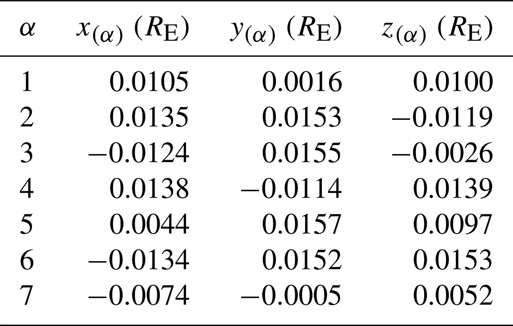
The characteristic configuration of the spacecraft is described using several parameters. The three eigenvalues of the volumetric tensor R^ij are represented by w₁, w₂, and w₃ (where $w_{\mathrm{1}}\ge w_{\mathrm{2}}\ge w_{\mathrm{3}}$) (Harvey, 1998), with their square roots representing the characteristic half-widths of the S/C in the three orthogonal directions along the corresponding eigenvectors (Harvey, 1998). The characteristic size of the S/C constellation is twice the square root of the maximum eigenvalue, $L=\mathrm{2}\sqrt{w_{\mathrm{1}}}$ (Robert et al., 1998; Shen et al., 2012). For the 7S/C constellation tested in this section, the three eigenvalues are $w_{\mathrm{1}}=\mathrm{0.1643}\times {\mathrm{10}}^{-\mathrm{3}}{R}_{\mathrm{E}}^{\mathrm{2}}$, $w_{\mathrm{2}}=\mathrm{0.1104}\times {\mathrm{10}}^{-\mathrm{3}}$ $R_{\mathrm{E}}^{\mathrm{2}}$, and $w_{\mathrm{3}}=\mathrm{0.0341}\times {\mathrm{10}}^{-\mathrm{3}}{R}_{\mathrm{E}}^{\mathrm{2}}$. The characteristic size is $L=\mathrm{2}\sqrt{w_{\mathrm{1}}}=\mathrm{0.0256}$ R_E =163.33 km.

3.1 Flux rope

The flux rope was assumed to be force-free and cylindrically symmetrical. The magnetic field of the flux rope can be described using the Helmholtz equation, for which Lundquist (1950) provided analytical solutions in terms of the Bessel functions.

$$\begin{array}{}\text{(24)}& B_r=\mathrm{0},B_{\mathit{\phi }}\left(r\right)=B_{\mathrm{0}}{J}_{\mathrm{1}}\left(\mathit{\alpha }r\right),B_z\left(r\right)=B_{\mathrm{0}}{J}_{\mathrm{0}}\left(\mathit{\alpha }r\right),\end{array}$$

where r is the radial distance from the centric axis; α is a constant, with $\mathrm{1}/\mathit{\alpha }$ representing the characteristic scale of the flux rope; B₀ is the peak axial field intensity; and J₀ and J₁ are the zeroth- and first-order Bessel functions of the first kind, respectively. For this test, we set B₀=60 nT and $\mathit{\alpha }=\mathrm{1}/R_{\mathrm{E}}$.

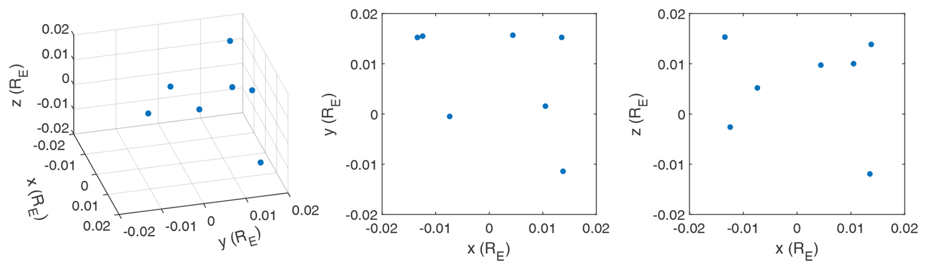
The 7S/C array was assumed to cross the flux rope in a straight line at uniform velocity. The array is represented by the barycenter with the red dot in Fig. 3 and moves from (−2, 0, 0) R_E to (2, 0, 0) R_E along the x axis over a time interval of 100 s. The resolution of the magnetic field measurement was set to 1 s for the time series observations, and the characteristic size of the 7S/C array was set to L=0.0256 R_E for the gradients of the magnetic field at the barycenter along the trajectory to be obtained.

Figure 3 The cylindrical force-free flux-rope crossing by the 7S/C constellation as viewed from the axial direction. The trajectory of the barycenter of the constellation from (−2, 0, 0) R_E to (2, 0, 0) R_E over 100 s is shown by the dotted red line. The blue lines represent magnetic field lines.

The linear gradient of the magnetic field (∇_iB_k) has 9 components, while the quadratic gradient (∇_i∇_jB_k) comprises 27 components. According to the analytical flux-rope model and symmetry of the quadratic gradients, only five independent components of the quadratic gradients ∇₁∇₂B₁, ∇₁∇₁B₂, ∇₂∇₂B₂, ∇₁∇₁B₃, and ∇₂∇₂B₃ and three components of the linear gradient, ∇₂B₁, ∇₁B₂, and ∇₁B₃, are nonzero points on the x axis when using Cartesian coordinates, simplifying the comparison between the gradients derived from the proposed method and the analytical model.

The impact of iteration on the results was investigated first, with the results at two different points used to demonstrate the variation in the relative errors under iteration, as illustrated in Fig. 4. The relative error is defined as $\left|\left(X_{\mathrm{algorithm}}-X_{\mathrm{accurate}}\right)/X_{\mathrm{accurate}}\right|\times \mathrm{100}$ %, where X_algorithm and X_accurate represent the algorithm gradients derived using the new method and accurate values from the analytical model at the barycenter, respectively. As shown in Fig. 4a and c, the linear gradients converged to certain values within 50 iterations, and the final relative errors were lower than 0.02 %. Figure 4b and d also indicate that the quadratic gradients converge. However, some quadratic gradients converged faster than others with fewer relative errors, and final relative errors of no more than 1.5 % were obtained after 100 iterations. The maximum number of iterations was set to 100; thus, the gradients could be derived with good accuracy.

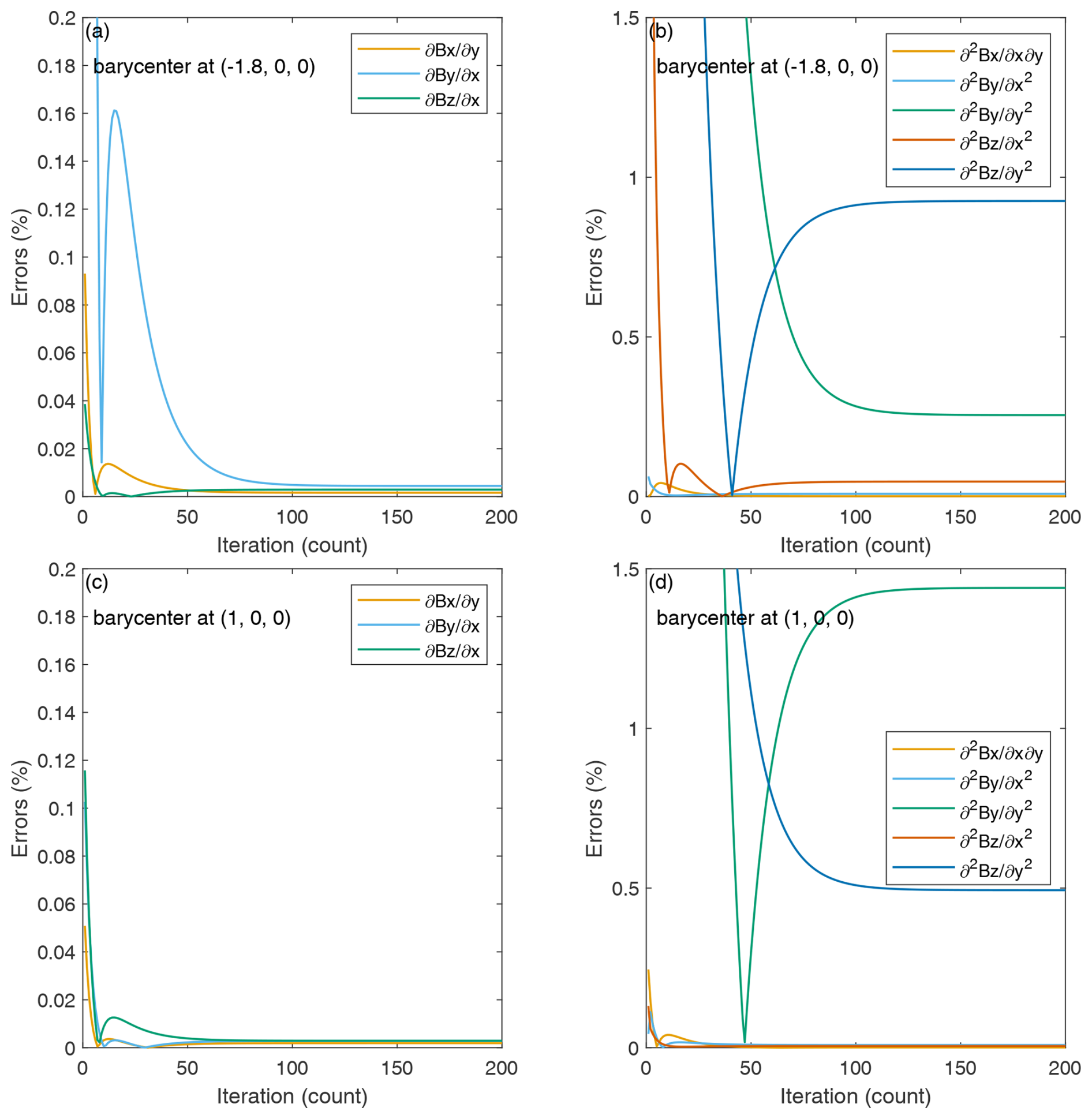
Figure 4 Relative errors in the nonzero components of the linear and quadratic gradients with different iteration numbers at various barycenters.

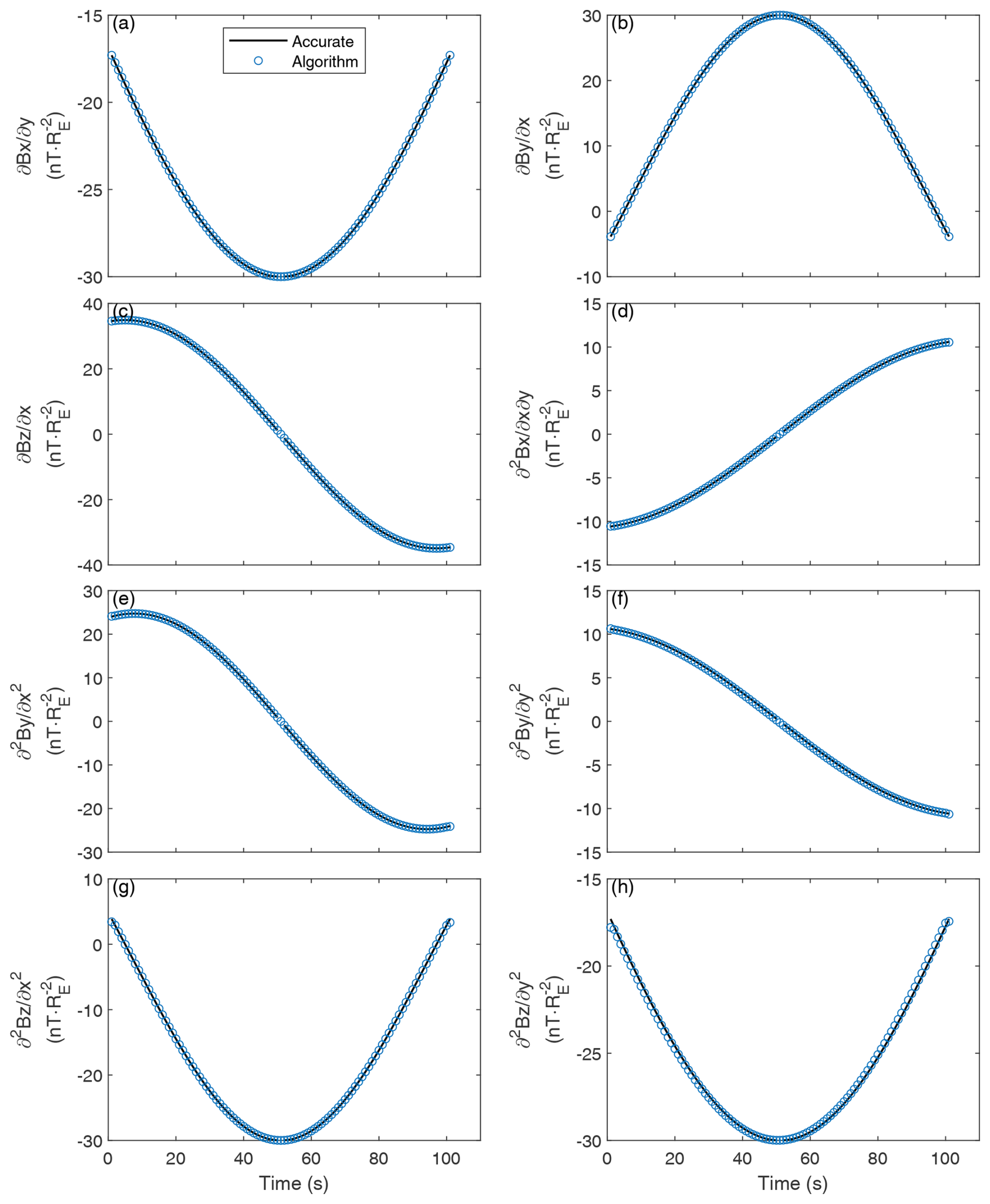
Figure 5 Time series showing nonzero components of the linear and quadratic gradients. Circles and solid lines represent the results obtained using the algorithm and accurate modeling, respectively.

Figure 5 shows a comparison of the nonzero linear and quadratic gradients at the barycenter derived from our method with those derived from the analytical model. The algorithm gradients are consistent with the accurate gradients, indicating that the proposed method is effective and precise when used with flux ropes.

Figure 6 Relative errors in the nonzero components of the linear and quadratic gradients along the crossing path.

The relative errors in the gradients at points along the trajectory are shown in Fig. 6. All the relative errors in the linear gradients were lower than 0.1 %, and the vast majority of the relative errors for the quadratic gradients did not exceed 5 %. It should be noted that the barycenter is at (0, 0, 0) at 50 s and that the nonzero components of the linear and quadratic gradients do not exist at (0, 0, 0). The barycenter is at (−0.04, 0, 0) R_E at 49 s, when accurate modeling and algorithm values for the quadratic gradient ∇₂∇₂B₂ are 0.3 and 0.1570 nT $R_{\mathrm{E}}^{-\mathrm{2}}$, respectively. The relative error approaches 50%; however, the absolute error is just 0.143 nT $R_{\mathrm{E}}^{-\mathrm{2}}$, which is approaching zero. Symmetrically, the situation described is the same as it would be if the barycenter were at (0.04, 0, 0).

3.2 Dipole field

The proposed method was also tested and verified using a magnetic dipole field. The geomagnetic dipole field is mathematically expressed as

$$\begin{array}{}\text{(25)}& \left\{\begin{array}{l}{B}_x=-\frac{\mathrm{3}xz}{r^{\mathrm{5}}}{B}_{\mathrm{0}}\\ B_y=-\frac{\mathrm{3}yz}{r^{\mathrm{5}}}{B}_{\mathrm{0}}\\ B_z=\frac{r^{\mathrm{2}}-\mathrm{3}{z}^{\mathrm{2}}}{r^{\mathrm{5}}}{B}_{\mathrm{0}}\end{array}\right.,\end{array}$$

where B₀ is the magnetic field at the Earth's Equator and is defined by $B_{\mathrm{0}}=\frac{{\mathit{\mu }}_{\mathrm{0}}M}{\mathrm{4}\mathit{\pi }{R}_{\mathrm{E}}^{\mathrm{3}}}=\mathrm{30}\mathrm{008}$ nT; $M=\mathrm{7.76}\times {\mathrm{10}}^{\mathrm{22}}$ A m² is the geomagnetic moment, with its direction set anti-parallel to the z axis; x, y, and z are the coordinates of the field points measured by R_E; and $r=\sqrt{x^{\mathrm{2}}+y^{\mathrm{2}}+z^{\mathrm{2}}}$ is the radial distance from the origin measured by R_E.

The 7S/C array was assumed to cross the dipole field in a straight line at constant velocity, with the barycenter parallel to the x axis and moving from (−5, 0, 5) R_E to (5, 0, 5) R_E over 125 s, as illustrated in Fig. 7. The resolution of the magnetic field measurement was set to 1 s, and the characteristic size of the 7S/C array was set to 0.0256 R_E, which is the same as that of the flux-rope case, for the gradients of the magnetic field at the barycenter along the trajectory to be obtained.

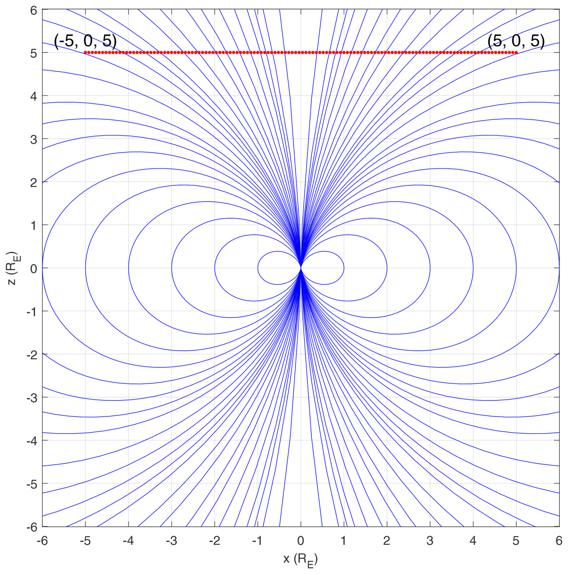
Figure 7 The magnetic dipole field crossed by the 7S/C array. Trajectory of the barycenter of the 7S/C array is from (−5, 0, 5) R_E to (5, 0, 5) R_E over 126 s as shown by the dotted red line. Blue lines represent magnetic field lines.

Only nonzero independent components are displayed, similarly to the flux-rope case. In view of the mathematical expression of the dipole field, 10 independent components of the quadratic gradients and 4 independent components of the linear gradients were nonzero along the crossing path.

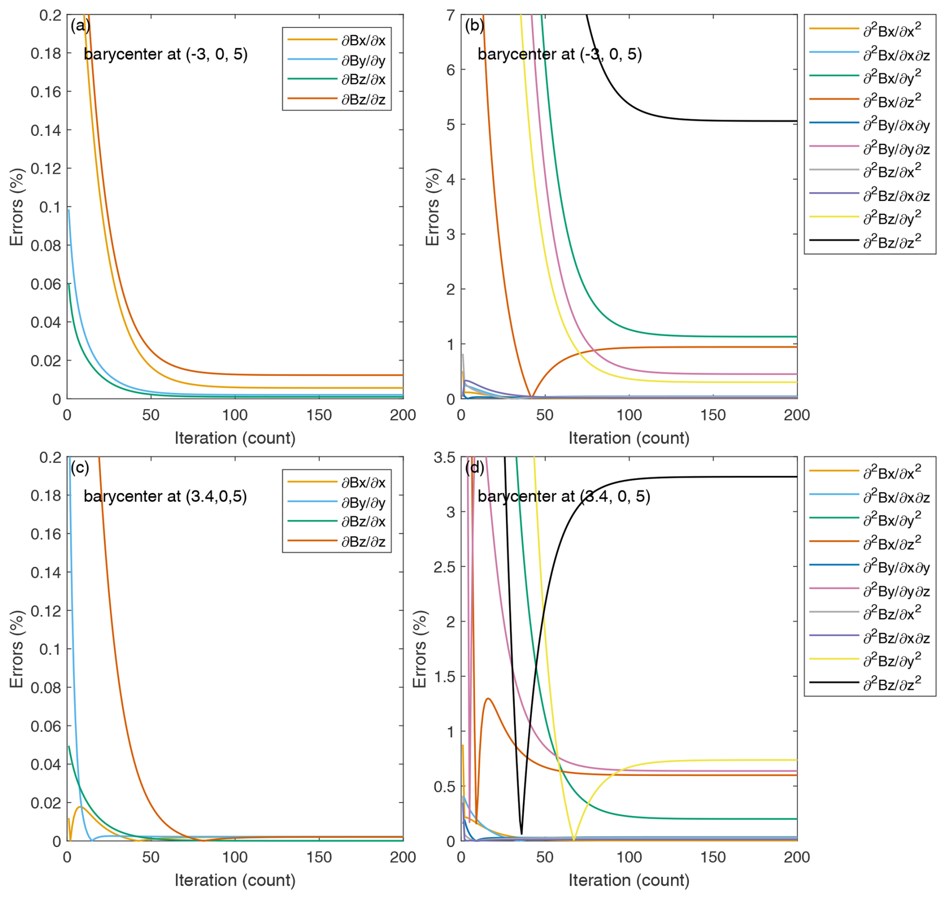
Figure 8 Relative errors in the nonzero components of the linear and quadratic gradients with different iteration numbers at various barycenters.

Figure 8 shows the variation in the relative errors under iteration at two different points. As shown in Fig. 8a and c, the linear gradients converged to certain values within 60 iterations, with final relative errors of less than 0.02 %. Figure 8b and d show that the quadratic gradients also converge to low errors. After 100 iterations, most of the relative errors in the quadratic gradients were lower than 1 %, and the largest relative error was no more than 6 %. These results suggest that it is reasonable to set the maximum number of iterations to 100 for the gradients to be derived with good accuracy in this case.

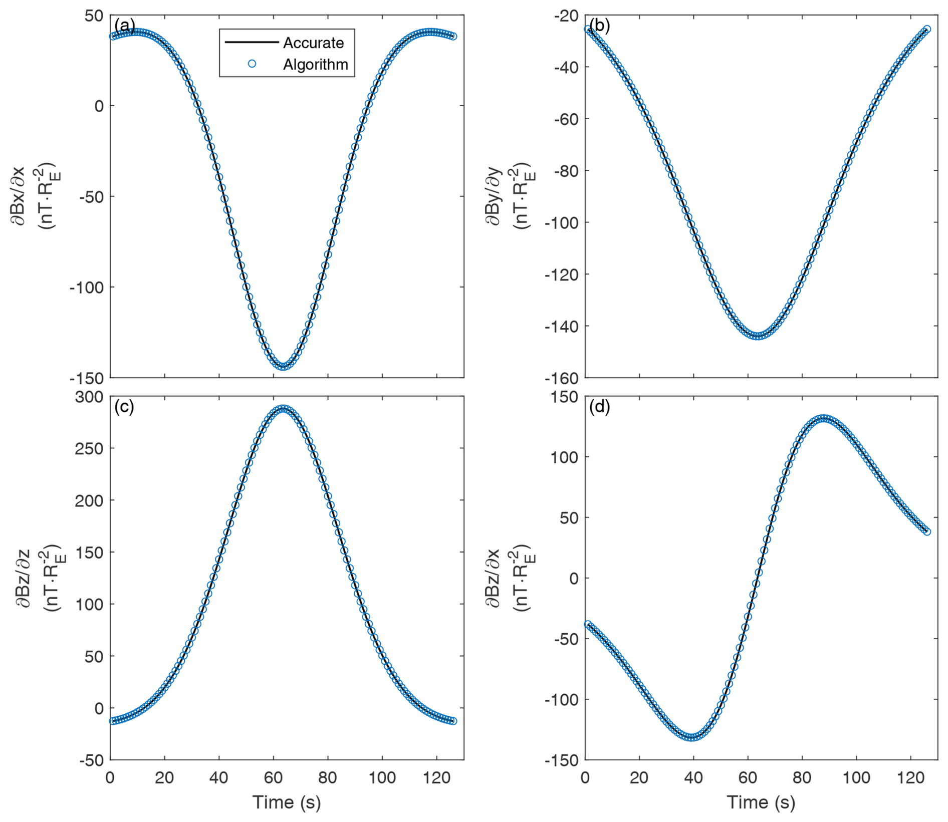
Figure 9 Time series showing nonzero components of the linear gradients. Circles and solid lines represent the results obtained using the algorithm and accurate modeling, respectively.

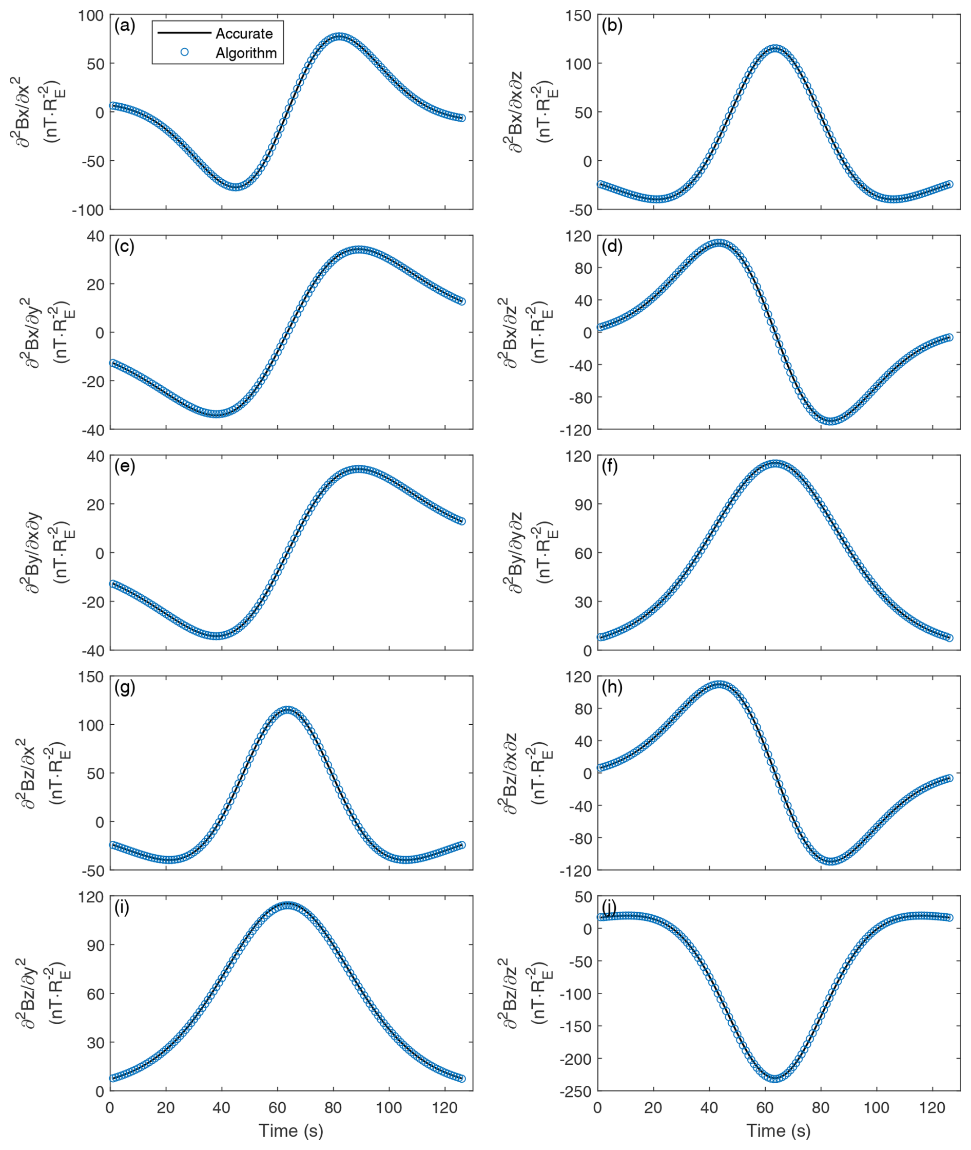
Figure 10 Time series showing nonzero components of the quadratic gradients. Circles and solid lines represent the results obtained using the algorithm and accurate modeling, respectively.

Figure 9 shows a comparison between the nonzero linear gradients derived from our method and those derived from the analytical model. A comparison between the nonzero quadratic gradients derived from the different sources is shown in Fig. 10. Both Figs. 9 and 10 indicate that the algorithm gradients are entirely consistent with those obtained from the accurate model, suggesting that the developed method is effective and precise for use with the dipole field.

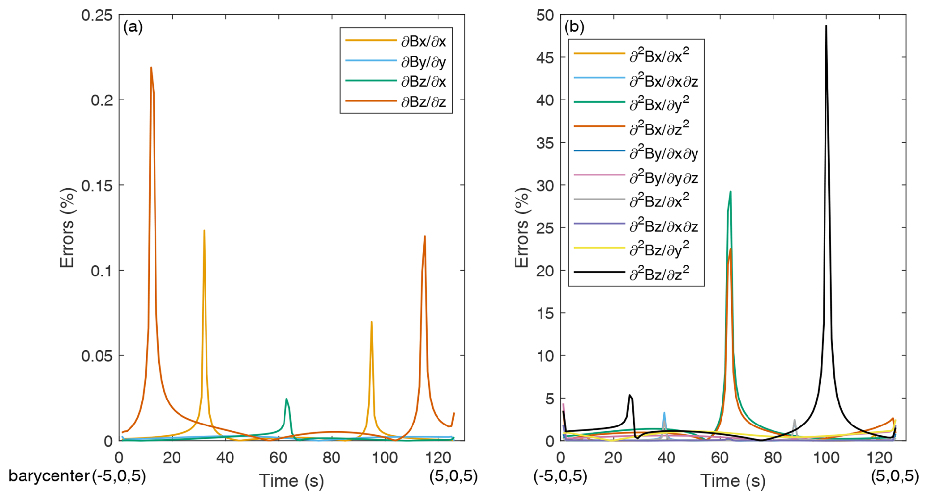
Figure 11 Relative errors in the nonzero components of the linear and quadratic gradients along the crossing path.

Figure 11 shows the relative errors in the gradients at the measured points along the crossing path. All the relative errors for the linear gradients were lower than 0.25 %, and most of the relative errors in the quadratic gradients were lower than 5 %. It should be noted that the barycenter is at (2.92, 0, 5) R_E at 100 s and the accurate and algorithm quadratic gradient ∇₃∇₃B₃ is −1.2584 and −0.6461 nT $R_{\mathrm{E}}^{-\mathrm{2}}$, respectively. The relative error approaches 50 %; however, the absolute error is 0.6123 nT $R_{\mathrm{E}}^{-\mathrm{2}}$, which is approaching zero. The barycenter is at (−0.04, 0, 5) R_E at 63 s and (0.04, 0, 5) R_E at 64 s. Similarly, the absolute errors in the quadratic gradients ∇₂∇₂B₁ and ∇₃∇₃B₁ were no more than 1 nT $R_{\mathrm{E}}^{-\mathrm{2}}$, whereas the relative errors were approximately 30 %.

3.3 Discussion

The two analytical magnetic field models (cylindrical force-free flux rope and dipole magnetic field) are simplified and highly symmetrical structures. The linear gradient of the magnetic field has 9 components, while the quadratic gradients comprise 18 independent components due to the symmetry of quadratic gradients. For the flux-rope case, only three components of linear gradient and five components of quadratic gradients have been assessed. But for the dipole-field case, 4 components of linear gradient and 10 components of quadratic gradients have been assessed. The number of assessed parameters has reached half. However, only a subset of the $\mathrm{9}+\mathrm{18}=\mathrm{27}$ components can be assessed. In this study, we have chosen a symmetric model magnetic field in order to easily compare our results with the analytic calculations. The zero components of the magnetic gradients are calculated with the algorithm and checked. Further evaluation of the algorithm with a less symmetric magnetosphere model could be useful.

4 Errors

In this section, we consider the diverse sources of errors – namely, the truncation error, discretization error, iteration error, and measurement error or random error – that can impact the linear and quadratic magnetic spatial gradient estimation. We introduce and discuss them as follows. Further detailed analyses can be found in Appendices A–D.

Discretization errors arise from the spatial resolution of measurement, which is the combined effect of finite temporal resolution and the relative motion of a probe with respect to the magnetic structure during the measurement period. The significance of these errors can be assessed by comparing the spatial resolution – due to S/C motion during the measurement or the S/C motion in between two successive measurements – with the separation between probes, over which the measured data are subtracted from one another. Typically, spacecraft separation within a constellation ranges from several hundred kilometers to several thousand kilometers, while the temporal resolution of magnetic measurement Δt is about 0.01 s, i.e., Δt=0.01 s. Assuming a magnetic structure moves at a velocity of V<500 km s⁻¹ relative to the spacecraft, the spatial resolution along the motion direction is about vΔt<5 km, which is significantly smaller than the S/C separation. Therefore, the corresponding discretization errors are expected to be small.

The iterative method provides converging solutions with decreasing errors as the number of iterations increases as demonstrated in Sect. 3. A particular type of error is the mismatch between the actual limit of the procedure and the approximation reached after a finite number of iterations. This error may be termed the iteration error. We note that it is not associated with the finite resolution of the spacecraft array or the time series. As shown in Fig. 4, the iterative procedures help reduce the calculation error and make the calculation more stable. In addition, once the number of iterations is sufficient (e.g., above 100), the iterative error becomes rather insignificant (see Appendix B).

Due to noise or measurement inaccuracies of input data, the estimated parameters (first and second derivatives) will be subject to random errors. The noise or disturbances in the data can come from the measurement error or the presence of high-frequency (physical) fluctuations, such as those from plasma waves, which can make the calculation of the high-order magnetic gradients very difficult (Shen et al., 2021a). When analyzing the actual observation data, filtering methods should be employed to remove the high-frequency components and avoid the negative effect of the noise. This process would help to extract large-scale magnetic structures under the consideration.

As discussed above, the discretization error and iteration error are expected to be rather small for the magnetic configuration considered. The errors caused by the random measurement errors would be large, and the global features of the magnetic structure would be missed (Shen et al., 2021a). In the following, only the truncation error has been evaluated.

In Sect. 3, the relative error is used to evaluate the truncation error of the proposed method. However, in some cases, evaluation with the relative error is not effective, while the gradient obtained from the accurate model is very small. Furthermore, the truncation error was evaluated under divergence-free magnetic field conditions.

Theoretically, the divergence of the magnetic field and the gradient of the magnetic field divergence are both exactly zero, as shown by $\mathbf{\nabla }\cdot \mathit{B}=\mathrm{0}$ and $\left|\mathbf{\nabla }\left(\mathbf{\nabla }\cdot \mathit{B}\right)\right|=\mathrm{0}$. To offer a uniform standard for evaluation, the divergence and gradient of divergence were non-dimensionalized with the corresponding characteristic quantity. The length was calibrated with the spatial characteristic scale of the magnetic structure, D, and the magnetic field was calibrated with the characteristic magnetic field at the barycenter, B_c. Therefore, two evaluation indices were introduced, represented by ${\left(\stackrel{\mathrm{‾}}{\mathbf{\nabla }}\cdot \stackrel{\mathrm{‾}}{\mathit{B}}\right)}_c$ and $\left|\stackrel{\mathrm{‾}}{\mathbf{\nabla }}{\left(\stackrel{\mathrm{‾}}{\mathbf{\nabla }}\cdot \stackrel{\mathrm{‾}}{\mathit{B}}\right)}_c\right|$. The values of the two indices can be used to evaluate the accuracies of the linear and quadratic gradients derived using the proposed method. Nevertheless, this evaluation is not perfect because it cannot include all partial components of the magnetic gradients (the formula $\mathbf{\nabla }\cdot \mathit{B}=\mathrm{0}$ contains 3 of the total of 9 components of ∇B, while $\left|\mathbf{\nabla }\left(\mathbf{\nabla }\cdot \mathit{B}\right)\right|=\mathrm{0}$ contains 9 of the total 18 components of ∇∇B). The advantage of using them as the measures of the errors in the magnetic gradients is that they are robust and simple. We still have not found other, better ways for evaluating the accuracy of the algorithm because the actual values of the magnetic gradients are unknown when analyzing the real observation data.

Figure 12 Dimensionless divergence and gradient of divergence for the magnetic field along the flux-rope crossing path with different characteristic S/C sizes (L).

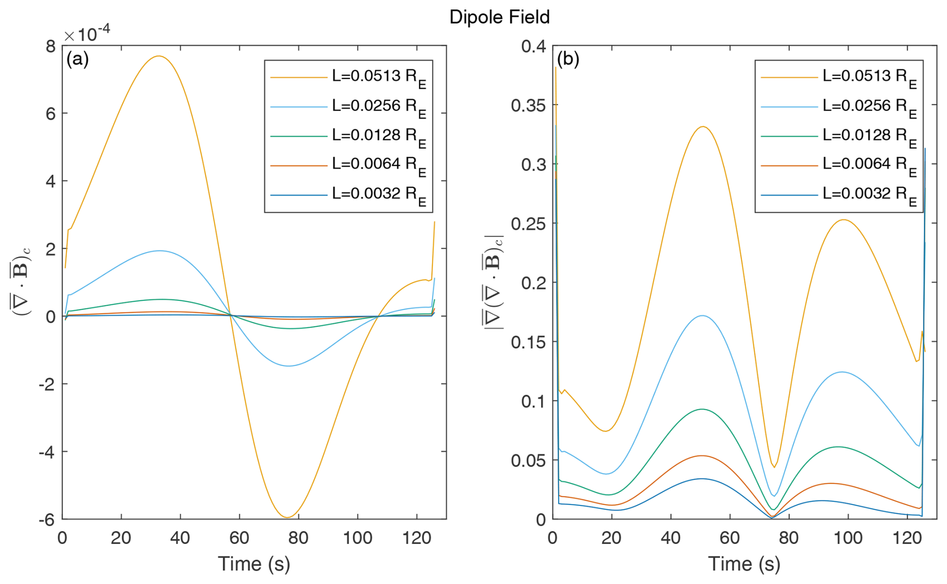
Figure 13 Dimensionless divergence and gradient of divergence for the magnetic field along the dipole-field crossing path with different characteristic S/C sizes (L).

The algorithm gradients were utilized to calculate the dimensionless divergence and the gradient of divergence for the magnetic field at the barycenter along the crossing path with different characteristic S/C sizes, with the results for the flux-rope and dipole-field cases shown in Figs. 12 and 13, respectively. Figures 12a and 13a show that the dimensionless divergence ${\left(\stackrel{\mathrm{‾}}{\mathbf{\nabla }}\cdot \stackrel{\mathrm{‾}}{\mathit{B}}\right)}_c$ at the barycenter is on the order of 10⁻⁴, while L varies from 0.0032 to 0.0513 R_E. The dimensionless gradient of the divergence $\left|\stackrel{\mathrm{‾}}{\mathbf{\nabla }}{\left(\stackrel{\mathrm{‾}}{\mathbf{\nabla }}\cdot \stackrel{\mathrm{‾}}{\mathit{B}}\right)}_c\right|$ for the flux-rope case was lower than 0.02 with L=0.0513 R_E, as shown in Fig. 12b. Similarly, Fig. 13b shows that $\left|\stackrel{\mathrm{‾}}{\mathbf{\nabla }}{\left(\stackrel{\mathrm{‾}}{\mathbf{\nabla }}\cdot \stackrel{\mathrm{‾}}{\mathit{B}}\right)}_c\right|$ was lower than 0.4, with L=0.0513 R_E, for the dipole field. Meanwhile, $\left|\stackrel{\mathrm{‾}}{\mathbf{\nabla }}{\left(\stackrel{\mathrm{‾}}{\mathbf{\nabla }}\cdot \stackrel{\mathrm{‾}}{\mathit{B}}\right)}_c\right|$ decreased with decreasing L in both cases. These results confirm the accuracy of the proposed method. As evidenced in Figs. 12 and 13, the errors in the first derivative decrease quadratically with the scale L, whereas the errors in the second derivatives decrease linearly with L.

5 Conclusions

In this study, a new algorithm was derived to estimate the linear and quadratic spatial gradients of the magnetic field from simultaneous seven- or nine-point magnetic measurements to obtain the fine structure of the magnetic field and the magnetic field geometry, allowing for the elucidation of whether the seven-spacecraft Plasma Observatory and the nine-spacecraft HelioSwarm missions could be utilized for such measurements. By inputting simultaneous seven–nine-point magnetic measurements and using the reference frame transformation relationships of the magnetic field as well as the least-squares method, the new algorithm performs several iterations to finally derive the convergent magnetic linear and quadratic spatial gradients.

The developed algorithm requires only one restriction on the spatial configuration of the constellations, which is that the constellations must be nonplanar. Actual operating constellations can easily satisfy this constraint. Only simultaneous magnetic measurements are required, with no other physical measurements needed, and the only physical constraint of the algorithm is the reference frame transformation relationship of the magnetic field. In this study, simultaneous magnetic measurements from seven or nine points were assumed to be obtained by identical instruments on board the space mission. Nowadays, the sampling time resolutions of the detectors are already very high, and the temporal variations in the magnetic field or magnetic spatial gradients can be obtained from the time series data. So, this algorithm only focuses on the magnetic spatial gradients, and the magnetic measurements from different spacecraft should be simultaneous. However, the real temporal measurements at different detectors may not be perfectly simultaneous, so the magnetic field data from different detectors need to be synchronized using interpolations. Furthermore, a homogeneous set of instruments on board the constellation may not be achieved, so systematic errors may arise. The total systematic error can be analyzed by the well-established error theory. In this study, the total truncation error has been evaluated. Furthermore, the iteration error, discretization error, and measurement error have been initially evaluated in the Appendix. It is found that the iteration error and discretization error are rather small for the dipole-field case and that the measurement error would cause large error, so the observation data should be filtered during the actual investigations as done in previous research (Shen et al., 2021a). Divergence-free magnetic field conditions were not required to calculate the magnetic spatial gradient. Alternatively, in the algorithm, the magnitudes of the magnetic divergence and its gradient were used to evaluate the truncation errors in the linear and quadratic magnetic spatial gradients, respectively.

The proposed algorithm was verified using a cylindrical force-free flux rope and a dipole magnetic field, with results showing that the iterations effectively converged and that the magnetic spatial gradients can reach reasonable accuracy. The results of this study can thus be applied to the analysis of magnetic field data from multi-spacecraft constellations (e.g., the Plasma Observatory and HelioSwarm) and to the design of future constellation missions.

Appendix A: Truncation error

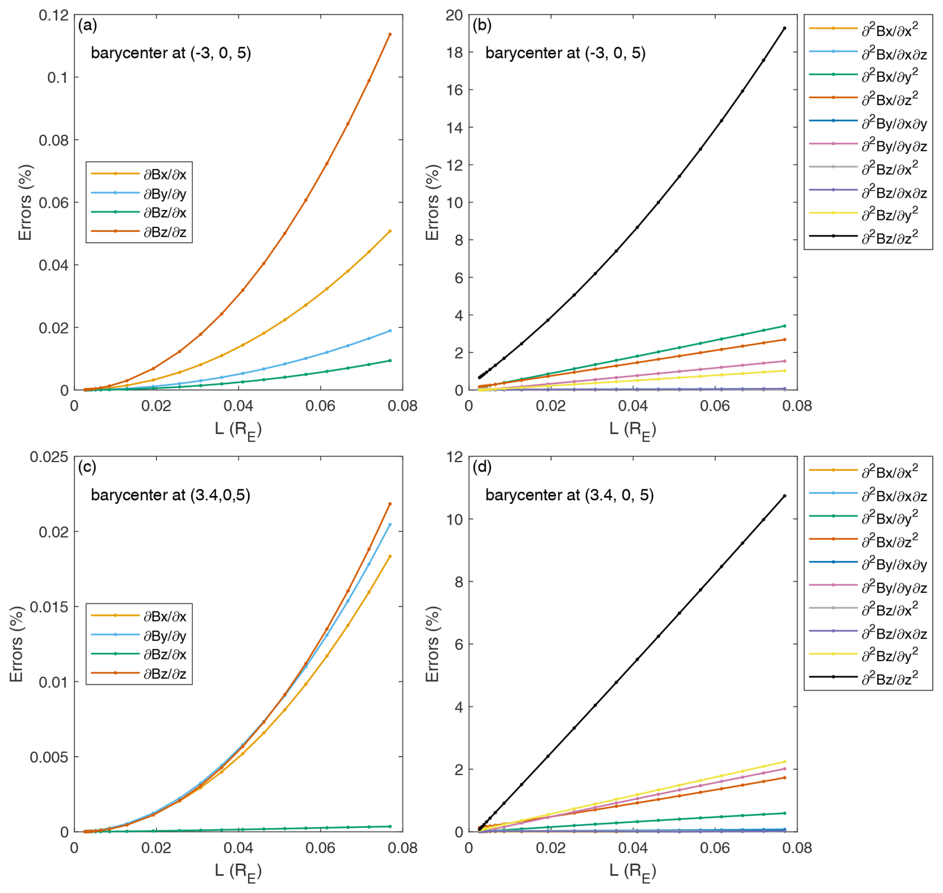
Figure A1 The total relative errors in the nonzero components of the linear and quadratic gradients with different characteristic size (L) at various barycenter positions for the dipole-field case.

In the following error analysis, only the dipole-field case is taken as an example. In Sect. 4, the dimensionless divergence and gradient of the divergence of the magnetic field have been used as the measures of the errors in the first-order and second-order magnetic gradients, respectively. And Fig. 13 shows the dimensionless divergence and gradient of the divergence with various characteristic S/C sizes. Nevertheless, the divergence and gradient of the divergence do not contain all the components of the magnetic gradients. In Appendix A, the truncation errors in the nonzero and independent components of the first-order and second-order magnetic gradients have been investigated, respectively. The truncation error is evaluated by the total relative error, which has been defined as $\left|\left(X_{\mathrm{algorithm}}-X_{\mathrm{accurate}}\right)/X_{\mathrm{accurate}}\right|\times \mathrm{100}$ % in Sect. 3.1. Figure A1 shows the total relative errors in the nonzero components of the linear and quadratic gradients with a different characteristic size (L). As evidenced in Fig. A1, the truncation error decreases as the distance between satellites is reduced. Furthermore, the errors in the first derivative decrease quadratically as the scale L is reduced, whereas the errors in the second derivatives decrease linearly with L reducing.

Appendix B: Iteration error

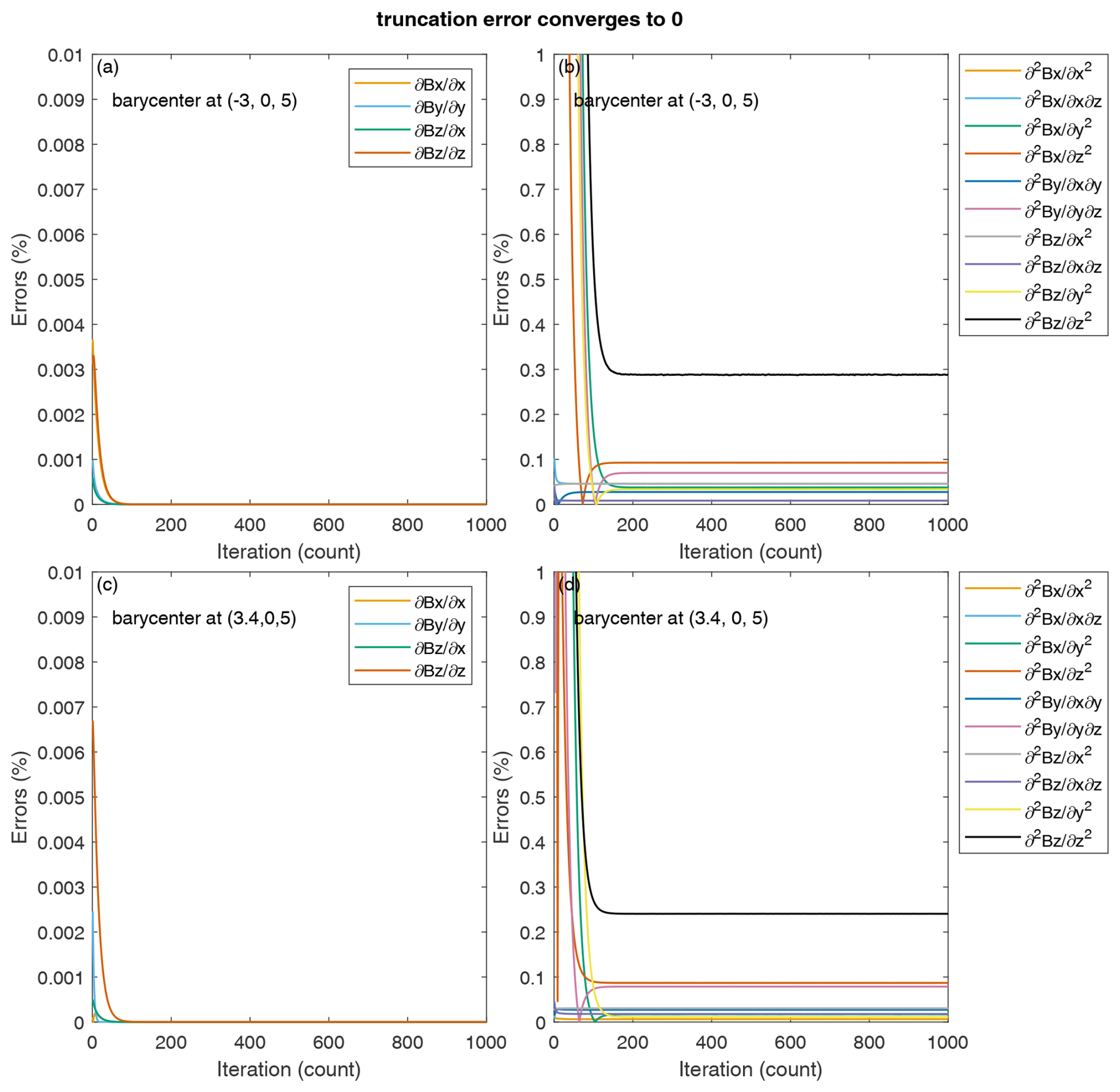
Figure B1 As the truncation error converges to zero, these are the total relative errors in the nonzero components of the linear and quadratic gradients with different iteration numbers at various barycenters for the dipole-field case.

By holding the configuration of the 7S/C constellation, the distances between satellites are scaled down by a factor of 100, which decreases the characteristic size of the 7S/C array to $L=\mathrm{0.2564}\times {\mathrm{10}}^{-\mathrm{3}}$ R_E. Due to this reduction, the high-order truncation error converges to zero. In Sect. 3.2, the cut-off number of iterations was set to 100. In order to clearly show the convergence of the iterations, the number of iterations was increased to 1000. Figure B1 shows the variation in the total relative errors in the linear and quadratic gradients with respect to the iteration numbers for the dipole-field case. The total relative errors in the four nonzero components of linear gradients at point (−3, 0, 5) and (3.4, 0, 5) are both lower than 10⁻⁶ %. The total relative errors in the 10 nonzero components of quadratic gradients at point (−3, 0, 5) are 0.0085 %, 0.0459 %, 0.0377 %, 0.0928 %, 0.0276 %, 0.0701 %, 0.0459 %, 0.0083 %, 0.0338 %, and 0.2880 %, while those at point (3.4, 0, 5) are 0.0063 %, 0.0304 %, 0.0171 %, 0.0870 %, 0.0271 %, 0.0788 %, 0.0304 %, 0.0180 %, 0.0112 %, and 0.2405 %, respectively. It is found that the total relative errors in the linear gradients decrease to 0 and those of the majority quadratic gradients decrease to less than 0.1 %, with the distances between satellites reduced. The iteration error goes to zero asymptotically.

Appendix C: Discretization error

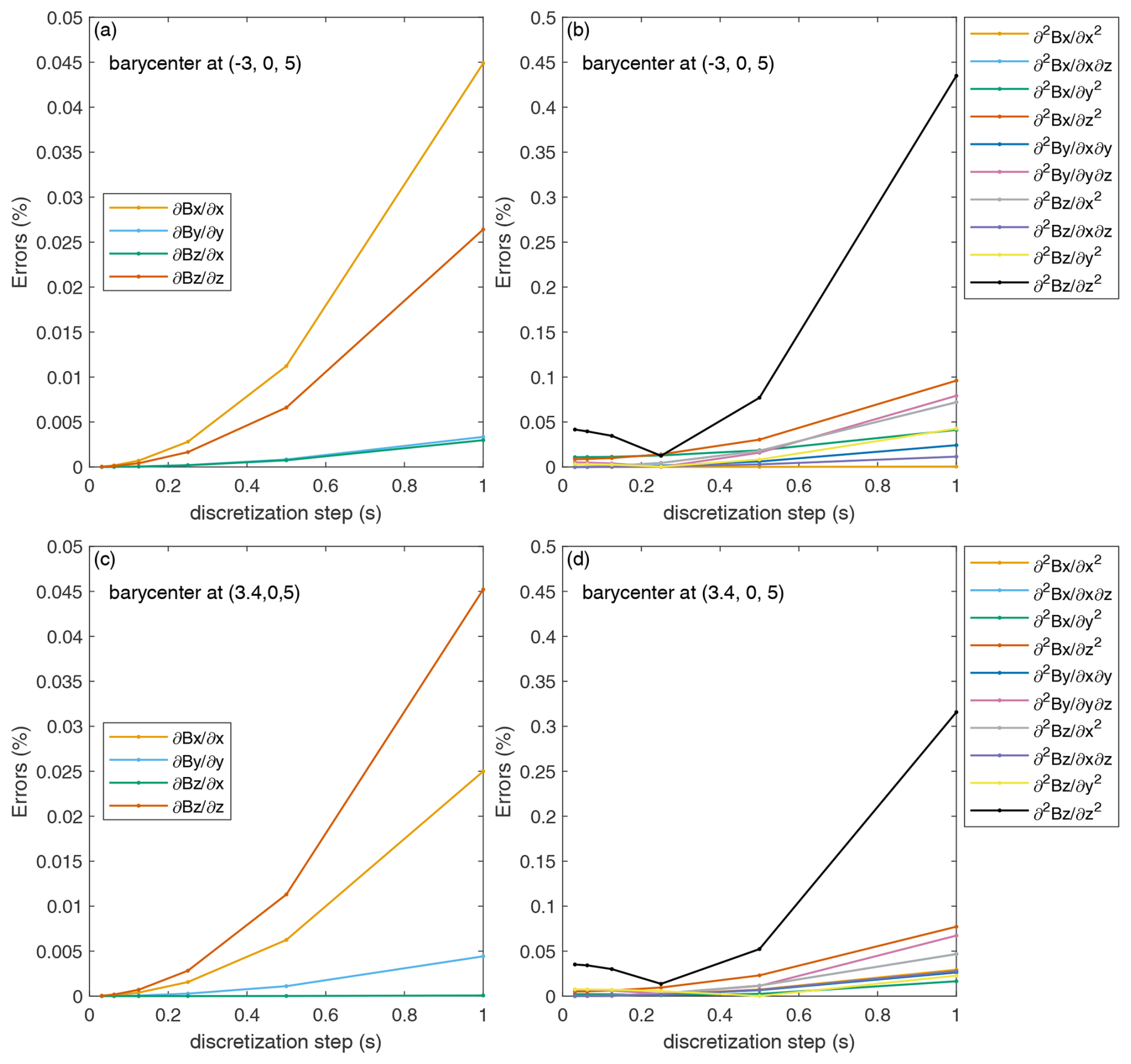
Figure C1 As the truncation error converges to zero, these are the total relative errors in the linear and quadratic gradients with different discretization steps at various barycenters for the dipole-field case, with a discretization error introduced.

In Sect. 3, the magnetic field measurement is instantaneous, and the resolution of measurement is set to 1 s. It is assumed that the magnetic field value at the measurement point is the average along the satellite's trajectory for a duration of 0.5 s before and after the point in the direction of the satellite's motion. This assumption introduces a discretization error, and the discretization step is defined as 1 s accordingly. The characteristic size of the 7S/C array is decreased to $L=\mathrm{0.2564}\times {\mathrm{10}}^{-\mathrm{3}}$ R_E. So, the truncation error converges to zero, leaving only the discretization error. If the resolution of the magnetic field measurement changes to 0.5 s, the duration time before and after the measurement point is set to 0.25 s accordingly. And the discretization step is reduced to 0.5 s. Figure C1 shows the variation in total relative errors in the linear and quadratic gradients with respect to the discretization steps for the dipole-field case, with a discretization error introduced. The total relative errors in the 4 nonzero components of linear gradients are no higher than 0.05 %, while the total relative errors in the 10 nonzero components of quadratic gradients are no higher than 0.5 %. The truncation error is decreased as the discretization step is reduced. It can be suggested that the discretization error is relatively small.

Appendix D: Measurement error

In order to evaluate the measurement error, the random Gaussian errors with a mean of 0 and a standard deviation of 0.01 are imposed on the magnetic field measurements. The results show that the total relative errors in linear gradients are about 1 %. However, the total relative errors in the majority of quadratic gradients are higher than 10 %, and individual errors even exceed 100 %. This algorithm would represent negative robustness to measurement noise. Shen et al. (2021a) have developed a novel algorithm that can estimate the quadratic magnetic gradient from multi-spacecraft measurements. This novel algorithm has been verified to be effective in analyzing MMS (Magnetospheric Multiscale mission) observations. In their investigation, the magnetic field data have to be filtered by a low-pass filter to eliminate disturbances; otherwise, the errors caused by these disturbances would be very large. It can be suggested that the observation data should be filtered to remove noise when applying our algorithm.