Deep temporal convolutional networks for F_10.7 radiation flux short-term forecasting

F_10.7, the solar flux at a wavelength of 10.7 cm (F_10.7), is often used as an important parameter input in various space weather models and is also a key parameter for measuring the strength of solar activity levels. Therefore, it is valuable to study and forecast F_10.7. In this paper, the temporal convolutional network (TCN) approach in deep learning is used to predict the daily value of F_10.7. The F_10.7 series from 1957 to 2019 are used. The data during 1957–1995 are adopted as the training dataset, the data during 1996–2008 (solar cycle 23) are adopted as the validation dataset, and the data during 2009–2019 (solar cycle 24) are adopted as the test dataset. The leave-one-out method is used to group the dataset for multiple validations. The prediction results for 1–3 d ahead during solar cycle 24 have a high correlation coefficient (R) of 0.98 and a root mean square error (RMSE) of only 5.04–5.18 sfu. The overall accuracy of the TCN forecasts is better than the autoregressive (AR) model (it only takes past values of the F_10.7 index as inputs) and the results of the US Space Weather Prediction Center (SWPC) forecasts, especially for 2 and 3 d ahead. In addition, the TCN model is slightly better than other neural network models like the backpropagation (BP) neural network and long short-term memory (LSTM) network in terms of the solar radiation flux F_10.7 forecast. The TCN model predicted F_10.7 with a lower root mean square error, a higher correlation coefficient, and a better overall model prediction.

1 Introduction

Solar activity has a significant impact on the Earth's climate, electromagnetic fields, and communication systems, among other things. F_10.7 (2800 MHz, 10.7 cm solar flux) is a typical parameter for characterizing solar activity levels, representing the cyclical variability of solar activity (Tapping, 2013). The F_10.7 index is an important parameter for predicting atmospheric density for spacecraft orbits and ionospheric forecasts affecting communication. For example, F_10.7 is used as a control parameter in ionospheric models to calculate the variation of radio signal properties (Ortikov et al., 2003). F_10.7 is also widely used for satellite, navigation, communication, and terrestrial climate (Huang et al., 2009; Yaya et al., 2017). Therefore, accurate forecasting of F_10.7 is not only of great value for the conduct of application but is also of comparative importance in the scientific study of space weather forecasting (Katsavrias et al., 2021; Simms et al., 2023).

F_10.7 has a clear periodicity, e.g., 27 d, 11 years. But the cycles are not simply repetitive but have similar but different fluctuations, so the core of the F_10.7 prediction problem for time series data is to uncover the potential patterns of historical data and predict the future data as far as possible (Lampropoulos et al., 2016). The F_10.7 index forecast model is based on a time series model. Many researchers have used different methods to build predictive models for F_10.7. Mordvinov (1986) used a multiplicative autoregressive model to forecast the monthly mean F_10.7, but the model had a large error in predicting it. Warren et al. (2017) built optimized independent models for each forecast date, and the results showed that this approach typically had better prediction skill than autoregressive methods. Zhong et al. (2010) utilized the singular-spectrum analysis signal processing technique to predict the F_10.7 index of solar activity for the next 27 d. The research result indicated that the method performed well in predicting the periodic variations of the F_10.7 index. Henney et al. (2012) predicted F_10.7 using the global solar magnetic field generated by the energy transport model, with a Pearson correlation coefficient of 0.97 for 1 d ahead. Liu et al. (2018) applied two models by Yeates et al. (2007) and Worden and Harvey (2000) to predict short-term variability in F_10.7 . During low levels of solar activity, the predicted values of the model were closer to the observed values.

With the rapid development of machine learning and neural networks, researchers are increasingly intrigued by the powerful learning capabilities of machine learning and neural networks, using them to study variations in solar activity. The support vector machine regression method was used by Huang et al. (2009) to predict daily values of solar activity F_10.7. Xiao et al. (2017) used the backpropagation (BP) neural network to forecast the daily-mean F_10.7 index of solar activity for short-term prediction. The results showed that using BP neural networks to predict the solar activity daily F_10.7 index was superior to the results of Huang et al. (2009). Luo et al. (2020) proposed a method for predicting the 10.7 cm radio flux in multiple steps. The method is a combination of the empirical mode decomposition (EMD) and BP neural network to construct an EMD–BP model for predicting F_10.7 values. The method significantly reduces the prediction error for high levels of solar activity compared to support vector machine regression (SVR) and the BP neural network. Zhang et al. (2022) proposed a short-term forecast of the solar activity daily-mean F_10.7 index using a long short-term memory (LSTM) network method. The forecast had a high correlation coefficient (R) of 0.98 and a low root mean square error (RMSE) range of 6.20–6.35 sfu. Although the above recurrent neural network (RNN)-based architecture and its variants achieved a good prediction accuracy of F_10.7, the training process of a model often spends a significant amount of time and computational memory and also frequently encounters issues such as gradient explosion or vanishing gradients during network training (Lipton et al., 2015; Yang et al., 2021). To this end, Bai et al. (2018) proposed a neural network called the temporal convolutional network (TCN), in which long input sequences can be processed as a whole in the TCN. TCNs use convolutional operations for efficient parallel computation. In addition, the backpropagation path of TCNs is different from the time direction of the sequence, which makes TCNs avoid the gradient problem in RNN. Given the above advantages and for the variability characteristics of F_10.7 time series data, this paper introduces machine-learning-based TCN-related theories and techniques into the forecasting of F_10.7 and compares the results of TCN prediction with other classical models to verify their effectiveness and feasibility in short-term forecasting.

2 Data and method

2.1 Data source and data processing

F_10.7 represents the solar radiation flux at a wavelength of 10.7 cm, and the magnitude of this index describes the intensity of solar activity. The 10.7 cm solar flux is given in solar flux units (1 sfu = 10⁻²² W m⁻² Hz⁻¹). The 10.7 cm daily solar flux data were obtained from the website of the National Oceanic and Atmospheric Administration. Three flux determinations are done each day. Each 10.7 cm solar flux measurement is expressed in three values: the observed, adjusted, and URSI Series D values (absolute values). The observed value is the number measured by the solar radio telescope. This is modulated by two quantities: the level of solar activity and the changing distance between the Earth and Sun. Since it is a measure of the emissions due to solar activity hitting the Earth, this is the quantity to use when terrestrial phenomena are being studied (Tapping, 1987). When studying the Sun, it is undesirable to have the annual modulation of the 10.7 cm solar flux caused by the changing distance between the Earth and Sun. However, during the ephemeris calculations required for the solar flux monitors to accurately acquire and track the Sun, one of the byproducts obtained is the distance between the Sun and the Earth. Therefore, we generate an additional value called the adjusted value, which takes into account the variations in the Earth–Sun distance and represents the average distance. Absolute measurements of flux density are quite difficult. Astronomers attempt to match the solar flux density data at various frequencies with a frequency spectrum by applying a scale factor. By combining each wavelength with the calibrated spectrum, a series of D flux is obtained, where D flux equals 0.9 multiplied by the adjusted flux (Tanaka et al., 1973).

Between March and October measurements are made at 17:00, 20:00 (local noon), and 23:00 UT. However, the combination of location in a mountain valley and a relatively high latitude makes it impossible to maintain these times during the rest of the year. Consequently, from November to February, the flux determination times are changed at 18:00, 20:00, and 22:00, so that the Sun is high enough above the horizon for a good measurement to be made. Therefore, we chose the adjusted flux value of F_10.7 measured at 20:00 UT (local noon). The data during 1957–1995 are adopted as the training dataset, the data during 1996–2008 (solar cycle 23) are adopted as the validation set, and the data during 2009–2019 (solar cycle 24) are adopted as the test set. Figure 1 shows the data. The black line represents the training dataset, the red line represents the validation dataset and the blue line is the testing dataset.

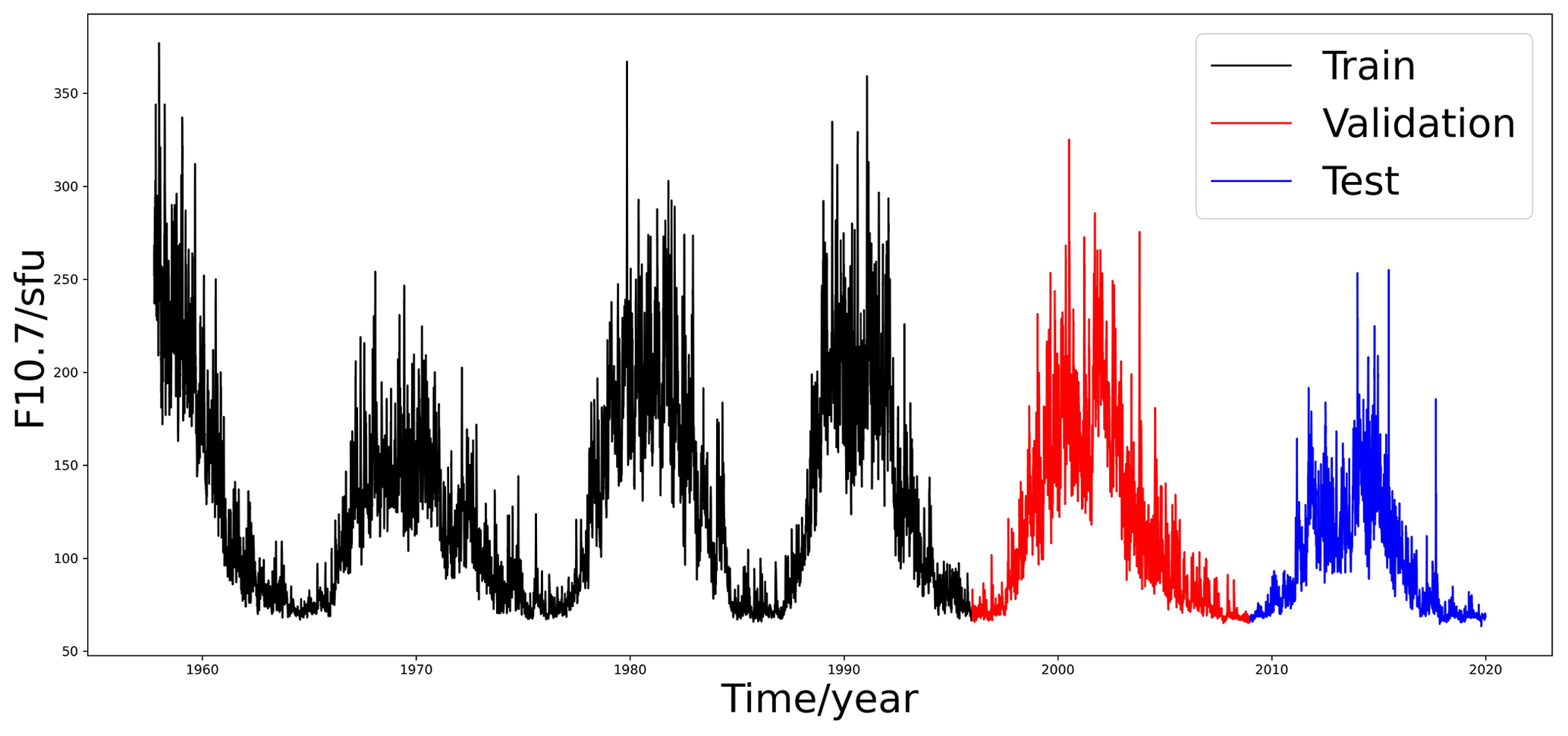
Figure 1 The daily values of the F_10.7 index from 1957 to 2019. The black line represents the training set (solar cycles 19–22), red represents the validation set (solar cycle 23), and blue represents the test set (solar cycle 24).

In this paper, the hardware environment used for the solar radiation flux F_10.7 experiment is NVIDIA^® GeForce 940MX, CPU is Inter^® Core™ i5-6200. We build a model using Python and utilize some efficient frameworks including Pandas, Matplotlib, TensorFlow, and Sklearn. Pandas is a powerful data analysis library that provides several methods for processing and analyzing the parameters of the solar flux F_10.7, such as selective sorting, merging, and aggregating. Matplotlib is a plotting Python library that provides a rich set of customization options for this paper to visualize the predicted results of the solar flux F_10.7 as well as to analyze the related results. Sklearn is an open-source, third-party library for machine learning model training and big data mining that provides a unified interface for many machine learning algorithms and a number of tools for evaluating model performance and tuning hyperparameters. TensorFlow is also an open-source machine learning library for building, training, and deploying a variety of model types, including regression, classification, and convolutional neural network and recurrent neural network construction. In this paper, the network construction, training, parameter tuning, and evaluation of the prediction model for solar radiation flux F_10.7 are based on the above two machine learning libraries.

2.2 Method

The TCN was proposed by Bai et al. (2018). Some scholars have demonstrated that the TCN not only achieves better performance but also reduces the computational cost for training, compared to that of RNN (Lea et al., 2017; Bai et al., 2018; Dieleman et al., 2018). The TCN combines both RNN and convolutional neural network (CNN) architectures and is a convolutional neural network variant designed to handle time series modeling problems. The TCN is well adapted to the temporal nature of the data using both causal and extended convolutional structures to extract feature information. The convolutions in the TCN are causal, meaning there is no information leakage from future time steps. This distinguishes the TCN from other recurrent neural networks such as LSTM and GRU (gated recurrent unit) networks, which require gate mechanisms. As a result, the TCN achieves higher accuracy and longer memory without the need for gate mechanisms. Long input sequences can be processed as a whole in the TCN. The TCN does not have the advantages of gradient disappearance and gradient explosion problems. Here, the TCN is introduced to model the prediction of F_10.7.

For the prediction of a univariate time series, the TCN model takes lagged observations of the time series as inputs and predicts future F_10.7 sequence values as outputs. Each set of input patterns consists of moving a fixed-length window in the time series. The principle of forecasting is represented in Fig. 2. The original F_10.7 data are lengthy, and during training, a continuous subsequence needs to be inputted. The output and input lengths of the temporal convolutional network (TCN) are equal, meaning the length of the output sequence generated by the TCN is equal to the specified input length. To meet the prediction requirements, the specific number of steps to forecast (referred to as output length) should not exceed input length, allowing for partial overlap between the input and output sequences.

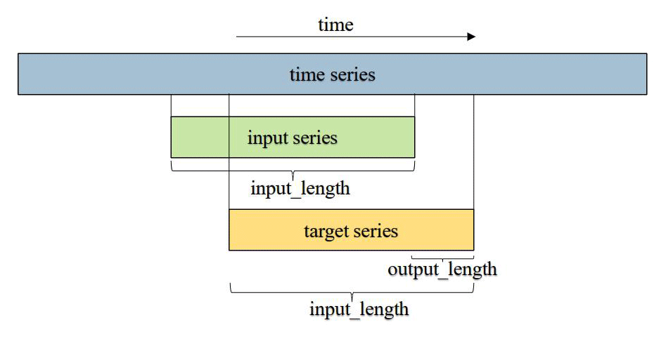
Figure 2 Diagram of F_10.7 sequence data prediction. The blue part represents the original sequence, the green part represents the input subsequence, and the orange part represents the overlap and the actual predicted lengths.

Supposed the input of F_10.7 is $x=(x_{\mathrm{0}},x_{\mathrm{1}},\mathrm{\dots },x_T)$, the desired output sequence is $y=(y_{\mathrm{0}},y_{\mathrm{1}},\mathrm{\dots },y_T)$, where the two sequences x,y satisfy the causal relationship. The input $x_{\mathrm{0}},x_{\mathrm{1}},\mathrm{\dots },x_{t-\mathrm{1}}$ observed at the previous moment be used to predict the output y_t at moment t. The modeling objective of the TCN is to generate any hidden function mapping, which means that the prediction of the F_10.7 sequence can be represented as

$$\begin{array}{}\text{(1)}& {\widehat{y}}_{\mathrm{1}},\mathrm{\dots },{\widehat{y}}_{T+\mathrm{1}}=f(x_{\mathrm{0}},x_{\mathrm{1}},\mathrm{\dots },x_i,\mathrm{\dots },x_T),\end{array}$$

where x_i and ${\widehat{y}}_i$ are the observed and predicted values of F_10.7 at time i, respectively, and f is the mapping of the function trained by the TCN.

The TCN is one of the algorithms developed on the basis of the convolutional neural network (CNN). The CNN uses a one-dimensional convolutional network, consisting of an inflated causal convolution and a residual module.

One-dimensional convolution operates on time series and extracts various features, but as the length of the time series grows, a regular convolutional network requires more convolutional layers to receive longer sequences. Extended convolution, on the other hand, improves on convolution by allowing interval sampling of the input for convolution with a number of layers L and a convolution kernel of size k with an acceptance domain of

$$\begin{array}{}\text{(2)}& r={\mathrm{2}}^{(L-l)}k.\end{array}$$

The causal extended convolution operation F for element s in a time series is defined as

$$\begin{array}{}\text{(3)}& F\left(s\right)=(x\ast \mathit{f})\left(s\right)=\sum _{i=\mathrm{0}}^{k-\mathrm{1}}\mathit{f}\left(i\right)\cdot x_{s-d\cdot i},\end{array}$$

where $x=(x_{\mathrm{0}},x_{\mathrm{1}},\mathrm{\dots },x_T)$ is the input vector, d is the expansion factor, ∗ is the causal expansion convolution operator, f is the convolution kernel vector, k is the convolution kernel size, and $s-d\cdot i$ indicates the past direction of the input.

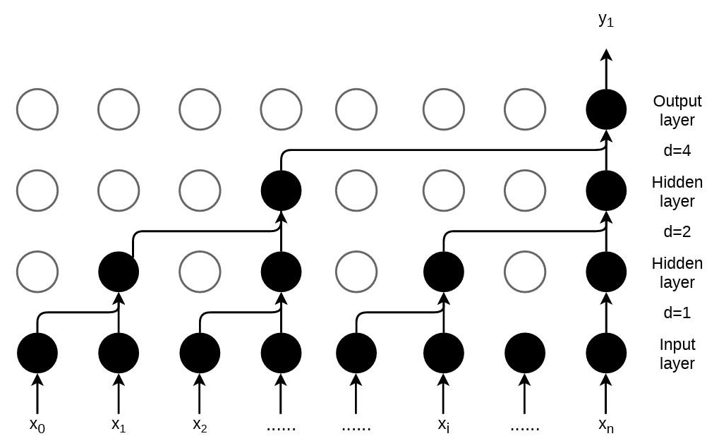
The expanding causal convolution for a convolution kernel size k of 3 is illustrated in Fig. 3, where the output y₁ at moment t is determined by the current input as well as the previous inputs; i.e., $x_{\mathrm{0}},x_{\mathrm{1}},\mathrm{\dots },x_n$. This shows that the predicted output is not affected by future information and therefore avoids information leakage. In addition, the introduction of the expansion factor d to the input of the convolutional layer matrix is sampled at intervals. In the first hidden layer, the sampling interval rate d=1, which represents each point of the input, is sampled. In the second hidden layer, the sampling interval rate d=2; i.e., every two points are taken, ignoring one neuron. At higher layers, d grows exponentially, thus allowing for fewer layers to achieve a larger receptive field with fewer layers. The expanding causal convolution can be adjusted by varying the number of layers, perceptual field size, convolution kernel size, and expansion coefficient. This helps to address the challenge in CNNs where the length of temporal modeling is limited by the size of the convolution kernel. Compared to traditional neural networks like LSTM and BP, the TCN overcomes issues such as gradient vanishing and exploding. At the same time, the TCN possesses advantages such as lower memory consumption, stable gradient, improved parallelism, and flexible perceptual field.

Figure 3 Expansion causal convolutional structure diagram.

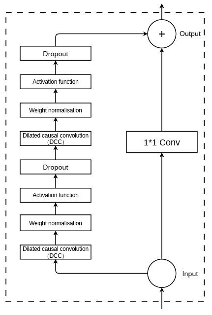
The structure of the residual module in the TCN is shown in Fig. 4. ReLU (rectified linear unit) is used as an activation function. To avoid the problem of gradient explosion, the weight normalization layer is added. To avoid overfitting, a dropout layer is added for regularization. The residual links allow the network to pass information across layers, thus avoiding information loss due to too many layers. Residual convolution is introduced for layer hopping, and 1 × 1 convolution is performed to ensure that the input and output remain consistent.

Figure 4 Expansion causal convolutional structure diagram.

2.3 Selection of training parameters

A key component of the machine learning model training process is called the loss function, which gives direction to the optimization of the model by measuring the difference between the model output $\widehat{y}$ and the observation y. The smaller the loss function, the better the robustness of the model. The L1 norm loss function is extensively utilized in deep learning tasks (Zhao et al., 2017). It possesses a notable advantage of being insensitive to outliers and exceptional values, consequently avoiding the gradient explosion issue. Moreover, the loss function provides a more robust solution by offering stability. Therefore, the L1 loss function is chosen to construct the loss function for the predicted and observed values of the F_10.7 sequence. The function is defined as

$$\begin{array}{}\text{(4)}& L(\widehat{y},y)=\sum _{i=\mathrm{0}}^n\mathrm{|}{\widehat{y}}_i-y_i\mathrm{|},\end{array}$$

where ${\widehat{y}}_i$ is the predicted value of F_10.7 at moment i, and y_i is the observed value of F_10.7 at moment i.

To build the TCN model that is not merely a linear regression model, it is essential to introduce nonlinearity by adding a ReLU activation function at the top of the convolutional layers. The function is defined as

$$\begin{array}{}\text{(5)}& f\left(x\right)=max(\mathrm{0},x),\end{array}$$

where $x=(x_{\mathrm{0}},x_{\mathrm{1}},\mathrm{\dots },x_T)$ is the input vector.

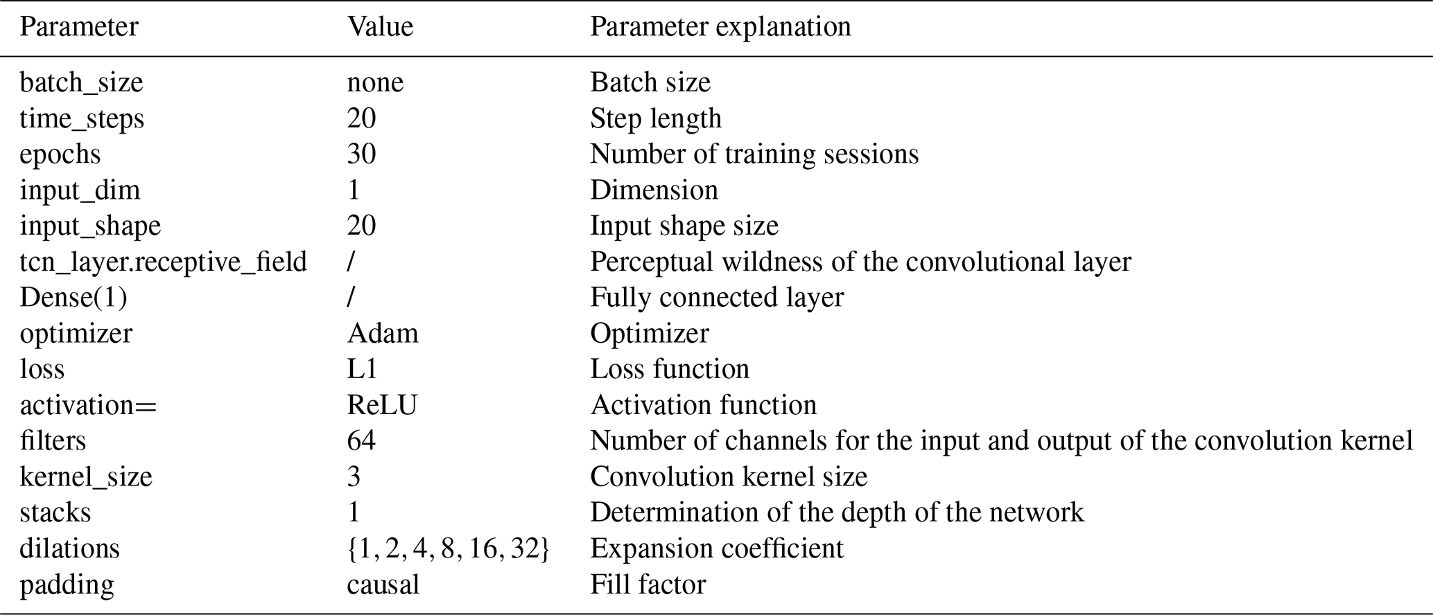
To counteract the problem of gradient explosion, weights are normalized at each convolutional layer. To prevent overfitting, each convolutional layer is followed by a dropout for regularization. After several training sessions, the optimal parameters for model training are shown in Table 1.

Table 1 Training parameters of the TCN model.

2.4 Forecast evaluation criteria

In order to quantify the forecast performance of the model, we chose five evaluation metrics. The chosen performance metrics include the mean absolute error (MAE), the mean absolute percentage error (MAPE), and the root mean square error (RMSE) for accuracy; the correlation coefficient (R) for association; and the error (σ) for bias. Five commonly used model evaluation metrics were employed to assess predictive performance (Liemohn et al., 2021).

$$\begin{array}{}\text{(6)}& {\displaystyle }\mathrm{MAE}={\displaystyle \frac{\mathrm{1}}{\mathrm{N}}}\sum _{i=\mathrm{1}}^N\mid f_i-F_i\mid \text{(7)}& {\displaystyle }\mathrm{RMSE}=\sqrt{{\displaystyle \frac{\mathrm{1}}{N}}\sum _{i=\mathrm{1}}^N(f_i-F_i{)}^{\mathrm{2}}}\text{(8)}& {\displaystyle }\mathrm{MAPE}={\displaystyle \frac{\mathrm{1}}{N}}{\displaystyle \frac{\sum _{i=\mathrm{1}}^N\mid f_i-F_i\mid }{f_i}}\text{(9)}& {\displaystyle }R={\displaystyle \frac{\sum _{i=\mathrm{1}}^N(f_i-\stackrel{\mathrm{‾}}{f})(F_i-\stackrel{\mathrm{‾}}{F})}{\sqrt{\sum _{i=\mathrm{1}}^N(f_i-\stackrel{\mathrm{‾}}{f}{)}^{\mathrm{2}}}\sqrt{\sum _{i=\mathrm{1}}^N(F_i-\stackrel{\mathrm{‾}}{F}{)}^{\mathrm{2}}}}}\text{(10)}& {\displaystyle }\mathit{\sigma }=f_i-F_i,\end{array}$$

where MAE denotes the mean absolute error, MAPE denotes the mean absolute percentage error, RMSE denotes the root mean square error, R denotes the linear correlation coefficient, N denotes the number of samples, f_i denotes the forecast, F_i denotes the observation, $\stackrel{\mathrm{‾}}{f}$ is the mean of f_i, and $\stackrel{\mathrm{‾}}{F}$ is the average of F_i. Each indicator evaluates the model in a different perspective. Among them, MAE represents the average absolute error between predicted values and actual values. RMSE represents the root mean square error between predicted values and actual values. R represents the degree of trend fitting between predicted values and actual values. σ represents the error between predicted values and actual values. Therefore, the smaller the MAE, MAPE, and RMSE and the larger the R, the better the model prediction.

3 Results and discussion

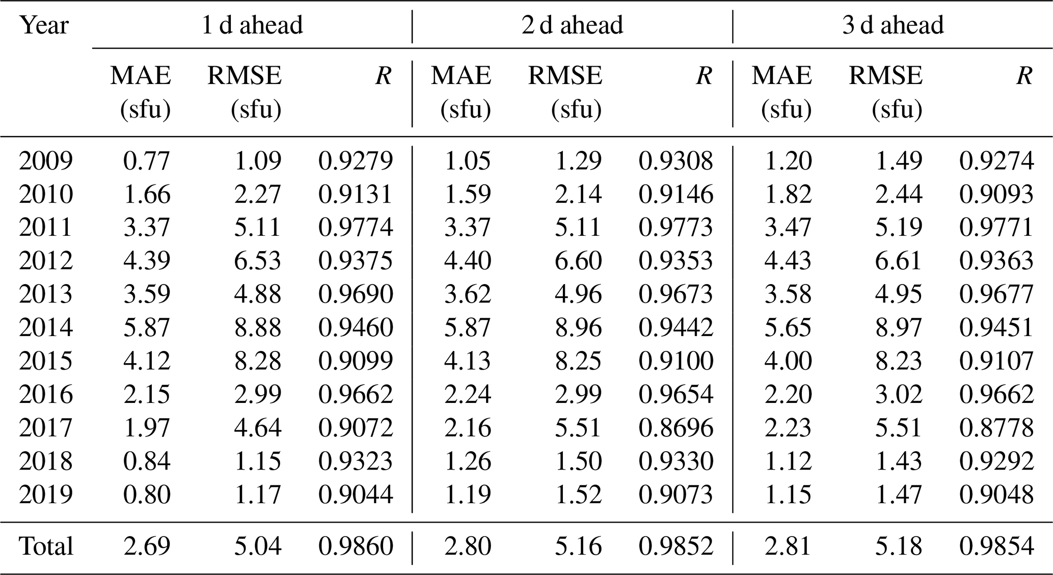
The TCN model is used to predict the values of F_10.7 for 1–3 d ahead. Table 2 shows the evaluation metrics of TCN model predictions compared to observations for different years of the 24 solar cycle. The table represents the performance of the TCN model in different years. In Table 2, it can be seen that the TCN model predicts F_10.7 with a root mean square error (RMSE) ranging from 1 to 9 sfu for 1 d ahead and an average absolute error (MAE) ranging from 0 to 6 sfu. The highest correlation coefficient reaches up to 0.98. For 2 and 3 d ahead, the RMSE ranges from 1 to 9 sfu, the MAE ranges from 1 to 6 sfu, and the highest correlation coefficient remains at 0.98. Irrespective of the lead time, be it 1, 2, or 3 d, the TCN model demonstrates consistent performance with relatively small ranges of root mean square error and mean absolute error, accompanied by a consistently high correlation coefficient. The results demonstrate the stability of the TCN model. However, the magnitude of prediction errors for 1–3 d ahead forecasts varies across different years. For example, the RMSE for a 1 d ahead forecast is 1.09 sfu in 2009, while its value is 8.88 sfu in 2014. Li et al. (2023) defined the years in which the mean value of F_10.7 is greater than 110 sfu as having high solar activity and the years in which the mean value is less than 110 sfu as having low solar activity. In this paper, the annual average of F_10.7 from 2011 to 2015 is greater than 110 sfu, so the years from 2011 to 2015 are called high-solar-activity years, and the remaining years are called low-solar-activity years. Table 2 shows that solar activity has a periodic effect, and the prediction accuracy of the model is negatively correlated with the intensity of solar activity. The magnitude of error is related to the year of high and low solar activity.

Table 2 The prediction errors (MAE, RMSE) and R of the TCN model for the F_10.7 data during 2009–2019.

To further validate the performance of the model, we use the leave-one-out method for cross-validation (Aminalragia et al., 2020). We leave iteratively one solar cycle out as a test dataset and rerun the model each time (e.g., keep solar cycle 23 as the test dataset and train the model with the remaining solar cycles and then keep solar cycle 22 as the test dataset and train the model with the remaining solar cycles). The results of the tests are shown in the Table 3. It can be seen that cycles with stronger solar activity are found to have larger model forecast errors. For cycles with weaker solar activity, the results are better. Solar cycles 20 and 24 have about the same intensity of solar activity and are both weaker. The model forecasts are better. Solar cycles 21 and 22 have about the same intensity of solar activity and are both stronger. The model forecasts are poorer. However, the overall average prediction results do not change much compared to solar cycle 24. The prediction accuracy of the model is negatively correlated with the intensity of solar activity. The results show that the change of prediction accuracy of the model is related to the intensity of solar activity. The F_10.7 data have a solar cycle effect. The TCN model does not largely affect the final F_10.7 forecasts due to specific properties of the data.

Table 3 The prediction errors (MAE and RMSE) and R of the TCN model for the F_10.7 data during different solar cycles.

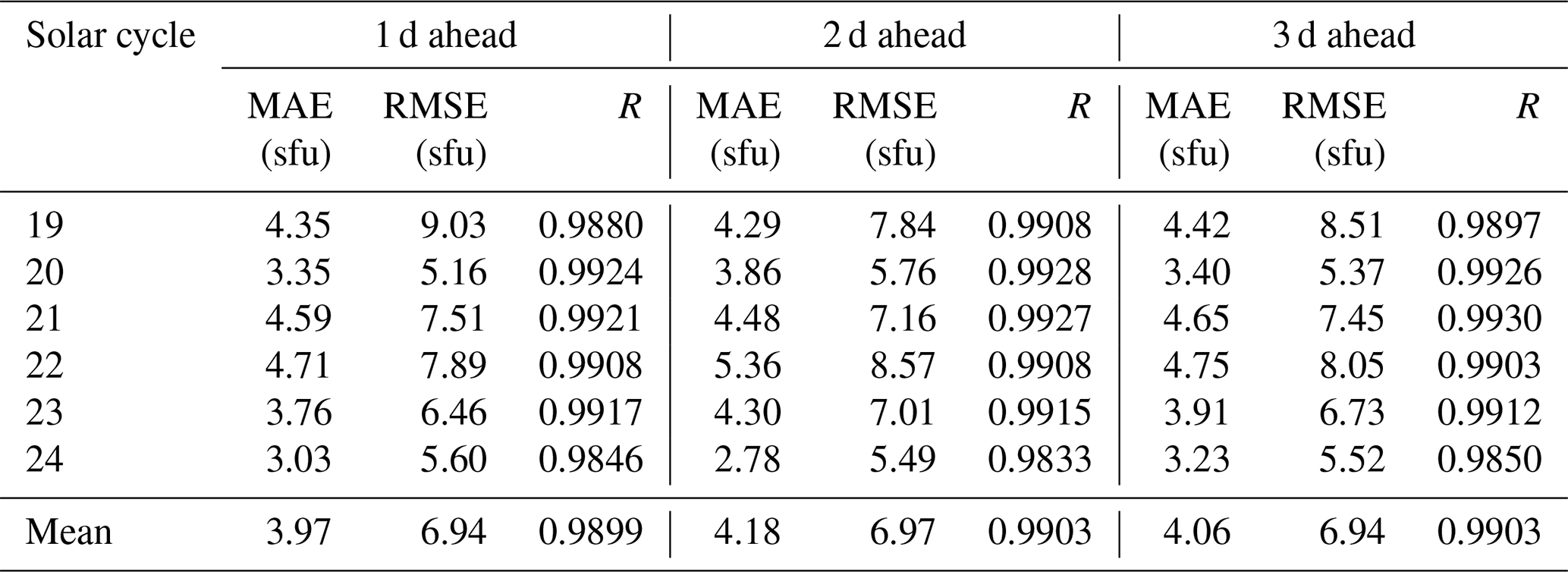
Figure 5 displays the frequency distribution of the difference between the observed value and the predicted value of the model. To maintain the compactness of the histogram, differences greater than 15 sfu and smaller than −15 sfu are not displayed. As can be seen from Fig. 5, the prediction differences for 2 d ahead are skewed towards the right. The differences in predictions for 3 d ahead are skewed towards the left. Despite these differences, frequency is maximized when the difference between the observed and predicted values is in the vicinity of zero, and most predictions (88.5 % of the 1–3 d ahead forecast) were located within ±6 sfu of error.

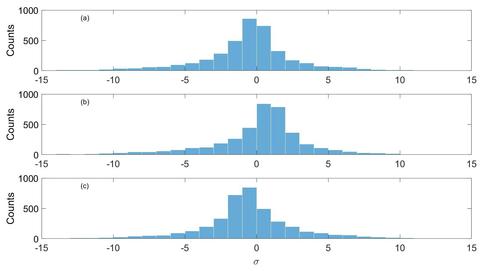
Figure 5 Frequency distribution of the difference between the observed values and the model predictions during 2009–2019 (solar cycle 24) for 1 d ahead (a), 2 d ahead (b), and 3 d ahead (c).

The high-solar-activity years of 2013–2014 and the low-solar-activity year of 2018 are chosen for comparison in solar cycle 24. We chose predicted values from 15 January to 15 February in 2013, 2014, and 2018 to compare with observed values and improve image representation. Figure 6 shows the predicted effects for high-solar-activity years in panels (a)–(b) and the low-solar-activity year in panel (c) in solar cycle 24. The black line represents observed values, while the blue dots represent predicted values. As can be seen from Fig. 6, it shows that the TCN model effectively predicts the trend of F_10.7 and exhibits good agreement in terms of magnitude between the observed and predicted values for the majority of the time. Especially during the peak of F_10.7, the TCN model's predictions align well with the actual values, and it performs exceptionally well during periods of high solar activity.

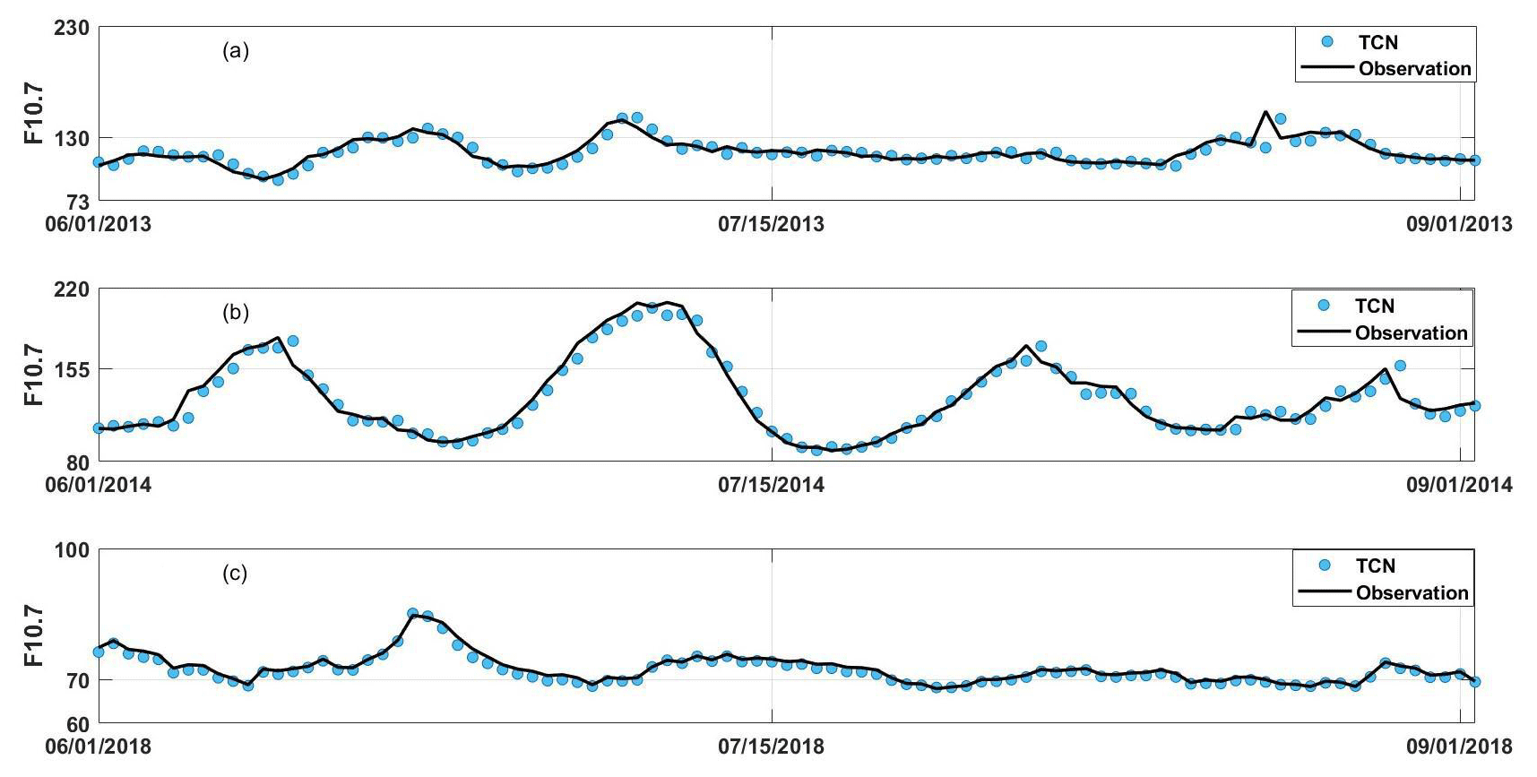
Figure 6 Predicted effects for high-solar-activity years in (a)–(b) and the low-solar-activity year in (c) for 1 d ahead in solar cycle 24. The black line represents observed values, while the blue dots represent predicted values

To assess the model's effectiveness, we compare the TCN model's forecasting results with those of the US Space Weather Prediction Center (SWPC) forecast (https://www.swpc.noaa.gov/sites/default/files/images/u30/F10.7 Solar Flux.pdf, last access: 9 April 2024) and the AR model (Du, 2020) for 1–3 d ahead. Furthermore, we compare the predictions with the BP model (Xiao et al., 2017) and LSTM (Zhang et al., 2022) for 3 d ahead.

Figure 7 shows the prediction results of the SWPC compared to the TCN model for 1 d ahead in panel (a), 2 d ahead in panel (b), and 3 d ahead in panel (c). The blue bars represent the predicted outcome parameters for the SWPC, and the yellow bars represent the predicted outcome parameters for the TCN model. Figure 7 shows that the TCN model's predictions are generally better than the forecasts of the SWPC. Compared with F_10.7 values for 1–3 d ahead, the TCN model's prediction for 1 d ahead is only 0.07 sfu higher than the SWPC forecast in 2012, while in other years, the TCN model consistently outperformed the SWPC forecast. Particularly for predictions 2 and 3 d ahead, the TCN model's performance is significantly better than the SWPC forecast. The RMSE of the TCN is 5.11 sfu for 1 d ahead, while the RMSE of the SWPC is 5.61 sfu in 2011. The RMSE of the TCN is 0.50 sfu lower than the SWPC, representing a relative decrease of 10 %. For prediction 2 d ahead, the RMSE of the TCN is 5.11 sfu, while the SWPC of RMSE is 9.17 sfu in 2012. The RMSE of the TCN is approximately 4.06 sfu lower than the SWPC, representing a relative decrease of 79 %. For prediction 3 d ahead in 2011, the RMSE of the TCN is 5.19 sfu, while the RMSE of the SWPC is 11.46 sfu. The RMSE of the TCN is approximately 6.27 sfu lower than the SWPC, representing a relative decrease of 120 %. All these results show that the TCN model proposed in this paper has a better performance relative to the SWPC model. The TCN model is feasible for F_10.7 prediction.

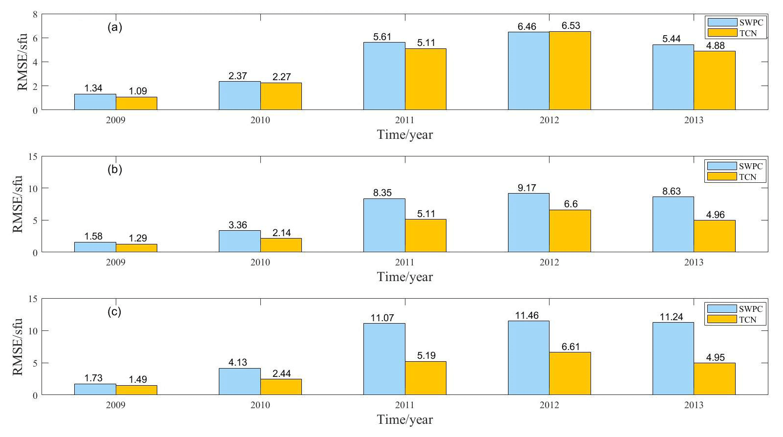
Figure 7 Comparison of the prediction performance of the SWPC and TCN for (a) 1 d ahead, (b) 2 d ahead, and (c) 3 d ahead during different years.

Figure 8 shows the prediction results of the AR model compared to the TCN model for 1 d ahead in panel (a), 2 d ahead in panel (b) and 3 d ahead in panel (c). The blue bars represent the predicted outcome parameters for the AR model, and the yellow bars represent those for the TCN model. As can be seen in Fig. 8, the TCN model outperforms the AR model overall in forecasting for 1–3 d ahead. The TCN model only has forecasts that are 0.96 and 0.04 sfu larger than the AR model pattern for 1 d ahead in 2014 and 2019, respectively. In addition, the TCN model outperforms the AR model in forecasting for both 2 and 3 d ahead. The RMSE of the TCN is only 5.19 sfu for predicting outcomes for 3 d ahead in 2011, while the RMSE of the AR model is 10.43 sfu. The stability and prediction accuracy of the TCN model in predicting F_10.7 are again verified.

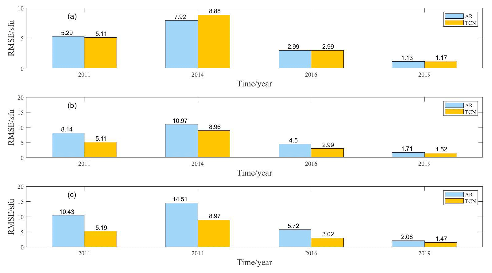
Figure 8 Comparison of the prediction performance of the AR model and the TCN for (a) 1 d ahead, (b) 2 d ahead, and (c) 3 d ahead during different years.

Table 4 Results of the TCN model's forecast performance 3 d ahead compared to other models.

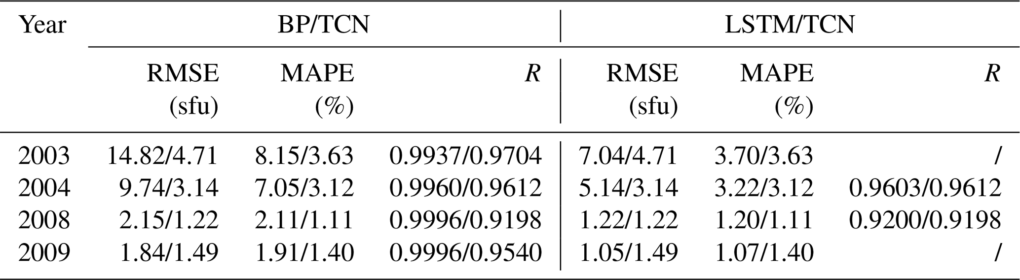
A comparison of the TCN model with other commonly used neural network models, like the BP model (Xiao et al., 2017) and LSTM model (Zhang et al., 2022), for prediction 3 d ahead is shown in Table 4. The RMSE of BP and LSTM models in predicting F_10.7 in the high-solar-activity year of 2003 is 14.28 sfu and 7.04 sfu, respectively. However, the RMSE of the TCN 3 d ahead is 4.71 sfu in 2003. The mean absolute percentage error (MAPE) of BP and LSTM models in predicting F_10.7 in the low-solar-activity year of 2009 is 1.84 and 1.05, respectively. However, the MAPE of the TCN 3 d ahead is 1.49 in 2009, which is better than that of other classical models. The TCN model predicts F_10.7 better than the LSTM and BP model. There could be three reasons for such results. Firstly, the TCN model uses a structure of convolutional layers and residual connections, which enables it to better capture long-term dependencies in time series data (Bai et al., 2018). In comparison, although the LSTM model can also handle long-term dependencies in sequential data, its gated unit structure may not fully capture the complex nonlinear relationships in the data (Zhang et al., 2022). On the other hand, the BP model is simpler and lacks specialized structures for handling time series data, which may result in an ineffective capture of temporal features (Xiao et al., 2017). The residual connections in the TCN model can help mitigate the vanishing gradient problem and improve the stability of the model. This is particularly important for long-term prediction tasks, as the model needs to propagate gradients through multiple time steps. In contrast, the LSTM model may encounter issues of vanishing or exploding gradients in long-term prediction, leading to difficulties in training and unstable predictions (Zhang et al., 2022). The BP model, as a traditional feedforward neural network, may also face similar problems. The TCN model possesses higher flexibility and adaptability, being able to automatically learn appropriate feature representations based on the characteristics of the data. In comparison, the LSTM and BP models require manual feature design and selection, which may not fully leverage the information in the data. The adaptive nature of the TCN model helps it better adapt to different time series data and improve the accuracy of predictions. Therefore, it is precisely because of the advantages mentioned above that the TCN performs better in F_10.7 prediction.

4 Conclusion

The F_10.7 solar flux is an important indicator of solar activity. Its applications in solar physics include serving as an indicator of solar activity level and predicting solar cycle characteristics. In view of the long observation time and certain periodicity of F_10.7, this paper introduces, for the first time, the theory and technique related to the TCN based on machine learning into the F_10.7 sequence prediction of space weather.

Firstly, we analyze the ability of the TCN model to predict daily F_10.7 during solar cycle 24 using training samples from 1957 to 1995. In addition we use the leave-one-out method for cross-validation. The results show that the change of prediction accuracy of the model is related to the intensity of solar activity. The TCN model does not large affect the final F_10.7 forecasts due to specific properties of the data. This proves that the TCN model is robust to some extent.

Secondly, we compared the predictive performance of the TCN model with the SWPC forecast results and autoregressive (AR) model forecast results. The results show that the TCN model outperformed the SWPC and AR models in terms of prediction accuracy. The predictive accuracy of the TCN model does not significantly vary with the lead time of short-term forecasts (1, 2, and 3 d). This demonstrates the stability of the TCN model's predictions.

Thirdly, the TCN model has been compared to other classic models such as the BP model and the LSTM model. The TCN model outperformed these models with a lower root mean square error (RMSE) and mean absolute percentage error (MAPE). This validates the effectiveness and reliability of the TCN model in predicting the F_10.7 solar radio flux. The TCN model is capable of capturing sudden increases or decreases in F_10.7, indicating extreme enhancements in solar activity. Therefore, the TCN model has significant implications for predicting F_10.7, as it can help us better understand and forecast changes in solar activity.

Although the TCN method has proven to be a viable method for predicting F_10.7, there is still room for further improvement in its predictive ability. Future work could attempt to introduce the variable of sunspot number into the model and use a more scientific approach to improve the generalization ability of the model.