Auroral breakup detection in all-sky images by unsupervised learning

Due to a large number of automatic auroral camera systems on the ground, image data analysis requires more efficiency than what human expert visual inspection can provide. Furthermore, there is no solid consensus on how many different types or shapes exist in auroral displays. We report the first attempt to classify auroral morphological forms by an unsupervised learning method on an image set that contains both nightside and dayside aurora. We used 6 months of full-colour auroral all-sky images captured at a high-Arctic observatory on Svalbard, Norway, in 2019–2020. The selection of images containing aurora was performed manually. These images were then input into a convolutional neural network called SimCLR for feature extraction. The clustered and fused features resulted in 37 auroral morphological clusters. In the clustering of auroral image data with two different time resolutions, we found that the occurrence of 8 clusters strongly increased when the image cadence was high (24 s), while the occurrence of 14 clusters experienced little or no change with changes in input image cadence. We therefore investigated the temporal evolution of a group of eight “active aurora” clusters. Time periods for which this active aurora persisted for longer than two consecutive images with a maximum cadence of 6 min coincided with ground-magnetic deflections, and their occurrence was found to maximize around magnetic midnight. The active aurora onsets typically included vortical auroral structures and equivalent current patterns typical for substorms. Our findings therefore suggest that our unsupervised image clustering method can be used to detect auroral breakups in ground-based image datasets with a temporal accuracy determined by the image cadence.

1 Introduction

Auroral displays exhibit a vast range of different morphologies and dynamics. Despite decades of research and an early morphological “template” for auroral evolution during substorms (Akasofu, 1964), there are still many unexplained structures and periods of evolution, as pointed out by Knudsen et al. (2021) in a recent review. With the fast development of observational capabilities, recent observations have also revealed new auroral (or similar) forms (e.g. Lumikot – McKay et al., 2019, Fragments – Dreyer et al., 2021, or STEVE – MacDonald et al., 2018), which emphasizes how we still lack knowledge and understanding of auroral structures and, in particular, their relation to each other.

One of the first automatic image classification attempts by Syrjäsuo and Donovan (2004) detected “arcs”, “patches” and omega bands. They stated that, for less than 10 % of all the auroral structures, the form is “known” and can be named. This obviously hampers our skills in performing morphological classification of aurora in a statistical sense and by means of supervised learning. The (known) structures typically included in supervised learning as the ground truth are arcs, patchy or diffuse, discrete, Moon and clouds (e.g. Clausen et al., 2018; Kvammen et al., 2020; Sado et al., 2022). These automatic classification results are good within about a 90 % success rate, but some of the commonly used auroral classes are very broad, with arcs and patches being the only specific shape and the rest of the auroral morphology being grouped into “discrete” and “diffuse” aurora. Furthermore, as about 50 % of the image data do not contain aurora (but rather clear skies, clouds or the Moon), classifying a combination of auroral and non-auroral classes makes the morphological part of the classification inefficient. To overcome the problem of classifying largely unknown auroral features, an auroral arciness index was introduced to include all images containing aurora (Partamies et al., 2014). This method recognizes all auroral structures and gives them an index-like number between 0.4 and 1 based on the distribution and clustering of the brightest pixels in the images. This method has been used to characterize the temporal evolution of selected known structures (e.g. poleward-moving auroral forms of the dayside aurora by Goertz et al., 2022).

An unsupervised learning attempt of the dayside auroral structures by Yang et al. (2021) clustered auroral forms into two categories based on 4000 randomly selected images over five auroral (northern winter) seasons. The number of clusters chosen by the authors was based on visualization of the feature vectors. As daytime aurora has previously been divided into four categories by human experts (e.g. Hu et al., 2009), the new unsupervised clustering results reopen the discussion on the unknown number of true clusters. In their study, the first cluster contained variable morphological features, such as arcs, patches and spots with high brightness and primarily afternoon occurrence, while the second cluster consisted of a corona-type aurora of lower brightness and high occurrence rate around magnetic noon.

To the best of our knowledge, we report the first attempt on unsupervised learning on auroral image data that includes both daytime and nighttime aurora. Our practical application is to automatically identify auroral breakups in the image data. This is particularly important for locations like the Svalbard archipelago. Surrounded by a highly conductive ocean, the ground-magnetic measurements are typically contaminated by the magnetic contribution of ground-induced currents by about 50 %–70 % (Juusola et al., 2020), making the traditional substorm onset detection methods on magnetic data less reliable.

2 Auroral image data

We use full-colour all-sky camera (ASC) data from Kjell Henriksen Observatory (KHO, 78.25° N, 16.04° E) on Svalbard in Arctic Norway. Our ASC is a Sony α7s mirrorless DSLR, which has been in operation since late 2015 but which has also had comparable predecessors since 2008. The ASC raw data have a high pixel resolution (2832 × 2832). However, our analysis uses quicklook data with reduced pixel and time resolution for faster processing. Nighttime images with 4 s exposure time have been taken at a cadence of 12 s throughout winter seasons, which on Svalbard extend from the beginning of November until the end of February. Images are captured when the Sun is below the horizon.

Daily summary plots of image data are automatically published in the form of keograms (http://kho.unis.no/Keograms/keograms.php, last access: 19 April 2024). These are north–south slices of individual images stacked together into daily time–latitude (or zenith-angle) plots. Keograms are used later on in the study to validate the results of our automatic classification.

In addition to the auroral image data, we use geomagnetic index data and solar wind data from OMNIWeb (https://omniweb.gsfc.nasa.gov, last access: 19 April 2024) to provide an overview of the magnetic activity level as well as a reference for comparisons between what we call “active” and “quiet” auroral displays (for more detailed explanations, see Sect. 4.1). Dst-index data from the World Data Center in Kyoto (https://wdc.kugi.kyoto-u.ac.jp/dstdir/index.html, last access: 19 April 2024) are used as a storm indicator. The Hp30 index (https://kp.gfz-potsdam.de/en/hp30-hp60, last access: 19 April 2024) (Yamazaki et al., 2022) gives a 30 min resolution version of the planetary Kp index, and the SuperMAG electrojet index (SML, https://supermag.jhuapl.edu/indices/, last access: 19 April 2024; Gjerloev, 2012) describes the auroral electrojet variability with a global coverage of magnetometer stations at 1 min resolution.

3 Classification method

3.1 Preprocessing of the auroral images

Manual labelling was performed for all quicklook images from the winter season 2019–2020 as well as for January and February 2019; quicklook images have a reduced resolution of 480 × 480 pixels and about a 6 min cadence. The manual labelling aimed to provide a ground truth for developing an automatic classification routine to detect images which contain auroral emission. This dataset contained approximately 37 000 labelled images. From this dataset, only those images that contained auroral emission and that were not dominated by clouds were further used in unsupervised learning. This became approximately 12 000 images.

To prepare the images for unsupervised learning, each image was first processed to remove features that could lead to biases that are unrelated to the auroral morphology, such as a caption indicating the camera type, observatory location, date and time. After removing the caption, images with very faint or barely detectable aurora were removed. In the quicklook images, the colour of each pixel is represented by individual intensities in red, green and blue colours. This is commonly known as the RGB colour space. However, for processing based on brightness, we transform the RGB colours into the HSV and L*a*b* colour spaces, where the brightness and actual colour content are more clearly separated.

In the HSV-colour space, the colours are expressed by the hue (H) and saturation (S), while the brightness is contained in the value (V) (Malacara, 2002). If V was less than 50 out of 255 in more than 90 % of the pixels in the image, the image was discarded as too faint. This left 10 300 images containing sufficiently bright aurora.

The L*a*b*, or CIELAB colour space, aims to represent the colours as a human observer would perceive them (Malacara, 2002). Here, L* denotes the lightness of the colour, while a* and b* provide the colour information. Unlike RGB and HSV, L*a*b* is a device-independent colour space based on a standard human observer and standard outdoor illumination. Similarly to earlier work (e.g. Sado et al., 2022; Clausen et al., 2018; Johnson et al., 2021), we clipped the L* values to the range from the 0.5th to 99.5th percentiles. To reduce the influence of the background sky conditions on the auroral classes, the median values of the a* and b* colour channels were used to provide a neutral white balance for all the images. Next, the images were cropped to 400 × 400 pixels around the center. This removes the biases due to dark corners outside the circular field of view of the all-sky images. This step also removes most of the auroral emission at the lowest elevation angles, which is beneficial as the morphology of the auroral forms near the horizon is heavily distorted by the fish-eye optics and is therefore difficult to examine.

To better take into account faint aurora, a contrast enhancement was performed on the images by equalizing the histograms of the L* channel for each image. Furthermore, a 5 × 5 median filter was used to remove single bright pixels due to stars, similarly to the 3 × 3 filter used by Kvammen et al. (2020). Finally, the images were resized to 224 × 224 pixels and converted back to RGB, which is the expected format for most feature extractors.

As an example of the effect of the preprocessing steps outlined above, Fig. 1 shows two original quicklook images (left column) and the corresponding preprocessed images (right column). The images demonstrate the impact of cropping, where aurora close to the horizon is excluded, as well as the effect of the colour enhancement and brightness normalization.

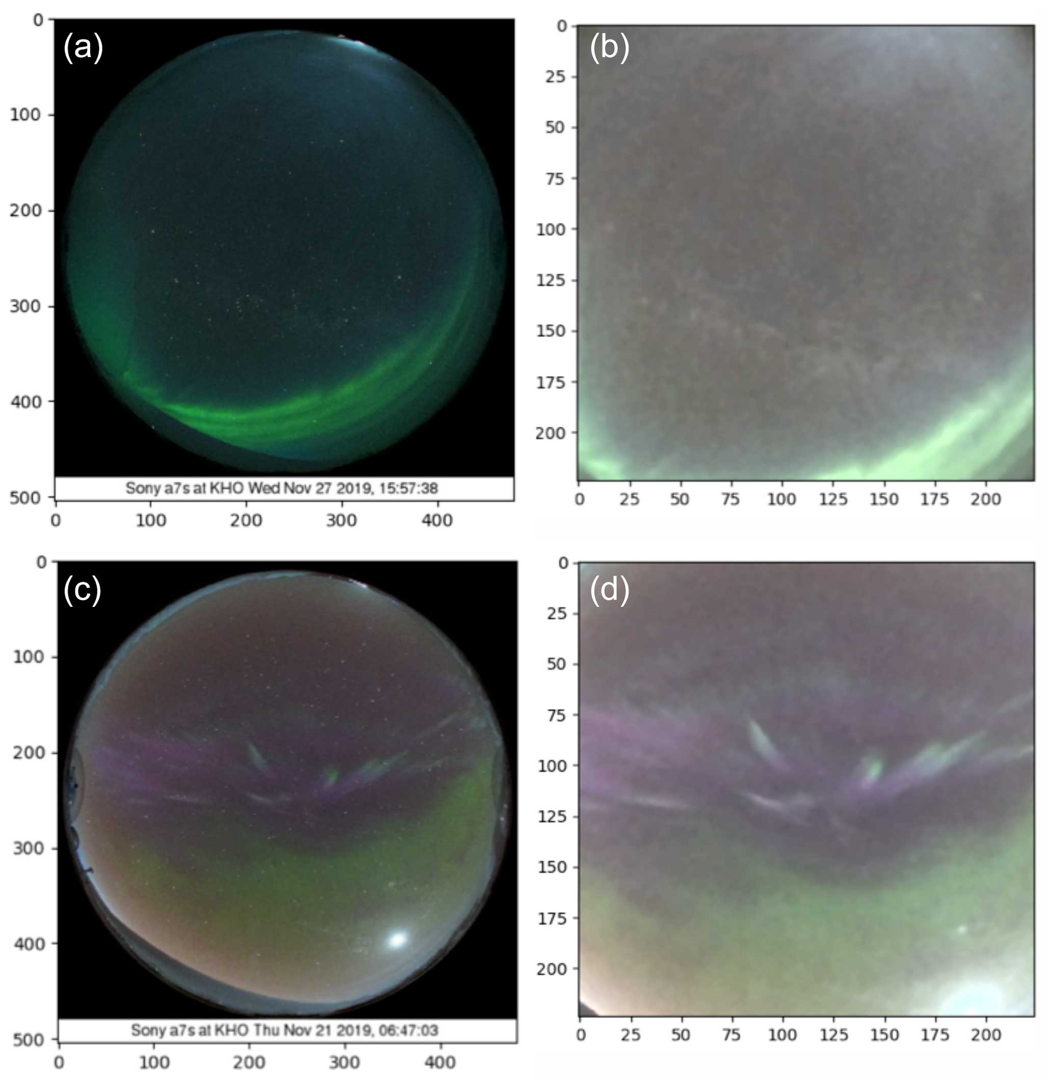
Figure 1 (a, c) Two quicklook images in their original format. (b, d) Corresponding images after the preprocessing steps of colour enhancement, brightness normalization, cropping and scaling.

The cadence of 6 min of the quicklook data favours quiet aurora over active aurora. This happens because active aurora occurs in short highly dynamic bursts, which are poorly sampled by a cadence of 6 min, while quiet aurora experiences longer lifetimes. To study the influence of this bias and to better represent the active auroral forms, a second dataset was created. In this dataset, the cadence was reduced to 24 s during selected periods of active aurora. This additional dataset is also referred to as a high-resolution dataset in this work. These selected periods were visually identified as the 19 brightest auroral displays with a large north–south extent as seen in the keograms (sample keogram in Fig. 5a).

3.2 Classification of images

In contrast to supervised learning, where we know the correct answer to a classification question and can train a classifier accordingly, in unsupervised learning we do not know the answer. The manual labelling of auroral images provided us with a dataset of unknown auroral forms. We try to learn the types of aurora in the data by using clustering algorithms. Intuitively, similar auroral shapes in the images should belong to the same cluster.

The first step is to define a numerical measure of the image content in the form of a feature vector. In the second step, the images are clustered based on their feature vectors: here, the true number of clusters is, of course, unverifiable. As clustering is often based on similarity metrics, the results also depend on how well the feature vectors represent the image content. In his Master's thesis, Teissier (2022) evaluated a number of different feature vector extractors as well as clustering approaches. The following provides a brief description of the central concepts and choices of the methodology.

Classifiers based on convolutional neural networks (CNNs) (LeCun et al., 2015) are becoming increasingly popular in image analysis. Training an artificial neural network refers to the process of optimizing all parameters within the network to minimize the classification error.

The analysis of auroral images in our dataset uses a processing chain which includes a CNN architecture followed by a smaller neural network. We start with the inclusion of high-time-resolution data as they provide a better balance between images of auroral displays during active and quiet times. We use a variation of the SimCLR feature extractor used by Johnson et al. (2021). This feature extractor builds on the Resnet-50 neural network (He et al., 2016) architecture. Random rotations and other image transformations are often used in training image classifiers to both artificially increase the number of “different” sample images and to obtain invariance in orientation. In this study, we limit ourselves to horizontal flipping (east–west in auroral images) and random cropping (random parts of the sky with aurora) in the training phase (Teissier, 2022).

We used the UMAP (uniform manifold approximation and projection for dimension reduction) method to reduce the dimensionality of the feature vectors (McInnes et al., 2020). This step was carried out to improve clustering (Steinbach et al., 2004). In the UMAP reducer, there are two critical parameters: one impacting how much the algorithm focuses on local versus global structures (N_neighbors) and another determining the minimum allowed distance between the features in the dimensionally reduced space (min_dist). Based on the experiments by Teissier (2022), we used the values N_neighbors=20 and min_dist=0.

Finally, a clustering algorithm was used to determine clusters of the dimensionally reduced feature vectors. Two different clustering algorithms were used: K-means (MacQueen, 1967) and hierarchical (Nielsen, 2016) clustering. These algorithms were used to divide images into 30 or 100 clusters. Consequently, the four clustering results (two clustering algorithms and two numbers of clusters) were fused together to balance the weaknesses and biases of the individual approaches. This also helps to identify outlier images that are connected to different auroral features, depending on the clustering algorithm that is used. The fusion was done by using modified majority voting with a co-association matrix algorithm (Fred, 2001). The original algorithm was modified to have two tuneable parameters. The first parameter is the majority threshold of the co-association matrix, above which two samples are merged in the same cluster. The second parameter is the minimal cluster size, under which a cluster is merged into a cluster of “outliers” to indicate hard-to-classify images. The values of these parameters were determined by changing them to minimize the loss function

$$\begin{array}{}\text{(1)}& \begin{array}{rl}& L={\displaystyle \frac{\mathrm{1}}{n_{\mathrm{c}}}}\sum _{k=\mathrm{0}}^N|n_k-n_{\mathrm{0}}^k|+{\displaystyle \frac{n_e}{n_{\mathrm{c}}}}\mathrm{with}{n}_{\mathrm{0}}^k={\displaystyle \frac{N}{n_{\mathrm{c}}}}\mathrm{if}k<n_{\mathrm{c}},\\ & \mathrm{otherwise}{n}_{\mathrm{0}}^k=\mathrm{0},\end{array}\end{array}$$

where N is the total number of samples, n_k the number of samples in cluster k and n_e the number of outlier samples. Parameter n_c is used to influence the number of clusters resulting from the fusion and was set to 25. The fusion resulted in 37 clusters with numbers ranging from −1 to 35, where the −1 cluster is for the outlier images not belonging to any of the other clusters.

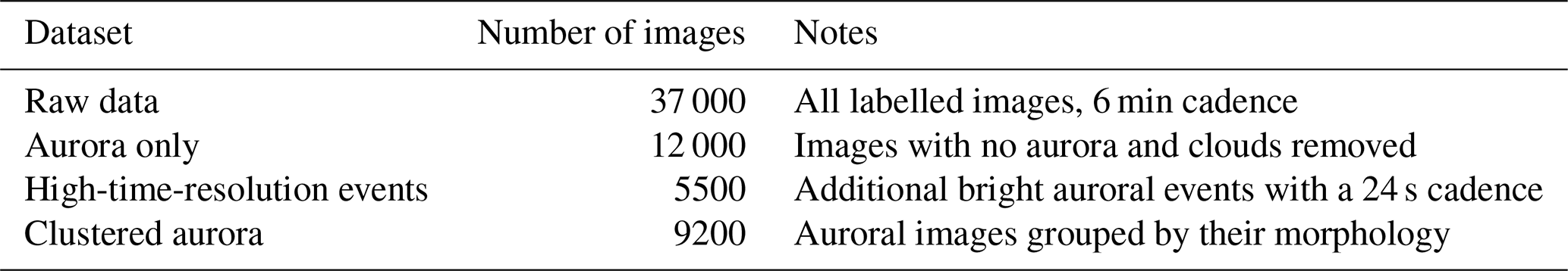
Using a basic desktop computer (in 2022), the preprocessing, training and clustering required roughly 1 d of computer time. Predicting clusters for additional images takes less than 1 s per image. Table 1 summarizes the numbers of images at each stage of the data processing.

Table 1 Summary of numbers of images in our datasets throughout the process.

4 Results

4.1 Differences between active and quiet aurora

The CNN analysis was run on the quicklook images with a 6 min cadence alone as well as on the full dataset with the inclusion of higher-resolution images with a 24 s cadence. As a result, we found that the occurrence of some morphological clusters increased greatly with the increasing temporal resolution, while the occurrence rate of the other clusters was nearly unaffected.

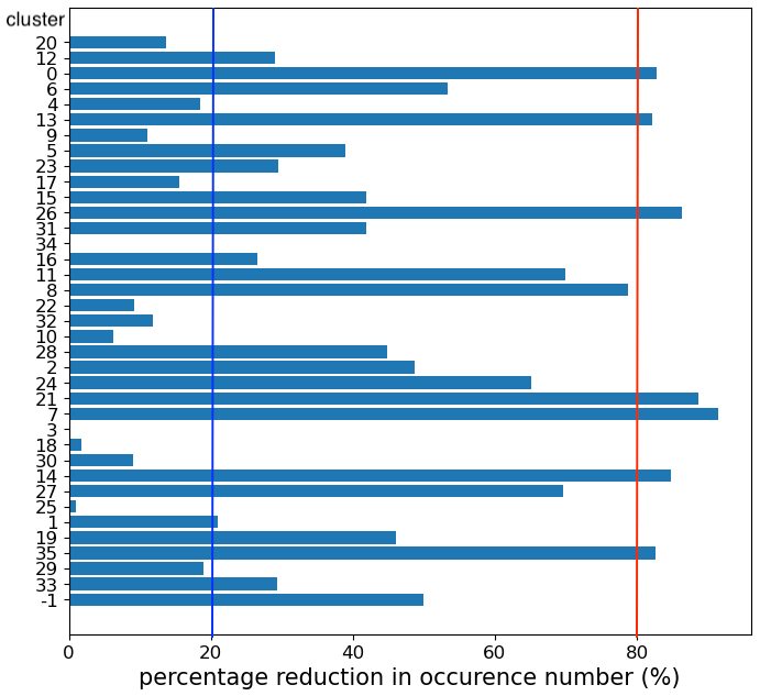
Figure 2 Occurrence rate difference of all 37 clusters between quicklook and high-resolution data in percentage with respect to the total occurrence rate of each cluster. Clusters with a maximum change of about 20 % are called quiet aurora, and clusters with at least about 80 % change are called active aurora. Threshold occurrence changes for quiet and active aurora are marked by the blue and red vertical lines, respectively. Cluster number −1 is an outlier cluster. Figure according to Dol (2023).

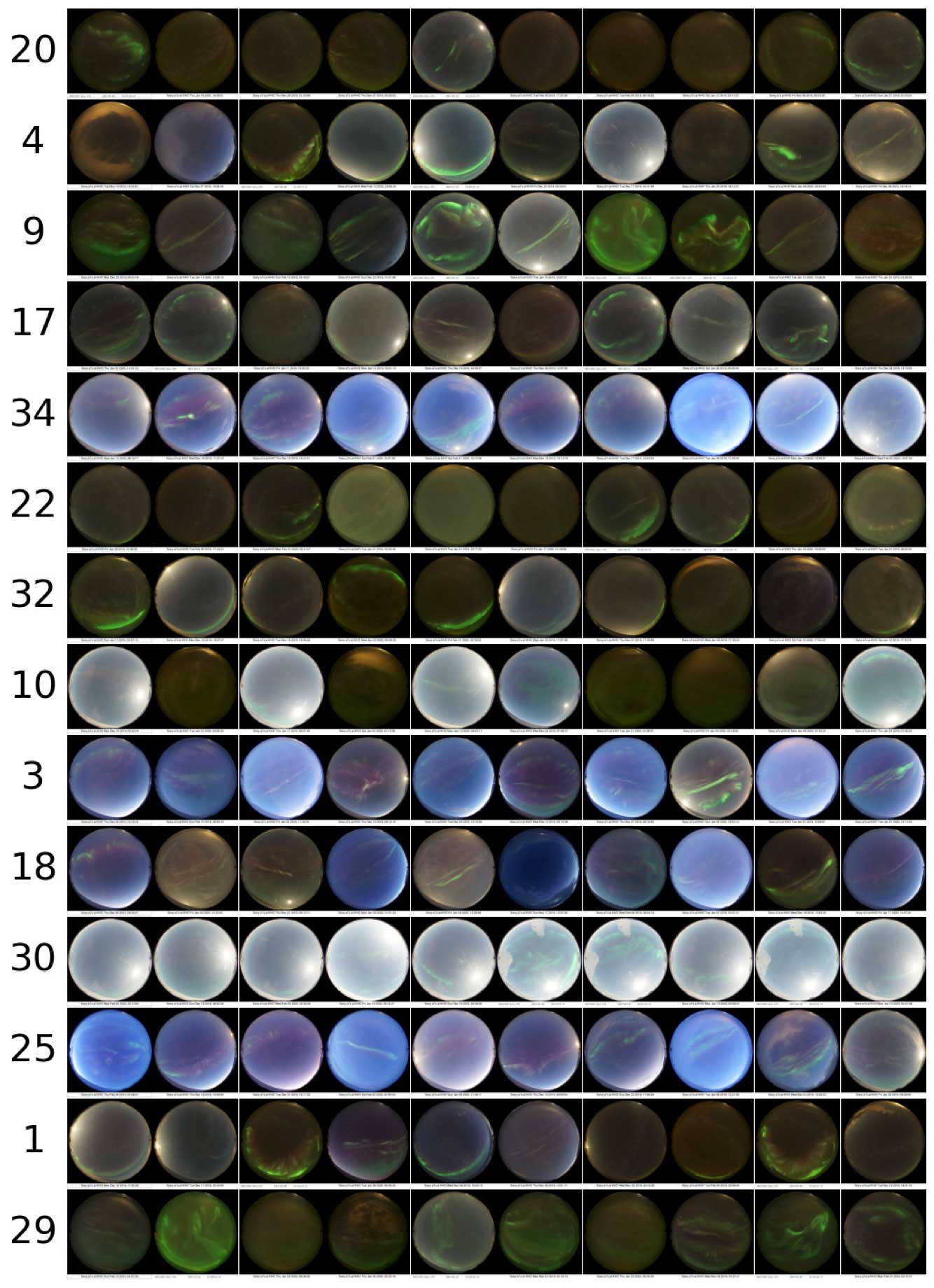
The high sensitivity to the increased temporal resolution in the image data (at least about an 80 % change, red vertical line in Fig. 2) suggests that these clusters primarily describe the morphology of active auroral displays. These are the cluster numbers 0, 13, 26, 8, 21, 7, 14 and 35. The occurrence change of the individual clusters is illustrated by Fig. 2. It shows the occurrence rate difference of all 37 clusters between quicklook and high-resolution data in percentage with respect to the total occurrence rate of each cluster. The clusters, for which the occurrence showed little or no change (maximum of about 20 % change, blue vertical line in Fig. 2) with the increasing temporal resolution (cluster numbers 20, 4, 9, 17, 34, 22, 32, 10, 3, 18, 25, 1 and 29), are likely to contain auroral structures mainly related to quiet auroral displays. By quiet auroral displays, we refer to images of structures which are relatively simple, are dim and evolve slowly in time. A typical example of this is an auroral arc, or a multiple arc, which changes little between consecutive images with a higher temporal resolution of 24 s. A set of 10 randomly selected images from each of the individual clusters included in quiet aurora is shown in Fig. 3. In addition to the simple green auroral structures, daytime and afternoon overhead aurora with a notable red emission contribution belongs to this category.

Figure 3 Ten random images from each individual cluster included in the category of “quiet aurora” (Dol, 2023).

Active auroral displays, in turn, refer to images with one or multiple more complex auroral structures, which evolve significantly between consecutive images in our higher-temporal-resolution dataset and have little resemblance between consecutive images at quicklook time resolution (6 min).

Figure 4 Ten random images from each individual cluster included in the category of “active aurora” (Dol, 2023).

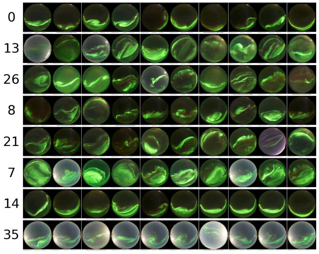
A random selection of images in each individual cluster included in active aurora is displayed in Fig. 4. These active auroral displays typically include bright emissions in vortical, rayed and small-scale structures. The threshold values for the occurrence rate changes for quiet and active aurora (∼ 20 % and ∼ 80 %, respectively) are based on visual inspection of the cluster occurrence rate histogram in Fig. 2 and are therefore somewhat arbitrary. Note that cluster number 1 is included in the quiet aurora, although its change rate is just over 20 %. Similarly, cluster number 8 is included in the active aurora, although its change rate is just under 80 %. These choices were made with the idea that a large percentage difference is a conservative choice as long as it results in several clusters in each extreme.

From image samples in Figs. 3 and 4 it is obvious that a detailed description of the type of aurora in each individual cluster is difficult to determine. Simple properties, such as the brightness, contrast, colour, alignment or location of the aurora in the image, seem to play a role in the numerical clustering. For both the quiet and active aurora categories, the images containing the Moon have been collected in the same clusters. Any more detailed interpretation of the individual clusters will require more analysis.

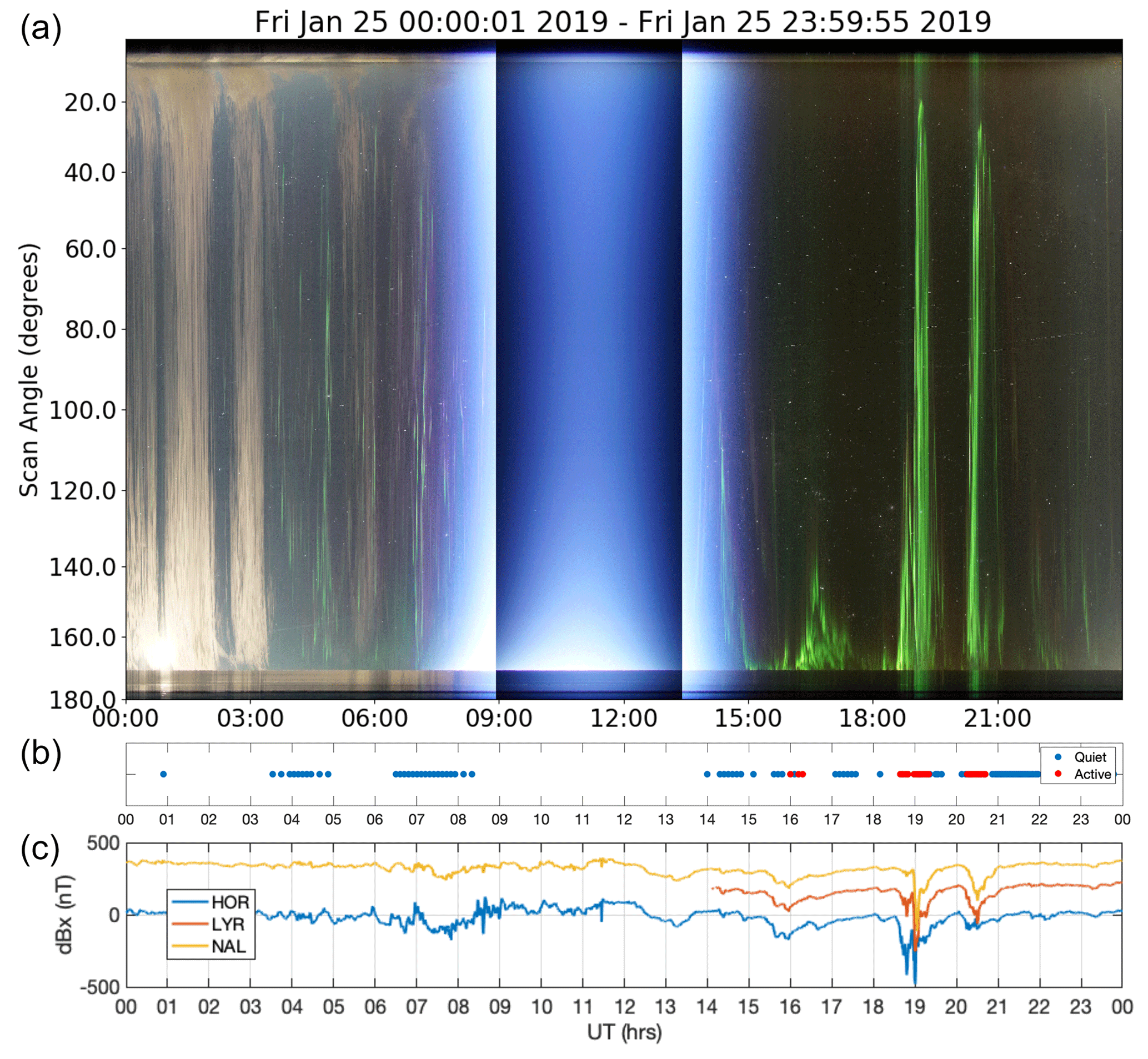
Figure 5 (a) Sample keogram of colour ASC data on 25 January 2019. At 00:00–01:00 UT in the southern sky (at scan angles 160–180°), the moon is visible and illuminates the clouds in the field of view. At 03:00–08:00 UT a faint morning sector aurora is seen, first as green and later also as red. At 08:00–15:00 UT the daylight increases the illumination of the sky, although the Sun is below the horizon. Due to the increased light level, the exposure time changes, and this is seen as vertical colour changes at about 09:00 and 13:30 UT. From 15:00 UT onwards the sky is dark and a green aurora appears in three northward expansions. (b) Time series of active (red dots) and quiet (blue dots) aurora for the sample day. (c) Evolution of ground-magnetic X-component deflections at the stations of NAL (yellow), LYR (red) and HOR (blue). LYR data are missing until 14:00 UT but exist during the active auroral displays.

An example of the time evolution of auroral all-sky image data with the detected active and quiet auroral displays is provided by Fig. 5a, which is a full keogram of 25 January 2019, and Fig. 5b, which shows the time evolution of individual images of active (red dots) and quiet (blue dots) auroral displays. The images of active and quiet aurora are most frequent in the time periods of clear skies and aurora, because our preprocessing excludes clear skies with no aurora and images with clouds. Active aurora coincides with the brightest aurora in the keograms, as expected. Figure 5b shows ground-magnetic data (X component) from the Svalbard magnetometer stations in Hornsund (HOR, 77.00°Glat), Longyearbyen (LYR, 78.20°Glat) and Ny-Ålesund (NAL, 78.92°Glat). These stations are part of the IMAGE magnetometer network (https://space.fmi.fi/image/www/index.php, last access: 19 April 2024) (Tanskanen, 2009). The magnetic variations are measured and plotted at 10 s time resolution. The three periods of active aurora correspond to small (∼ 100 nT) to moderate (∼ 400 nT) magnetic deflections in the north–south component. They could all be interpreted as substorms, the first of which expands towards Svalbard from further south, while the latter two events occur more directly overhead. The visual correspondence between the periods of active aurora and the magnetic deflections during the latter two substorms appears particularly good.

To further investigate these different morphological cluster groups of “active” and “quiet” aurora, we selected time periods of active or quiet aurora that included three or more consecutive images with a maximum cadence of 6 min. For a sequence longer than three consecutive images, one single quiet-class image would be allowed within an active aurora period, or the other way round. This procedure resulted in 28 active aurora events and 222 quiet aurora events in the time frame of all our labelled data in 2019–2020.

Table 2 Median values of event durations, geomagnetic indices and solar wind speeds for periods of active and quiet aurora, respectively.

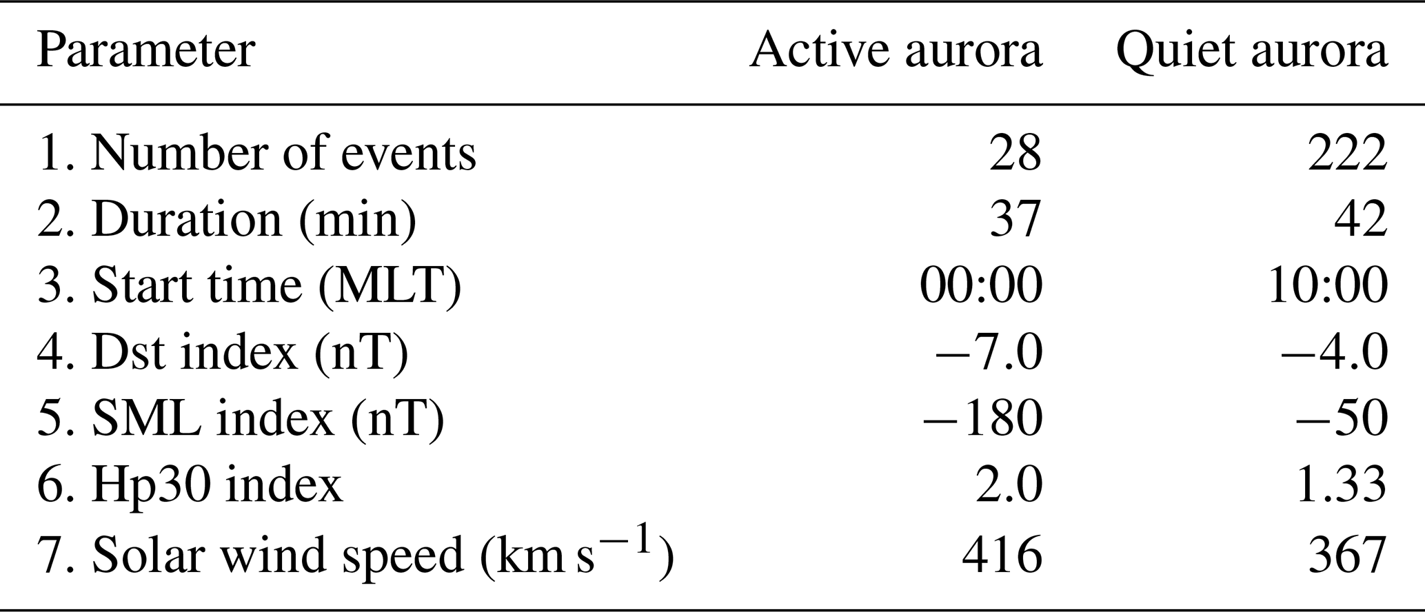
Table 2 gives an overview of the typical parameters for periods of active and quiet aurora. The duration of the active aurora events varied from 60 s to 5 h, while that of the quiet events ranged from 2 min to 25 h. The median values (row 2 in the table), however, do not differ much. The active aurora events typically started at magnetic midnight (row 3), while the quiet aurora events were spread more evenly over the magnetic local time (MLT) hours, which is illustrated by Fig. 6. The median start time is therefore not a good indicator of quiet aurora, which experiences three occurrence maxima in 24 h: right after midnight, at about 06:00–09:00 MLT and at about 15:00–19:00 MLT.

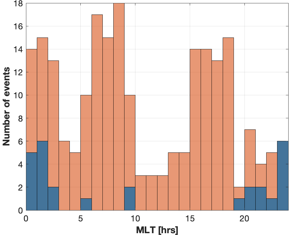
Figure 6 Distribution of the start times of active (blue) and quiet auroral displays (orange) (MLT). Midnight in magnetic local time is about 21:00 UT on Svalbard.

The geomagnetic indices with coarser spatial resolution (a low number of stations, which provide the data) are not dramatically different between the periods of active and quiet aurora. These are the Dst index (row 4) and the Hp30 index (row 6). Neither of these indices with low spatial resolution includes high-latitude magnetic field data, and therefore they do not reflect the high-latitude magnetic deflections, which may have different timings compared to the corresponding deflections at lower latitudes. However, the SML electrojet index (row 5), which has good spatial coverage of magnetic data from a range of different latitudes, shows a difference of more than 100 nT between active and quiet aurora. Similarly to the low-resolution magnetic indices, the median solar wind speed (row 7) is more enhanced during active aurora than quiet aurora, but only by some tens of kilometers per second, which is not significant.

4.2 Are the active aurora periods auroral breakups?

We performed a visual inspection of what the active aurora periods correspond to by using keograms (as in Fig. 5a). The main mission of the validation procedure was to find out what the detected events looked like, whether they corresponded to magnetic substorm activity, whether keogram inspection could reveal missed auroral activations, and, if yes, what kind of events they would be. Keograms were therefore viewed for each day from January 2019 until March 2020. We inspected all detected active aurora events as well as each keogram for any additional auroral brightening, which was not detected.

Most active aurora periods were auroral brightenings for which the bright emission extended over the full (or nearly full) field of view of the all-sky image, as illustrated by the keogram in Fig. 5a. Most of the active aurora periods also coincided with a small to moderate deflection of the local magnetic north–south (X) component, which indicates substorm activity. The maximum magnetic deflections for the active aurora events ranged from about 50 nT up to about 400 nT, with a median value of 100–200 nT. Cluster numbers of individual images were also investigated during the active aurora periods, but no consistent time evolution or preferential order was found among the individual active aurora clusters.

Taking the auroral breakup overhead as a benchmark, five false-positive events were identified in the visual inspection. Three of our false-positive cases were morning sector auroral events (see the lonely blue bars in Fig. 6). These consisted of transient brightenings in the morning sector diffuse and pulsating aurora. Two of these events are from the shortest end of the duration spectrum containing only two consecutive images. This type of event could be filtered out simply by increasing the minimum duration of the active aurora events in order to produce a cleaner auroral breakup list. Two of the other events we call false-positive cases were clearly substorm-like aurora which extended about halfway in the sky towards the local zenith, such as the first active aurora event in Fig. 5. These types of events are not exactly wrongly detected but are rather a milder category compared to the rest of the cases. They may include substorms, which inherently do not take place at high latitudes but rather expand towards Svalbard from further south, where the strongest magnetic disturbances take place.

As for false negatives, i.e. any additional auroral brightenings that the active aurora periods did not cover, no events were found. Based on keograms, we visually identified some auroral brightenings that nearly extended across the full sky but that were not automatically identified as active aurora. These included (1) events where the sky was fully or partly cloudy, so that the auroral structures were obscured; (2) events where the image was contaminated by moonlight, so that the auroral brightness (and therefore the structure) was not very visible; and (3) events which were substorm-like auroral activations that did not even reach halfway toward the local zenith. Images in the first two categories would have been excluded from the data fed to the classifier due to the clouds or the moonlight. In the last category, the largest magnetic deflections occurred typically further south of Svalbard, which was confirmed by visual examination of the IMAGE magnetometer data.

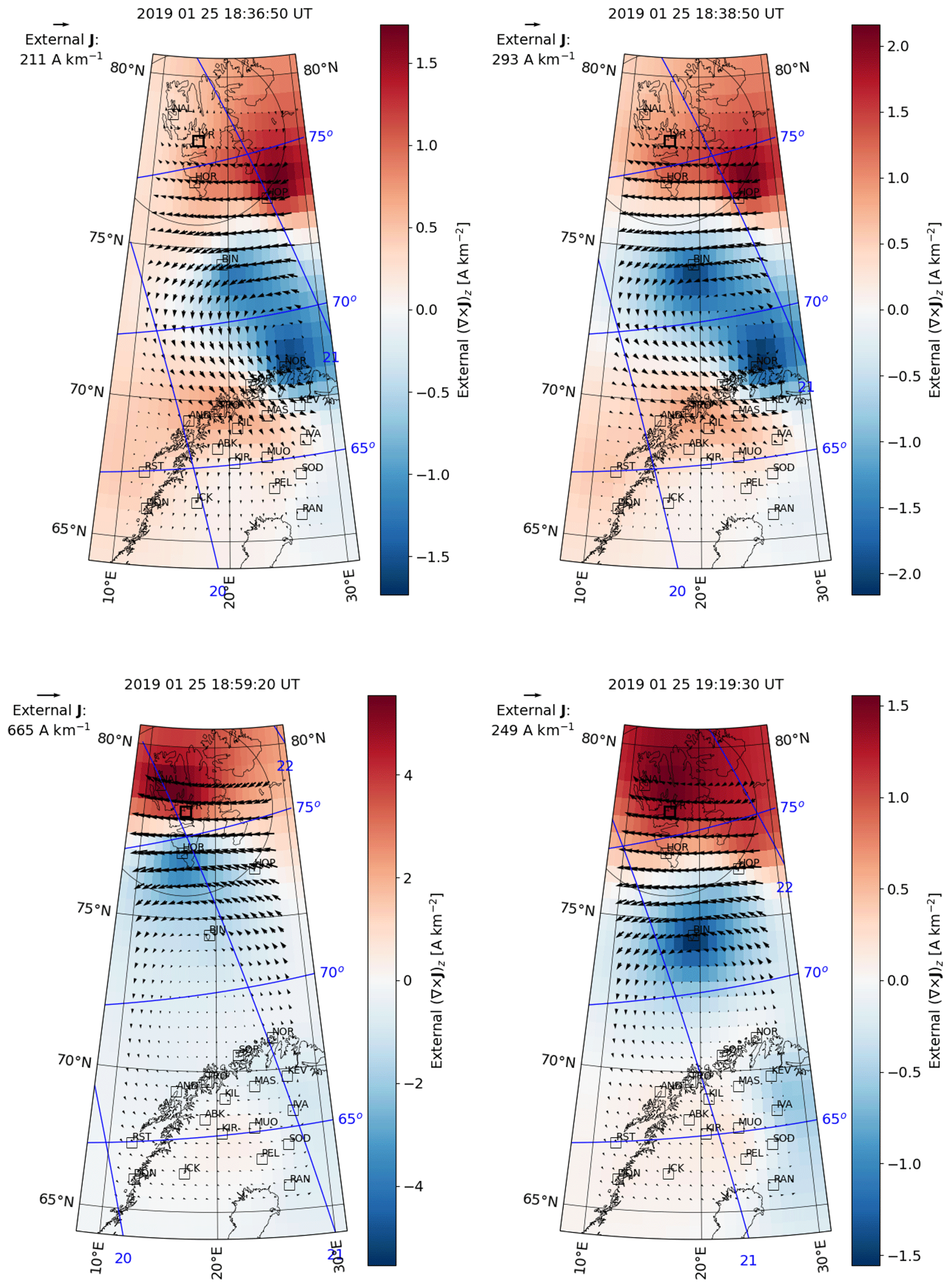
Figure 7 Ionospheric equivalent currents (Vanhamäki and Juusola, 2020) (arrows) and the Z component of their curl (colour) that can be interpreted as an estimate of field-aligned current j_Z on 25 January 2019, 2 min before a period of active aurora started (18:36:50 UT), at the start of the period of active aurora (18:38:45 UT), during the period of active aurora (18:59:20 UT) and at the end of the period of active aurora (19:19:27 UT). The IMAGE magnetometer stations used to construct the equivalent currents are shown by black rectangles and the LYR field of view by a circle. Magnetic apex coordinates (Richmond, 1995; Emmert et al., 2010; Laundal et al., 2022) are indicated by the blue grid.

Figure 7 shows snapshots of the ionospheric equivalent currents, derived from 10 s IMAGE magnetometer data (Vanhamäki and Juusola, 2020), on 25 January 2019 around a period of active aurora in Fig. 5. The plots show an equivalent current pattern typical for the westward traveling surge (WTS) (e.g. Vanhamäki et al., 2005) sweeping past LYR from southeast to northwest. Two minutes before the period of active aurora (18:36:45 UT), the U-shaped head of the surge pattern was still located south and east of the LYR field of view (indicated by the black circle). The surge head appears to reach LYR at the time the active aurora started (18:38:45 UT) and to disappear around the time the active aurora ended (19:19:27 UT). A similar sequence of equivalent current dynamics (not shown) can be seen around the next interval of active aurora (Fig. 5) between 20:18:14 and 20:41:04 UT. We have also examined several other active aurora events and found similar equivalent current development. This indicates that periods of active aurora may be associated with a WTS which originated earlier at a substorm onset location just east and south of LYR and which traveled westward and northward past LYR.

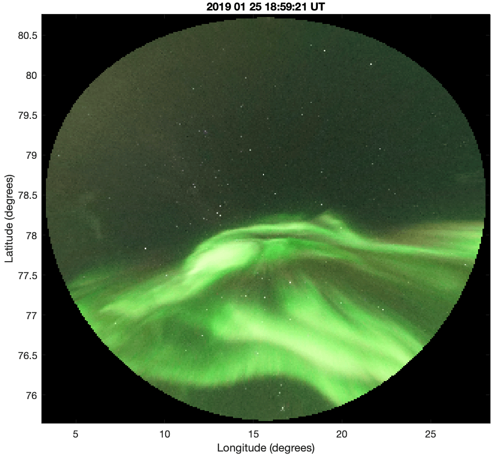
Figure 8 An image of the surge head taken at 18:59:21 UT plotted into geographic coordinates for easier comparison with the corresponding distribution of equivalent currents in Fig. 7. The assumed emission peak height for the mapping was 110 km.

Figure 8 shows the ASC image of the surge head aurora as it comes into the ASC field of view, which corresponds to the strongest ionospheric equivalent currents at 18:59:20 UT (Fig. 7). Here the image is plotted onto geographic coordinates to make it more comparable to the coordinates of the equivalent current maps (grey grid). Characteristics of the WTS aurora are the intense auroral emission and vortical structures located within the region of an upward field-aligned current (blue colour, negative external j_Z). The auroral evolution leading to this included poleward expansion from the southern edge of the field of view as well as more localized brightenings propagating from east to west along the poleward boundary of the surge aurora. This evolution is in agreement with that of the equivalent currents as described above.

5 Discussion

Results from our newly developed method for morphological clustering of auroral images have been used to detect auroral activations over Svalbard. While the method produced 37 individual clusters, which we cannot describe in detail, our further analysis suggests that the occurrences of eight of those clusters are associated with active auroral displays. Similarly, 14 clusters are prominently present during quiet auroral displays. A particularly interesting finding is that longer periods of active auroral displays practically include all full-sky auroral events in our all-sky field of view. These events coincide with ground-magnetic deflections and enhanced westward ionospheric electrojet currents, which are signatures of magnetospheric substorms. At high latitudes and close to the polar cap boundary, such as at Svalbard (78°Glat), auroral breakups overhead do not happen often. It is therefore practical to have a way of automatically identifying them in the image data in such a way that no events are missed, even when this means detection of some additional false positive cases (10 %–15 %).

The MLT distribution of quiet aurora in Fig. 6 has three maxima: one around midnight, one in the afternoon at 15:00–17:00 MLT and one in the morning at 06:00–09:00 MLT. This is in very good agreement with an MLT distribution of auroral structures for Svalbard in quiet geomagnetic conditions (Partamies et al., 2022). In their 13-year long data series, the auroral morphology was investigated in terms of simple auroral structures called auroral arcs versus other more complicated structures. Both classes undergo a similar MLT occurrence rate when geomagnetic conditions are quiet (the auroral electrojet AL index is larger than −100 nT). These quiet conditions correspond to the magnetic disturbance level for our quiet aurora. Similarly, for their active conditions (AL smaller than −300 nT), the MLT occurrence of both arcs and more complex auroral structures maximize between 21:00 and 02:00 MLT. This agrees with the occurrence of our active aurora, even though our active aurora events generally take place in less disturbed conditions (SML median of −180 nT).

An earlier study by Signh et al. (2012) analysed magnetic signatures of high-latitude substorms poleward of the central auroral oval. They concluded that the substorms occur primarily close to the MLT midnight, at 21:00–02:00 MLT during low or moderate solar wind streams, which is in very good agreement with the occurrence conditions of our events. In a more recent high-latitude substorm study, Cresswell-Moorcock et al. (2013) identified 112 events of energetic electron precipitation (EEP) in 12 months of electron density profiles from EISCAT Svalbard radar (ESR) measurements. This is a much larger number than what we collected in our study, but since our optical approach requires both dark and clear skies (possible for only 3 months a year), the event numbers seem comparable. Our events were collected from a total of 6 months of data, and statistically about half of the auroral images are cloudy. Our events of active aurora show a very similar occurrence around magnetic midnight, as do the EEP events detected in radar data (their Fig. 3a). Our auroral breakups occurred in less active magnetic conditions as compared to the EEP events from the radar data (the Kp or Hp index is 2 for ours and 3 for theirs) and during average solar wind speed, while the EEP events were reported to take place during fast solar wind. It is very likely that our auroral breakups will therefore not fulfill the EEP criterion of strong D-region ionization.

An automated method which would most closely compare to our approach is a new study on pixel-level classification that has empirically implemented thresholds for detecting auroral intensifications by Yamauchi et al. (2023). This method includes auroral breakups among other brightenings. What the authors call a local-arc brightening is not validated strictly as substorm activity, because brightenings take place at all local times. The pixel-level classification of a full-resolution ASC image requires a lot more manual work than manual labelling of full images, but since the authors used data from the same camera model as ours, a cross-validation of our results can be performed in the future.

ASC image data have been used to detect auroral breakups before. Murphy et al. (2014) developed a method which utilized the temporal evolution of the auroral image brightness as a proxy for auroral breakups. Three independently studied substorms were identified with good accuracy. Furthermore, 50 % of 240 independently listed substorm onsets were detected within the uncertainty of their method.

Currently, the only operational image classification method that runs on real-time image data is described by Nanjo et al. (2022). They use unpruned auroral colour images from Tromsø and Skibotn in northern Norway and Kiruna in northern Sweden (https://tromsoe-ai.cei.uec.ac.jp/, last access: 19 April 2024). The closest aspect of auroral breakup detection in that approach is the beginning of an extended period of the class called discrete aurora. The class itself contains much more than just the auroral breakups, but with some further analysis those results may also become a helpful cross-validation dataset for our method in the future.

While the results presented here are very promising, further research is needed to assess how efficiently this method works on unseen image data from different winter seasons. This essentially depends on how well the originally manually labelled image data from 2019 to 2020 represent all the different sky conditions and the variety of auroral morphology at and around the polar cap boundary. Also worth testing is whether the current results are sensitive to the use of brightness normalization in the preprocessing of the images. Specifically, one should investigate whether the brightness normalization leads to an unnecessary bias towards faint auroral structures. Future studies will also include testing of the method on other similar ASCs at different locations. This may require re-evaluation of the categories of active and quiet aurora, as individual instruments have slightly different colour balances, which may affect the clustering results. Furthermore, aurora at lower latitudes consists of different structures to some extent and will be limited to the nightside aurora with different emission balances and different background sky conditions as compared to the dayside aurora. All these factors may affect the occurrence of the morphological clusters and must therefore be investigated. The traditional way of detecting substorms is to use measurements of a ground-magnetic field. Because the magnetic data are not sensitive to weather or daylight conditions, the magnetometer station density is high and the data are available in long time series at high temporal resolution, the magnetic approach has been widely used for statistical studies (e.g. Forsyth et al., 2015; Partamies et al., 2013; Juusola et al., 2011). However, the recently documented ground-induction contribution in the magnetic measurements suggests that the magnetic substorm detection may be biased (Juusola et al., 2020). Furthermore, for some studies it is essential to include information on the auroral morphology, which makes the availability of the image data a key element.

6 Conclusions

This study has explored a newly developed prototype method for automatic clustering of auroral all-sky images in an unsupervised way. We used manually labelled data that were known to contain aurora, which means that in order for this approach to work, a classification of raw images into classes of “aurora” and “no aurora” is needed. Our method produced 37 clusters. Our results showed that an occurrence of a group of clusters was strongly increased with an increasing temporal resolution of input images taken during bright auroral displays. This indicates that a time sequence of these morphological clusters mainly describes auroral activations. This result was further used to detect the start times of periods with continuous auroral activity in our labelled data. Examination of the detected auroral activations showed that these are indeed local auroral breakups that carry substorm-like properties to the extent that high-latitude substorm events are expected to. An essential skill of our method is that no major events were missed by the detection. These are promising results that may help in identifying optical auroral breakups in the future after being tested on unseen data and cross-validated with other methods.