A technique for volumetric incoherent scatter radar analysis

Volumetric measurements of the ionosphere are important for investigating spatial variations of ionospheric features, like auroral arcs and energy deposition in the ionosphere. In addition, such measurements make it possible to distinguish between variations in space and time. While spatial variations in scalar quantities such as electron density or temperature have been investigated with incoherent scatter radar (ISR) before, spatial variation in the ion velocity, which is a vector quantity, has been hard to measure. The upcoming EISCAT3D radar will be able to do volumetric measurements of ion velocity regularly for the first time. In this paper, we present a technique for relating volumetric measurements of ion velocity to neutral wind and electric field. To regularize the estimates, we use Maxwell's equations and fluid-dynamic constraints. The study shows that accurate volumetric estimates of electric field can be achieved. Electric fields can be resolved at altitudes above 120 km, which is the altitude range where auroral current closure occurs. Neutral wind can be resolved at altitudes below 120 km.

1 Introduction

It would be of huge importance to measure the way in which electric fields in and around auroral arcs vary in time and space. This would allow us to gain new knowledge on the evolution of currents in Cowling channels, the closure of Birkeland currents and ultimately the dynamics of magnetosphere–ionosphere coupling in the auroral regions. To investigate the spatial variation of the ionospheric electrical fields and currents, it is necessary to measure how physical quantities vary over a volume in the ionosphere (e.g., McCrea et al., 2015).

Investigating the spatial variation of the ionosphere can be done in two different ways: multi-beam scanning or aperture synthesis radar imaging (ASRI). With multi-beam scanning, also known as volumetric imaging (Semeter et al., 2009; Nicolls et al., 2014; Swoboda et al., 2014, 2017), the radar beam is pointed in different directions to measure the local states in the ionosphere. Multi-beam scanning covers a large region in the ionosphere and is thereby useful for investigating large-scale structures. With ASRI, the phase difference in a received signal between receivers is used to investigate small-scale structures inside the radar beam (see e.g., Hysell and Chau, 2012). In this paper, we investigate the multi-beam scanning with EISCAT3D (E3D). For ASRI with E3D, we refer to Stamm et al. (2021b).

A phased array is an array of (dipole) antennas where the beam can be steered by changing the phase of the transmitted or received signals. Combined with electronic control of the phases at every antenna, the beam steering can be performed between two consecutive pulses (e.g., Wirth, 2001). The advanced modular incoherent scatter radars (AMISRs) (Valentic et al., 2013; Heinselman and Nicolls, 2008) were the first incoherent scatter radars (ISRs) that combined these two, making it possible to perform measurements of scalar ionospheric parameters, such as electron density n_e, electron temperature T_e and ion temperature T_i in some tens of seconds (Semeter et al., 2009). By assuming that the electric field along magnetic field lines is constant and that the field-aligned ion flow is completely constant, the variation in Doppler shift can be used to estimate horizontal variations in the electric field (Nicolls et al., 2014). However, full volumetric measurements of vector parameters require multiple receivers. At least one receiver for every component of the ion velocity vector is needed. This will be possible with E3D when it is finished (McCrea et al., 2015).

With the first three sites of E3D, volumetric measurements of ion velocity will become possible. The core site with combined transmitter and receiver is going to be in Skibotn, Norway, and two remote receiver sites are built in Kaaresuvanto, Finland, and Kaiseniemi, Sweden. Each site will have a phased array, which will be built with up to 109 hexagonal subarrays consisting of 91 crossed dipole antennas each. In Skibotn, 10 additional outrigger subarrays will be built for interferometry (Kero et al., 2019).

The technique for estimating electric field and neutral wind from ion velocity has been based on determining the electric field at high altitudes where the ion drift is dominated by E×B drift. Then, the electric field has been assumed to be constant along the magnetic field line so the neutral wind could be estimated at lower altitudes. This technique was introduced by Brekke et al. (1973) and has been used in many studies of the neutral wind (Brekke et al., 1974, 1994; Brekke, 2013; Heinselman and Nicolls, 2008; Nygrén et al., 2011, 2012). However, for analyzing a vector field, the method has to be adjusted because only one beam will be field-aligned.

In this work, we present a technique to estimate the 3D variation of electric fields and neutral winds from multi-static ISR measurements of ion velocities. A volumetric model makes it possible to use Maxwell's equations and the continuity equation for the neutral wind to constrain the estimates. The work is a 3D generalization of the work of Stamm et al. (2021a) that investigated the possibility of using a field-aligned profile with E3D measurements of ion velocity to find estimates of electric field and neutral wind. When generalizing, one has to take into account that most of the measurements are not aligned with the magnetic field. With the improvements of Heinselman and Nicolls (2008), Nygrén et al. (2011), and Stamm et al. (2021a), we will develop a model that can be used to analyze the 3D vector fields of neutral wind and electric field.

This paper is organized as follows: the general technique to obtain neutral wind and electric field from ion velocity measurements is described in Sect. 2. The framework for volumetric measurements and estimates is described in Sect. 3. Our chosen setup of the measurements and discretization of the neutral wind and electric field estimates is shown in Sect. 4. Section 4.1 discusses the uncertainties in the measurements, applicability of the assumptions and uncertainties of the estimates. A simulation of ion drift measurements is given in Sect. 5, followed by a discussion in Sect. 6.

2 Ion velocity, neutral wind and electric field

The estimation of neutral wind and electric field consists of three steps: (i) measuring Doppler shifts, (ii) finding the ion velocity vectors, and (iii) estimating neutral wind and electric field.

Incoherent scatter radar (ISR) measurements are performed by transmitting a powerful radio wave and measuring the spectrum of the scattered signal, which at frequencies much larger than the plasma frequency, contains information about the plasma that scatters the radio waves. Due to the collective motion of the ions, the spectra are Doppler shifted. This shift is used to obtain the ion velocity component parallel to the Bragg scattering vector k_B which is equal to the difference between wave vectors of the scattered and transmitted wave (see also Beynon and Williams, 1978). Figure 1 illustrates the characteristic geometry of E3D together with the wave vectors along which the ion velocity is measured.

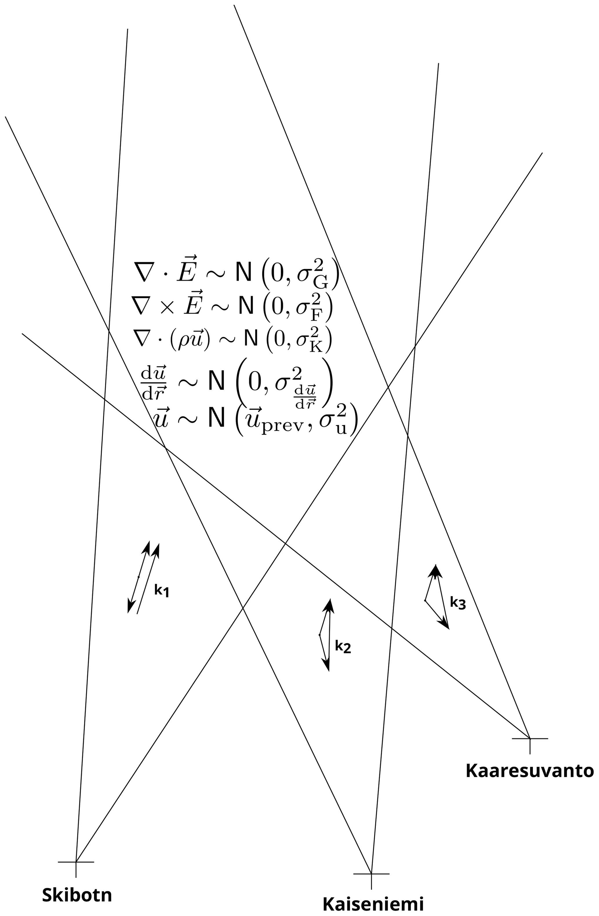
Figure 1 The figure shows geometry and assumptions on E3D volumetric measurements. The figure is not to scale or angle.

The relationship between a measurement of the Doppler shift w and the ion velocity vector v for a transmitter–receiver pair p is

$$\begin{array}{}\text{(1)}& w_p={\displaystyle \frac{{\mathit{k}}_p}{\left|{\mathit{k}}_p\right|}}\cdot \mathit{v}.\end{array}$$

A set of Doppler-shift measurements ${\mathit{w}}^{\top }=[w_{\mathrm{1}},\mathrm{\dots },w_P]$ of the same volume from P pairs can be combined to the system

$$\begin{array}{}\text{(2)}& \mathit{w}=\mathbf{K}\mathit{v}+{\mathit{\xi }}_w,\end{array}$$

where ${\mathbf{K}}^{\top }=\left[{\mathit{k}}_{\mathrm{1}}/\left|{\mathit{k}}_{\mathrm{1}}\right|,\mathrm{\dots },{\mathit{k}}_P/\left|{\mathit{k}}_P\right|\right]$ is the theory matrix and ξ_w is a vector containing the noise terms. If the measurements are sufficiently linearly independent, the ion velocity can be found with the method of least squares (see Aster et al., 2013; Risbeth and Williams, 1985).

Ion velocity is determined by the ion momentum equation:

$$\begin{array}{}\text{(3)}& \begin{array}{rl}{n}_{\mathrm{i}}{m}_{\mathrm{i}}{\displaystyle \frac{\mathrm{d}\mathit{v}}{\mathrm{d}t}}& =-\mathrm{\nabla }{\mathbb{P}}_{\mathrm{i}}+n_{\mathrm{i}}{m}_{\mathrm{i}}\mathit{g}+q_{\mathrm{i}}{n}_{\mathrm{i}}\left(\mathit{E}+\mathit{v}\times \mathit{B}\right)\\ & -\sum _k{n}_{\mathrm{i}}{m}_{\mathrm{i}}{\mathit{\nu }}_{\mathrm{i}k}\left(\mathit{v}-{\mathit{v}}_k\right).\end{array}\end{array}$$

In the equation, n_i is the ion mass, m_i is the average mass of ions, ℙ_i is the pressure tensor for ions, g is the gravitational acceleration, q_i is the ion charge, E is the electric field vector, B is the magnetic field, ν_ik is the momentum-transfer collision frequency between ions and particle species k, and v_k is the velocity of particle species k. At ionospheric altitudes, the dominant terms are the Lorentz force and collision with neutrals. Gravity and pressure gradients may influence the ions from the upper E region and upwards. The gravity force is constant and the pressure can be included when we have actual measurements. For the sake of clarity and without loss of generality, we can simplify the problem by neglecting these terms. We assume singly charged ions q_i=q_e, plasma quasi-neutrality n_i=n_e and only consider collisions with neutrals. When also assuming steady-state conditions, the ion momentum equation can be written as

$$\begin{array}{}\text{(4)}& \mathrm{0}=q_{\mathrm{e}}{n}_{\mathrm{e}}\left(\mathit{E}+\mathit{v}\times \mathit{B}\right)-n_{\mathrm{e}}{m}_{\mathrm{i}}{\mathit{\nu }}_{\mathrm{in}}\left(\mathit{v}-\mathit{u}\right).\end{array}$$

To simplify the algebra, we rewrite the cross product with a matrix multiplication. We introduce the matrix:

$$\begin{array}{}\text{(5)}& {\mathbf{B}}_{\mathrm{g}}=\left[\begin{array}{ccc}\mathrm{0}& B_z& -B_y\\ -B_z& \mathrm{0}& B_x\\ B_y& -B_x& \mathrm{0}\end{array}\right],\end{array}$$

where x,y and z are the axes of the geographic coordinate system, i.e., east, north and up, respectively. This allows us to rewrite the cross product as $\mathit{v}\times \mathit{B}={\mathbf{B}}_{\mathrm{g}}{\mathit{v}}_{\mathrm{g}}$, where the subscript g shows that the matrix and vector are in geographic coordinates. Now, the momentum equation can be rewritten as

$$\begin{array}{}\text{(6)}& \left(\mathbf{I}-{\displaystyle \frac{\mathit{\kappa }}{B}}{\mathbf{B}}_{\mathrm{g}}\right){\mathit{v}}_{\mathrm{g}}={\displaystyle \frac{\mathit{\kappa }}{B}}{\mathit{E}}_{\mathrm{g}}+{\mathit{u}}_{\mathrm{g}},\end{array}$$

where

$$\begin{array}{}\text{(7)}& \mathit{\kappa }={\displaystyle \frac{q_{\mathrm{e}}B}{m_{\mathrm{i}}{\mathit{\nu }}_{\mathrm{in}}}}\end{array}$$

is the ion mobility and I is the identity matrix. Inverting the matrix on the left-hand side is simplified by transforming it into local magnetic coordinates perpendicular to the magnetic field towards the east and antiparallel. The third component completes the right-handed system and will be referred to as northward. The transformation matrix from local geomagnetic to geographic coordinates is

$$\begin{array}{}\text{(8)}& \mathbf{R}=\left[\begin{array}{ccc}\cos \mathit{\delta }& \sin I\sin \mathit{\delta }& -\cos I\sin \mathit{\delta }\\ -\sin \mathit{\delta }& \sin I\cos \mathit{\delta }& \cos I\cos \mathit{\delta }\\ \mathrm{0}& \cos I& \sin I\end{array}\right],\end{array}$$

where δ is declination and I is the magnetic dip angle (Heinselman and Nicolls, 2008). The matrix R is a rotation matrix, which means that ${\mathbf{R}}^{-\mathrm{1}}={\mathbf{R}}^{\top }$. The matrix on the left-hand side of Eq. (6) can then be written as ${\mathbf{RC}}_{\mathrm{m}}^{-\mathrm{1}}{\mathbf{R}}^{\top }$, where

$$\begin{array}{}\text{(9)}& {\mathbf{C}}_{\mathrm{m}}={\displaystyle \frac{\mathrm{1}}{\mathrm{1}+{\mathit{\kappa }}^{\mathrm{2}}}}\left[\begin{array}{ccc}\mathrm{1}& -\mathit{\kappa }& \mathrm{0}\\ \mathit{\kappa }& \mathrm{1}& \mathrm{0}\\ \mathrm{0}& \mathrm{0}& \mathrm{1}+{\mathit{\kappa }}^{\mathrm{2}}\end{array}\right].\end{array}$$

The momentum equation can now be written as

$$\begin{array}{}\text{(10)}& {\mathit{v}}_{\mathrm{g}}={\mathbf{R}}^{\top }{\mathbf{C}}_{\mathrm{m}}\mathbf{R}{\mathit{u}}_{\mathrm{g}}+{\displaystyle \frac{\mathit{\kappa }}{B}}{\mathbf{R}}^{\top }{\mathbf{C}}_{\mathrm{m}}{\mathit{E}}_{\mathrm{m}},\end{array}$$

indicating that we will estimate the electric field in local magnetic coordinates.

3 Vector field estimation model and grid

This section defines the model that will be used to estimate electric field and neutral wind from multi-beam multistatic ISR observations of ion velocity. The electric field and neutral wind each have three components which have to be found from a discrete set of three components of ion wind. This gives six unknowns for three measurements. In addition to relating the ion velocity with the electric field and neutral wind, constraints are therefore also applied to find a more stable solution.

The discretization of the problem should keep most of its important features. The volume unknown is represented by discrete basis functions where we use a discretization corresponding to boxcars (voxels) in a desired coordinate system. This simplifies the search for discretization to find one coordinate system for each unknown. It is an advantage for computation speed to let the discretization be as coarse as possible because fewer parameters have to be estimated.

The electric field is strongly affected by the electric conductivities. This means that the fields are stronger in directions where the conductivity is low. Since the conductivity is much higher along the magnetic field than perpendicular to it (Brekke, 2013), electric fields and their variations are expected to mainly be in the perpendicular direction for higher altitudes. To avoid aliasing-type problems, it is preferable to use a discretization that is aligned with the magnetic field.

The neutral wind is expected to vary predominantly perpendicular to gravity and therefore following the surface of Earth. A geographic-oriented coordinate system is therefore an advantage for the neutral wind.

This means that the preferred coordinate systems for the discretization of electric field and neutral wind are different. We now introduce the discretization. We start with the measurements of the ion velocity. Here, for measurement ℓ, the measured ion velocity υ_ℓ is considered as an integral over the probed volume indicated with the function β_ℓ. The measurement can be written as

$$\begin{array}{}\text{(11)}& {\mathit{\upsilon }}_{\mathrm{\ell }}=\underset{V}{\iiint }\mathit{v}\left(\mathit{r}\right){\mathit{\beta }}_{\mathrm{\ell }}\left(\mathit{r}\right)\mathrm{d}V+{\mathit{\xi }}_{\mathrm{\ell }},\end{array}$$

where ξ_ℓ is a vector which contains the errors of the ion velocity vector measurements, i.e., the errors of the solution of Eq. (2). Equation (11) can be expanded using the momentum equation, Eq. (10). This gives

$$\begin{array}{}\text{(12)}& \begin{array}{rl}{\mathit{\upsilon }}_{\mathrm{\ell }}& =\underset{V}{\iiint }{\mathbf{R}}^{\top }{\mathbf{C}}_{\mathrm{m}}\mathbf{R}{\mathit{u}}_{\mathrm{g}}\left(\mathit{r}\right)\left|\det {\mathbf{J}}_u\right|{\mathit{\beta }}_{\mathrm{\ell }}\left(\mathit{r}\right)\mathrm{d}V\\ & +\underset{V}{\iiint }{\displaystyle \frac{\mathit{\kappa }}{B}}{\mathbf{R}}^{\top }{\mathbf{C}}_{\mathrm{m}}{\mathit{E}}_{\mathrm{m}}\left|\det {\mathbf{J}}_E\right|{\mathit{\beta }}_{\mathrm{\ell }}\left(\mathit{r}\right)\mathrm{d}V+{\mathit{\xi }}_{\mathrm{\ell }},\end{array}\end{array}$$

where J is the Jacobian from the coordinate system of the ion velocity to that one indicated by the subscript, u for neutral wind and E for electric field. Then, the unknown continuous vector fields are discretized by replacing them with sums of basis functions Φ_j and Ψ_j:

$$\begin{array}{}\text{(13)}& E_x\approx \sum _{j=\mathrm{1}}^{N_E}{\mathit{\eta }}_{jx}{\mathrm{\Phi }}_{jx}\end{array}$$

and

$$\begin{array}{}\text{(14)}& u_x\approx \sum _{j=\mathrm{1}}^{N_u}{\mathrm{\Gamma }}_{jx}{\mathrm{\Psi }}_{jx},\end{array}$$

and correspondingly for the other dimensions.

This converts the continuous vector field to a discrete form where the coefficients η_j and Γ_j are our new set of unknowns. They are constant over the integrated volume and can therefore be taken out of the integral. We will now define the variables

$$\begin{array}{}\text{(15)}& a_{\mathrm{\ell }j}^E=\underset{V}{\iiint }{\displaystyle \frac{\mathit{\kappa }}{B}}{\mathbf{R}}^{\top }{\mathbf{C}}_{\mathrm{m}}{\mathbf{\Phi }}_j\left|\det {\mathbf{J}}_E\right|{\mathit{\beta }}_{\mathrm{\ell }}\left(\mathit{r}\right)\mathrm{d}V\end{array}$$

and

$$\begin{array}{}\text{(16)}& a_{\mathrm{\ell }j}^u=\underset{V}{\iiint }{\mathbf{R}}^{\top }{\mathbf{C}}_{\mathrm{m}}\mathbf{R}{\mathbf{\Psi }}_j\left|\det {\mathbf{J}}_u\right|{\mathit{\beta }}_{\mathrm{\ell }}\left(\mathit{r}\right)\mathrm{d}V.\end{array}$$

Equations (15) and (16) let us write Eq. (12) as

$$\begin{array}{}\text{(17)}& {\mathit{\upsilon }}_{\mathrm{\ell }}=\sum _{j=\mathrm{1}}^{N_u}{a}_{\mathrm{\ell }j}^u{\mathrm{\Gamma }}_j+\sum _{j=\mathrm{1}}^{N_E}{a}_{\mathrm{\ell }j}^E{\mathit{\eta }}_j+{\mathit{\xi }}_{\mathrm{\ell }},\end{array}$$

which can be recognized as a matrix equation υ = ${\mathbf{A}}_E\mathit{\eta }+{\mathbf{A}}_u\mathbf{\Gamma }+\mathit{\xi }$. If we define the unknowns as one single vector ${\mathit{x}}^{\top }=\left[{\mathrm{\Gamma }}^{\top },{\mathit{\eta }}^{\top }\right]$ and stack the matrices ${\mathbf{A}}^{\top }=\left[{\mathbf{A}}_u^{\top },{\mathbf{A}}_E^{\top }\right]$, the equation relating the measurements to the unknowns becomes

$$\begin{array}{}\text{(18)}& \mathit{\upsilon }=\mathbf{A}\mathit{x}+\mathit{\xi }.\end{array}$$

The equation can be recognized as a standard linear inverse problem for which we develop a general physics-based solution in this paper.

The nature of the problem is underdetermined as shown by the earlier works (e.g., Brekke et al., 1973; Semeter et al., 2009; Nygrén et al., 2011, 2012; Nicolls et al., 2014; Swoboda et al., 2017; Stamm et al., 2021a). We therefore have to use regularization.

The main objective of regularization is to reduce the impact of noise amplification caused by the very smallest eigenvalues of the theory matrix. This can be achieved by a range of regularizing functions. It is preferable to choose regularization that biases the solution towards some sensible properties. In this paper, we suggest forcing the solution to adhere to plasma physics conservation equations: the continuity and momentum equations as well as Maxwell's equations. This gives a physical justification for regularization. However, it is still worth keeping the regularization as weak as possible to not impact the solution too much.

Here, we will show that for the electric field and neutral wind, we can use fundamental physical laws to obtain regularization terms similar to Tikhonov regularization. The outcome is twofold: (i) it gives a less noisy solution and (ii) it forces it to be physically reasonable.

By using Gauss' law $\mathrm{\nabla }\cdot \mathit{E}=\mathrm{0}$ for a charge-neutral plasma and Faraday's law $\mathrm{\nabla }\times \mathit{E}=\mathbf{0}$ for a time-stationary magnetic field, we are adding four equations for every unknown vector of the electric field.

For the neutral wind, we use the continuity equation $\mathrm{\nabla }\cdot \left(\mathit{\rho }\mathit{u}\right)=\mathrm{0}$, where ρ is the mass density of neutral particles. Also, we assume that the acceleration of the neutral wind is small. This means that when the same particles have moved for some time, and thereby distance, they have the same velocity. Furthermore, this implies that the spatial variation of the neutral wind vector field is small. We implement this approximation by assuming that the first-order differences of the neutral wind components in all directions are smaller than some parameter 1/α. These constraints are mathematically equivalent to first-order Tikhonov regularization (Aster et al., 2013; Roininen et al., 2011).

With small neutral wind accelerations, one can also argue the use of previous neutral wind estimates as prior assumption of the next neutral wind estimate. This corresponds to a zeroth-order Tikhonov regularization and would then be similar to a Kalman filter, or to the approach introduced by (Nygrén et al., 2011).

Many of the regularization terms we introduce contain spatial derivatives in multiple dimensions at the same time. For example, each component of Faraday's law uses derivatives in two directions, as illustrated in Fig. 2. Since these derivatives are not symmetrical in this case, we use a weighting of the derivatives in both directions. They are approximated by

$$\begin{array}{}\text{(19)}& \begin{array}{rl}{\displaystyle \frac{\mathrm{d}{E}_x}{\mathrm{d}y}}\left(y\right)& \approx W_{\mathrm{1}}{\displaystyle \frac{E_x(y+\mathrm{\Delta }{y}_{\mathrm{1}})-E_x\left(y\right)}{\mathrm{\Delta }{y}_{\mathrm{1}}}}\\ & +W_{\mathrm{2}}{\displaystyle \frac{E_x\left(y\right)-E_x(y-\mathrm{\Delta }{y}_{\mathrm{2}})}{\mathrm{\Delta }{y}_{\mathrm{2}}}}\end{array}\end{array}$$

for the example of electric field in the x direction. In the equation, W₁ and W₂ are weights. We note that the separation in the grid is varying because the grid may be curved and stretched. Therefore, we have to take into account that Δy₁≠Δy₂.

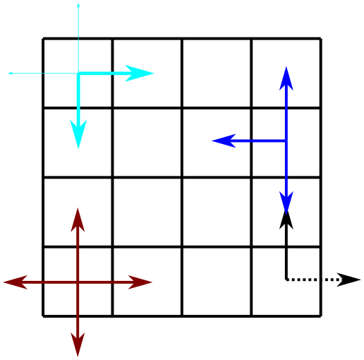
Figure 2 Problems that arise at the borders of the grid. When using the definition of the derivative, at the one side, the derivative over the border cannot be included directly (black arrows). Possible solutions to the border problem for symmetric derivatives are also shown in the figure (cyan, blue, brown arrows).

Additionally, when differentiating in different dimensions, border issues appear in some cases since the derivatives can only be found in certain directions, see Fig. 2. Mathematically, the solutions to this problem differ depending on the weights (W₁ and W₂) that are used. We are aware of three possible solutions. The first is to ignore the derivatives passing the border. Then, one of the weights is zero, which is shown as the blue line in Fig. 2.

Another possibility is to take the border-passing derivatives as stochastic variables, e.g.,

$$\begin{array}{}\text{(20)}& {\displaystyle \frac{E_x\left(y\right)-E_x(y-\mathrm{\Delta }{y}_{\mathrm{2}})}{\mathrm{\Delta }{y}_{\mathrm{2}}}}\sim N\left(\mathrm{0},{\mathit{\sigma }}_{\mathrm{\Delta }E}^{\mathrm{2}}\right).\end{array}$$

A third possibility is to weigh the two derivatives in another way, e.g., by focusing on those inside the borders. An example is illustrated by the cyan arrows in Fig. 2.

The problems described above do not apply to the 1D derivatives in the first-order Tikhonov regularization for the neutral wind. In this case, we simply use the definition of the derivative.

These regularizing constraints add several terms to our inverse problem. The physics-based regularized function we are minimizing is

$$\begin{array}{}\text{(21)}& \begin{array}{rl}& {\left(\mathit{m}-\mathbf{A}\mathit{x}\right)}^{\top }{\mathrm{\Sigma }}_{\mathrm{m}}^{-\mathrm{1}}\left(\mathit{m}-\mathbf{A}\mathit{x}\right)+{\left(\mathrm{\nabla }\times \mathit{E}\right)}^{\top }{\mathrm{\Sigma }}_{\mathrm{F}}^{-\mathrm{1}}\left(\mathrm{\nabla }\times \mathit{E}\right)\\ & +{\left(\mathrm{\nabla }\cdot \mathit{E}\right)}^{\top }{\mathrm{\Sigma }}_{\mathrm{G}}^{-\mathrm{1}}\left(\mathrm{\nabla }\cdot \mathit{E}\right)+{\left(\mathrm{\nabla }\cdot \left(\mathit{\rho }\mathit{u}\right)\right)}^{\top }{\mathrm{\Sigma }}_{\mathrm{K}}^{-\mathrm{1}}\left(\mathrm{\nabla }\cdot \left(\mathit{\rho }\mathit{u}\right)\right)\\ & +{\left({\displaystyle \frac{\mathrm{d}\mathit{u}}{\mathrm{d}\mathit{r}}}\right)}^{\top }{\mathrm{\Sigma }}_{\frac{\mathrm{d}\mathit{u}}{\mathrm{d}\mathit{r}}}^{-\mathrm{1}}\left({\displaystyle \frac{\mathrm{d}\mathit{u}}{\mathrm{d}\mathit{r}}}\right)+{\left(\mathit{u}-{\mathit{u}}_{\mathrm{prev}}\right)}^{\top }{\mathrm{\Sigma }}_{\frac{\mathrm{d}\mathit{u}}{\mathrm{d}t}}^{-\mathrm{1}}\left(\mathit{u}-{\mathit{u}}_{\mathrm{prev}}\right).\end{array}\end{array}$$

Here, the covariance matrices in the different regularization terms fulfill the same role as the regularization parameter in a standard Tikhonov regularization. They balance how tightly the solution fits the constraints relative to how well they fit the observations.

It is possible to rewrite this in matrix form as

$$\begin{array}{}\text{(22)}& {\mathit{\upsilon }}_R={\mathbf{A}}_R\mathit{x}+{\mathit{\xi }}_R,\end{array}$$

where the extended theory matrix is ${\mathbf{A}}_R^{\top }=\left[{\mathbf{A}}^{\top },{\mathbf{L}}^{\top }\right]$. Here, the matrix L is the regularization matrix which contains all the regularization terms constraining the problem.

4 Model simulation

To analyze the resolution and accuracy that the proposed estimation technique provides, we perform a simulation of the system. Here we use different grids for ion drifts, electric field and neutral wind.

For the simulated measurements, we use an experiment consisting of 5×7 beams, as illustrated in Figs. 3, 4 and 5. The beams are pointed evenly as a fan with zenith angles from 13^∘ S to 5^∘ N, with a spacing of 3^∘. In the E–W direction, we have beams every 2.5^∘ between 5^∘ W and 5^∘ E. According to the International Geomagnetic Reference Field (IGRF) model (Thébault et al., 2015), in 2022, the magnetic field at 69^∘ N, 20^∘ E has a declination of 10^∘ and an inclination of 78^∘. The beams and the magnetic field are pointed out in Fig. 5. In every beam, we measure with ranges every 5 km range resolution from 90 to 210 km range.

Figure 3 Longitude–height view of experimental layout. The radar beams are shown in blue, the grid for neutral wind in black and the grid for electric field in red.

Figure 4 Latitude–height view of experimental layout.

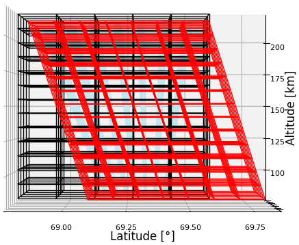
Figure 5 Azimuth–elevation distribution of transmit beams. The orange dot shows the direction of the magnetic field in 2022 as calculated with the IGRF model.

We model the measurements using a Gaussian beam pattern perpendicular to the range direction and triangular weights along the range. The vertices of the triangle are placed in the center of the next range gate. At the nearest and furthest ranges, the triangles are symmetric. The Gaussian functions are centered around the line of sight with a standard deviation of 1^∘ corresponding to the half-power beamwidth (HPBW). The Gaussian is truncated at 2 standard deviations and normalized such that it still integrates to 1.

The grid for the neutral wind uses geographic coordinates, as shown in Figs. 3 and 4. The grid centers are placed every 0.15^∘ between 68.9–69.5^∘ latitude and every 0.3^∘ between 19.8–20.7^∘ longitude. In altitude, we place the centers every 10th kilometer between 90 and 210 km.

For the electric field, we choose a special coordinate system. One axis is field-aligned and therefore slightly curved, as the magnetic field is not completely straight. However, in a short height range, as in Figs. 3 and 4, the curvature is not visible. The other axes consist of geographic latitude and longitude at the surface of Earth. We place the horizontal grid centers for the electric field every 0.1^∘ within 69.3–69.9^∘ in latitude and every 0.2^∘ within 20.0–21.0^∘ in longitude on the surface of Earth. The grid contains 7 voxels in latitude and 6 voxels in longitude. Along the magnetic field axis, the centers are placed every 10th kilometer between 90 and 210 km.

4.1 Uncertainties in ion velocity vectors

In this section, we will calculate the estimation uncertainties of the electric field and neutral wind for the example setup outlined in Sect. 4. In order to find the accuracy of the solution, we must first estimate the uncertainty in the measurements, i.e., in both observations and constraints. The accuracy of ion drift observations is well understood, but depends on the ionospheric conditions, primarily the electron density. Thus, the uncertainty varies over time, space and with the component considered (e.g., Stamm et al., 2021a). Some assumptions are therefore necessary. Here, we performed similar calculations to Stamm et al. (2021a) but using parameters of E3D when the full first stage is finished, i.e., a HPBW of 1^∘, transmit power of 5 MW, and transmit and receive gains of 43 dB. We also increased the averaging in range of the measurements to 4500 m in order to fit better to the setup in this study, giving a baud length of 30 µs. The interpulse period is 5 ms, which gives 4000 samples of the autocorrelation function in time. With an integration time of 2 s, the horizontal ion drift can be measured with around 20 m s⁻¹ accuracy in the horizontal and 5 m s⁻¹ in the vertical direction. This makes a full loop over all 35 beams that takes 70 s.

When we calculate the uncertainties, we have neglected the effects of cases where transmit and receive beams only overlap partially, decreased transmit/receive gains for tilted beams and scattering angles below 90^∘. All these effects will increase the uncertainty in ion drift observations, but not significantly.

4.2 Regularization parameters

The next step is to select suitable weights for the regularization terms, i.e., Maxwell's laws, the continuity equation and the assumption of low neutral wind acceleration. This can be interpreted as estimating the uncertainty in uncovered terms or the additional constraints they impose. The equations for Gauss's law are equivalent to saying that the expected ionospheric charge density is zero with a variance that corresponds to some value of $\mathit{\rho }/{\mathit{\epsilon }}_{\mathrm{0}}$, where ρ is the net charge density and ε₀ is the permittivity in vacuum. The uncertainty in the regularization of Gauss's law is thereby decided by the amount of plasma charge neutrality. We can, for example, assume that the usual deviation from charge neutrality is 1 to 1 million, meaning that for 10⁶ electrons, 1 is missing a positive charge. If the electron density is 10¹¹ m⁻³, around 10⁵ electrons do not have a corresponding positive charge. Then, the net charge in the plasma is in the size of 10⁻¹⁴ C m⁻³. In sum, we assume that $\mathrm{\nabla }\cdot \mathit{E}\sim \mathcal{N}(\mathrm{0},({\mathrm{10}}^{-\mathrm{3}}\mathrm{V}{\mathrm{m}}^{-\mathrm{2}}{)}^{\mathrm{2}})$.

In Faraday's law, the uncovered term is the time derivative of the magnetic field. In general, time variations in the magnetic field are mostly quite slow, but sometimes it changes very rapidly, for instance during substorms. To also include these conditions, we will use a rapid-changing magnetic field as a measure. For example, wave-like structures in the magnetic field with amplitude up to 100 nT and a frequency of 0.5 Hz have been observed in situ (Akbari et al., 2022). This corresponds to changes at the magnitude of 100 nT⋅ 2π⋅0.5 Hz ≈ 300 nT s⁻¹. We will therefore assume that the time-derivative of any magnetic field component is distributed as $\frac{\mathrm{d}{B}_{(x,y,z)}}{\mathrm{d}t}\sim \mathcal{N}(\mathrm{0},(\mathrm{300}\mathrm{nT}{\mathrm{s}}^{-\mathrm{1}}{)}^{\mathrm{2}})$.

The continuity equation for neutrals is

$$\begin{array}{}\text{(23)}& {\displaystyle \frac{\mathrm{d}\mathit{\rho }}{\mathrm{d}t}}+\mathrm{\nabla }\cdot \left(\mathit{\rho }\mathit{u}\right)=\mathrm{0}.\end{array}$$

We assume that the strongest changes in neutral density are caused by gravity waves. Vargas et al. (2019) did a study, investigating 45 sodium (Na) lidar measurements of gravity waves in São José dos Campos in the years between 1994 and 2004. They found that the fluctuations in Na density were around 3 %. The time between the minimum and maximum of waves was measured down to 1 h, but we will set this period to 10 min to allow for faster variations (see e.g., Kelly, 2009). At 100 km altitude, the mass density is around 10⁻⁷ kg m⁻³. We therefore assume that $\frac{\mathrm{d}\mathit{\rho }}{\mathrm{d}t}\sim \mathcal{N}(\mathrm{0},(\mathrm{5}\times {\mathrm{10}}^{-\mathrm{12}}\mathrm{kg}{\mathrm{m}}^{-\mathrm{3}}\mathrm{s}{)}^{\mathrm{2}})$.

In sum, with these variances, we assume that 67 % of the time, the net charge density in the plasma volume is lower than 10⁻¹⁴ C m⁻³, the magnetic field varies less than 300 nT s⁻¹, and the neutral mass density varies less than $\mathrm{5}\times {\mathrm{10}}^{-\mathrm{12}}$ kg (m³s)⁻¹.

In addition, we need to have some estimate for the cases where we consider the derivative of electric field or neutral wind across the edges of our grids and for the constraint of small neutral wind accelerations. We implement both of these in the same way where we let the gradient be a stochastic variable with a variance as in Eq. (20). For the electric field, we use the uncertainties that Stamm et al. (2021a) used in the field-aligned 1D case, but use them only for these boundaries in all 3 dimensions. For these, this corresponds to assuming that the standard deviation of the electric field is smaller than 20 mV m⁻¹ per 2500 m.

For the variance of the neutral wind gradients, we use approximate variations in measurements taken with a scanning Doppler imager as shown by Zou et al. (2021). Here, it appears that the latitudinal variation in the horizontal neutral wind components is mostly below 100 m s⁻¹ per degree latitude, corresponding to about 2 m s⁻¹ per 10 km. We tighten this constraint to 1 m s⁻¹ km⁻¹. In the vertical direction, we use a looser constraint of 20 m s⁻¹ km⁻¹ to allow for wind shear. This constraint of the neutral wind is applied to the whole volume and thereby corresponds directly to the first-order Tikhonov regularization.

In addition, we constrain the magnitude of neutral wind components. For the horizontal wind, we assume that the estimates follow a normal distribution of mean zero and uncertainty of 200 m s⁻¹. However, we expect that the vertical neutral wind components are somewhat smaller, and decrease the uncertainty to 100 m s⁻¹. These constraints correspond to the zeroth-order Tikhonov regularization of the neutral wind with using 0.005 and 0.01 s m⁻¹ as the regularization parameter.

4.3 Boundary problems

With these statements, we can proceed with finding the uncertainties in estimated electric field and neutral wind. The different solutions for handling the boundary problems also impose some properties of the neutral wind and electric field estimates. We did a short investigation of the different solutions as shown in Fig. 2. Except for ignoring all border-crossing non-symmetric derivatives, all solutions give results. The best of the solutions in terms of estimation accuracy is the symmetric derivative in which we ignore those passing boundaries. When including them as stochastic variables, the uncertainty is increased. This might be the most correct way of doing it, but further on we will ignore the boundary-passing derivatives because of simplicity, i.e., we are using the dark blue arrows in Fig. 2.

4.4 Accuracy of neutral wind and electric field estimates

The resulting uncertainties in the estimates of electric field for the coordinate system, measurements and regularization described in this section are shown in Figs. 6–8.

Figure 6 Uncertainty in electric field in local magnetic east direction.

Figure 7 Uncertainty in electric field in local magnetic north direction.

Figure 8 Uncertainty in electric field in field-aligned direction.

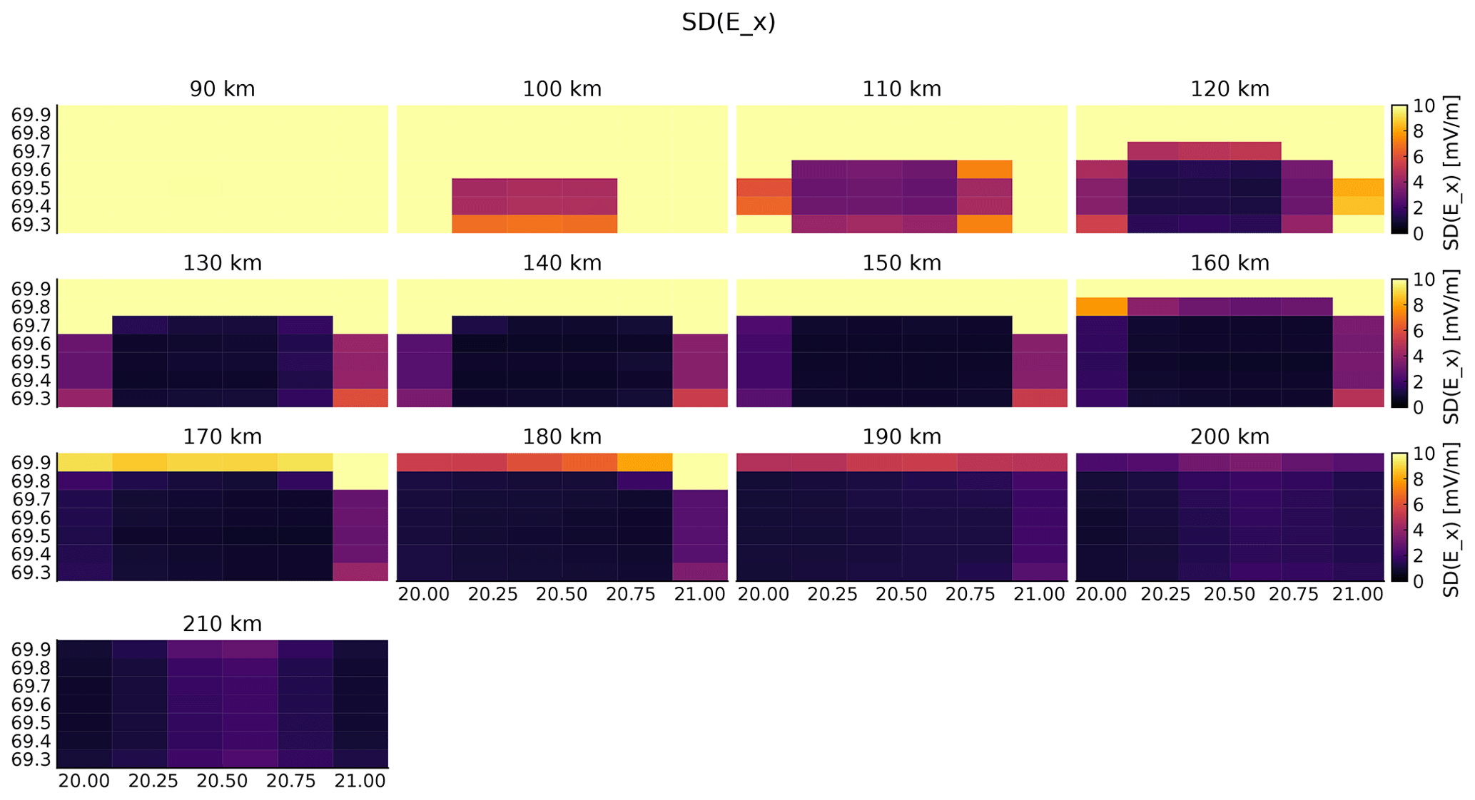
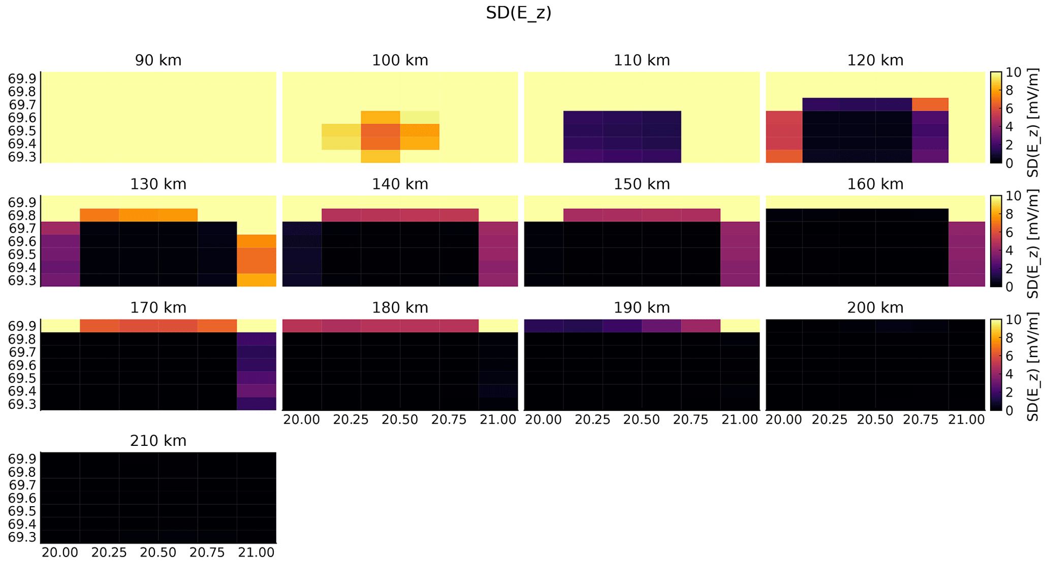
Like in the 1D case investigated by Stamm et al. (2021a), the estimates of the electric field are somewhat accurate above 125 km altitude, while being quite uncertain below 125 km. According to the figures, estimates of the electric field is possible with an accuracy in the range of a few millivolts per meter down to an altitude of 110–120 km inside the measured volume. Outside of the observed region, the electric-field uncertainties grow. This is understandable since the measurements do not include information about the electric field at those locations. There, all information comes from the constraints.

The uncertainties in neutral wind estimates are shown in Fig. 9.

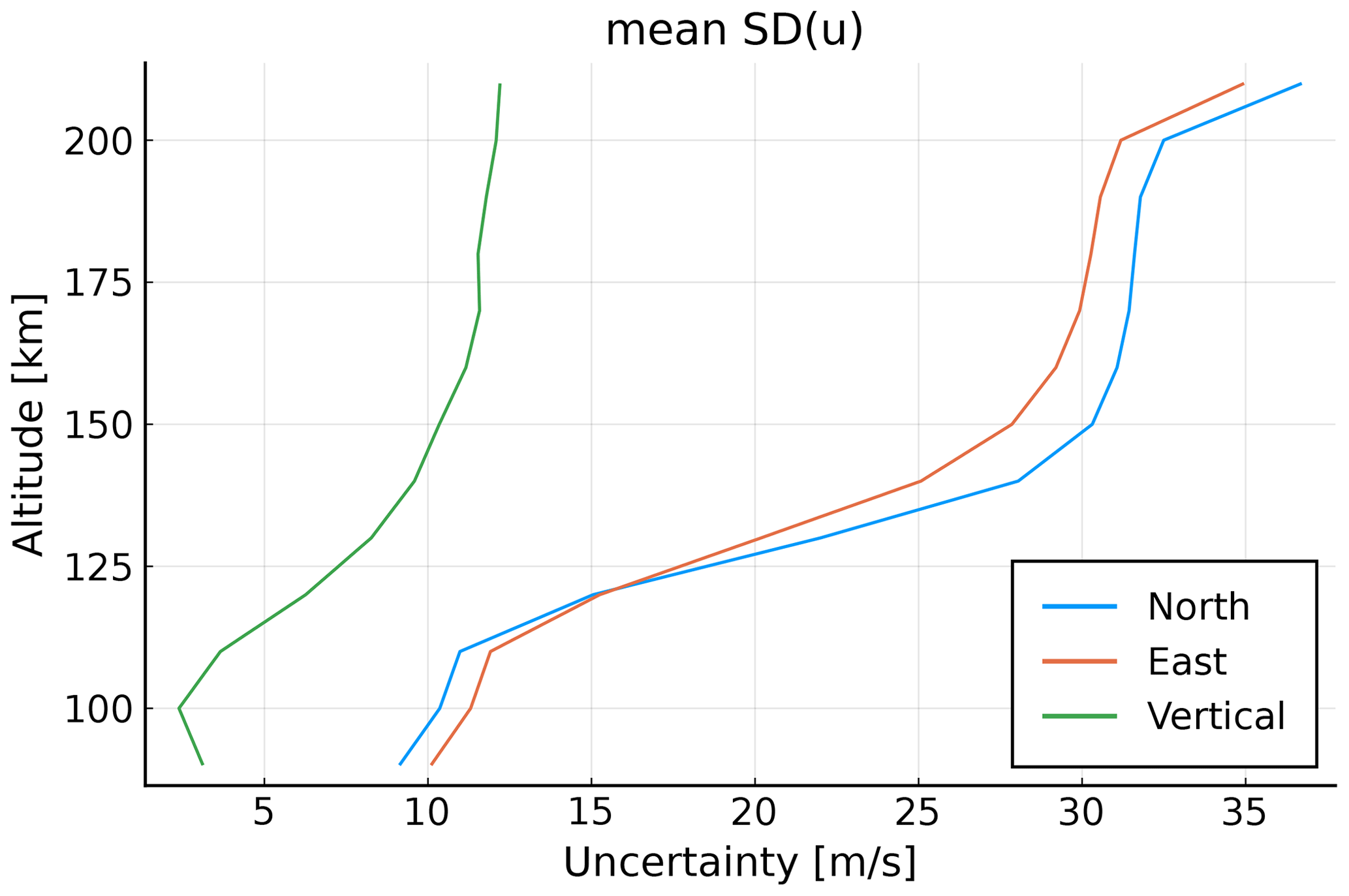
Figure 9 Uncertainty in neutral wind estimates. Because the uncertainties vary little horizontally, the values are averaged for every altitude.

The same effect is also observed here, the neutral wind can be estimated with a high accuracy at low altitudes with a variance that increases rapidly above 110 km. The lowest estimates for the neutral wind have an accuracy of lower than 20 m s⁻¹ below 120 km. These neutral wind estimates are slightly better than those for the 1D case. A reason could be our assumption that the neutral wind has little variation horizontally because then, there are more measurements (beams) measuring the “same” neutral wind volume. As in the 1D case, the accuracy of neutral wind measurements decreases with increasing altitude. It also seems to end at around the same value, namely 50 m s⁻¹.

5 Simulation results

In order to illustrate the results, we performed a vector field simulation of neutral wind and electric field. We generated a vector field where the electric field in the N–S direction points inward to a certain latitude, thereby simulating an auroral arc, similar to Nicolls et al. (2014). Inside the arc, the field is zero. Also the other components of the electric field are set to zero. This can be compared to the Cowling channel model by Fuiji et al. (2012). The neutral wind is set to zero everywhere.

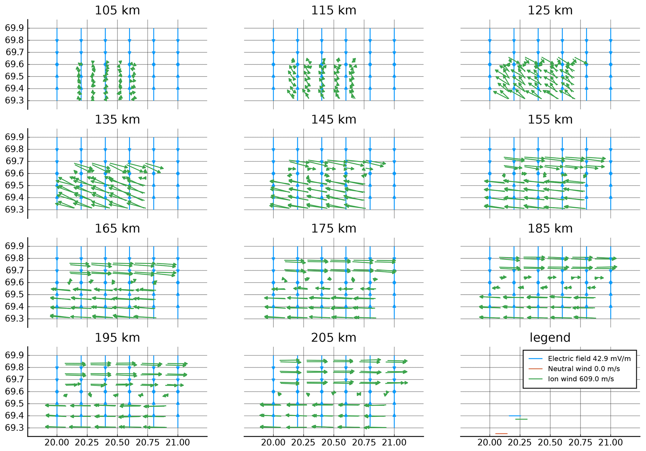
Figure 10 Electric field (blue) and neutral wind (red) used for simulations. Simulated ion wind measurements (green) are also shown. Because the neutral wind is set to zero, it is not seen in the plot. The vertical spacing in the plot is chosen so that the first plot covers our model and measurements between the 100 and 110 km range along the magnetic field, the second between 110 and 120 km, and so on. Since there are measurements every 5 km, each subplot contains two sets of measurements. For example, the 105 km plot contains the measurements from the line-of-sight ranges of 100 and 105 km. The plots for the uppermost and lowermost ranges look similar to their neighboring range and are not plotted.

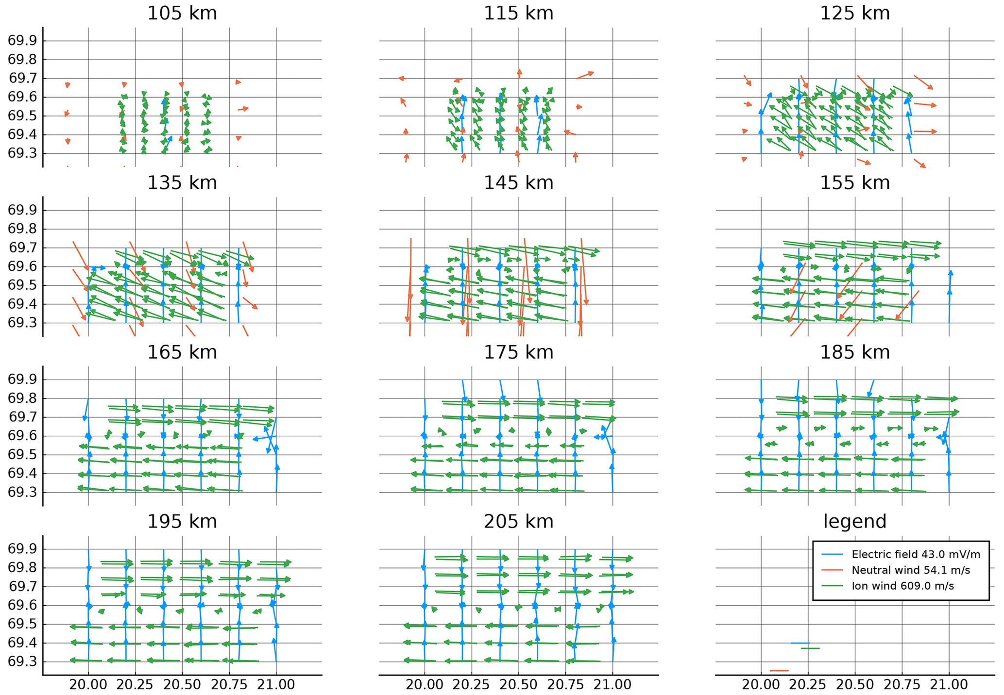
Figure 11 Estimated neutral wind (blue) and electric field (red) together with ion wind measurements (green). The plots for the uppermost and lowermost ranges look similar to their neighboring range and are not plotted. Electric field vectors where at least one component has an uncertainty larger than 10 mV m⁻¹ are not shown. Likewise, neutral wind vectors are not shown if one component has an uncertainty larger than 30 m s⁻¹.

We used the generated fields to simulate the ion velocities in the coordinate system example described in Sect. 4. Then, normally distributed noise is added with a standard deviation of 20 m s⁻¹ in the horizontal direction and 5 m s⁻¹ in the vertical direction. Finally, the simulated ion velocities are used to find estimates of neutral wind and electric field. Here, we use the same grids as for the generated fields and the regularizations as described in Sect. 4.1.

The generated vector fields for electric field and neutral wind are shown in Fig. 10 along with the ion wind measurements simulated from these. The estimated vector fields are shown in Fig. 11. The estimates where the uncertainty in at least one electric field component is above 10 mV m⁻¹, are not plotted, neither are those of neutral wind where at least one component has uncertainty above 30 m s⁻¹.

First of all, we note that the simulated ion velocity at the highest altitudes is perpendicular to the generated electric field. This is expected because at these altitudes, it is mainly influenced by the E×B drift which was used by Brekke et al. (1973) to find electric field estimates. At lower altitudes, the ion drift becomes increasingly more dependent on the neutral wind.

The shown estimate of the electric field in Fig. 11 is quite close to the starting point at 125 km and upwards, but only inside the measured volume. This is the same result as found in the one-dimensional case by Stamm et al. (2021a). We note that in the eastern boundary region of Fig. 11, there is a small curving artifact that is caused by Faraday's law.

Moreover, the neutral wind estimates can be described as somewhat correct below 125 km altitude. Those estimates above this become increasingly worse, as in the 1D study.

6 Discussion and summary

This study introduces a method to estimate electric fields and neutral winds from multistatic multi-beam ISR measurements of ion velocity. We show that electric field uncertainties of a few millivolts per meter can be achieved at altitudes above 120 km. Estimation uncertainties of neutral wind should be small below 120 km. It is the extension into 3D that marks the difference between this study and Stamm et al. (2021a). The estimates from this 3D technique give a more stable solution than in the 1D case. Even if the study is more sophisticated in 3D, the approaches give similar results which depend on how the regularization is performed. In both cases, the results indicate that even with adding regularization, electric field and neutral wind cannot be estimated well at the same altitudes without further assumptions.

For the presented estimates from the simulated ion drifts, the advantage of using the previous neutral wind estimate is not used. By using the previous neutral wind estimates as a prior knowledge of the state of the neutral wind, the time-variation of the neutral wind estimates will be smoothed. This is similar to a Kalman-filtering approach. This approach allows us to take into account that the neutral wind changes slowly with time.

The inverse problem in this study contains a number of regularization parameters that can be adjusted. When possible, we have tried to use weights for the regularization terms taken from measurements of related parameters. Elsewhere, physical models or reasoning were used.

The uncertainty in Gauss's law (10⁻³ V m⁻²) is a very large value. A stricter value can be found by considering the current continuity equation from Clayton et al. (2021) and ignoring the conductance gradients. Then,

$$\begin{array}{}\text{(24)}& {\mathrm{\nabla }}_{⟂}\cdot \mathit{E}\approx {\displaystyle \frac{{\mathit{J}}_{\parallel }}{{\mathrm{\Sigma }}_{\mathrm{P}}}},\end{array}$$

where J_∥ is the field-aligned current density and Σ_P is the Pedersen conductivity. If one assumes a field-aligned current density of $\mathrm{5}\times {\mathrm{10}}^{-\mathrm{5}}$ A m⁻² and a Pedersen conductivity of 5 Ω⁻¹ and that field-aligned variation is small, the allowed divergence of electric field decreases with some orders of magnitude. Considering the variability around dynamic auroral arcs (Dahlgren et al., 2011), we do not want to use stricter regularizations than necessary. In our model tests, it appears that the used regularization is strict enough.

However, the ideal set of regularization parameters will have to be adjusted to the real observations on a per-case basis, at least initially.

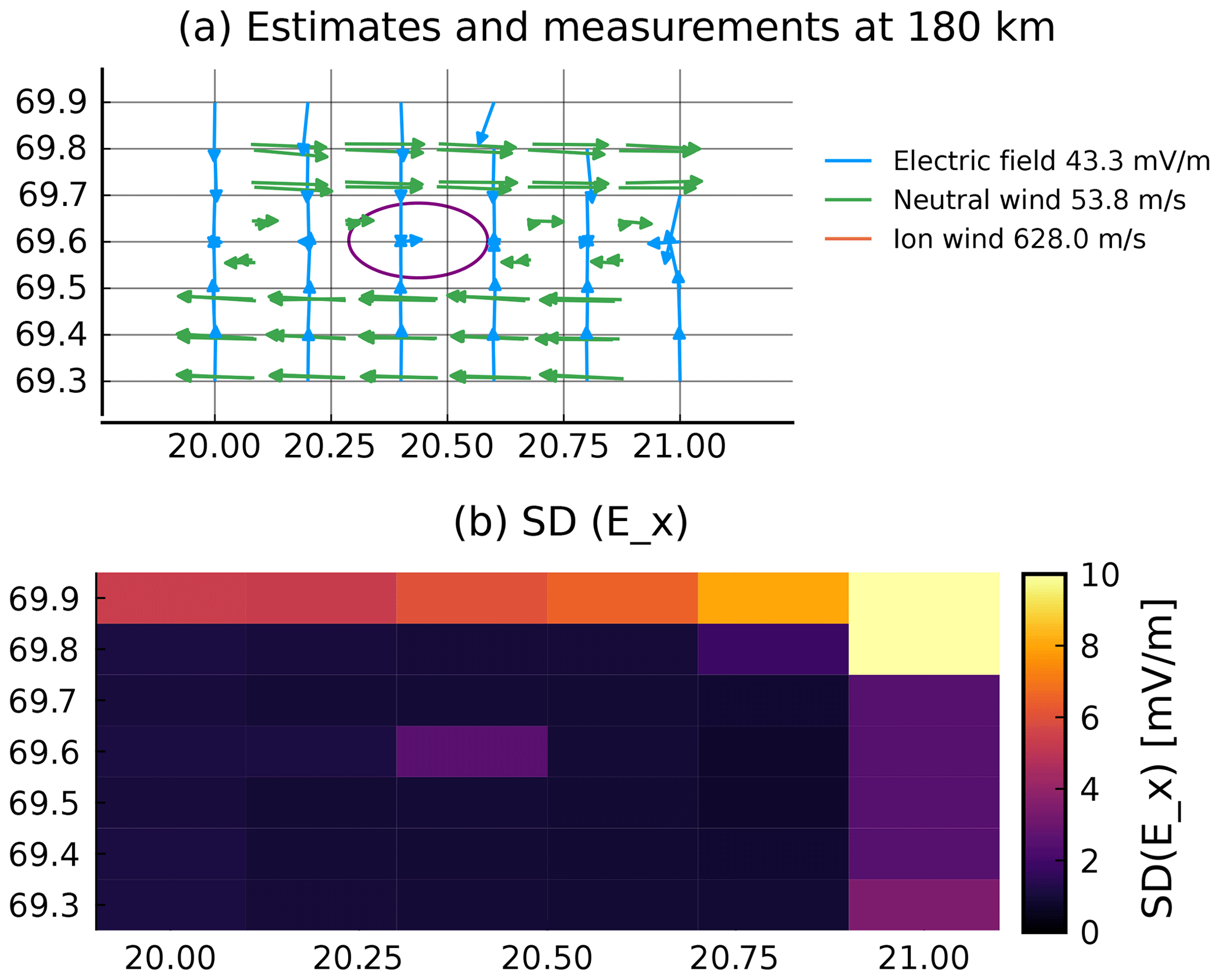
Figure 12 Estimates of electric field with measurement gap. Three central measurement beams have been removed. Panel (a) shows the remaining measurements and new estimates of electric field between 180 and 190 km. At other altitudes, the estimates show similar changes compared to Fig. 11. Panel (b) shows the corresponding uncertainties in “northward” electric field. At other altitudes, these show similar changes compared to Fig. 6.

As a performance test of the technique, we removed three of the central measurement beams and estimated electric field and neutral wind from the remaining measurements. The estimates with measurements between 180 and 190 km altitude are shown in Fig. 12a, and the E_x uncertainties in Fig. 12b. The deviations relative to the estimates using the full set of measurements (see Fig. 11) are small. Maybe more importantly, the uncertainties do not increase by much. This shows that this type of Tikhonov regularization leads to solutions that degrade gracefully while satisfying Maxwell's equations. A consequence of this is that it should be possible to use sparser beams to estimate electric field and neutral wind. This can be used to either improve the time resolution or to expand the observed volume. However, the removal of beams comes with a cost of slightly increased uncertainties, which can be seen by comparing Figs. 12b and 6.

The presented framework assumes that the ionosphere does not change faster than the integration time, which is 70 s for the presented example. Spatial and temporal variations occurring faster than the integration time will thus be blurred out. One way to mitigate this is to take into account the direction in which the beam points at every point in time, such that the model connects the time the measurement is taken to the results. Another possible mitigation procedure is to use a shorter integration time. The latter will have increased uncertainty which may be compensated by a Kalman filter to some extent. A third option would be to use fewer beams as this needs shorter integration time. The regularization will then try to fill the gaps as best as possible as illustrated in the example above.