Drivers of rapid geomagnetic variations at high latitudes

We have examined the most intense external (magnetospheric and ionospheric) and internal (induced) $|\mathrm{d}\mathit{H}/\mathrm{d}t|$ (amplitude of the 10 s time derivative of the horizontal geomagnetic field) events observed by the high-latitude International Monitor for Auroral Geomagnetic Effects (IMAGE) magnetometers between 1994 and 2018. While the most intense external $|\mathrm{d}\mathit{H}/\mathrm{d}t|$ events at adjacent stations typically occurred simultaneously, the most intense internal (and total) $|\mathrm{d}\mathit{H}/\mathrm{d}t|$ events were more scattered in time, most likely due to the complexity of induction in the conducting ground. The most intense external $|\mathrm{d}\mathit{H}/\mathrm{d}t|$ events occurred during geomagnetic storms, among which the Halloween storm in October 2003 featured prominently, and drove intense geomagnetically induced currents (GICs). Events in the prenoon local time sector were associated with sudden commencements (SCs) and pulsations, and the most intense $|\mathrm{d}\mathit{H}/\mathrm{d}t|$ values were driven by abrupt changes in the eastward electrojet due to solar wind dynamic pressure increase or decrease. Events in the premidnight and dawn local time sectors were associated with substorm activity, and the most intense $|\mathrm{d}\mathit{H}/\mathrm{d}t|$ values were driven by abrupt changes in the westward electrojet, such as weakening and poleward retreat (premidnight) or undulation (dawn). Despite being associated with various event types and occurring at different local time sectors, there were common features among the drivers of most intense external $|\mathrm{d}\mathit{H}/\mathrm{d}t|$ values: preexisting intense ionospheric currents (SC events were an exception) that were abruptly modified by sudden changes in the magnetospheric magnetic field configuration. Our results contribute towards the ultimate goal of reliable forecasts of $\mathrm{d}\mathit{H}/\mathrm{d}t$ and GICs.

1 Introduction

Geomagnetically induced currents (GICs) in technological conductor networks occur commonly during space weather events and have the potential to affect the performance of critical ground infrastructure such as electric power transmission grids. The amplitude of the time derivative of the horizontal ground magnetic field ($|\mathrm{d}\mathit{H}/\mathrm{d}t|$) has often been used as a proxy for the geoelectric field and GIC risk (Viljanen, 1998; Viljanen et al., 2001). Intense $|\mathrm{d}\mathit{H}/\mathrm{d}t|$ and GIC are typically attributed to substorms, sudden commencements (SCs), and geomagnetic pulsations (Viljanen et al., 1999; Rogers et al., 2020; Clilverd et al., 2021) associated with geomagnetic storms driven by interplanetary coronal mass ejections (ICMEs) and their sheaths (Huttunen et al., 2008; Kataoka and Pulkkinen, 2008). Energy input from the solar wind into the magnetosphere can be characterized by various parameters, such as the solar wind electric field or southward component of the interplanetary magnetic field (IMF), and has been found to correlate with GIC amplitudes and nightside magnetic perturbation activity (Huttunen et al., 2008; Engebretson et al., 2021). Recently, Hajra (2022) has shown that intense GICs do not occur as individual peaks but as clusters with a duration of ∼ 5–38 h associated with intense substorm clusters, characterized by a peak SuperMAG auroral electrojet index > 2000 nT.

The SC signature is a sudden increase of the horizontal geomagnetic field. It occurs when an abrupt increase in the solar wind dynamic pressure, at an interplanetary shock, for example, compresses the magnetosphere, leading to an intensification of the electric currents in the magnetosphere and ionosphere (Oliveira and Samsonov, 2018). Ultra-low-frequency (ULF) waves, which are detected on the ground as geomagnetic pulsations, are a known source of intense $|\mathrm{d}\mathit{H}/\mathrm{d}t|$. ULF waves in the magnetosphere can be caused either externally by solar wind perturbations or internally inside the magnetosphere. The most important sources of ULF waves directly driven by the solar wind are thought to be the Kelvin–Helmholtz instability and solar wind dynamic pressure pulses. Because the Kelvin–Helmholtz instability requires a shear flow, it mainly occurs at the dawn and dusk flanks of the magnetopause, especially when the solar wind speed is high (Engebretson et al., 1998).

Whereas SCs and some pulsation types can be considered to be directly driven by the solar wind, substorms are a delayed response to energy input from the solar wind into the magnetosphere. Intense $|\mathrm{d}\mathit{H}/\mathrm{d}t|$ (exceeding 1 nT s⁻¹) occurs typically during events governed by westward ionospheric currents (Viljanen et al., 2001), often during substorm onsets when the amplitude of the westward electrojet (WEJ) increases rapidly (Viljanen et al., 2006b). Juusola et al. (2015a) have shown that the temporal development of $|\mathrm{d}\mathit{H}/\mathrm{d}t|$ activity during substorms follows that of substorm currents and aurora, typically spreading from a premidnight onset region poleward, equatorward, and toward the morning sector along the auroral oval and WEJ. According to Viljanen et al. (2001) and Juusola et al. (2020), the directional distribution of intense external $\mathrm{d}\mathit{H}/\mathrm{d}t$ varies as a function of magnetic local time (MLT), developing from the predominantly north–south orientation in the premidnight sector to east–west orientation in the 02:00–05:00 MLT sector and back to north–south direction in the pre-noon sector. This change is strongest at stations at the latitudes of the nominal auroral oval and becomes weaker towards north and south, where $\mathrm{d}\mathit{H}/\mathrm{d}t$ prefers north–south orientation, even in the morning sector. According to Schillings et al. (2022), rapid “$\mathrm{d}B/\mathrm{d}t$” spikes initially occur in the premidnight sector and later spread towards the morning sector. Such a sequence is correlated with the auroral electrojet (AE) index and can repeat several times throughout a geomagnetic storm.

Intense $|\mathrm{d}\mathit{H}/\mathrm{d}t|$ events are concentrated in the pre-midnight and dawn MLT sectors (Juusola et al., 2015b; Schillings et al., 2022). The pre-midnight events are most likely associated with substorm onset. Substorm onsets leading to clear bulge-type substorms typically occur around 23:00 MLT, but they are generally not observed after 03:00 MLT (e.g., Frey et al., 2004). Auroral streamers, driven by fast magnetospheric flows, can also occur in the morning sector auroral oval (e.g., Forsyth et al., 2020). In the ground magnetic field, auroral streamers typically correspond to southward-propagating enhancements of northwestward or westward ionospheric equivalent current (Juusola et al., 2009). Streamers appear to play a role in the formation of auroral omega bands (Weygand et al., 2015; Forsyth et al., 2020; Weygand et al., 2022). Omega bands tend to be associated with times of greater than average geomagnetic activity and their occurrence peaks in the 02:00–04:00 MLT sector, mainly during substorm recovery phases (Partamies et al., 2017). The main source of magnetic disturbances on the ground during omega bands is an undulating WEJ (Opgenoorth et al., 1983), which causes $\mathrm{d}\mathit{H}/\mathrm{d}t$ in the east–west direction, although the ambient field is generally southward. Geomagnetic pulsations at periods 5–40 min, called the Ps6 category (Jacobs et al., 1964), due to the undulating WEJ are associated with omega band activity (Opgenoorth et al., 1983). Omega bands have been shown to cause intense GICs (Apatenkov et al., 2020).

Pulkkinen et al. (2003a) and Dimmock et al. (2019) have suggested that GICs are primarily driven by small-scale spatiotemporal structures superimposed on the large-scale WEJ. Recent studies have demonstrated that nighttime magnetic perturbations at high latitudes can occur in association with a range of ionospheric current systems, geomagnetic conditions, and auroral structures and can cover large, moving regions with diameters of hundreds of kilometers (Ngwira et al., 2018; Engebretson et al., 2019a, b; Dimmock et al., 2020; Weygand et al., 2021).

In this study, we will examine five events in detail with the most intense external (due to ionospheric and magnetospheric currents) $|\mathrm{d}\mathit{H}/\mathrm{d}t|$ (10 s time resolution) observed by the International Monitor for Auroral Geomagnetic Effects (IMAGE) magnetometer network between 1994 and 2018. The open question we try to approach is the details and drivers in the various processes (SCs, substorms, and pulsations) that produce the most intense $|\mathrm{d}\mathit{H}/\mathrm{d}t|$. The structure of the study is as follows: the data and methods are presented in Sect. 2, and the results are presented in Sect. 3 and discussed in Sect. 4. The conclusions are summarized in Sect. 5.

2 Data and method

2.1 Data

We have used 10 s ground magnetic field measurements from IMAGE (https://space.fmi.fi/image/, last access: 22 December 2022) magnetometers between 1994 and 2018. In 2018, IMAGE consisted of 41 stations that covered magnetic latitudes from the subauroral 47^∘ N to the polar 75^∘ N in an approximately 2 h magnetic local time (MLT) sector.

IMAGE data are provided in geographic coordinates, and we carry out the analysis using the same coordinate system. We use the notations ΔB_x, ΔB_y, and ΔB_z for the north, east, and down components of the variation ground magnetic field. The horizontal magnetic field vector is denoted by

$$\begin{array}{}\text{(1)}& \mathrm{\Delta }\mathit{H}=\mathrm{\Delta }{B}_x{\widehat{\mathit{e}}}_x+\mathrm{\Delta }{B}_y{\widehat{\mathit{e}}}_y\end{array}$$

and its amplitude by

$$\begin{array}{}\text{(2)}& \left|\mathrm{\Delta }\mathit{H}\right|=\sqrt{\mathrm{\Delta }{B}_x^{\mathrm{2}}+\mathrm{\Delta }{B}_y^{\mathrm{2}}}.\end{array}$$

Similarly, the time derivative vector and its amplitude are

$$\begin{array}{}\text{(3)}& \mathrm{d}\mathit{H}/\mathrm{d}t=\mathrm{d}{B}_x/\mathrm{d}t{\widehat{\mathit{e}}}_x+\mathrm{d}{B}_y/\mathrm{d}t{\widehat{\mathit{e}}}_y\end{array}$$

and

$$\begin{array}{}\text{(4)}& |\mathrm{d}\mathit{H}/\mathrm{d}t|=\sqrt{(\mathrm{d}{B}_x/\mathrm{d}t{)}^{\mathrm{2}}+(\mathrm{d}{B}_y/\mathrm{d}t{)}^{\mathrm{2}}},\end{array}$$

respectively. The measured magnetic field is a sum of the internal and external contributions, e.g.,

$$\begin{array}{}\text{(5)}& \mathrm{\Delta }{B}_x=\mathrm{\Delta }{B}_{x,\mathrm{internal}}+\mathrm{\Delta }{B}_{x,\mathrm{external}}.\end{array}$$

The time derivative is calculated as

$$\begin{array}{}\text{(6)}& \mathrm{d}{B}_x\left(t\right)/\mathrm{d}t=\left[\mathrm{\Delta }{B}_x\left(t\right)-\mathrm{\Delta }{B}_x(t-T)\right]/T,\end{array}$$

where T=10 s is the time step of the data. Although geographic coordinates are used to present the data, we have occasionally marked magnetic coordinates in the plots. We have used the quasi-dipole (QD) coordinates (Richmond, 1995; Emmert et al., 2010) as given by the software available at https://apexpy.readthedocs.io/en/latest/, last access: 22 December 2022. The code uses the 12th generation International Geomagnetic Reference Field (IGRF-12; Thébault et al., 2015).

To assess the GIC effectiveness of the intense external $|\mathrm{d}\mathit{H}/\mathrm{d}t|$ events, we have used 10 s GIC recordings (https://space.fmi.fi/gic/, last access: 22 December 2022) in a Finnish natural gas pipeline close to the Mäntsälä (MAN) compressor station in southern Finland (60.6^∘ N, 25.2^∘ E) (Pulkkinen et al., 2001; Viljanen et al., 2006a). MAN is located about 40 km eastward from the IMAGE magnetometer station Nurmijärvi (NUR). The 1 min SYM-H index (Iyemori and Rao, 1996), auroral electrojet indices (AE, AL, and AU; Davis and Sugiura, 1966), and solar wind data propagated to Earth's bow shock nose were extracted from NASA/GSFC's OMNI data set through OMNIWeb (Papitashvili and King, 2020). A list of sudden commencements (SCs) (Curto et al., 2007) has been obtained from http://isgi.unistra.fr/, last access: 22 December 2022. An SC is a sharp increase in the magnetic field north component, and the SC lists are made on the basis of visual inspection of magnetograms from five low-latitude observatories.

2.2 Field separation and equivalent currents

Figure 1 illustrates the chain of processes that causes geomagnetic variations and GICs. Geomagnetic variations observed on the ground are a sum of an “external” part due to electric currents in the magnetosphere and ionosphere and an “internal” part due to telluric currents induced in the conducting ground. Both current systems are 3D, but they can be replaced by divergence-free currents on two spherical shells (e.g., Haines and Torta, 1994). These equivalent currents produce the same magnetic field at the Earth's surface as the true 3D currents. The locations of the equivalent current layers are based on physical arguments: the upper layer is at 90 km altitude, practically below all currents in space, and the lower layer is just below the Earth's surface to represent all induced currents which can flow at any depth. The two-dimensional Spherical Elementary Current System (2D SECS) method (Amm, 1997; Amm and Viljanen, 1999; Pulkkinen et al., 2003a, b; Juusola et al., 2016; Vanhamäki and Juusola, 2020; Juusola et al., 2020) is one option for deriving the divergence-free equivalent currents and separating the variation magnetic field into its external and internal parts. It is based on explicit current distributions from which the magnetic field is calculated according to the Maxwell equations. In real-life applications, availability of the measured magnetic field from a finite set of points in a limited area instead of the whole globe causes some uncertainty, as discussed by Vanhamäki and Juusola (2020). Similar issues naturally concern other methods as well, such as those based on spherical harmonics or Fourier analysis.

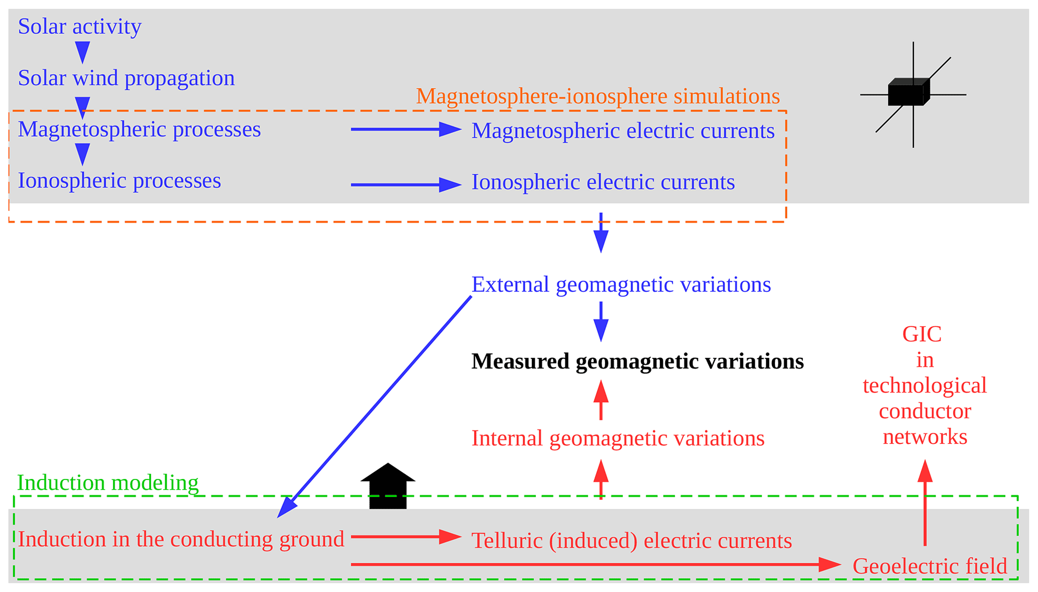
Figure 1 Principle of geomagnetic variations and geomagnetically induced currents (GICs): disturbances created by solar activity propagate to the Earth and interact with the Earth's magnetosphere–ionosphere system, creating electric currents in the near-Earth space. The spatially and temporally highly varying “external” magnetic field of these currents drives induction in the conducting ground. The “internal” magnetic field of the induced telluric electric currents is superposed to the external magnetic field, producing geomagnetic variations that can be measured by magnetometers on the ground or at low-orbit satellites. The relative contribution of internal and external magnetic fields depends on the distance of the measurement point to the various current systems, such that the internal contribution is the strongest on the ground and weakens with increasing altitude. The induced geoelectric field drives GICs in technological conductor systems. Global magnetosphere–ionosphere simulations can typically describe the external part of geomagnetic variations only, while induction modeling is needed for describing the electromagnetic interaction between the conducting Earth and external geomagnetic variations.

We have used the 2D SECS method to separate the magnetic field measured at each station into internal and external parts and to derive the external (at 90 km altitude) and internal (at 1 m depth, Juusola et al., 2016) equivalent current densities for each epoch. Before application of the 2D SECS method, a baseline needed to be subtracted from the data. Because most IMAGE stations are variometers, we could not use a model of the Earth's main field. Instead, we have used the method by van de Kamp (2013) to remove the long-term baseline (including instrument drifts), any jumps in the data, and the diurnal variation. The diurnal quiet-time magnetic field variation in the IMAGE region is at most a few tens of nanoteslas (nT) (Sillanpää et al., 2004). We concentrate on studying large time derivatives of the horizontal magnetic field for which this effect is insignificant.

Recently, Juusola et al. (2020) have shown that $|\mathrm{d}\mathit{H}/\mathrm{d}t|$ is typically dominated by the internal geomagnetic variations. Because the internal part of $|\mathrm{d}\mathit{H}/\mathrm{d}t|$ depends on the often highly structured ground conductivity (e.g., Korja et al., 2002), spatial distribution of the internal $|\mathrm{d}\mathit{H}/\mathrm{d}t|$ is more structured than that of the external $|\mathrm{d}\mathit{H}/\mathrm{d}t|$. An example that illustrates this is provided in Fig. 2.

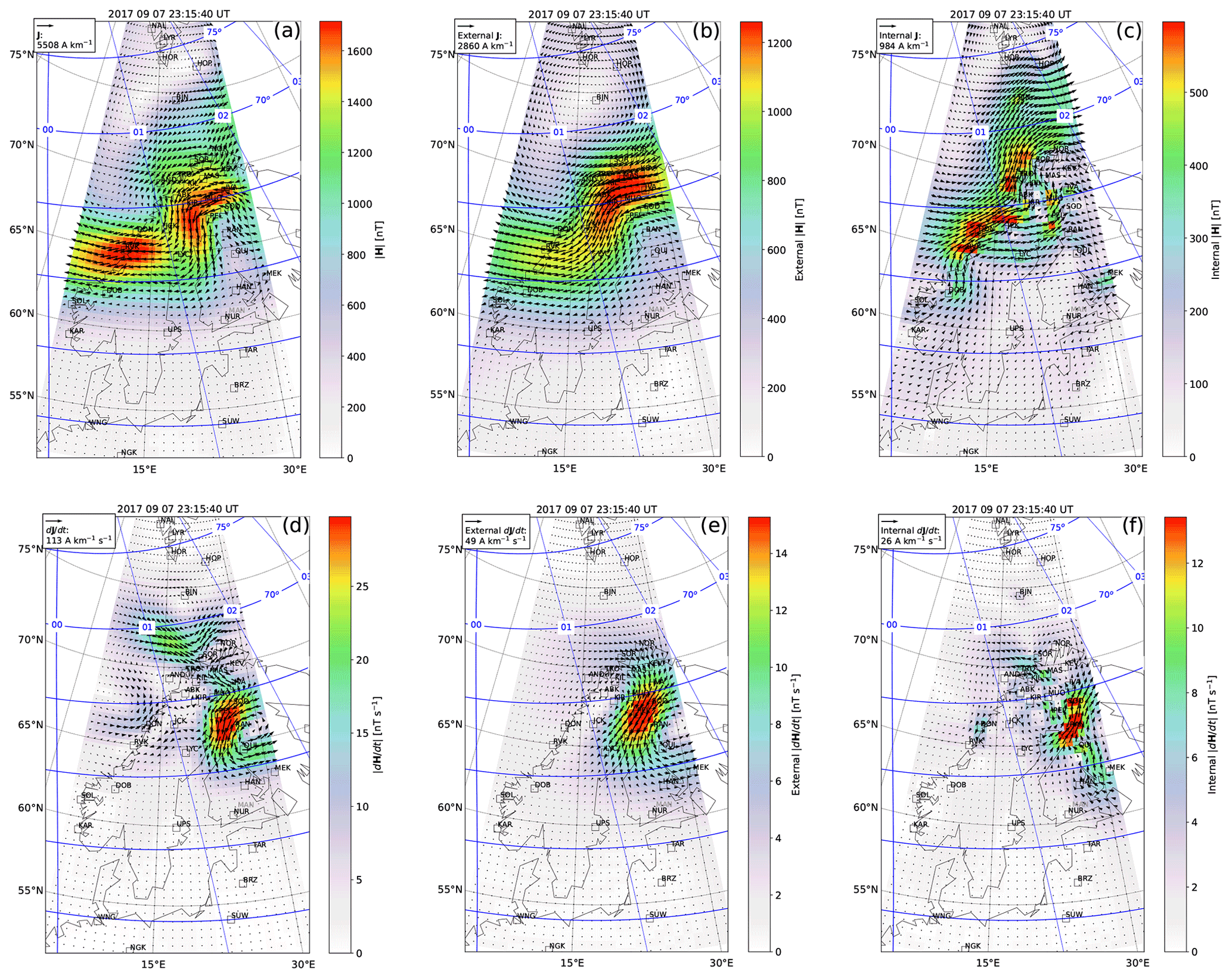
Figure 2 Effect of ground magnetic field separation: ionospheric equivalent current density (arrows) and corresponding horizontal ground magnetic field, calculated by fitting the measured ground north (ΔB_x) and east (ΔB_y) components of the geomagnetic field with a layer of 2D Spherical Elementary Current Systems (SECSs) (Vanhamäki and Juusola, 2020) at 90 km altitude (a). (b–c) Ionospheric (external) equivalent current density and corresponding ground magnetic field and induced (internal) equivalent current density and corresponding ground magnetic field, calculated by fitting the measured ΔB_x, ΔB_y, and ΔB_z with two layers of SECSs, one at 90 km altitude and the other at 1 m depth. (d–f) The same as (a)–(c) except for the time derivatives. Note that each panel has a different color and arrow length scale.

Figure 2a shows the ionospheric equivalent current density (J, arrows) and corresponding horizontal ground magnetic field magnitude ($\left|\mathrm{\Delta }\mathit{H}\right|$, color), calculated by fitting the superposed magnetic field of a layer of 2D SECSs at 90 km altitude to the measured ΔB_x and ΔB_y. ΔB_z cannot be included in the fitting because it cannot be represented in terms of ionospheric equivalent currents only (Untiedt and Baumjohann, 1993; Vanhamäki and Juusola, 2018). Fig. 2b–c show the ionospheric (external) equivalent current density and corresponding ground magnetic field and induced (internal) equivalent current density and corresponding ground magnetic field, calculated by fitting the measured ΔB_x, ΔB_y, and ΔB_z with two layers of 2D SECSs, one at 90 km altitude and the other at 1 m depth. The time derivatives corresponding to Fig. 2a–c are shown in Fig. 2d–f. Note that the color and arrow scales vary from panel to panel.

The ionospheric J and corresponding ground $\left|\mathrm{\Delta }\mathit{H}\right|$ distributions, calculated without the field separation (Fig. 2a), and particularly their time derivatives (Fig. 2d), are clearly more incoherent than those calculated with the field separation (Fig. 2b, c). In order to be able to produce the highly structured ΔH and $\mathrm{d}\mathit{H}/\mathrm{d}t$ that in reality are caused by induced currents often located close to the surface of the Earth, the ionospheric J and $\mathrm{d}\mathit{J}/\mathrm{d}t$ calculated without the field separation (Fig. 2a, d) need to have much stronger amplitudes than those calculated with the separation (Fig. 2b, e). Although no information about the ground conductivity has been used in the purely mathematical field separation, conductivity structures, such as the Norwegian coast line, are evident in the distribution of the induced J and $\left|\mathrm{\Delta }\mathit{H}\right|$ (Fig. 2c).

Without the field separation (Fig. 2a, d), the measured ΔB_x and ΔB_y are perfectly reproduced by the SECS reconstruction, but ΔB_z is not. With field separation (Fig. 2b, c, e, f), ΔB_x, ΔB_y, and ΔB_z are perfectly reproduced by the reconstruction. Note that this only applies to the magnetic field at the stations. The separation and interpolation of the geomagnetic field between the stations are not perfect and are affected by the density of the magnetometers as well as boundary conditions, as discussed by Juusola et al. (2020). Nonetheless, the internal part of the separated field has been shown to follow the known structure of the ground conductivity well (Juusola et al., 2020) (see also Fig. 2c, where the coastline is prominent), and correlation between the electrojet currents derived simultaneously from IMAGE and low-orbit satellite has been shown to significantly improve when the separation is carried out (Juusola et al., 2016). These results indicate that, although not perfect, the separation should be fairly reliable and worth carrying out.

A change in the station configuration can, under certain conditions, result in an artificial time derivative peak in the reconstructed magnetic field at the nearby stations. Because of this, we have discarded any station with data gaps during a day when processing the entire time series between 1994 and 2018 for the statistics. The time derivative has been calculated without combining values from different days. This is a fairly strict approach and wastes some usable data around midnight but ensures that there will not be any artificial time derivative peaks due to changes in station configuration.

Because induction in the ground is a complicated process, external $|\mathrm{d}\mathit{H}/\mathrm{d}t|$ may not be as good a proxy for GICs as the total $|\mathrm{d}\mathit{H}/\mathrm{d}t|$. Namely, the geoelectric field driving GICs depends significantly on local ground conductivity, the effect of which is also seen on the total $|\mathrm{d}\mathit{H}/\mathrm{d}t|$. For the same reason, studying the external $|\mathrm{d}\mathit{H}/\mathrm{d}t|$ provides more direct information on the solar wind–magnetosphere–ionosphere processes that cause intense $|\mathrm{d}\mathit{H}/\mathrm{d}t|$ values than studying the total $|\mathrm{d}\mathit{H}/\mathrm{d}t|$. Intense external $|\mathrm{d}\mathit{H}/\mathrm{d}t|$ is a requirement for strong induction and GICs, although the most intense induced $|\mathrm{d}\mathit{H}/\mathrm{d}t|$ may not occur at the same time as the most intense external $|\mathrm{d}\mathit{H}/\mathrm{d}t|$. This is because the induced current density depends on the time history of the external $\mathrm{d}\mathit{H}/\mathrm{d}t$ as well as the structure of the ground conductivity, which may favor a certain type of driving over others. Understanding the details of the solar wind–magnetosphere–ionosphere coupling that creates intense external $|\mathrm{d}\mathit{H}/\mathrm{d}t|$ is a requirement for developing our capability to forecast them. The very short persistence of the time derivative of the horizontal ground magnetic field ($\mathrm{d}\mathit{H}/\mathrm{d}t$) compared to horizontal ground magnetic field (ΔH) is a challenge for forecasting $\mathrm{d}\mathit{H}/\mathrm{d}t$ (Kellinsalmi et al., 2022). Once time series of the external ΔH with correct $\mathrm{d}\mathit{H}/\mathrm{d}t$ behavior can be predicted, fast modeling of three-dimensional (3D) induction (e.g., Marshalko et al., 2021; Kruglyakov et al., 2022) and GICs (Lehtinen and Pirjola, 1985; Viljanen et al., 2012, 2014; Kelly et al., 2017; Pirjola et al., 2022) is feasible.

3 Results

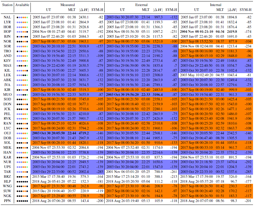
Table 1 shows the universal time (UT) of the most intense total, external, and internal $|\mathrm{d}\mathit{H}/\mathrm{d}t|$ at each IMAGE station between 1994 and 2018. MLT and the SYM-H index are also provided. The stations are listed according to decreasing geographic latitude. Three events with several instances in the table have been indicated with colors: the Halloween geomagnetic storm on 29–31 October 2003 (purple; Panasyuk et al., 2004; Pulkkinen et al., 2005), the geomagnetic storm on 7–8 September 2017 (orange; Dimmock et al., 2019), and the geomagnetic storm on 24 November 2001 (green; Tsurutani et al., 2015; Kleimenova et al., 2015). Colored dots in the second column indicate station availability during the days of these events (black: not available). For example, the NAL station does not have data for the first day of Event 1 (29 October 2003) but has data for the last 2 d of Event 1 (30–31 October 2003), for both days of Event 2 (7–8 September 2017), and for Event 3 (24 November 2001). Table 1 updates the list of the most intense $|\mathrm{d}\mathit{H}/\mathrm{d}t|$ in 1994–2003 calculated from 10 s IMAGE data by Pulkkinen et al. (2005).

Table 1 Maximum total (external + internal), external (ionospheric and magnetospheric), and internal (telluric) time derivative of the horizontal ground magnetic field ($|\mathrm{d}\mathit{H}/\mathrm{d}t|=\sqrt{(\mathrm{d}{B}_x/\mathrm{d}t{)}^{\mathrm{2}}+(\mathrm{d}{B}_y/\mathrm{d}t{)}^{\mathrm{2}}}$ [nT s⁻¹]) at IMAGE stations between 1994 and 2018. Magnetic local time (MLT) [HH:MM] has been calculated using https://apexpy.readthedocs.io/en/latest/, last access: 22 December 2022. SYM-H [nT] has been obtained from https://spdf.gsfc.nasa.gov/pub/data/omni/high_res_omni/, last access: 22 December 2022. Colors: Event 1: 29–31 October 2003 in purple, Event 2: 7–8 September 2017 in orange, and Event 3: 24 November 2001 in green. Colored dots in the second column indicate station availability during the days of the events (black: not available). The absolute maximum total, external, and internal $|\mathrm{d}\mathit{H}/\mathrm{d}t|$ in bold.

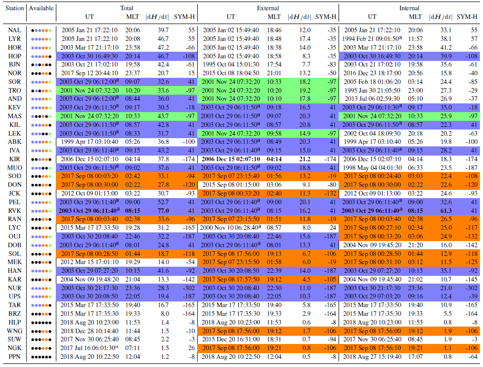
^a SC according to http://isgi.unistra.fr/, last access: 22 December 2022.

The maximum external $|\mathrm{d}\mathit{H}/\mathrm{d}t|$ values can be attributed to a handful of events. The Halloween storm in October 2003 is clearly the main source of the most intense $|\mathrm{d}\mathit{H}/\mathrm{d}t|$ values at the IMAGE stations, with the September 2017 storm generally as the replacement for those stations that did not have data from the Halloween storm. In addition to the October 2003 and September 2017 geomagnetic storms that mainly affected the stations in the middle of the IMAGE latitude range, the storm in November 2001 and an event in January 2005 caused the most intense values in northern Fennoscandia and Svalbard, respectively. The BJN station is located on an island between Fennoscandia and Svalbard, with some distance to Fennoscandia stations in the south and Svalbard stations in the north, and had its own most intense event. The southern IMAGE station TAR, which has provided data since 2001, observed the most intense values during the “St. Patrick's day” geomagnetic storm on 17 March 2015 (Wu et al., 2016). The stations south of TAR are fairly new to IMAGE and only have a few years of data. The maximum external $|\mathrm{d}\mathit{H}/\mathrm{d}t|$ at IMAGE, 21.2 nT s⁻¹, was observed at KIR during a geomagnetic storm in December 2006. Generally, the external $|\mathrm{d}\mathit{H}/\mathrm{d}t|$ effects of each event were limited in latitude and concentrated further south with decreasing SYM-H index values, as expected. Events associated with SCs, indicated in Table 1 by the superscript a, were naturally an exception, with positive values of concurrent SYM-H.

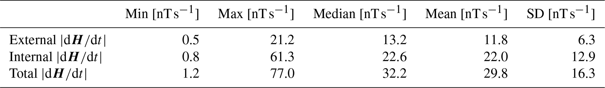
The most intense internal (61.3 nT s⁻¹) and also total $|\mathrm{d}\mathit{H}/\mathrm{d}t|$ (77.0 nT s⁻¹), observed by RVK, is attributed to the SC at the beginning of the Halloween storm. However, generally the events producing the most intense internal and, consequently, total $|\mathrm{d}\mathit{H}/\mathrm{d}t|$ values at IMAGE were more scattered in time than those that produced the maximum external values. Even during the same event, the maximum values at different stations did not typically occur at the same time. Most likely, this can be attributed to the complex ground conductivity structure as well as the temporal development of the external $\mathrm{d}\mathit{H}/\mathrm{d}t$ that drives induction. The intensity of the maximum external $|\mathrm{d}\mathit{H}/\mathrm{d}t|$ is fairly uniform across IMAGE (Table 2), with some dependence on data availability. The variability in the internal and, consequently, total maximum $|\mathrm{d}\mathit{H}/\mathrm{d}t|$, on the other hand, is much larger, due to the complexity of induction in the conducting ground.

Table 2 Minimum, maximum, median, mean, and standard deviation (SD) of the external, internal, and total $|\mathrm{d}\mathit{H}/\mathrm{d}t|$ from Table 1.

Next, we will study five events more closely that caused the most intense external $|\mathrm{d}\mathit{H}/\mathrm{d}t|$ values: 29 October 2003 at 06:11:50 UT (SC at the beginning of the Halloween storm), 30 October 2003 at 20:08:40 UT (substorm event of the Halloween storm), 24 November 2001 at 07:32:20 UT (storm-time pulsation event), 15 December 2006 at 02:07:10 UT (storm-time substorm event), and 17 April 1999 at 02:07:10 UT (storm-time substorm event). The last event is not represented in Table 1 but is responsible for very intense external $|\mathrm{d}\mathit{H}/\mathrm{d}t|$ values at several IMAGE stations.

3.1 Prenoon SC event on 29 October 2003 at 06:11:50 UT

On 29 October 2003 at 06:10:00 UT, a SC occurred, signifying the start of the Halloween storm. Figure 3e shows the SYM-H index around this time. The SC is marked by a vertical solid blue line. At 06:11:40–06:11:50 UT (vertical dashed black line in Fig. 3e), several IMAGE stations measured their most intense external $|\mathrm{d}\mathit{H}/\mathrm{d}t|$ between 1994 and 2018 (Table 1). At the same time, an intense (e.g., Hajra, 2022) GIC peak of 25 A (Fig. 3d) was recorded at MAN.

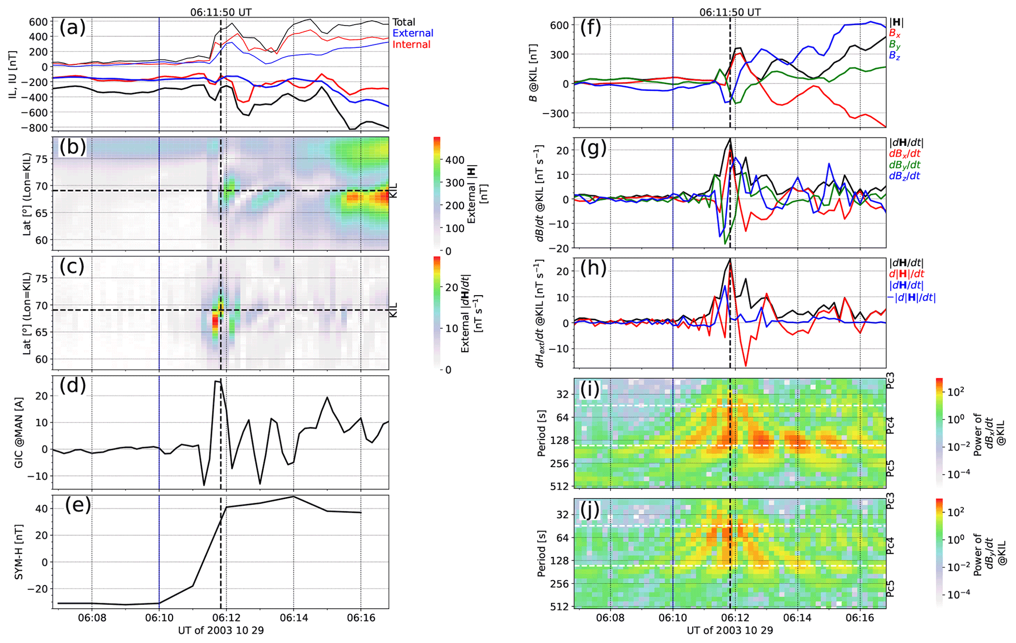
Figure 3 (a) Auroral electrojet indices derived from IMAGE data (Kauristie et al., 1996) ±5 min around the event on 29 October 2003 at 06:11:50 UT. The index derived from total (external + internal), external, and internal geographic ΔB_x from all available IMAGE stations is drawn with black, blue, and red colors, respectively. The thicker curves show the lower-envelope curve IL index and the thinner curves the upper-envelope curve IU index. (b) Latitude profiles of external ground $\left|\mathrm{\Delta }\mathit{H}\right|$ as a function of UT along the longitude of the KIL station (indicated in Fig. 4 by vertical black lines). (c) Latitude profiles of external 10 s $|\mathrm{d}\mathit{H}/\mathrm{d}t|$ as a function of UT along the longitude of the KIL station. (d) GICs in the natural gas pipe at MAN (location close to the IMAGE station NUR indicated in Fig. 4). (e) SYM-H index. (f) Geographic external ΔB_x, ΔB_y, and ΔB_z at the KIL station. (g) $\mathrm{d}{B}_x/\mathrm{d}t$, $\mathrm{d}{B}_y/\mathrm{d}t$, $\mathrm{d}{B}_z/\mathrm{d}t$ at KIL. (h) Time derivative of the external horizontal magnetic field vector ($|\mathrm{d}\mathit{H}/\mathrm{d}t|$), time derivative of the amplitude of the horizontal ground magnetic field vector ($\mathrm{d}\left|\mathit{H}\right|/\mathrm{d}t$), and the difference $|\mathrm{d}\mathit{H}/\mathrm{d}t|-\left|d\right|\mathit{H}|/\mathrm{d}t|$, which represents the contribution of the change in vector direction to $|\mathrm{d}\mathit{H}/\mathrm{d}t|$ at KIL. (i–j) Wavelet transform of $\mathrm{d}{B}_x/\mathrm{d}t$ and $\mathrm{d}{B}_y/\mathrm{d}t$ at KIL. The period ranges of the ultra-low-frequency (ULF) pulsation classes Pc3 (10–45 s), Pc4 (45–150 s), and Pc5 (150–600 s) (Jacobs et al., 1964) are shown with the horizontal dashed white lines. The vertical blue line indicates a SC at 06:10:00 UT, and the vertical dashed black line indicates the time of the extreme external $|\mathrm{d}\mathit{H}/\mathrm{d}t|$ observed at KIL.

Figure 3i–j show wavelet transforms (e.g., Torrence and Compo, 1998; Fligge et al., 1999) of external $\mathrm{d}{B}_x/\mathrm{d}t$ and $\mathrm{d}{B}_y/\mathrm{d}t$ at KIL. We use continuous wavelet transform with Morlet wavelets as given by the software available at https://pywavelets.readthedocs.io/en/latest/, last access: 22 December 2022 (Gregory et al., 2019). In addition to the time interval shown in Fig. 3f–g, we have included an equally long period of data before and after the interval of interest, i.e., analyzed an interval 3 times as long as that shown in Fig. 3f–g. The period ranges of the ultra-low-frequency (ULF) pulsation classes Pc3 (10–45 s), Pc4 (45–150 s) and Pc5 (150–600 s) (Jacobs et al., 1964) are indicated with horizontal dashed white lines. The wavelet transform reveals decaying oscillations around the 128 s period, as well as faster variations around 06:11:50 UT.

Figure 4a shows a map of the external equivalent current density (J, arrows) and the corresponding horizontal ground magnetic field magnitude ($\left|\mathrm{\Delta }\mathit{H}\right|$, color) on 29 October 2003 at 06:11:40 UT when the most intense external $|\mathrm{d}\mathit{H}/\mathrm{d}t|$ between 1994 and 2018 was measured at IVA, PEL, RVK, and DOB. The time derivatives of J and ΔH are displayed in Fig. 4b. Figure 4c–d show the same for 06:11:50 UT, when the most intense external $|\mathrm{d}\mathit{H}/\mathrm{d}t|$ was measured at KEV, MAS, KIL, ABK, and MUO. Figure 4b and d illustrate the geographical extent of the $|\mathrm{d}\mathit{H}/\mathrm{d}t|$ signature. Its temporal development explains the different times of maximum $|\mathrm{d}\mathit{H}/\mathrm{d}t|$ at different stations. The SOD station is displayed in these plots as one of the stations strongly affected by the signature, but in Table 1 it shows missing data for 29 October 2003. The reason is that time derivatives for the statistics were processed 1 d at a time, and any station with data gaps during that day was omitted because changes in station configuration produce artificial temporal changes in the resulting data at nearby stations. The time development of the ionospheric equivalent currents and the magnetic field they produce on the ground is further illustrated by the animation in the Supplement, IMAGE_20031029T060650_10sec_20031029T061650.mp4, which consists of frames similar to Figs. 3a–e and 4a and b on 29 October 2003 between 06:06:50 and 06:16:50 UT (10 min) with a 10 s time step.

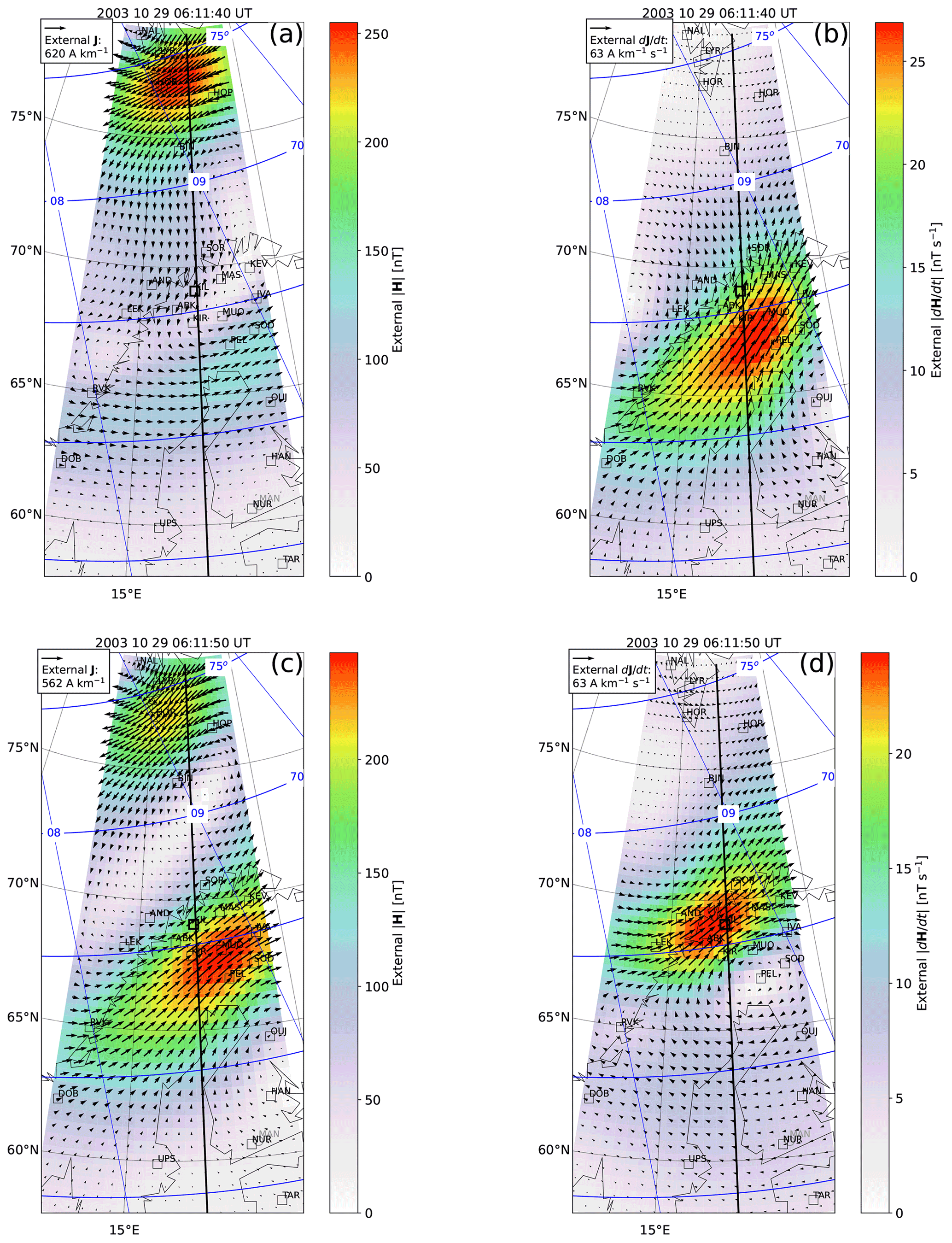
Figure 4 (a) External equivalent current density (J, arrows) and external horizontal magnetic field on the ground ($\left|\mathrm{\Delta }\mathit{H}\right|$, color) on 29 October 2003 at 06:11:40 UT when the largest external $|\mathrm{d}\mathit{H}/\mathrm{d}t|$ between 1994 and 2018 was measured at stations IVA, PEL, RVK, and DOB. (b) 10 s time derivative of external J ($\mathrm{d}\mathit{J}/\mathrm{d}t$, arrows) and of external ΔH ($|\mathrm{d}\mathit{H}/\mathrm{d}t|$, color). (c–d) The same as (a)–(b) but at 06:10:50 UT, when the largest external $|\mathrm{d}\mathit{H}/\mathrm{d}t|$ was measured at stations KEV, MAS, KIL, ABK, and MUO. In each panel, a vertical black line passing through the KIL station indicates the locations from which latitudes profiles are extracted to create a time series representation of the parameters in Fig. 3.

The SC caused the appearance, intensification, and northward propagation of the eastward electrojet (EEJ), tilted slightly from geomagnetic eastward to northeastward. The limited spatial extent indicates that this current is indeed an enhancement of the ionospheric EEJ and not an equivalent current representation of the sudden enhancement of the magnetopause currents (Fiori et al., 2014). The temporal evolution of the EEJ enhancement is illustrated in Fig. 3b and c, which present latitude profiles of $\left|\mathrm{\Delta }\mathit{H}\right|$ and $|\mathrm{d}\mathit{H}/\mathrm{d}t|$ as a function of UT along the longitude of the KIL station, indicated in Fig. 4 by vertical black lines. The auroral electrojet indices IL (thick curves) and IU (thin curves) (Kauristie et al., 1996) derived from total (external + internal), external, and internal IMAGE data in Fig. 3a only show a modest increase in the external IU during the SC.

Time series of the geographic external magnetic field components and their time derivatives at KIL are displayed in Fig. 3f–g. In agreement with Figs. 4 and 3a–c, they show a short-lived intensification of northeastward current passing over the station. The most intense external $|\mathrm{d}\mathit{H}/\mathrm{d}t|$ at 06:11:50 UT is associated with the appearance of the EEJ. Figure 3h shows the change of the external horizontal magnetic field vector ($|\mathrm{d}\mathit{H}/\mathrm{d}t|$, black), its amplitude ($\mathrm{d}\left|\mathit{H}\right|/\mathrm{d}t$, red), and their difference ($|\mathrm{d}\mathit{H}/\mathrm{d}t|-\left|\mathrm{d}\right|\mathit{H}|/\mathrm{d}t|$, blue), representing the contribution of the change in vector direction to $|\mathrm{d}\mathit{H}/\mathrm{d}t|$. $\mathrm{d}\left|\mathit{H}\right|/\mathrm{d}t$ is zero if the intensity of ΔH remains constant, but its direction can still change. According to Fig. 3h, the maximum external $|\mathrm{d}\mathit{H}/\mathrm{d}t|$ (black curve) is caused by the intensification of the EEJ (red curve), with practically no contribution from the change of direction in the current (blue curve).

The most intense external $|\mathrm{d}\mathit{H}/\mathrm{d}t|$ event observed at LYC (Table 1) on 10 November 2000 at 06:28:40 UT (∼ 09:00 MLT) was also associated with a SC. Examination of the event (not shown) reveals that it shared many similar features with the SC on 29 October 2003. In both cases the most intense $|\mathrm{d}\mathit{H}/\mathrm{d}t|$ was caused by an abrupt intensification and poleward propagation of the EEJ. Finally, we note that the appearance of a SC in the list of the largest $|\mathrm{d}\mathit{H}/\mathrm{d}t|$ events is a little fortuitous. The SC on 29 October 2003 just happened to occur at a time when the IMAGE network was in an optimal local time sector to measure very large variations.

3.2 Premidnight substorm event on 30 October 2003 at 20:08:40 UT

Figure 5 shows a substorm event that took place in the middle of the Halloween storm, on the evening of 30 October 2003. The format is similar to the corresponding panels in Figs. 3 and 4c–d, but it shows a time interval of 35 min instead of 10 min. MAN (Fig. 5d) shows an intense GIC peak of −49 A at 20:08:20–20:08:30 UT (the sign of the GIC indicates the direction of the current in the pipe, positive eastward). According to Fig. 5, an intensification and poleward and equatorward expansion of a WEJ occurred around 19:47:00 UT, typical for a local substorm onset. At 20:08:40 UT, the latitudinally wide, strong WEJ abruptly weakened (Fig. 5b), causing an intense time derivative signature over a long latitude range (Fig. 5c). The most intense external $|\mathrm{d}\mathit{H}/\mathrm{d}t|$ was observed at this time at the IMAGE stations OUJ, HAN, NUR, and UPS (Table 1). These stations are located in the southern part of IMAGE (Fig. 5k–l) and were not as much affected by the (10 s) SC signature on 29 October 2003 as the stations in the northern part of Fennoscandia (Fig. 4). The magnetic field time series at station OUJ (Fig. 5f–h) confirm the sudden weakening of the WEJ at 20:08:40 UT but also reveal wave activity (Fig. 5g) associated with the weakening. The wavelet transforms of external $\mathrm{d}{B}_x/\mathrm{d}t$ and $\mathrm{d}{B}_y/\mathrm{d}t$ (Fig. 5i–j) show wave activity across a wide range of periods but particularly around 128 s period. The time development is also illustrated by the animation in the Supplement, IMAGE_20031030T194340_10sec_20031030T201840.mp4, which is composed of frames similar to Fig. 5a–e, k, and l on 15 December 2006 between 01:52:10 and 02:22:10 UT (30 min) with a 10 s time step.

Figure 5 Data in a format similar to combined Figs. 3 and 4c–d from −25 to +10 min around the event on 30 October 2003 at 20:08:40 UT.

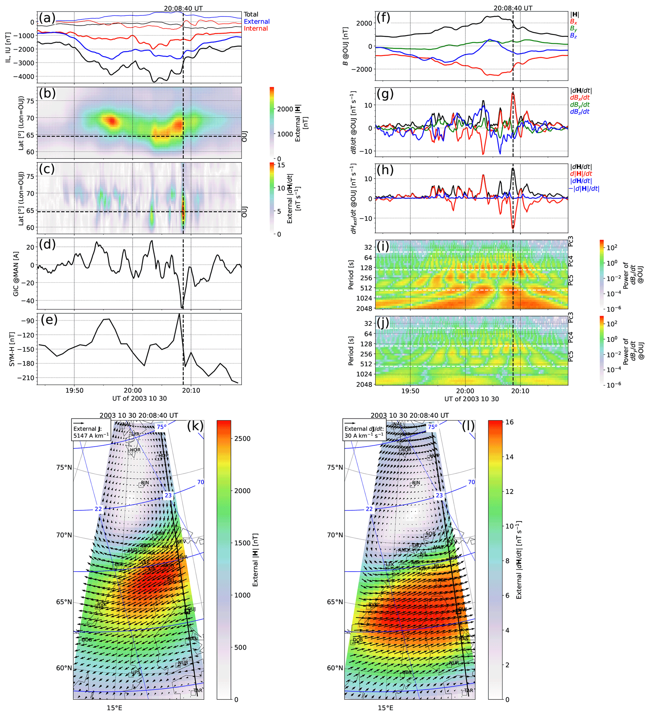
Comparison of Fig. 5b and e reveals that the two intensifications of the WEJ (∼ 19:53:00–19:58:00 and ∼ 20:02:00–20:08:40 UT) coincided with enhancements of the SYM-H index of a few tens of nanoteslas (nT). In the absence of direct solar wind drivers, increases of 20–40 nT in SYM-H after substorm onsets have been suggested to be caused by dipolarization, where the inner magnetosphere on the nightside is highly compressed, resulting in an increase in the ground $\left|\mathrm{\Delta }\mathit{H}\right|$ and SYM-H (Huang et al., 2004). The southward expansion of the WEJ that coincides with the SYM-H peaks supports this interpretation. Furthermore, the abrupt weakening and northward retreat of the WEJ at 20:08:40 UT coincides with the return of the SYM-H index back to the level preceding the enhancement, indicating a sudden recovery from dipolarization, possibly due to cessation of fast flows from a reconnection site farther downtail. It should be noted that this substorm event was very strong and produced the most intense external horizontal ground magnetic field ($\left|\mathrm{\Delta }\mathit{H}\right|$) between 1994 and 2018 at several IMAGE stations (Table 3).

Table 3 The same as Table 1 except for $\left|\mathrm{\Delta }\mathit{H}\right|$ instead of $|\mathrm{d}\mathit{H}/\mathrm{d}t|$.

Pulkkinen et al. (2005) have previously studied GICs and their relation to problems in the Swedish high-voltage power transmission system during the Halloween storm. They identified two periods during which problems in the power transmission system were observed: 06:10–07:05 UT on 29 October 2003 and 19:35–20:30 UT on 30 October 2003. These periods include our events (SC event at 06:11:40–50 UT on 29 October 2003 and substorm event at 20:08:40 UT on 30 October 2003). Pulkkinen et al. (2005) attributed the problems in operating the Swedish system during the storm broadly to substorms, storm sudden commencement, and enhanced ionospheric convection, all of which created large and complex geoelectric fields capable of driving large GICs. Our results further specify that the largest external $|\mathrm{d}\mathit{H}/\mathrm{d}t|$ values were caused by an abrupt intensification of an EEJ due to the compression of the Earth's magnetosphere and an abrupt weakening of a substorm WEJ, possibly in association with an expansion of the inner magnetosphere and the transition region between dipolar and tail-like field lines, respectively.

3.3 Prenoon pulsation event on 24 November 2001 at 07:32:20 UT

On 24 November 2001, a geomagnetic storm driven by an interplanetary coronal mass ejection (ICME) and its sheath occurred (Tsurutani et al., 2015). According to Tsurutani et al. (2015), two extremely intense substorms with a peak SuperMAG auroral electrojet index of −3839 and −3312 nT took place at ∼ 07:00–07:50 UT and at ∼ 13:45–14:18 UT, respectively. Our event with intense external $|\mathrm{d}\mathit{H}/\mathrm{d}t|$ at IMAGE occurred during the first substorm, at 07:32:20 UT. At this time, IMAGE was on the dayside, around 10:00 MLT. The first substorm began during a period of strong southward IMF in the sheath, but by the time of our event, IMF had turned northward. This is illustrated in Fig. 6, which shows solar wind, SYM-H, and auroral electrojet index data. Timing of the effects of solar wind data on the ground always contains some uncertainty (e.g., uncertainty due to the propagation from the observation point to the Earth's bow shock and the delay from the bow shock to the ionosphere), but it appears that the event may have coincided with a drop in the solar wind dynamic pressure (Fig. 6d) after a very high peak.

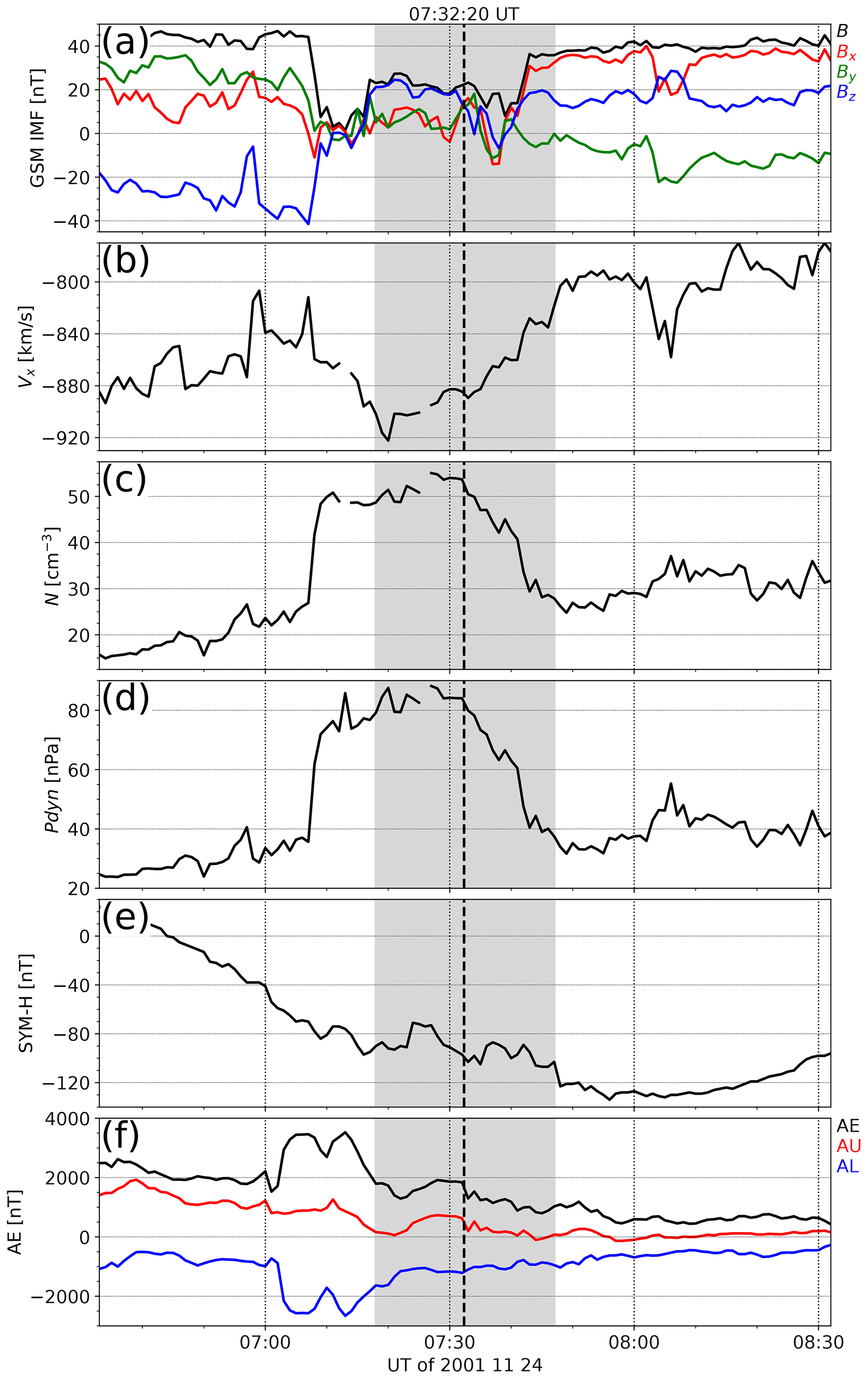
Figure 6 (a) Interplanetary magnetic field (IMF) magnitude and GSM (geocentric solar magnetospheric) components ±1 h around the event on 24 November 2001 at 07:32:20 UT. (b) GSM x component of the solar wind velocity. (c) Solar wind density. (d) Solar wind dynamic pressure. (e) SYM-H index. (f) Auroral electrojet indices. The time interval of Fig. 7 (30 min) is shaded in grey, and the time of the extreme $|\mathrm{d}\mathit{H}/\mathrm{d}t|$ event at IMAGE is indicated by the vertical dashed black line.

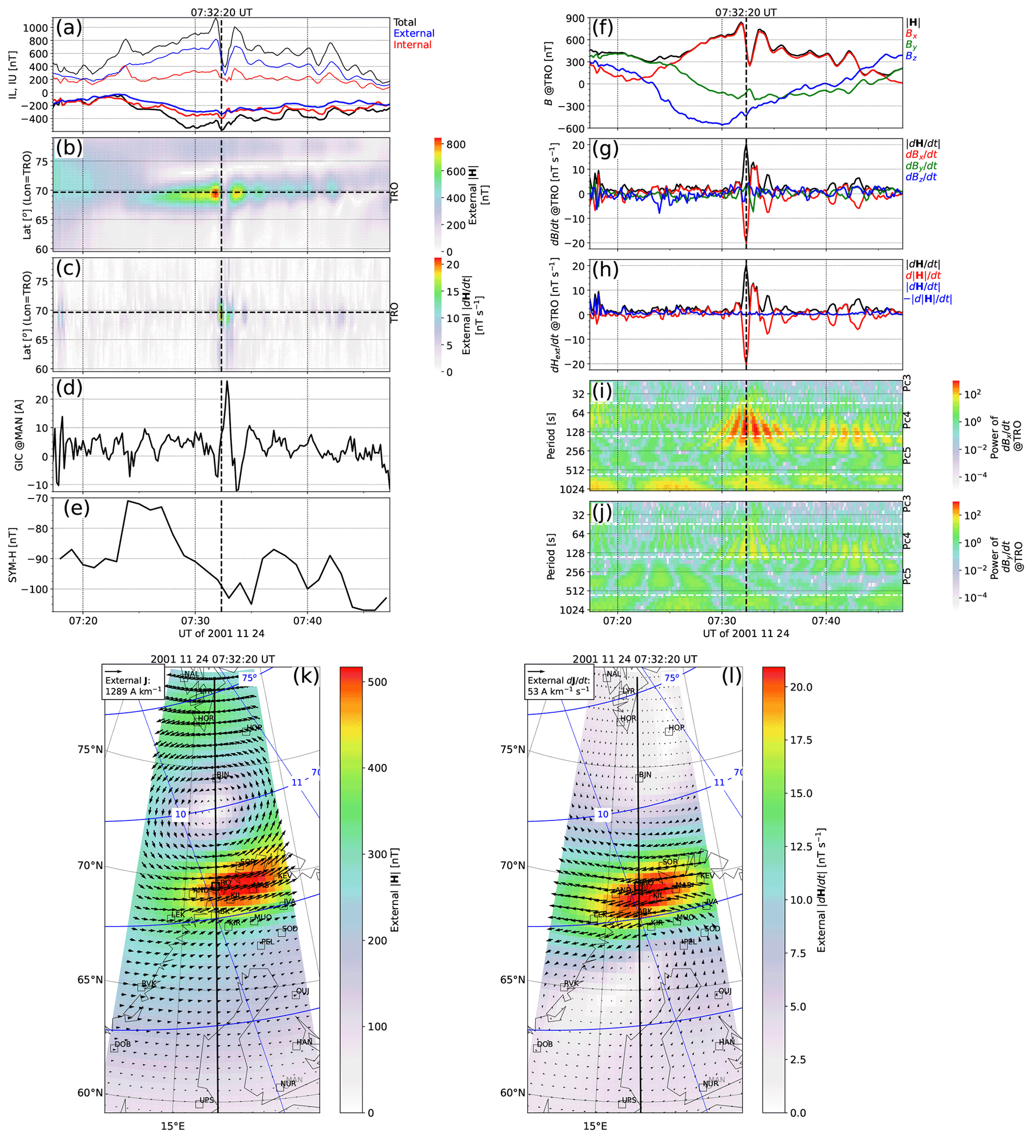
Figure 7 Data in a format similar to Fig. 5 ±15 min around the event on 24 November 2001 at 07:32:20 UT.

Figure 7 illustrates the event at IMAGE in a format similar to Fig. 5. At 07:32:20 UT, the most intense $|\mathrm{d}\mathit{H}/\mathrm{d}t|$ was observed at SOR, TRO, AND, and LEK (Table 1). According to Fig. 7l, the intense $|\mathrm{d}\mathit{H}/\mathrm{d}t|$ signature was concentrated in northern Fennoscandia. The KIL station is listed as not having data on 24 November 2001 due to some data gaps during the day but appears in Fig. 7k–l. Figure 7 shows that the intense $|\mathrm{d}\mathit{H}/\mathrm{d}t|$ was associated with the EEJ that was disrupted due to wave activity. A wavelet transform of $\mathrm{d}{B}_x/\mathrm{d}t$ and $\mathrm{d}{B}_y/\mathrm{d}t$ in Fig. 7i–j indicates wave activity around the 128 s period around and after 07:32:20 UT as well as faster variations in the Pc4 period range around 07:32:20 UT. The time development is also illustrated by the animation in the Supplement, IMAGE_20011124T071720_10sec_20011124T074720.mp4, which is composed of frames similar to Fig. 7a–e, k, and l on 24 November 2001 between 07:17:20 and 07:47:20 UT (30 min) with a 10 s time step.

Analogous to the SC event on 29 October 2003, it appears that the compression of the dayside magnetopause by intense dynamic pressure created an EEJ signature in the prenoon auroral ionosphere. Whereas intense $|\mathrm{d}\mathit{H}/\mathrm{d}t|$ on 29 October 2003 was associated with the abrupt appearance of the EEJ, in this event, intense $|\mathrm{d}\mathit{H}/\mathrm{d}t|$ is associated with the disappearance of the EEJ as the dynamic pressure weakened. The EEJ signature did not disappear abruptly but faded away during the time it took for the dynamic pressure to weaken. The disappearance of the EEJ, however, was not smooth but overlaid with decaying wave activity (Parkhomov et al., 1998). This pulsation activity caused the most intense $|\mathrm{d}\mathit{H}/\mathrm{d}t|$ by temporarily disrupting the EEJ. As can be seen in Fig. 7b–c, the pulsation signatures first appeared at lower latitudes and from there propagated northward, producing stronger variations where the ionospheric currents were stronger. The subauroral counterpart of these signatures appears to be responsible for the GIC peak of 26 A at 07:32:50 UT at MAN, close to the NUR magnetometer located at 60.5^∘ latitude.

Another pulsation event (not shown) with the most intense (although relatively weak) external $|\mathrm{d}\mathit{H}/\mathrm{d}t|$ in Table 1 was the event at southern IMAGE stations HLP and WNG on 20 August 2018 at 10:22:50–10:23:00 UT (∼ 12:00 MLT). The solar wind dynamic pressure during this event was nominal, but the solar wind speed was high, around 600 km s⁻¹.

3.4 Morning sector substorm event on 15 December 2006 at 02:07:10 UT

A SC occurred on 14 December 2006 at 14:14:18 UT and was followed later by a geomagnetic storm driven by fast solar wind and strong southward IMF (Fig. 8). The event of intense external $|\mathrm{d}\mathit{H}/\mathrm{d}t|$ at IMAGE took place at 02:07:10 UT, near the SYM-H minimum of the storm (Fig. 8e). Figure 9 shows the event at IMAGE in a format similar to Fig. 5. The most intense external $|\mathrm{d}\mathit{H}/\mathrm{d}t|$ observed by any IMAGE station between 1994 and 2018, 21.2 nT s⁻¹, was detected at the KIR station at 02:07:10 UT (∼ 04:00 MLT). Figure 9l shows that this was a relatively localized event peaking near KIR. Several nearby stations list this event as second largest after the Halloween storm. The event did not produce significant GIC peaks at MAN (Fig. 9d), most likely due to the relatively localized nature of the $|\mathrm{d}\mathit{H}/\mathrm{d}t|$ signature.

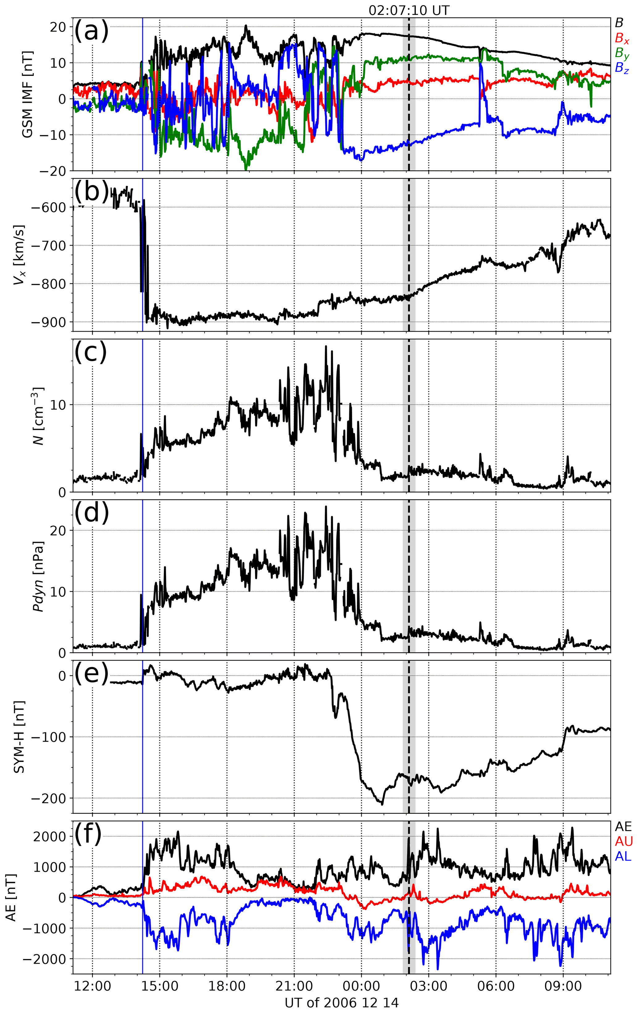
Figure 8 Data in a format similar to Fig. 6 from −15 to +9 h around the event on 15 December 2006 at 02:07:10 UT. The vertical blue line indicates a SC at 14:14:18 UT.

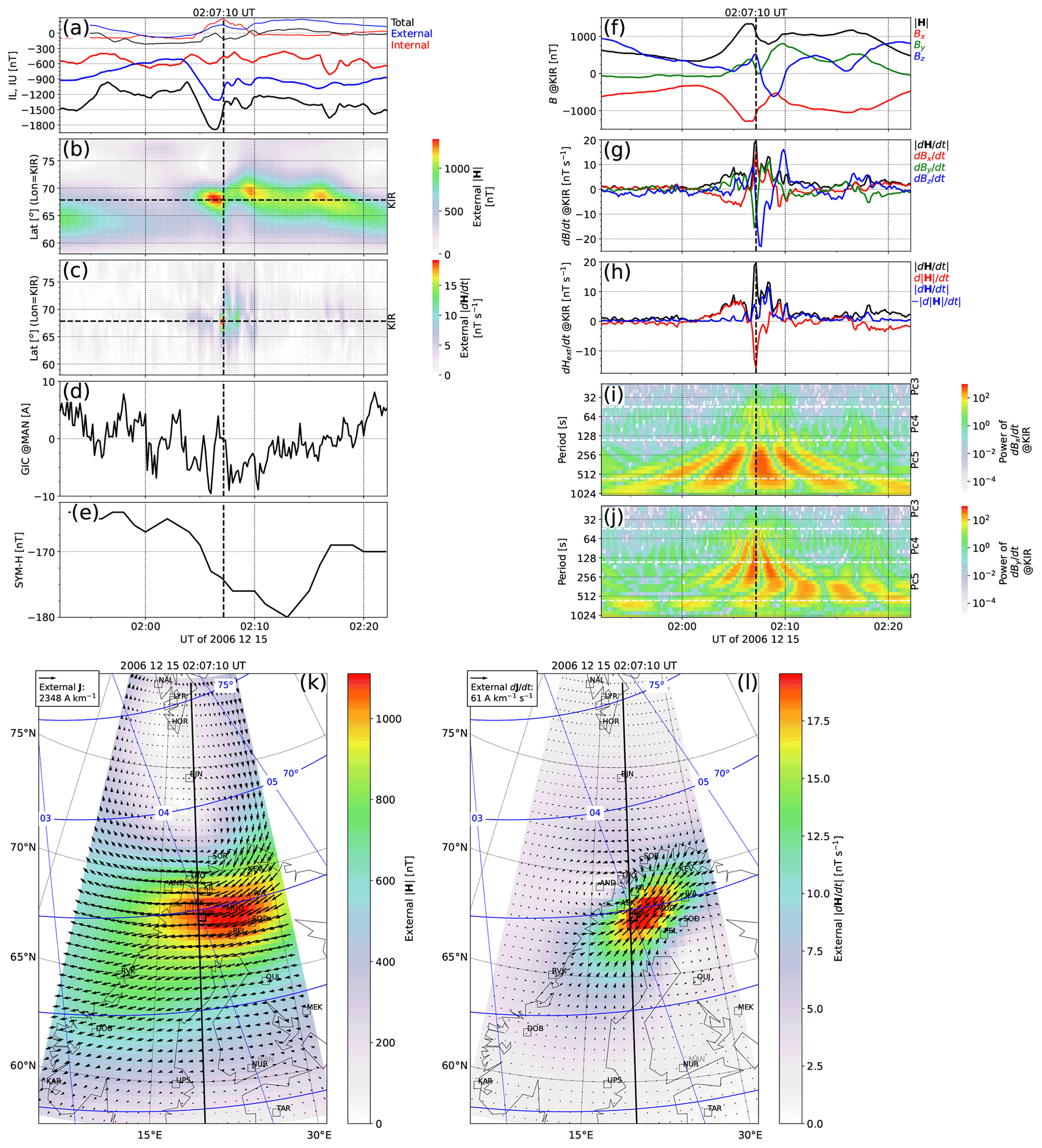
Figure 9 Data in a format similar to Fig. 5 ±15 min around the event on 15 December 2006 at 02:07:10 UT.

Figure 9b shows that the most intense $|\mathrm{d}\mathit{H}/\mathrm{d}t|$ occurred during a sequence of events during which the WEJ repeatedly intensified, jumped poleward, and slowly drifted equatorward. The most intense $|\mathrm{d}\mathit{H}/\mathrm{d}t|$ was associated with the sudden weakening (Fig. 9h) and poleward retreat of the WEJ at the end of the first of these cycles. The most intense $|\mathrm{d}\mathit{H}/\mathrm{d}t|$ during the Halloween substorm event (Sect. 3.2) also occurred when the WEJ suddenly weakened and retreated poleward. The large $\mathrm{d}{B}_y/\mathrm{d}t$ contribution to $|\mathrm{d}\mathit{H}/\mathrm{d}t|$ (Fig. 9g, l) in this event, while the ambient WEJ remained mainly east–west-oriented (Fig. 9f, k), indicates electrojet undulations, possibly associated with auroral streamer or omega band activity. Figure 10 shows the wavelet transform of external $\mathrm{d}{B}_x/\mathrm{d}t$ and $\mathrm{d}{B}_y/\mathrm{d}t$ at KIR for the longer time interval of Fig. 8 compared to that shown in Fig. 9i–j. The Ps6 period range 5–40 min (Jacobs et al., 1964) is indicated with the horizontal dashed white lines. According to Fig. 10, Ps6 activity occurred for several hours around 02:07:10 UT, during the time the SYM-H index slowly started to recover after the plummet of the main phase of the storm (Fig. 8). The time development is also illustrated by the animation in the Supplement, IMAGE_20061215T015210_10sec_20061215T022210.mp4, which is composed of frames similar to Fig. 9a–e, k, and l on 15 December 2006 between 01:52:10 and 02:22:10 UT (30 min) with a 10 s time step.

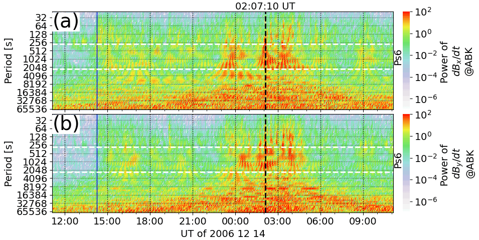
Figure 10 Wavelet transform of external $\mathrm{d}{B}_x/\mathrm{d}t$ and $\mathrm{d}{B}_y/\mathrm{d}t$ at KIR for the longer time interval from −15 to +9 h of Fig. 9 compared to the ±15 min shown in Fig. 9i–j for the event on 15 December 2006 at 02:07:10 UT. The period range of the ultra-low-frequency (ULF) pulsation class Ps6 (5–40 min) (Jacobs et al., 1964) are shown with the horizontal dashed white lines. The vertical solid blue line indicates the SC at 14:14:18 UT, and the vertical dashed black line indicates the time of the extreme external $|\mathrm{d}\mathit{H}/\mathrm{d}t|$ observed at KIR.

3.5 Morning sector substorm event on 17 April 1999 at 03:10:50 UT

Solar wind, SYM-H, and auroral electrojet data for our final event on 17 April 1999 are displayed in Fig. 11. Similar to the others, this event took place during a geomagnetic storm that started with a SC on 16 April 1999 at 11:24:54 UT and was followed by a clear sheath and ICME. The solar wind speed for this event was not high, but there was a strong sustained southward IMF associated with the front part of the ICME which drove the geomagnetic storm with a minimum SYM-H of around −100 nT. The event at IMAGE is illustrated in Fig. 12. It took place at 03:10:50 UT (05:00–06:00 MLT), close to the time of the SYM-H minimum of the geomagnetic storm. According to Fig. 12, the intense external $|\mathrm{d}\mathit{H}/\mathrm{d}t|$ was associated with a change of current direction from southwestward to westward in an intensified westward electrojet. Similar to the previous event, there is a large $\mathrm{d}{B}_y/\mathrm{d}t$ contribution to $|\mathrm{d}\mathit{H}/\mathrm{d}t|$, up-and-down motion of the WEJ, and Ps6 activity (Fig. 13), which indicate WEJ undulation. The time development is also illustrated by the animation in the Supplement, IMAGE_19990417T025550_10sec_19990417T032550.mp4, which is composed of frames similar to Fig. 12a–e, k, and l on 17 April 1999 from 02:55:50 to 03:25:50 UT (30 min) with a 10 s time step.

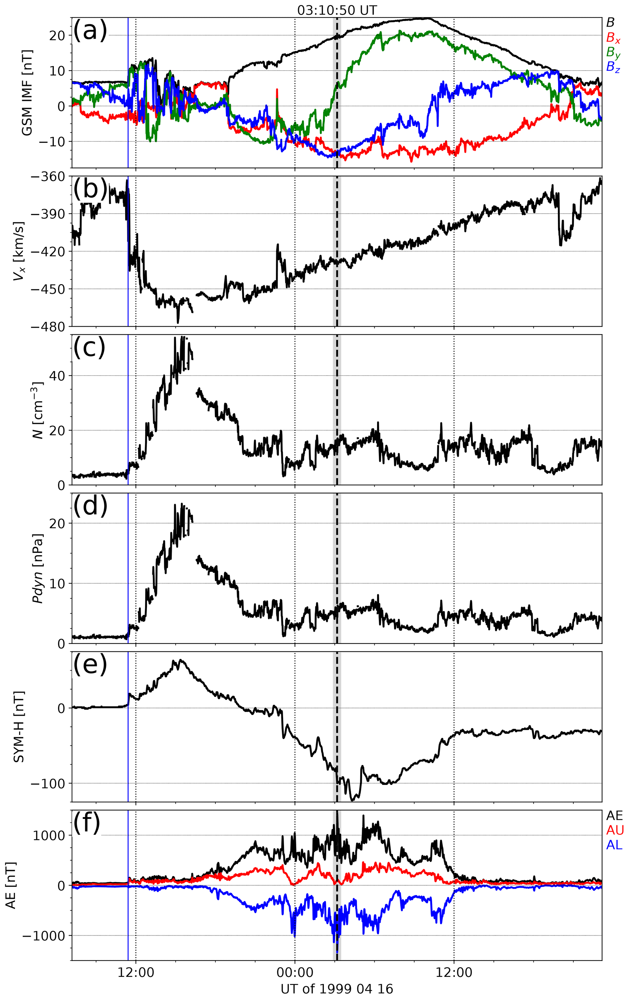
Figure 11 Data in a format similar to Fig. 6 ±20 h around the event on 17 April 1999 at 03:10:50 UT. The vertical blue line indicates a SC at 11:24:54 UT.

Other events of the most intense external $|\mathrm{d}\mathit{H}/\mathrm{d}t|$ in Table 1 associated with an intensified, undulating WEJ were the events at DON on 8 September 2015 at 01:15:00 (∼ 03:00 MLT), at SOD and RAN on 7 September 2017 at 23:15:40 UT (∼ 02:00 MLT), and at JCK on 8 September 2017 at 00:33:20 UT (∼ 03:00 MLT).

Figure 12 Data in a format similar to Fig. 5 ±15 min around the event on 17 April 1999 at 03:10:50 UT.

4 Discussion

We have examined five events in detail that were responsible for the most intense external $|\mathrm{d}\mathit{H}/\mathrm{d}t|$ in the IMAGE region between 1994 and 2018. All except the 17 April 1999 event are listed by Schillings et al. (2022) among the 27 strongest storms in 1980–2020 in terms of the number of observed intense “$\mathrm{d}B/\mathrm{d}t$” spikes worldwide. Our events and our interpretations are summarized in Table 4.

Table 4 Summary of the five studied events of the most intense external 10 s $|\mathrm{d}\mathit{H}/\mathrm{d}t|$ as observed by IMAGE between 1994 and 2018.

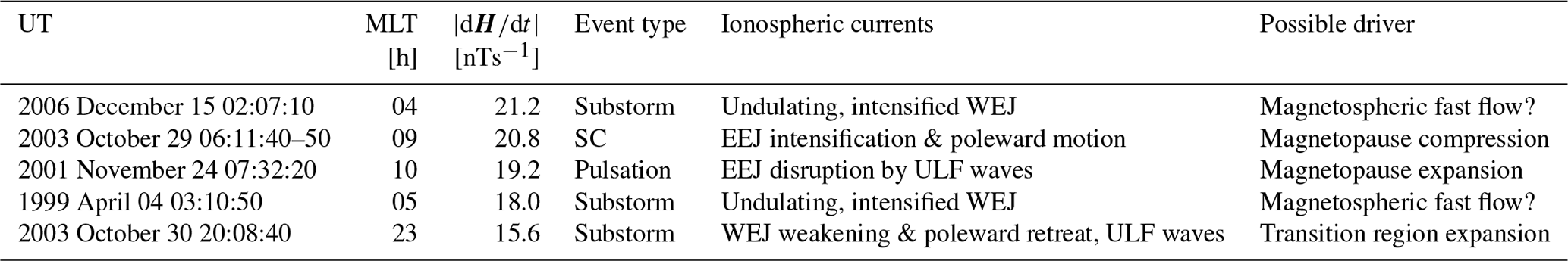
The five events represent all event types generally associated with intense $|\mathrm{d}\mathit{H}/\mathrm{d}t|$ or GIC: SCs, pulsations, and substorms. All were associated with geomagnetic storms preceded by SCs. Despite the wide range of event types and occurrence MLTs, the events share some common features: three out of the five events appeared to be directly associated with changes in the magnetospheric magnetic field configuration either due to compression (SC) or expansion (weakening of solar wind dynamic pressure or nightside dipolarization). In the other two events, the equatorward and poleward motion of the WEJ indicates some changes in the magnetospheric magnetic field configuration as well, although the cause is not clear. Fast magnetospheric flows associated with auroral streamer or omega band activity could be possible drivers.

What is noteworthy in our five events is that there are no substorm onsets or sudden intensifications of the WEJ among them. Viljanen et al. (2006b) have shown that substorm onsets are among the most significant drivers of intense $|\mathrm{d}\mathit{H}/\mathrm{d}t|$. Examination of the rest of the most intense external $|\mathrm{d}\mathit{H}/\mathrm{d}t|$ in Table 1 reveals that the most intense events at the northern IMAGE stations NOR on 8 October 2015 at 18:04:50 UT (∼ 21:00 MLT) and BJN on 4 October 1995 at 15:01:30 UT (∼ 18:00 MLT) were such intensifications. Furthermore, the events at the southern stations TAR and BRZ on 17 March 2015 at 17:33:50–17:35:30 UT (∼ 20:00 MLT) and at SOL, KAR, WNG, and NGK on 8 September 2017 at 17:57:50–17:56:00 UT (∼ 19:00 MLT) appear to be associated with the southward expansion of substorm currents. There can be several reasons why the more intense events do not include substorm onsets: one reason could be that induced currents play a very significant role in substorm onsets (e.g., Tanskanen et al., 2001), which would make them prominent in the examination of the total $|\mathrm{d}\mathit{H}/\mathrm{d}t|$ but not when only the external component is analyzed. Another reason could be that although substorm onsets generally produce large $|\mathrm{d}\mathit{H}/\mathrm{d}t|$, the most intense values require more extreme conditions: pre-existing intense ionospheric currents (the SC event was an exception) that are abruptly modified by rapid changes in the magnetospheric magnetic field configuration. Wave activity around the event can significantly enhance the $|\mathrm{d}\mathit{H}/\mathrm{d}t|$ signature. A third possibility is that, despite the long, continuous time series (1994–2018) of analyzed $|\mathrm{d}\mathit{H}/\mathrm{d}t|$, IMAGE has simply happened to be in the wrong MLT sector during the limited number of geomagnetic storms that have produced the most intense $|\mathrm{d}\mathit{H}/\mathrm{d}t|$ peaks worldwide. The mechanisms that produce the $|\mathrm{d}\mathit{H}/\mathrm{d}t|$ peaks during these storms would vary according to MLT, but globally the most intense peaks would be associated with substorm onsets in the appropriate MLT sector where IMAGE just did not happen to be located at the crucial moments.

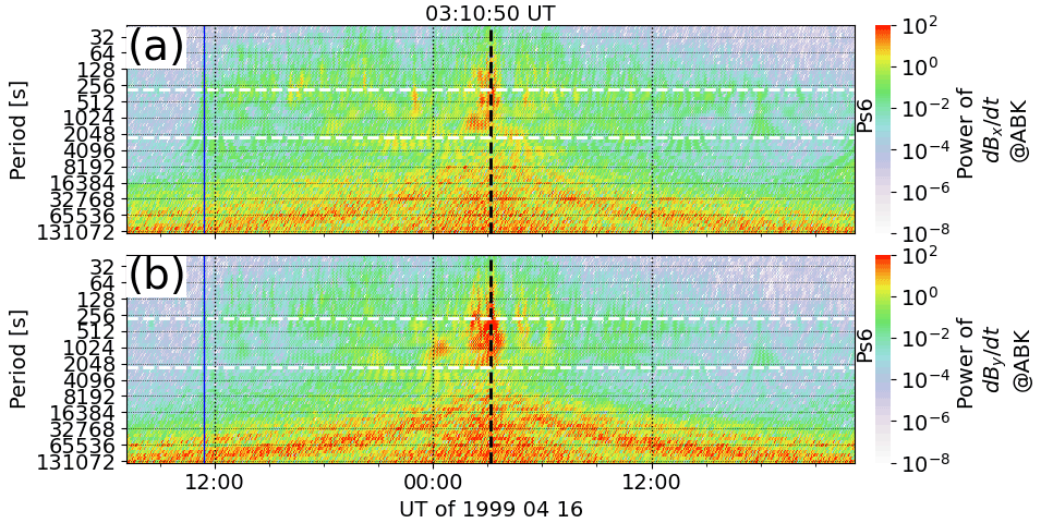
Figure 13 Data in a format similar to Fig. 10 ±20 h around the event on 17 April 1999 at 03:10:50 UT.

The second alternative agrees with the results of Viljanen et al. (2006b) and Engebretson et al. (2021). Viljanen et al. (2006b) examined the occurrence of maximum $|\mathrm{d}\mathit{H}/\mathrm{d}t|$ after substorm onsets at IMAGE stations during 1997 and 1999. They showed that the largest value of $|\mathrm{d}\mathit{H}/\mathrm{d}t|$ during substorms occurs most probably at about 5 min after the onset at stations with CGM (corrected geomagnetic coordinate) latitude less than 72^∘. At this time, the amplitude of the westward electrojet increases rapidly. Engebretson et al. (2021) showed the occurrence of maximum “$\mathrm{d}B/\mathrm{d}t$” events vs. time delay after substorm onset for five stations in Arctic Canada during 2015 and 2017, with MLATs (magnetic latitudes) ranging from 75.2 to 64.7^∘. There was no significant peak near 5 min after onset at any of these stations, and it was suggested that maximum $\mathrm{d}B/\mathrm{d}t$ events are not typically associated with substorm onsets but times of the most intense westward electrojet. The key difference between these apparently contradictory results is that whereas Viljanen et al. (2006b) examined the occurrence of maximum $|\mathrm{d}\mathit{H}/\mathrm{d}t|$ after all identified substorm onsets (with average maximum $|\mathrm{d}\mathit{H}/\mathrm{d}t|$ typically less than 2.5 nT s⁻¹), Engebretson et al. (2021) only considered intense $\mathrm{d}B/\mathrm{d}t$ events with maximum $\mathrm{d}B/\mathrm{d}t>\mathrm{6}$ nT s⁻¹. Thus, although the intensifying westward electrojet after substorm onset may be a typical source of moderate $|\mathrm{d}\mathit{H}/\mathrm{d}t|$ values (Viljanen et al., 2006b), the more rare events with strong $\mathrm{d}B/\mathrm{d}t>\mathrm{6}$ nT s⁻¹ tend to occur during times of the most intense westward electrojet (Engebretson et al., 2021). Engebretson et al. (2021) also showed that postmidnight $\mathrm{d}B/\mathrm{d}t$ events that occurred greater than 30 min after substorm onsets at the lowest latitude station (KJPK, 64.7^∘ MLAT) occurred during periods of gradual weakenings of the westward electrojet. These could be similar to our events with the undulating westward electrojet.

4.1 On the time resolution of $|\mathrm{d}\mathit{H}/\mathrm{d}t|$

Time resolution of the magnetic field data used to calculate the time derivative (Eq. 6) affects the amplitude and timing of the resulting $|\mathrm{d}\mathit{H}/\mathrm{d}t|$ peaks. As an example, Fig. 14 shows the total $|\mathrm{d}\mathit{H}/\mathrm{d}t|$ derived from 1, 10 s, and 1 min data at NUR around the SC signature on 29 October 2003 (Sect. 3.1) between 06:09:00 and 06:15:00 UT. The amplitude and location of the peak $|\mathrm{d}\mathit{H}/\mathrm{d}t|$ are clearly affected by the time resolution: 1 s $|\mathrm{d}\mathit{H}/\mathrm{d}t|$ had a peak value of 179.4 nT s⁻¹ at 06:11:29 UT, 10 s data had a peak value of 17.7 nT s⁻¹ at 06:11:50 UT, and 1 min data had a peak of 1.8 nT s⁻¹ at 06:13:00 UT.

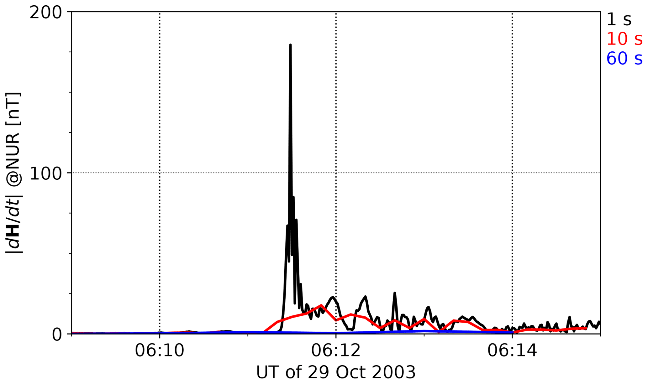
Figure 14 Time derivative of the total horizontal magnetic field ($|\mathrm{d}\mathit{H}/\mathrm{d}t|$) derived from 1, 10 s, and 1 min data at NUR on 29 October 2003 between 06:09:00 and 06:15:00 UT.

In addition to the SC, the Halloween storm on 29–31 October 2003 included intense substorm activity at nighttime and pulsations in the morning of 31 October 2003 (Panasyuk et al., 2004). Apart from the SC signature (Fig. 14), 10 s values are almost as large as 1 s values throughout the storm, whereas amplitudes derived from 1 min data are significantly weaker (data not shown). Thus, while proper description of the fast changes during SC events appears to require 1 s data, pulsations and substorms may be sufficiently described by 10 s $|\mathrm{d}\mathit{H}/\mathrm{d}t|$. The 1 min data, however, significantly underestimate the $|\mathrm{d}\mathit{H}/\mathrm{d}t|$ peaks.

4.2 Strong vs. extreme space weather events

Although the most intense events observed by IMAGE between 1994 and 2018 are certainly strong, they do not appear to be in any way exceptional compared to other strong events observed by IMAGE. This can be seen in Fig. 15, which shows a histogram of all total, internal, and external $|\mathrm{d}\mathit{H}/\mathrm{d}t|$ values at KIR between 1994 and 2018. The most intense external 10 s $|\mathrm{d}\mathit{H}/\mathrm{d}t|$ observed by IMAGE between 1994 and 2018, 21.2 nT s⁻¹, was measured at KIR in 15 December 2006 (Sect. 3.4). Functions in the form $a{\exp }^{-b|\mathrm{d}\mathit{H}/\mathrm{d}t|}$ (e.g., Myllys et al., 2014), where a and b are constants, have been fitted into the data points in Fig. 15 and can describe the occurrence of the most intense values quite well. Thus, our study may not provide information on truly extreme space weather conditions comparable to the Carrington geomagnetic storm (Clauer and Siscoe, 2006; Blake et al., 2021). Such storms are not covered by our observations and may be so much stronger than the observed events that data-based extrapolations cannot describe them. On the other hand, extreme value analysis by Wintoft et al. (2016) indicates that stations north of the magnetic latitude 60^∘ already include $|\mathrm{d}\mathit{H}/\mathrm{d}t|$ values that are close to the expected maxima, while more equatorward stations will measure larger values in the future.

Figure 15 Histogram of all total, internal, and external $|\mathrm{d}\mathit{H}/\mathrm{d}t|$ values observed by KIR between 1994 and 2018. The total number of data points is indicated in the parenthesis. The curves show $a{\exp }^{-b|\mathrm{d}\mathit{H}/\mathrm{d}t|}$ function fits to the data points, where a and b are constants.

4.3 Forecasting $|\mathrm{d}\mathit{H}/\mathrm{d}t|$ and GIC

As discussed by Pulkkinen et al. (2017), the horizontal geoelectric field expressed in time and space provides the key input to power grid operators to determine GIC and its impacts. A general risk analysis can be based on benchmark events, especially the most intense ones. Then it is possible to use long time series of geomagnetic recordings and provide the modeled geoelectric field for a large set of different events (e.g., Viljanen et al., 2014). For this purpose, it is also meaningful to use geomagnetic data from other locations as long as they are from approximately the same magnetic latitudes as the region of interest. Ideally, the external part of the variation field should be used, since it does not depend on effects due to local telluric currents (see Tables 1 and 3).

Concerning forecasting ground magnetic field variations from real-time L1 solar wind observations (e.g., Balan et al., 2017), our study helps in identifying events which are likely to cause large $|\mathrm{d}\mathit{H}/\mathrm{d}t|$ values (and large GIC): a strong SC or modification of pre-existing intense ionospheric currents by sudden changes in magnetospheric magnetic field configuration. This may be useful when tailoring empirical forecasts based on neural networks, for example. If the existence of intense “background” ionospheric currents can be predicted, or directly seen from real-time observations, then a general alarm of higher probability of a big $|\mathrm{d}\mathit{H}/\mathrm{d}t|$ event can be given. What obviously remains difficult is to anticipate whether there will be a trigger leading to intense $|\mathrm{d}\mathit{H}/\mathrm{d}t|$ and where and when this will take place. If the Halloween SC had begun a few minutes later, the largest $|\mathrm{d}\mathit{H}/\mathrm{d}t|$ values would obviously have occurred over the ocean. This shows that even if a SC can be quite definitely anticipated from L1 observations, there is still much uncertainty in predicting the most severely affected area precisely. Challenges also appear with substorms such as that of 30 October 2003 causing the Malmö blackout. Similar problems are faced by first-principle simulations, which are still far from optimal performance (e.g., Kwagala et al., 2020). Recently, Dimmock et al. (2021) have shown that by increasing the spatial resolution of global magnetohydrodynamic (MHD) models, the ability to model GIC can be improved. However, substorms still remain a problem because the simulations cannot capture the dynamics of the ionospheric currents that drive the complex external $\mathrm{d}\mathit{H}/\mathrm{d}t$. Our study shows that in addition to substorms, the most intense external $|\mathrm{d}\mathit{H}/\mathrm{d}t|$ can be caused by other event types as well. These event types are directly driven by solar wind disturbances, and current global MHD models work reasonably well in predicting the associated external geomagnetic disturbances. Whichever forecast methods are used, an experienced scientist-in-the-loop is needed for understanding uncertainties. Such experience can only be reached by analyzing a large set of events such as in this study.

5 Conclusions

We have compiled a list of the most intense external (due to ionospheric and magnetospheric electric currents), internal (due to induced telluric currents), and total (external + internal) $|\mathrm{d}\mathit{H}/\mathrm{d}t|$ (amplitude of the 10 s time derivative of the horizontal geomagnetic field) events at all IMAGE stations between 1994 and 2018 and examined five events in detail that caused the most intense external $|\mathrm{d}\mathit{H}/\mathrm{d}t|$ values. Our conclusions are as follows:

1. In agreement with previous results, the most intense external $|\mathrm{d}\mathit{H}/\mathrm{d}t|$ were broadly associated with sudden commencements (SCs), pulsations, and substorms during geomagnetic storms preceded by a SC and driven by intense southward IMF and often fast solar wind. Intense GIC peaks were associated with intense external $|\mathrm{d}\mathit{H}/\mathrm{d}t|$ nearby.

2. In the SC event, the most intense $|\mathrm{d}\mathit{H}/\mathrm{d}t|$ in the prenoon sector was caused by an intensification of the EEJ due to an abrupt compression of the magnetopause.

3. In the pulsation event, the most intense $|\mathrm{d}\mathit{H}/\mathrm{d}t|$ in the prenoon sector was caused by disruption of the EEJ due to wave activity during a magnetopause expansion as an intense solar wind dynamic pressure weakened. This event took place during the sheath of an ICME.

4. In the premidnight substorm event, the most intense $|\mathrm{d}\mathit{H}/\mathrm{d}t|$ was caused by sudden weakening and poleward retreat of the WEJ associated with wave activity. The WEJ weakening and poleward retreat coincided with an inferred weakening of dipolarization and, consequently, expansion of the transition region in the magnetosphere.

5. In the two morning sector events associated with substorm activity during ICME clouds, the most intense $|\mathrm{d}\mathit{H}/\mathrm{d}t|$ was caused by an intensified, undulating WEJ. In one case, weakening of the WEJ and, in the other, change in the current direction produced the most intense signature. The northward and southward motion of the entire WEJ indicates corresponding changes in the magnetospheric magnetic field configuration. Fast magnetospheric flows associated with auroral streamer or omega band activity could be possible drivers.

6. Despite being associated with various event types and occurring at different local time sectors, there were common features among the drivers of most intense $|\mathrm{d}\mathit{H}/\mathrm{d}t|$ values: pre-existing intense ionospheric currents (the SC event was an exception) that were abruptly modified by sudden changes in the magnetospheric magnetic field configuration.

7. While the most intense external $|\mathrm{d}\mathit{H}/\mathrm{d}t|$ events at adjacent stations typically occurred simultaneously, the most intense internal and total $|\mathrm{d}\mathit{H}/\mathrm{d}t|$ events were more scattered in time, most likely due to the complexity of induction in the conducting ground. From the analysis viewpoint, field separation is useful, since it removes the complicated contribution by induced currents, especially in $|\mathrm{d}\mathit{H}/\mathrm{d}t|$.