the Creative Commons Attribution 4.0 License.
the Creative Commons Attribution 4.0 License.
 | 01 Dec 2022
Signature of gravity wave propagations from the troposphere to ionosphere
Hisao Takahashi
Cosme A. O. B. Figueiredo
Patrick Essien
Cristiano M. Wrasse
Diego Barros
Prosper K. Nyassor
Igo Paulino
Fabio Egito
Geangelo M. Rosa
Antonio H. R. Sampaio
We observed a gravity wave (GW) signature in the OH emission layer in the upper mesosphere, and 4 h later, a medium-scale travelling ionospheric disturbance (MSTID) in the OI 630 nm emission layer. Spectral analysis of the two waves showed that both have almost the same wave characteristics: wavelength, period, phase speed and propagation direction, respectively, 200 km, 60 min, 50 m s−1, toward the southeast. From the gravity wave ray-tracing simulation for the mesospheric gravity wave, we found that the wave came from a tropospheric deep convection spot and propagated up to the 140 km altitude. Regarding the same wave characteristics between mesospheric GW and ionospheric MSTID, the two possible cases are investigated: a direct influence of the GW oscillation in the OI 630 nm emission height and the generation of a secondary wave during the GW breaking process. This is the first time to report an observational event of gravity wave propagation from the troposphere, mesosphere to thermosphere–ionosphere in the South American region.
- Article
(5484 KB) - Full-text XML
- BibTeX
- EndNote


A deep cloud convection in the troposphere generates vertical (up and down) air-mass movement launching a variety of gravity waves into the stratosphere. Atmospheric gravity waves (GWs) have important roles in transporting the energy and momentum from the lower to upper atmosphere and ionosphere. A part of energy and momentum is deposited in the mesosphere lower thermosphere (MLT) region through wave breaking and altering the background wind field. Some of the GWs produce secondary waves and propagate further upwards into the thermosphere where it modulates ionospheric plasma (Hocke and Schlegel, 1996; Nicolls et al., 2014). A part of medium-scale travelling ionospheric disturbances (MSTIDs) has its origin in the passage of gravity waves in the ionosphere (Otsuka, 2018). Observations of GW propagation in the thermosphere have been carried out by many researchers since Hines (1960) presented theoretical background for the GW propagation in the ionosphere. Rottger (1973) suggested the role of GWs in the ionospheric irregularities.
GW observations in the mesosphere have been carried out by measuring short period temporal variation of the mesospheric airglow (hydroxyl and atomic oxygen OI 557.7 nm emissions) by airglow photometers in 1970–1990 (e.g. Takahashi et al., 1999). After 1990, airglow digital imagers were used to monitor GWs in two-dimensional forms (e.g. Taylor et al., 2009; Dare-Idowu et al., 2020; Nyassor et al., 2021). Dynamical processes in the mesosphere to thermosphere were studied by OH and oxygen 630.0 nm airglow imaging by Kubota et al. (2000), Taori et al. (2013), and most recently by Ramkumar et al. (2021). In case of GWs in the stratosphere, satellite-onboard GPS radio occultation measurements have made it possible to observe GWs by vertical profile of the temperature variability on a global scale (Tsuda, 2014; Xu et al., 2017).
There are many previous works on the GW propagations in the stratosphere, mesosphere, and ionosphere individually. However, it has been difficult to monitor an event of GW propagating through the troposphere up to the ionosphere. Smith et al. (2013) observed GW waves in the OH and OI 557.7 nm emission layers in the mesosphere to lower thermosphere (MLT) region (85–100 km) and OI 630.0 nm emission layer (around 240 km altitude) in the thermosphere and discussed on the mountain waves from the mesosphere to ionosphere. They attributed the wave structure in the ionosphere as due to secondary waves. Azeem et al. (2015), for the first time, reported the occurrence of circular GW structures in the stratosphere, mesosphere, and ionosphere during a tropospheric convective storm. They observed concentric wave structures in the stratosphere by the Atmospheric Infrared Sounder (AIRS) onboard Aqua satellite (https://airs.jpl.nasa.gov/, last access: 30 September 2022), and by an optical imaging radiometer (VIIRS) onboard Suomi satellite (https://www.nasa.gov/mission_pages/NPP/main/index.html, last access: 30 September 2022), and in the ionosphere by ground-based GPS receivers. Prior to this work, Nishioka et al. (2013) has reported concentric gravity waves in the ionosphere which were induced by a severe convective system (supercell) in the troposphere. The concentric waves lasted for more than 7 h. Nyassor et al. (2021) reported the first mesospheric concentric gravity waves excited by thunderstorm. Takahashi et al. (2020) presented the generation and propagation of MLT GWs and concentric MSTIDs in the ionosphere during a deep convection activity in the troposphere over the South American continent.
Regarding propagation of GWs from the lower to upper atmosphere, Vadas (2007), for the first time, studied propagation property of GWs from the troposphere to the thermosphere for the horizontal wavelength of 10 to 1000 km and the period of 10 to 100 min. The author presented the GW dissipation altitudes depending on their horizontal wavelength and period. In case of the horizontal wavelength of 200 km and its period of 60 min, for example, the model predicts dissipation above 120 km altitude. It means that the dissipation produces a body force and generates secondary waves.
There is a difficulty to observe a gravity wave from its origin (source) in the troposphere following up to the thermosphere. During the upward propagation, it could change its wave characteristics under the background atmospheric condition, dissipating and producing secondary waves changing the horizontal wavelength, phase speed, and propagation direction (Vadas and Crowley, 2010). It would take several hours to reach from the troposphere to the mesosphere lower thermosphere (Vadas and Liu, 2013), which makes it difficult to follow the wave step by step. Recent observation of the concentric wavefronts in the stratosphere, mesosphere, and thermosphere by Azeem et al. (2015) would be rather a rare case. Further observational evidence would be necessary to clarify the propagation processes. The purpose of the present work is to report a case of gravity wave propagation directly from a tropospheric convection to the mesosphere and thermosphere/ionosphere. For investigating the propagation of gravity waves, data from the airglow OH imager in the mesosphere, OI 630 nm imager from the thermosphere/ionosphere, and ionosondes are used.
Airglow observation has been carried out at Bom Jesus da Lapa (hereafter BJL), 13.3∘ S, 43.5∘ W, geomag.14.1∘ S, since 2019. The observation site is located under the equatorial ionospheric anomaly (EIA) belt. Equatorial plasma bubbles can also be frequently observed. An all-sky airglow imager equipped with 3 in. optical interference filters (for 630.0, 557.7 and OH-NIR (710–930 nm)) takes 180∘ wide images with a time sequence of ∼ 5 min. Exposure time for each filter is 15 s for the OH-NIR and 90 s for the OI 630.0 and 557.7 nm images. The imager characteristics have been presented by Wrasse et al. (2021). In the present study we used the image data from December 2019 to September 2020. During this period, we selected 13 d of observation to analyse wave structures in the OI 630 nm images.
In the present work, the data from the ionosondes were used to observe the vertical drift of the F-layer and to calculate the electron density profile. Three digital ionosondes (DPS-4) (http://www.digisonde.com/instrument-description.html, last access: 30 September 2022) have been operated, one at São Luís (2.6∘ S, 44.2∘ W, geomag. 3.9∘ S), Fortaleza (3.9∘ S, 38.4∘ W, geomag. 6∘ S), and Cachoeira Paulista (22.7∘ S, 45.0∘ W, geomag. 18.1∘ S). The DPS-4 sounder has a 500 W peak power, covering a frequency range from 0.5 to 30 MHz. Ionograms are taken with a time interval of 10 min.
3.1 OH images
On the night of 18–19 January 2020, around 22:30 to 23:30 UT (19:30–20:30 LT), the airglow OH images showed two wave structures passed over BJL. Figure 1 shows the OH images at the moment of one of the wavefronts passing over the zenith. The images are projected on the geographic coordinates. The horizontal extension of the image is approximately 500 km and the blue dot indicates the location of the BJL observation site. In Fig. 1a, there are two wave structures, one is shorter wavelength in the northwest side of the image (top left side) (GW-1) and another is a longer wavelength, one wavefront over the zenith (blue dot) and the other at the southeast (SE) portion, indicated by the blue arrows (GW-2). Three sequential images with a time interval of 10 min indicate that the wavefront is moving toward SE (indicated by a red arrow in Fig. 1b). The propagation mode can be clearly seen if keograms are made by using the meridional and longitudinal cuts as a function of time. Figure 2 shows the keograms (zonal and meridional cuts) between 22:30 and 28:30 (04:30) UT. Looking at the GW-2, two bright bands propagating from north (N) to south (S) and west (W) to east (E) can be seen. The broad bright band passing over the zenith from northeast (NE) to southwest (SW) through the night is the galactic Milky Way.
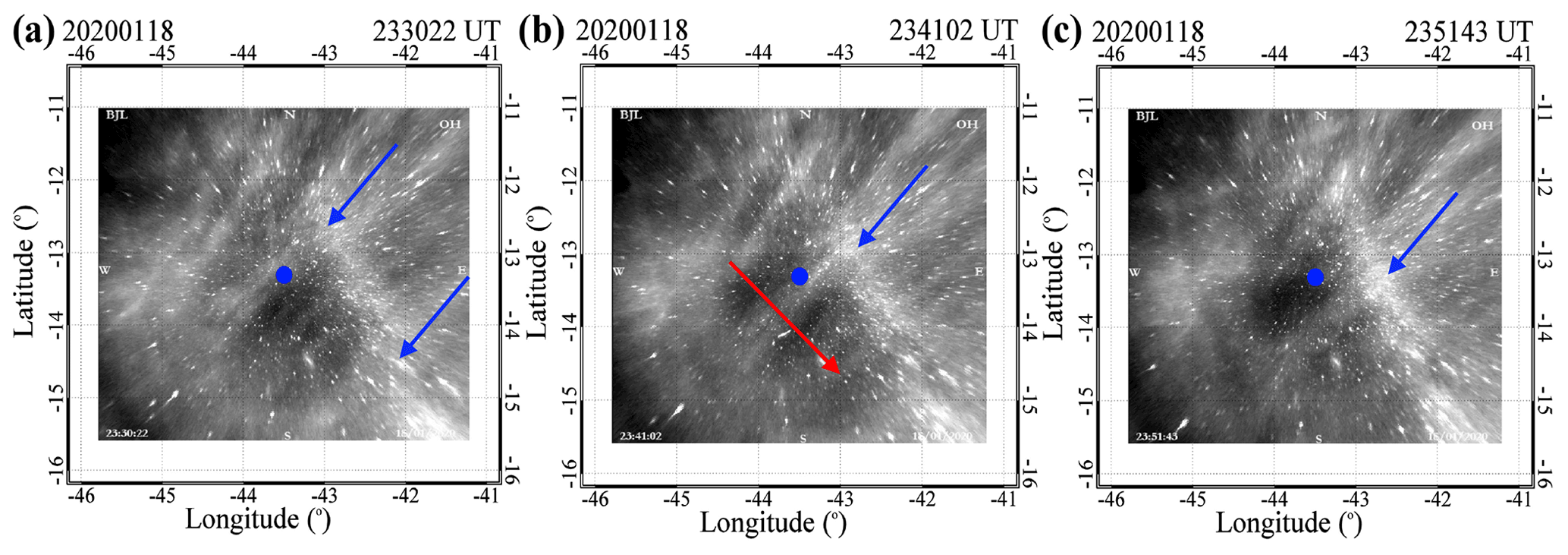
Figure 1Geographically coordinated OH images observed at Bom Jesus da Lapa (BJL), 13.3∘ S, 43.5∘ W, geomag. 14.1∘ S, on the night of 18–19 January 2020 at 23:30 UT (a), 23:41 UT (b), and 23:51 UT (c). Blue dots indicate the zenith of BJL. The blue arrows indicate the wave fronts of the longer wavelength one (GW-2). The red arrow indicates the direction of propagation.

Figure 2Keograms of OH images observed at BJL in the night of 18–19 January 2020. The zenith crossing sliced image along the W–E direction (a) and the S–N direction (b) are shown as a function of time from 22:00 to 30:00 (06:00) UT. The red colour rectangular boxes are where the FFT (fast Fourier transform) spectral analysis was taken.
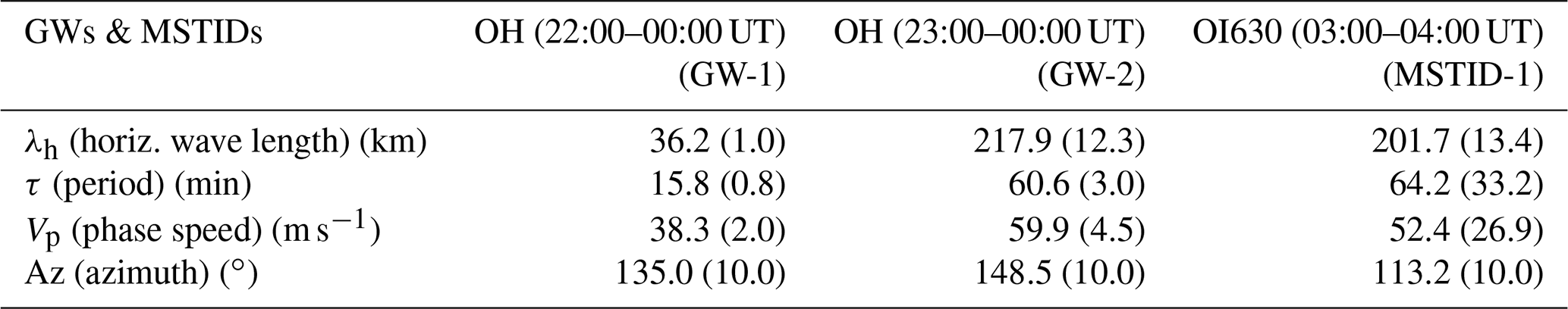
For calculating the wave characteristics (horizontal wavelength, period, phase velocity), we used fast Fourier transform (FFT) spectral analysis (Wrasse et al., 2007; Figueiredo et al., 2018; Essien et al., 2018). Image samples used in the calculation are indicated by red boxes in Fig. 2. The wave characteristics of the longer wave (GW-2) are the horizontal wavelength of 217.9 ± 12 km, the period of 60.6 ± 03 min, the phase speed of 59.9 ± 5 m s−1, and the propagation direction of 148.5 ± 10∘ (clockwise from north in degrees). For the short wave (GW-1), the wave characteristics were also obtained: the horizontal wavelength of 36.2 ± 1 km, the period of 15.8 ± 0.8 min, the phase speed of 38.3 ± 2 m s−1, and the propagation direction of 135.0 ± 10∘.
3.2 OI 630 nm image
Figure 3 presents three sequential images of the OI 630 nm emission between 03:20 and 03:48 UT. The top three panels are original images and the bottom three panels are the residual images which are subtracted from the 1 h averaged image. From the residual images, one can see two dark bands in the southwest of BJL propagating toward east, which seem to be the medium-scale travelling ionospheric disturbance, named as MSTID-1. We checked any contamination of the OH emission in the OI 630 nm image. No such wavelike structure could be seen in the OH images during the same period. The bright OI 630 emission intensity over the northwest part of the sky should be the midnight downward drift of the F-layer accompanied by the midnight temperature maximum (MTM) in the thermosphere (Colerico et al., 1996; Figueiredo et al., 2017). One can also notice the presence of the equatorial plasma bubbles (EPBs) (at least two depletions) in the northwest of BJL, which are also drifting toward the east. The difference between the EPBs and MSTID-1 is clear to see. The EPBs are extending from the Equator side and the MSTID is elongated from the south. During the 28 min of the time interval, from Fig. 3a to c, a dark band moved toward the east by ∼ 90 km. In order to get the wave characteristics of MSTID-1 from the OI 630 images, we used the FFT spectral analysis for the OI 630 keogram (not shown here), which is similar to the OH image analysis mentioned above (Wrasse et al., 2007). The results are the horizontal wavelength of 201.7 ± 13 km, the period of 64.2 ± 33 min, the phase speed of 52.4 ± 27 m s−1, and the propagation direction of 113.2 ± 10∘. The characteristics of the wave propagation in the OH emission layer and OI 630 nm emission layer are summarized in Table 1. The movement of wave fronts of MSTID-1 is presented in the supporting file (OI 6300_movie.mp4).

Figure 3Geographically coordinated OI 630 nm images observed at Bom Jesus da Lapa (BJL) at 03:20 (a, d), 03:34 (b, e), and 03:48 UT (c, f) on the night of 18–19 January 2020. The top three images are original and the bottom three images are residual subtracted from the 1 h averaged image. Blue dots indicate the location of BJL. MSTID-1, EPBs (upper left corner), and MTM can be seen (see text).
Table 1Wave Characteristics obtained by the OH images in the MLT region (GW-1 and GW-2), and OI 630 nm images in the thermosphere (MSTID-1). The values in parentheses are error ranges. “Az” indicates the propagation direction (clockwise from north).
Through the evening to midnight over the Bom Jesus da Lapa (BJL) airglow observation site (17∘ S, 38∘ W) on 18–19 January 2020, we observed a relatively long wavelength and slow speed GW (GW-2) in the OH emission layer (∼ 87 km altitude) at around 23:00 UT. In 4 h later (03:00 UT), we observed a wave structure in the OI 630 nm emission layer (∼ 240 km altitude) (MSTID-1). The two different waves, one from MLT and the other from the thermosphere, had almost the same wave characteristics, i.e. a same horizontal wavelength (210 ± 10 km), same period (62 ± 5 min), and the same phase speed (55 ± 5 m s−1). The propagation directions of the two emissions, however, are slightly different, OH showing 149∘ N against OI 630 being 113∘ N, the difference of 36∘. The OH wavefronts are extended longer than 500 km. On the other hand, the OI 630 wave was limited in the southern sky with a relatively short duration (∼ 60 min). Such coincident occurrence of the wave structure called our attention to further investigate whether these waves have the same origin from the lower atmosphere, i.e. both are primary waves, or one of the waves in the thermosphere was due to a secondary wave generated in the lower atmosphere.
4.1 GW ray tracing and tropospheric convection origin
For studying the wave propagation, we used a wave ray-tracing method (Paulino et al., 2013; Vadas et al., 2019; Nyassor et al., 2021) to find out the source of the waves in the lower atmosphere. The wind model used in this work was according to the NRLMSISE-00 (Picone et al., 2002) and horizontal wind model (HWM14) (Drob et al., 2015). Figure 4 presents the ray-tracing trajectories of the GW-2 for the case of no-wind and with-wind model.
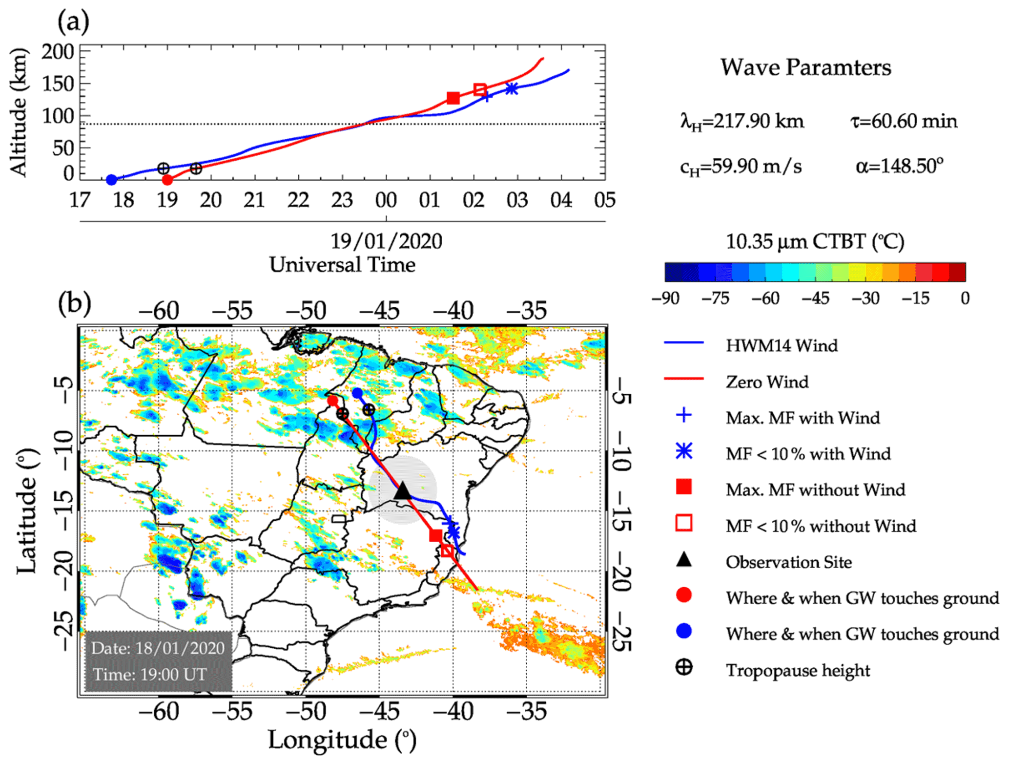
Figure 4Ray tracing (backward and forward) of the observed gravity wave (λh=217.9 km) starting at 87 km altitude at BJL on the night of 18 January 2020 at 23:30 UT. The vertical trajectory versus time (a) and horizontal distance (b) are shown. The red line is of the case of no-wind and the blue line is of the with-wind model. The blue triangle is the starting point of the ray tracing. The background map is the cloud top temperature from NOAA GOES-16 meteorological satellite data (10.35 μ) on 18 January 2020 at 19:00 UT.
The simulation started from 87 km altitude at 23:30 UT and went down (backward tracing) to the ground level at around 19:00 UT, crossing the tropopause (∼ 15 km) at around (7.0∘ S, 46.5∘ W) at 19:30 UT. There is a difference of around 200 km of the tropopause crossing positions between the no-wind and with-wind trajectories, which can be assumed to be an error range in the present study. Then, we search for any convective system in this region. Figure 4 also shows the cloud top temperature map produced by GOES-16 (10.35 μ radiation map) at 19:00 UT (https://www.cptec.inpe.br/, last access: 30 September 2022). The convection system spread over the tropical zone 0–10 S can be seen. It is the Intertropical Convergence Zone (ITCZ). One can notice that there is the lowest temperature spot (−80 ∘C) at (8.5∘ S, 46.5∘ W), where a deep convection was in progress. One can notice that this convection spot is located very close (in an error range of 200 km) to the GW-2 trajectory at the tropopause height. According to the GOES-16 maps, this convection spot started at around 18:00 UT, developing into a much larger area from 19:00 to 23:00 UT and decreasing the intensity after 00:00 UT. During the 5 h of activity, the convection spot should generate up and down streams inside of the convection cell producing a variety of GWs. The present ray tracing suggests that the observed gravity wave in the OH emission layer started from this convection spot propagating up to the lower thermosphere.
4.2 GW breaking in the thermosphere and generation of a secondary wave
The forward ray tracing shown in Fig. 4, on the other hand, went up to 130 km with the momentum flux in the maximum and then it lost the amplitude of oscillation at around 140 km, indicating dissipation of the wave energy. The wave dissipation occurred at the location of (18∘ S, 40∘ W) where we observed the wave structure in the OI 630 nm image starting at around 03:00 UT. According to Vadas and Crowly (2010), GW dissipation produces a body force and generates secondary waves. The secondary waves have a variety of wave characteristics. In our present case, we understand that the primary wave observed at the MLT region dissipates in the lower thermosphere, then a secondary wave reaches at the OI 630 emission height, which is located at around 240 km altitude. If this is the case of what happened, the secondary wave had the same characteristic as the primary wave. Vadas and Becker (2018) have discussed the small- and large-scale secondary waves. According to them, there will be two kinds of secondary waves, one is small-scale waves (short horizontal wavelengths) that will be produced during the primary wave breaking process, and the other one is the much longer wavelength (thousands of km) which is produced by a body force generated after the primary GW dissipation. The latter is dependent on the spatial scale of the body force. Bossert et al. (2017), for example, observed secondary waves near the primary (mountain) wave breaking area and found that the horizontal wavelengths are shorter than the primary waves. Smith et al. (2013) reported nearly simultaneous observations of mesospheric GWs by OH airglow and thermospheric GWs by OI 630 nm images. According to their observation, the horizontal wavelength of the OH wave against the OI 630 nm wave is 106 km vs. 255 km, the phase speed is 49.5 m s−1 vs. 104 m s−1, and the period is 36.5 min vs. 42.7 min. Our present case (relatively short wavelength and low phase speed) could be the first case, i.e. a secondary wave generated during the primary wave breaking process.
4.3 Possible direct influence of primary wave in the ionosphere
The other possibility of the presence of GWs is a direct influence of the primary wave in the OI 630 nm emission layer. The ray-tracing simulation for the MLT GWs did show its dissipation at around 140 km (Fig. 4). According to Vadas (2007), the signature of GWs in the thermosphere could be observable even at one or two local density-scale heights (15–20 km at around 150 km altitude) above the dissipation altitude. If this is the case, the influence of the primary wave could reach at least at the altitude of 170–180 km where the F-layer bottom side is located. It is worth checking, therefore, the OI 630 nm emission height over BJL during the GW occurrence (03:00–04:00 UT).
The airglow OI 630 nm emission is produced by the dissociative recombination process in the ionosphere:
where O(1D) is an excited state of atomic oxygen responsible to emit a photon of 630.0 nm. The emission rate, therefore, depends on the concentration of the electron density [e] and its height profile (Chiang et al., 2018). The electron density profile, especially its bottom side profile, could be estimated by ionograms. Unfortunately, there is no ionosonde at BJL. During the passage of the waves at around 03:00–03:30 UT (00:00–00:30 LT), two DPS ionosondes, one at Fortaleza (7∘ S, 38∘ W), located at the north of BJL, and the other at Cachoeira Paulista (22.7∘ S, 45.0∘ W), located at the south of BJL, were in the routine observation mode. The Fortaleza ionogram showed the F-layer peak height (hmF2) at 220 ± 10 km. It is a mean altitude during the period of 03:00 and 03:20 UT when the ionogram was free from the spread F condition. It is very low altitude, due to the midnight collapse of the ionosphere (Gong et al., 2012). On the other hand, the ionosonde at Cachoeira Paulista observed the peak altitude at 260 ± 10 km. From the estimated electron density profiles, we calculated the OI 630 nm volume emission rates based on the equation presented by Chiang et al. (2018). The peak emission altitude at Fortaleza was at 200 km. On the other hand, at Cachoeira Paulista it was at 240 km. The peak altitude at Fortaleza is 40 km lower than Cachoeira Paulista. The BJL site is located between the two ionosonde sites. Therefore, we assume that the OI 630 nm emission peak altitude at BJL might be between 200 and 240 km. In this case, a possibility that the bottom side of the OI 630 nm emission layer would be disturbed by the primary wave cannot be ruled out. The difference of the propagation direction of 36∘ between the OH and OI 630 nm wave fronts could be due to the different wind fields between the two emission altitudes.
We observed two gravity waves, one at the OH emission height (∼ 87 km) and the other at OI 630 nm emission height (<240 km), which showed the same wave characteristic. Although the two waves look to be similar, the wave observed in the ionosphere might be a secondary wave. However, a direct influence of the primary wave in the OI 630 nm emission layer at around 200 km altitude cannot be ruled out. Both the waves have their origin from a convective spot in the ITCZ region. This is the first time reporting the direct evidence of GW propagation from the troposphere to the ionosphere by optical imaging measurements in the South American region.
Airglow image data and ionosonde data used in the present study are available at the EMBRACE data centre website (http://www2.inpe.br/climaespacial/portal/en/#, EMBRACE, 2022). The satellite infrared thermal images (Fig. 7) are obtained from the Geostationary Operational Environmental Satellite System 16 (GOES 16) data (http://satelite.cptec.inpe.br/home/index.jsp, CPTEC, 2022), provided by the Center for Weather Forecasting and Climate Studies (CPTEC) in Brazil. Two atmospheric models were used in computing the gravity wave ray tracing (Fig. 6); one is the MSIS-E-00 Atmospheric Model: https://ccmc.gsfc.nasa.gov/modelweb/models/msis_vitmo.php (CCMC, 2022) and the other is the empirical Horizontal Wind Model (HWM14) (Drob et al., 2015).
HT was responsible for data analysis, interpretation, and text editing. CAOBF was responsible for data analysis and interpretation. PE worked to carry out data processing and interpretation. CMW was responsible for data interpretation and discussion. DB was responsible for data analysis and interpretation. PKN worked to carry out data analysis and interpretation. IP was responsible for ray-tracing data analysis. FE contributed to data handling and scientific discussion. GMR and AHRS were responsible for imager operation and airglow observation.
The contact author has declared that none of the authors has any competing interests.
Publisher’s note: Copernicus Publications remains neutral with regard to jurisdictional claims in published maps and institutional affiliations.
This article is part of the special issue “From the Sun to the Earth's magnetosphere–ionosphere–thermosphere”. It is not associated with a conference.
We thank the Brazilian Ministry of Science, Technology and Innovation (MCTI) and the Brazilian Space Agency (AEB), who supported the present work under the grants PO 20VB.0009. The present work was supported by CNPq (Conselho Nacional de Pesquisa e desenvolvimento) under the grants 310927/2020-0, 150569/2017-3, 161894/2015-1, 303511/2016, 300322/2022-4, and 306063/2020-4; Fundação de Amparo à Pesquisa do Estado de São Paulo (FAPESP) under the grants 2018/09066-8 and 2019/22548-4; and Coordenação de Aperfeiçoamento de Pessoal de Nível Superior (CAPES) under the process BEX4488/14-8. Igo Paulino thanks Fundação de Amparo à Pesquisa do Estado da Paraíba for the grants Demanda Universal Edital 09/20221 and Edital PRONEX termo de concessão 002/2019.
This paper was edited by Dalia Buresova and reviewed by Jan Laštovička and one anonymous referee.
Azeem, I., Yue J., Hoffmann, L., Miller, S. D., Straka, W. C., and Crowley, G.: Multisensor profiling of a concentric gravity wave event propagating from the troposphere to the ionosphere, Geophys. Res. Lett., 42, 7874–7880, https://doi.org/10.1002/2015GL065903, 2015.
Bossert, K., Kruse, C. G., Heale, C. J., Fritts, D. C., Williams, B. P., Snively, J. B., Pautet, P.-D., and Taylor, M. J.: Secondary gravity wave generation over New Zealand during the DEEPWAVE campaign, J. Geophys. Res.-Atmos., 122, 7834–7850, https://doi.org/10.1002/2016JD026079, 2017.
CCMC: MSIS-E-90 Atmospheric model, CCMC [data set], https://ccmc.gsfc.nasa.gov/modelweb/models/msis_vitmo.php, last access: 30 September 2022.
Chiang, C.-Y., Tam, S. W.-Y., and Chang, T.-F.: Variations of the 630.0 nm airglow emission with meridional neutral wind and neutral temperature around midnight, Ann. Geophys., 36, 1471–1481, https://doi.org/10.5194/angeo-36-1471-2018, 2018.
Colerico, M., Mendillo, M., Nottingham, D., Baumgardner, J., Meriwether, J., Mirick, J., Reinisch, B., Scali, J., Fesen, C., and Biondi, M.: Coordinated measurements of F region dynamics related to the thermospheric midnight temperature maximum, J. Geophys. Res.-Space, 101, 26783–26793, 1996.
CPTEC: GOES satellite data, CPTEC [data set], http://satelite.cptec.inpe.br/home/index.jsp, last access: 30 September 2022.
Dare-Idowu, O., Paulino, I., Figueiredo, C. A. O. B., Medeiros, A. F., Buriti, R. A., Paulino, A. R., and Wrasse, C. M.: Investigation of sources of gravity waves observed in the Brazilian equatorial region on 8 April 2005, Ann. Geophys., 38, 507–516, https://doi.org/10.5194/angeo-38-507-2020, 2020.
Drob, D. P., Emmert, J. T., Meriwether, J. W., Makela, J. J., Doornbos, E., Conde, M., Hernandez, G., Noto, J., Zawdie, K. A., McDonald, S. E., Huba, J. D., and Klenzing, J. H.: An update to the Horizontal Wind Model (HWM): The quiet time thermosphere, Earth Space Sci., 2, 301–319, https://doi.org/10.1002/2014EA000089, 2015.
EMBRACE: Airglow image data, EMBRACE [data set], http://www2.inpe.br/climaespacial/portal/en/#, last access: 30 September 2022.
Essien, P., Paulino, I., Wrasse, C. M., Campos, J. A. V., Paulino, A. R., Medeiros, A. F., Buriti, R. A., Takahashi, H., Agyei-Yeboah, E., and Lins, A. N.: Seasonal characteristics of small- and medium-scale gravity waves in the mesosphere and lower thermosphere over the Brazilian equatorial region, Ann. Geophys., 36, 899–914, https://doi.org/10.5194/angeo-36-899-2018, 2018.
Figueiredo, C. A. O. B., Buriti, R. A., Paulino, I., Meriwether, J. W., Makela, J. J., Batista, I. S., Barros, D., and Medeiros, A. F.: Effects of the midnight temperature maximum observed in the thermosphere–ionosphere over the northeast of Brazil, Ann. Geophys., 35, 953–963, https://doi.org/10.5194/angeo-35-953-2017, 2017.
Gong, Y., Zhou, Q., Zhang, S., Aponte, N., Sulzer, M., and Gonzalez S.: Midnight ionosphere collapse at Arecibo and its relationship to the neutral wind, electric field, and ambipolar diffusion, J. Geophys. Res., 117, A08332, https://doi.org/10.1029/2012JA017530, 2012.
Hines, C. O.: Internal atmospheric gravity waves at ionospheric heights, Can. J. Phys., 38, 1441, https://doi.org/10.1139/p60-150, 1960.
Hocke, K. and Schlegel, K.: A review of atmospheric gravity waves and traveling ionospheric disturbances: 1982–1995, Ann. Geophys., 14, 917–940, https://doi.org/10.1007/s00585-996-0917-6, 1996.
Kubota, M., Shiokawa, K., Ejiri, M.K., Otsuka, Y., Ogawa, T., Sakanori, T., Fukunishi, H., Yamamoto, M., Fukao, S., and Saito, A.:: Traveling ionospheric disturbances observed in the OI 630-nm nightglow images over Japan by using a multipoint imager network during the FRONT campaign, Geophys. Res. Letts., 27, 4037–4040, https://doi.org/10.1029/2000GL011858, 2000.
Nicolls, M. J., Vadas, S. L., Aponte, N., and Sulzer, M. P.: Horizontal wave parameters of daytime thermospheric gravity waves and E-Region neutral winds over Puerto Rico, J. Geophys. Res.-Atmos., 119, 576–600, https://doi.org/10.1002/2013JA018988, 2014.
Nishioka, M., Tsugawa, T., Kubota, M., and Ishii, M.: Concentric waves and short-period oscillations observed in the ionosphere after the 2013 Moore EF5 tornado, Geophys. Res. Lett., 40, 5581–5586, https://doi.org/10.1002/2013GL057963, 2013.
Nyassor, P. K., Wrasse, C. M., Gobbi, D., Paulino, I., Vadas, S. L., Naccarato, K. P., Takahashi, H., Bageston, J. V., Figueiredo, C. A. O. B., and Barros, D.: Case studies on concentric gravity waves source using lightning flash rate, brightness temperature and backward ray tracing at São Martinho da Serra (29.44∘ S, 53.82∘ W), J. Geophys. Res.-Atmos., 126, e2020JD034527, https://doi.org/10.1029/2020JD034527, 2021.
Picone, J. M., Hedin, A. E., Drob, D. P., and Aikin, A. C.: NRLMSISE-00 empirical model of the atmosphere: Statistical comparisons and scientific issues, J. Geophys. Res., 107, 1468, https://doi.org/10.1029/2002JA009430, 2002.
Otsuka, Y.: Review of the generation mechanisms of post-midnight irregularities in the equatorial and low-latitude ionosphere, Prog. Earth Pl. Sci., 5, 57, https://doi.org/10.1186/s40645-018-0212-7, 2008.
Paulino, I., Takahashi, H., Vadas, S. L., Wrasse, C. M., Sobral, J. H. A., Medeiros, A. F., Buriti, R. A., and Gobbi, D.: Forward ray-tracing for medium scale gravity waves observed during the COPEX campaign, J. Atmos. Sol.-Terr. Phys., 90/91, 117–123, https://doi.org/10.1016/j.jastp.2012.08.006, 2012.
Ramkumar, T. K., Malik, M. A., Ganaie, B. A., and Bhat, A. H.: Airglow-imager based observation of possible influences of subtropical mesospheric gravity waves on F-region ionosphere over Jammu & Kashmir, India. Sci. Rep., 11, 10168, https://doi.org/10.1038/s41598-021-89694-3, 2021.
Rottger, J.: Wave-like structures of large-scale equatorial spread-F irregularities, J. Atmos. Terr. Phys., 35, 1195–1203, 1973.
Smith, S. M., Vadas, S. L., Baggaley, W. J., Hernandez, G., and Baumgardner, J.: Gravity wave coupling between the mesosphere and thermosphere over New Zealand, J. Geophys. Res.-Space. 118, 2694–2707, https://doi.org/10.1002/jgra.50263, 2013.
Takahashi, H., Batista, P. P., Buriti, R. A., Gobbi, D., Nakamura, T., Tsuda, T., and Fukao, S.: Response of the airglow OH emission, temperature and mesopause wind to the atmospheric wave propagation over Shigaraki, Japan, Earth Planet. Sci., 51, 863–875, https://doi.org/10.1186/BF03353245, 1999.
Takahashi, H., Wrasse, C. M., Figueiredo, C. A. O. B., Barros, D., Paulino, I., Essien, P., Abdu, M. A., Otsuka, Y., and Shiokawa K.: Equatorial plasma bubble occurrence under propagation of MSTID and MLT gravity waves, J. Geophys. Res.-Space, 125, e2019JA027566, https://doi.org/10.1029/2019JA027566, 2020.
Taori, A., Jayaraman, A., and Kamalakar, V.: Imaging of mesosphere–thermosphere airglow emissions over Gadanki (13.51∘ N, 79.21∘ E), J. Atmos. Sol.-Terr. Phys., 93, 21–28, https://doi.org/10.1016/j.jastp.2012.11.007, 2013.
Taylor, M. J., Pautet, P.-D., Medeiros, A. F., Buriti, R., Fechine, J., Fritts, D. C., Vadas, S. L., Takahashi, H., and São Sabbas, F. T.: Characteristics of mesospheric gravity waves near the magnetic equator, Brazil, during the SpreadFEx campaign, Ann. Geophys., 27, 461–472, https://doi.org/10.5194/angeo-27-461-2009, 2009.
Tsuda, T.: Characteristics of atmospheric gravity waves observed using the MU (Middle and Upper atmosphere) radar and GPS (Global Positioning System) radio occultation, Proc. Jpn. Acad. Ser. B, 90, 12–27, https://doi.org/10.2183/pjab.90.12, 2014.
Vadas, S. L.: Horizontal and vertical propagation and dissipation of gravity waves in the thermosphere from lower atmospheric and thermospheric sources, J. Geophys. Res., 112, A06305, https://doi.org/10.1029/2006JA011845, 2007.
Vadas, S. L. and Becker, E.: Numerical modeling of the excitation, propagation, and dissipation of primary and secondary gravity waves during wintertime at McMurdo Station in the Antarctic, J. Geophys. Res.-Atmos., 123, 9326–9369, https://doi.org/10.1029/2017JD027974, 2018.
Vadas, S. L. and Crowley, G.: Sources of the traveling ionospheric disturbances observed by the ionospheric TIDDBIT sounder near Wallops Island on 30 October 2007, J. Geophys. Res., 115, A07324, https://doi.org/10.1029/2009JA015053, 2010.
Vadas, S. L. and Liu, H.-L.: Numerical modeling of the large-scale neutral and plasma responses to the bodyforces created by the dissipation of gravity waves from 6 h of deep convection in Brazil, J. Geophys. Res.-Space, 118, 2593–2617, https://doi.org/10.1002/jgra.50249, 2013.
Vadas, S. L., Xu, S., Yue, J., Bossert, K., Becker, E., and Baumgarten, G.: Characteristics of the quiet-time hot spot gravity waves observed by GOCE over the Southern Andes on 5 July 2010, J. Geophys. Res.-Space, 124, 7034–7061, https://doi.org/10.1029/2019JA026693, 2019.
Wrasse, C. M., Takahashi, H., Medeiros, A. F., Lima, L. M., Taylor, M. J., Gobbi, D., and Fechine, J.: Determinação dos parâmetros de ondas de gravidade através da análise espectral de imagens de aeroluminescência, Revista Brasileira de Geofísica, 25, 257–265, https://doi.org/10.1590/S0102-261X2007000300003, 2007.
Wrasse, C. M., Figueiredo, C. A. O. B., Barros, D., Takahashi, H., Carrasco, A. J., Vital, L. F. R., Rezende, L. C. A., Egito, F., Rosa, G. M., and Sampaio, A. H. R.: Interaction between Equatorial Plasma Bubbles and a Medium-Scale Traveling Ionospheric Disturbance, observed by OI 630 nm airglow imaging at Bom Jesus de Lapa, Brazil, Earth Planet. Phys., 5, 1–10, https://doi.org/10.26464/epp2021045, 2021.
Xu, X., Yu, D., and Luo, J.: Seasonal variations of global stratospheric gravity wave activity revealed by COSMIC RO data, 2017 Forum on Cooperative Positioning and Service (CPGPS), IEEE, 85–89, https://doi.org/10.1109/CPGPS.2017.8075102, 2017.